the Creative Commons Attribution 4.0 License.
the Creative Commons Attribution 4.0 License.
 | 30 Nov 2022
Decadal variability and trends in extratropical Rossby wave packet amplitude, phase, and phase speed
Georgios Fragkoulidis
The ongoing global yet spatially inhomogeneous warming prompts the inspection of decadal variability in the extratropical upper-tropospheric circulation properties. This study provides observational evidence in this regard by utilizing reanalysis data to examine the past interannual-to-decadal variability and unveil trends in the probability distribution of Rossby wave packet (RWP) amplitude (E), phase (Φ), and phase speed (cp). First, a comparison between the NE Pacific and N Atlantic regions indicates that the 300 hPa E probability distribution exhibits a seasonally and regionally varying decadal variability. No apparent discrepancy arises between different reanalysis datasets, except from the JJA season where two historical reanalyses systematically underestimate E compared to three modern-era reanalyses. Further exploiting the local-in-space and local-in-time character of the employed diagnostics in ERA5 reveals that, while many areas experience pronounced RWP property variations at interannual and/or decadal timescales, patterns of statistically significant trends in the 1979–2019 period do emerge. Notably, the Northern Hemisphere E field exhibits positive trends in the N Pacific, the NE Atlantic, and S Asia in DJF, whereas negative trends are found in a substantial portion of the extratropics in JJA. In terms of cp, distinct patterns characterize MAM, with positive trends in parts of the N Atlantic and most of Europe and negative trends to the north of these regions and parts of the N Pacific. The Southern Hemisphere features a poleward shift in the band of climatologically maximum E values in DJF, widespread positive E trends in MAM, and positive cp trends in large parts of the extratropics in DJF and MAM. Assessing the decadal variability of RWP phase reveals zonally extended patterns of alternating trends in the trough–ridge occurrence ratio for MAM in the Northern Hemisphere and JJA in both hemispheres. Furthermore, no covariance is observed between area-averaged daily-mean E and cp at decadal timescales, as revealed by the bivariate probability distribution trends in the E–cp domains for the different regions and seasons. Finally, it is shown that many parts of the N Pacific and N America experience a shift to increasing occurrence of large-amplitude and/or quasi-stationary RWPs in DJF during 1999–2019, which is a manifestation of the pronounced interannual-to-decadal variability that characterizes the E and cp seasonal distributions in some areas and seasons. Overall, this study underscores that substantial seasonal and regional variations characterize the past decadal variability and trends that emerge in the seasonal probability distributions of key RWP properties.
- Article
(15295 KB) - Full-text XML
-
Supplement
(18100 KB) - BibTeX
- EndNote


The extratropical upper-tropospheric circulation exhibits a substantial and impactful variability across a wide range of spatiotemporal scales. Variations in the properties of the synoptic-scale jet and wave features constitute prominent manifestations of this variability. Facilitated by the increasing data availability in recent decades, several studies have explored the causes and effects of such variations at daily (Teubler and Riemer, 2021), weekly (Madonna et al., 2017), seasonal (Hoskins and Hodges, 2019), interannual (Souders et al., 2014), and decadal (Simpson et al., 2014) timescales. Monitoring the interannual and decadal evolution of the atmospheric flow is particularly topical due to the ongoing global warming. The spatially inhomogeneous temperature change in past and future decades is expected to affect and be affected by the anyway naturally varying circulation in an uncertain manner, thus reducing the confidence in regional climate projections (Shepherd, 2014). To that end, it is crucial to investigate the past decadal variability of extratropical large-scale (Rossby) wave properties, given their recurrent presence in the upper-tropospheric flow and their documented role in weather extremes (Wirth and Eichhorn, 2014; O'Brien and Reeder, 2017; Fragkoulidis et al., 2018; Röthlisberger et al., 2019; Grazzini et al., 2021; Ali et al., 2021) and teleconnections (Simmons et al., 1983; Feldstein and Dayan, 2008; Harnik et al., 2016; Branstator and Teng, 2017; Wolf et al., 2018).
Motivated by the above, previous empirical studies have addressed questions on whether and to what extent trends have emerged in the amplitude and phase speed of Rossby waves as a response to global warming. To that end, a variety of measures have been employed on reanalysis data, since waves in the upper-tropospheric flow manifest in various fields and forms. This fact – together with incompatibilities on the time series and areas under consideration – has led to discrepancies between the conclusions of these studies such that no consensus has emerged so far. A selection of key outcomes in previous studies is hereafter presented. Di Capua and Coumou (2016) provided evidence that the meandering of the 500 hPa geopotential height field (a measure of the isohypses' waviness) over Eurasia exhibits negative trends in summer (July–September) and pronounced positive trends in autumn (October–December) between 1979 and 2015. They also found positive trends in the meandering of quasi-stationary waves over N America year-round and more clearly in summer. Similarly, Vavrus et al. (2017) focused on the N American region and showed that the meandering of the 500 hPa geopotential height field exhibits generally positive trends in both summer and winter between 1980 and 2014. Based on the 500 hPa geopotential field, Blackport and Screen (2020) utilized a metric rooted in the Huang and Nakamura (2016) local wave activity to examine the autumn and winter waviness of the Northern Hemisphere circulation from 1979 to 2018 and reported no trend. Souders et al. (2014) used the 300 hPa streamline-following envelope of meridional wind and found no trend in the annual-mean Rossby wave packet (RWP) activity volume (size multiplied by the amplitude of RWPs) between 1979 and 2010 for the Northern Hemisphere as a whole or sectors of it, but a positive trend for the Southern Hemisphere. On a similar note, Karami (2019) used the 250 hPa envelope of meridional wind and reported no trend in any sector or season of the Northern Hemisphere between 1980 and 2013. Coumou et al. (2015) applied spectral analysis to the Northern Hemisphere summer 500 hPa meridional wind field and found robust reductions in the amplitude of several synoptic-scale wavenumbers, but no clear trend in the phase speed between 1979 and 2013 in the midlatitudes (35–70∘ N). Finally, Riboldi et al. (2020) assessed the Northern Hemisphere phase speed in summer and winter based on a spectral analysis of the 250 hPa meridional wind field and found no trend in the midlatitudes (35–75∘ N) between 1979 and 2018, although robust negative trends emerged for shorter windows within this 40-year period.
The evolution of Rossby waves in the real atmosphere is influenced by a multitude of concomitant processes and phenomena such that they typically materialize as eastward-propagating Rossby wave packets (RWPs) of highly dynamic and spatially varying properties rather than sinusoidal features (Wirth et al., 2018). In recognition of that, the present study aims to illuminate aspects of decadal variability and trends in the extratropical upper-tropospheric circulation and provide further observational evidence in this regard by utilizing local – in both space and time – diagnostics of RWP properties. Following Fragkoulidis and Wirth (2020), the analytic signal of meridional wind is employed for the diagnosis of RWP amplitude, phase, and phase speed. The advantage of this approach is that it exposes the spatiotemporal evolution of RWPs, thus allowing – among other things – the analysis of local-in-space probability distributions of their properties. The RWP amplitude provides an estimate of the magnitude of jet meandering at synoptic scales, as this is reflected in the zonal succession of northerlies and southerlies in the upper-tropospheric wind field. The RWP phase can be used for the identification of troughs and ridges along the jet, while the RWP phase speed reflects the rate of change in their position in the zonal direction. These diagnostics are employed on reanalysis data of the upper-tropospheric wind field in order to assess the decadal variability of RWP amplitude, phase, and phase speed and report on possible trends in these properties. Going beyond the seasonal means, the long-term variability of the entire seasonal distribution of these properties is also considered, with a focus on the occurrence of large-amplitude and/or quasi-stationary wave packets.
The remainder of this article is organized as follows. The employed data and methods are presented in Sect. 2. Section 3 contains the analyses toward the aforementioned objectives. Specifically, Sect. 3.1 explores the decadal variability and trends of the RWP amplitude probability distribution in specific regions of the Northern Hemisphere midlatitudes. Section 3.2 presents Northern and Southern Hemisphere maps of decadal trends in RWP amplitude, phase, and phase speed. Section 3.3 and 3.4 assess trends in the bivariate probability density function of RWP amplitude and phase speed and trends in the occurrence frequency of large-amplitude and/or quasi-stationary RWPs in the Northern Hemisphere. Finally Sect. 4 provides a summary of the main findings and concluding remarks regarding their implications, sensitivity, and agreement – or lack thereof – with previous studies. Additional analyses and technical information are included in the Supplement.
2.1 Data
The study primarily uses ECMWF's ERA5 reanalysis (Hersbach et al., 2020) meridional wind field, v, for the period 1979–2019; retrieved at horizontal resolution and 6-hourly temporal resolution (daily at 00:00, 06:00, 12:00, and 18:00 UTC). Although the presented analyses refer to 300 hPa, adjacent isobaric levels are also employed in order to test the sensitivity in this respect. For the years 2000–2006, ERA5.1 is used instead of ERA5, thus accounting for a technical error in the ERA5 production that also affects the upper-tropospheric wind field (Simmons et al., 2020). In order to test the sensitivity of the results to the dataset of choice, the corresponding fields from NASA's MERRA-2 (Gelaro et al., 2017) and JMA's JRA-55 (Kobayashi et al., 2015) datasets for the periods 1980–2019 and 1979–2019, respectively, are also employed. Furthermore, ECMWF's historical reanalysis datasets ERA-20C (Poli et al., 2016) and CERA-20C (member #1; Laloyaux et al., 2018) are utilized for an assessment of RWP amplitude variability across a longer time frame, i.e. 1900–2010 and 1901–2010, respectively (Sect. 3.1).
2.2 Diagnosis of local Rossby wave packet amplitude and phase
The diagnosis of RWP properties is based on the 300 hPa meridional wind anomaly field, v′, computed as the deviation of v from its corresponding climatological mean value over the period 1979–2019. To that end, the climatological annual cycle of the mean v at each grid point and each available time in the day (00:00, 06:00, 12:00, and 18:00 UTC) is smoothed by a Fourier series expansion and restriction to frequencies 0–4 yr−1. The v′ field is then spatially filtered following Fragkoulidis and Wirth (2020) (hereinafter referred to as FW20). First, the discrete Fourier transform of v′ at each latitude circle is filtered by an adjustable Tukey window (Harris, 1978) with soft limits at zonal wavelengths 2000–10 000 km. Subsequently, possible emerged discontinuities in the meridional direction are minimized by convolving v′ across longitude with a Hann window of 14∘ length1.
The aforementioned steps effectively smooth the v′ field and direct the attention to transient synoptic-scale features of the upper-tropospheric flow. Diagnosing the local-in-space and local-in-time amplitude and phase of wave packets formed by these features is thus facilitated. The procedure toward this end follows the FW20 methodology which is outlined hereunder.
A sinusoidal wave of amplitude E0 and angular wavenumber k0 formed along a v′ latitude circle is given by
Using Euler's formula, v′(x) may be expressed as the sum of two equal-amplitude complex exponentials of opposite wavenumber (spatial frequency):
This expression reflects the fact that – as with any real-valued function – the Fourier transform of v′(x) is conjugate symmetric, so either half of the spectrum is redundant. Discarding the negative part () and doubling the positive part (k=k0) of the spectrum leads to the information-preserving complex-valued “analytic” representation or analytic signal of v′(x) (Gabor, 1946):
The real part, , is equal to v′(x), while its imaginary part, , is equal to the Hilbert transform of v′(x) (Cohen, 1995). Being a complex-valued function, may be expressed in polar form as
where E(x) denotes the modulus of ,
and the angle Φ(x) denotes the argument (or phase) of within the interval2:
Consequently, transforming Eq. (2) to Eq. (3) with no loss of information and comparing it to Eq. (4) reveals that the local amplitude (E0) and phase (k0x) of this sinusoidal wave correspond to the modulus and argument of its analytic signal, respectively.
The procedure followed in this trivial example can be generalized to real-world wave signals, where meridional wind (anomaly) along latitude circles exhibits zonally varying amplitude and wavenumber. To that end, the sequence v′ along a latitude circle is decomposed into a series of complex sinusoids of different amplitude and wavenumber by means of a discrete Fourier transform:
where ℓ is the longitude index, m is the angular wavenumber, and L is the size of v′[ℓ]. The analytic signal of v′[ℓ] is then computed by setting the power of its negative frequency components to zero and doubling the positive ones:
with
Subsequently, the local amplitude (E[ℓ]) and phase (Φ[ℓ]) of v′[ℓ] are computed using Eqs. (5) and (6), respectively. As a final step, E[ℓ] is restricted to wavelengths above 4000 km using the aforementioned Tukey window filtering method.
Repeating the above for every latitude circle of the v′ field results in the two-dimensional RWP amplitude (E) and phase (Φ) fields. Figure 1 shows the upper-tropospheric flow on 22 September 2018 at 00:00 UTC to illustrate the outcome of these diagnostics. The filtered 300 hPa v′ field at this instant is characterized by pronounced northerlies and southerlies organized into two main wave packets in the North Pacific and North Atlantic regions (Fig. 1a). The corresponding E field marks these areas of enhanced amplitude, while the Φ field designates the ridge–trough succession in the flow (Fig. 1b, c).
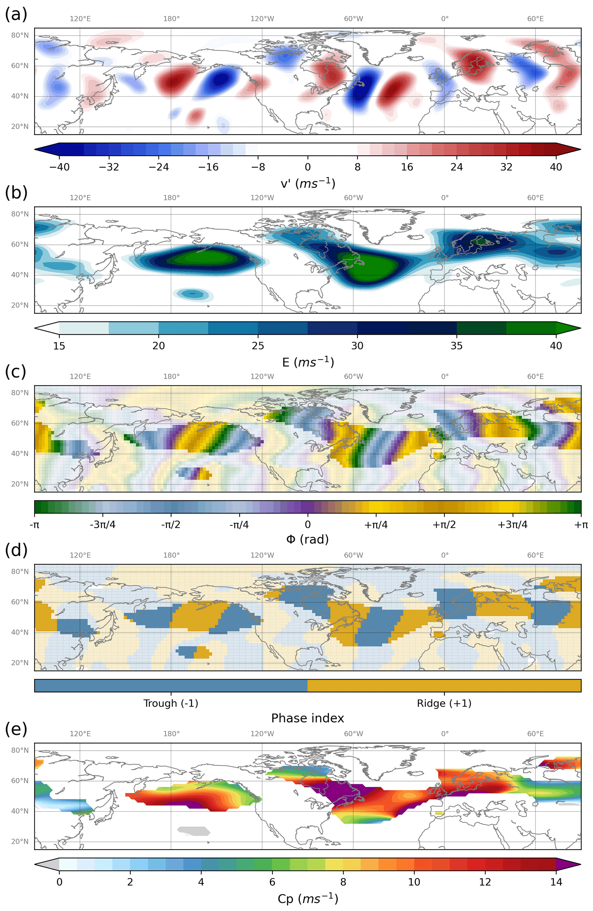
Figure 1Upper-tropospheric flow diagnostics based on the ERA5 300 hPa meridional wind anomaly (v′) field on 22 September 2018 at 00:00 UTC: (a) spatially filtered v′, (b) amplitude (E), (c) phase (Φ), (d) phase index (ridges: +1, troughs: −1), and (e) zonal phase speed (cp). Opaque colours in panels (c) and (d) indicate the areas where RWP objects are detected.
2.3 Detection and amplitude of Rossby wave packet troughs and ridges
The information about the local amplitude and phase in the v′ field is further exploited in a novel method for the detection of trough and ridge features. At first, a phase index field is constructed based on the instantaneous Φ field as follows. Phase values between 0 and π are found in the longitudinal ranges between local maxima in southerlies and northerlies (i.e. purple and green colours in Fig. 1c, respectively), which correspond to ridges in the Northern Hemisphere and troughs in the Southern Hemisphere. Conversely, phase values between −π and 0 correspond to troughs in the Northern Hemisphere and ridges in the Southern Hemisphere. Based on this distinction, grid points within ridges in both hemispheres are assigned a phase index of +1, while grid points within troughs in both hemispheres are assigned a phase index of −1. The resulting phase index field for the example of Fig. 1 is shown in panel (d).
The investigation of flow features evolving within the atmospheric continuum requires the introduction of one or more thresholds to define and spatially delimit them. In order to define trough and ridge features in this study, discernible RWP structures are identified in the flow based on a local amplitude threshold of 15 m s−1 as per FW20. Opaque colours in Fig. 1c and d indicate the grid points that satisfy this condition (i.e. E≥15 m s−1 for the given grid point and its adjacent grid points in longitude, latitude, and time) on this particular instant and thus comprise RWP objects. Troughs and ridges are herein defined as these areas within the RWP objects that have a phase index value of −1 and +1, respectively (Fig. 1d).
2.4 Diagnosis of local Rossby wave packet phase speed
When it comes to the temporal evolution of the upper-tropospheric midlatitude flow, another important property of RWPs emerges. In particular, the typically eastward motion of troughs and ridges reflects the fact that the v′ phase field varies in both space and time, thus giving rise to the concept of local RWP phase speed. In general, the phase function for a zonally propagating wave of angular wavenumber k(x,t) and angular frequency ω(x,t) is given by
where Φ0 is the phase at x=0 and t=0. The local-in-space and local-in-time zonal phase speed is thus given by
where λ denotes longitude (, with ), ϕ denotes latitude, and a denotes the Earth's radius. Given the Φ field at every latitude, longitude, and time, ω and k are computed at those grid points that comprise RWP objects (FW20). As is evident from Fig. 1e, the resulting cp field in this example is neither erratic nor uniform within the individual RWP objects; it exhibits gradual variation at synoptic scales. Overall, the example of Fig. 1 indicates that the upper-tropospheric wind field is generally characterized by transient synoptic-scale waves, with troughs and ridges forming RWPs of spatiotemporally varying amplitude and phase, the investigation of which requires local-in-space and local-in-time diagnostics.
2.5 Magnitude and monotonicity of decadal trends
The linear trends in the annual time series of various metrics associated with the RWP properties introduced above are evaluated by the Theil–Sen estimator (Sen, 1968), i.e. the median slope of lines connecting any two data points. This approach reduces the sensitivity of the trend magnitude to outliers compared to the least squares method, which is rather crucial for time series like those assessed in this study that can be characterized by pronounced interannual variability. Prior to evaluating the trend magnitude, the time series of every grid point are standardized. This allows the assessment and interpretation of the trends with respect to the local climatology (i.e. the 1979–2019 mean of a given field and season) and interannual variability (approximated by the standard deviation of a given field's seasonal mean).
Assuming that the analysed time series consist of independent random variables, the statistical significance of the detected trends over time is assessed via the non-parametric Mann–Kendall test for the null hypothesis that there is no “monotonic” trend (Gilbert, 1987; Serinaldi and Kilsby, 2016). A “monotonic” positive (negative) trend herein denotes that the variable under consideration gradually increases (decreases) with time such that the decadal trend outweighs the year-to-year variations, and thus the null hypothesis can be rejected at the given significance level. The seasonal means of consecutive years are expected – and indeed found – to be largely independent (i.e. the lag-1 autocorrelation is close to zero) for all examined fields in this study (not shown). Consequently, prewhitening the annual time series of every grid point leads to minor changes in the statistical significance patterns of the resulting trends.
3.1 Decadal variability and trends in the Rossby wave packet amplitude probability distribution over the NE Pacific and N Atlantic
To start with, the interannual and decadal variability of RWP amplitude (E) in specific regions of the Northern Hemisphere midlatitudes is explored. In doing so, the sensitivity to the chosen dataset is also assessed by employing an ensemble of three modern-era and two historical reanalyses. Although all these datasets are produced using a fixed model version and data assimilation system, the modern-era ones employ observations from a dynamic array of remote and in situ measurement techniques, while the historical ones are restricted to conventional surface observations (mainly pressure and marine wind). This stems from a difference in the purpose of these datasets. Modern-era reanalyses primarily aim at reconstructing the best possible state of the atmosphere at any given time, while historical reanalyses primarily aim to reduce the artificial low-frequency variability of meteorological variables induced by the ever-changing instrumentation.
Figure 3 shows the annual time series of DJF and JJA seasonal-mean E at 300 hPa in the NE Pacific and N Atlantic regions, while the corresponding analyses for the other four regions of Fig. 2 are included in the Supplement (Figs. S1 and S2). Locally weighted scatterplot smoothing (LOWESS) curves (Cleveland, 1979) are constructed by time series regression (using a tricube weight function) to the % nearest data points, where N is the total number of years available in each reanalysis dataset, i.e. 41 for ERA5 and JRA-55, 40 for MERRA-2, 111 for ERA-20C, and 110 for CERA-20C. These smoothed curves aim to highlight decadal variability against “noise” from interannual variability (thin solid lines in Fig. 3).
The two studied regions exhibit qualitatively different E variations in DJF (Fig. 3a, b). In particular, the NE Pacific is associated with a more pronounced interannual and decadal variability than the N Atlantic; therefore decadal trends may be harder to identify and more sensitive to the chosen time window. The NE Pacific year-to-year variability weakens in JJA, so the two regions become less distinct from each other in this season. When it comes to decadal variability, the two regions appear to experience a steady negative E trend in JJA during the past 4 decades, while the situation is less clear in DJF. Between 1920 and 1980, there is a pronounced positive E trend in the N Atlantic for both seasons and in the NE Pacific for JJA. The NE Pacific exhibits unique variability in DJF as well, as it features a distinctive double maximum between 1940 and 1980. Interestingly, a positive E trend between 1920 and 1980 is also observed in both seasons of the other four regions outlined in Fig. 2 (Figs. S1 and S2).
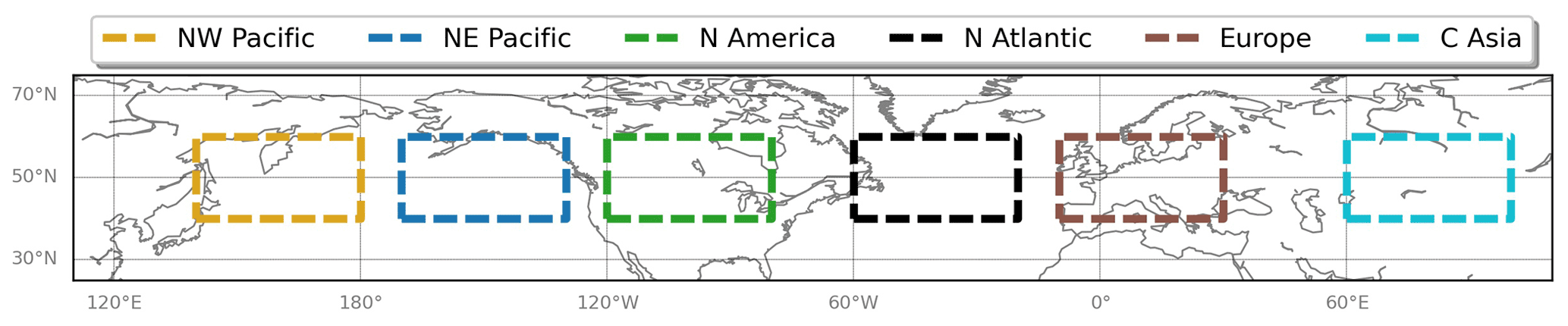
Figure 2The rectangles outline six regions in the Northern Hemisphere midlatitudes where dedicated analyses are performed in parts of this study. The six regions extend from 40 to 60∘ N in latitude and are restricted to the 140∘ E–180∘, 170–130∘ W, 120–80∘ W, 60–20∘ W, 10∘ W–30∘ E, and 60–100∘ E longitudinal ranges for the NW Pacific (yellow), NE Pacific (blue), N America (green), N Atlantic (black), Europe (brown), and central Asia (cyan), respectively.
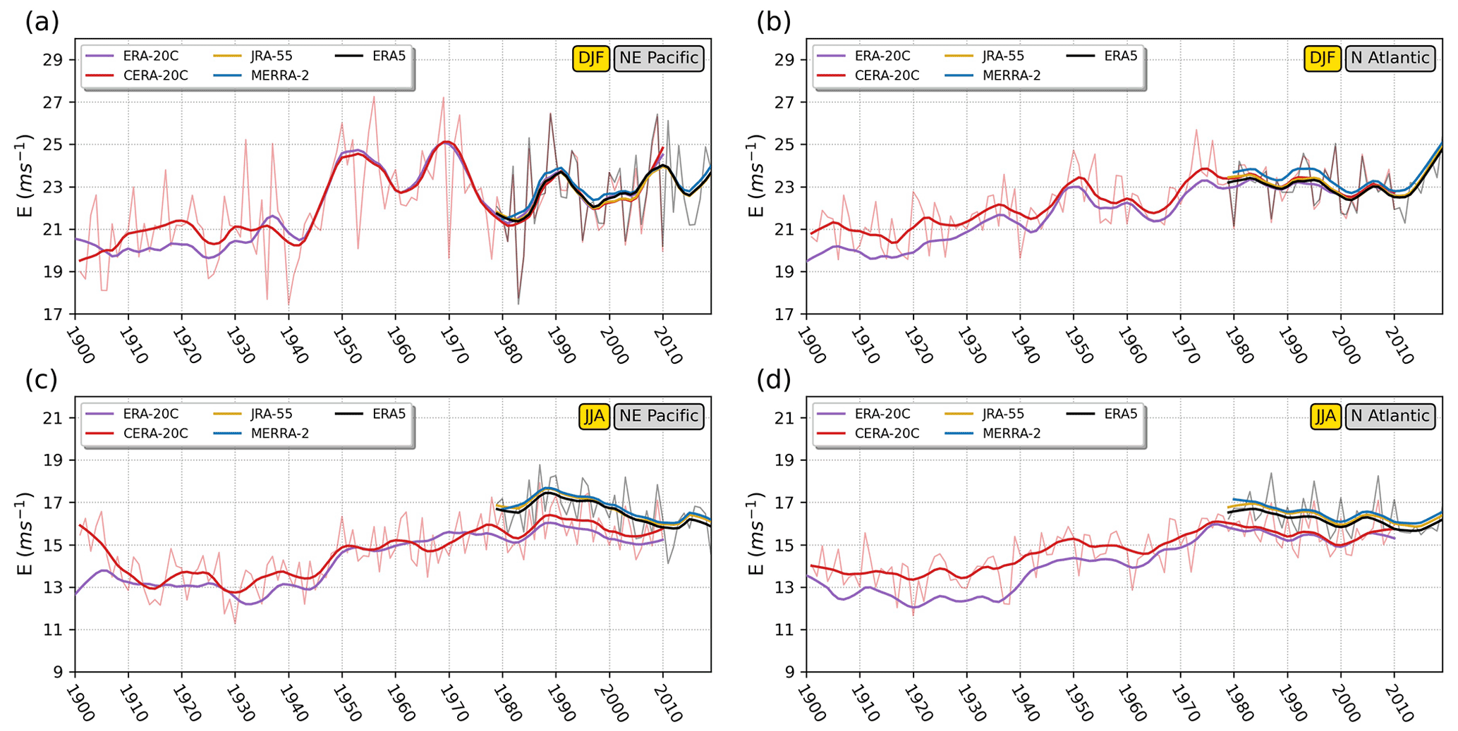
Figure 3(a) LOWESS time series of DJF-mean E at 300 hPa over NE Pacific based on the CERA-20C (red), ERA-20C (purple), JRA-55 (yellow), MERRA-2 (blue), and ERA5 (black) reanalysis. The thin red and black lines correspond to the original DJF-mean time series in CERA-20C and ERA5, respectively. (b) Same as panel (a), but for the N Atlantic region. (c, d) Same as panels (a) and (b), but for the JJA season.
Comparing the seasonal-mean E evolution in the different datasets reveals that the three modern-era reanalyses are in close agreement with each other. The magnitude of seasonal-mean E is systematically slightly higher in MERRA-2 than ERA5, while that of JRA-55 falls in between the two most of the time. During the past 4 decades, agreement between modern-era and historical reanalysis datasets is evident for DJF. Interestingly, this is not the case in JJA where the historical reanalyses appear to systematically underestimate E by about 1 m s−1 compared to the modern-era reanalyses. This suggests that the summer upper-tropospheric circulation in the evaluated historical reanalyses might not be well constrained by the available surface observations in these two storm-track regions. This problem in historical reanalyses is more pronounced in the Southern Hemisphere extratropics (not shown). There are also distinct differences between the two historical reanalyses. Although the more advanced CERA-20C provides a more realistic picture than ERA-20C (Laloyaux et al., 2018), exploring both showcases the changes in the E annual time series that can be expected in data-sparse periods when upgrading the model version and data assimilation system. A secondary factor to consider here is the spread between different CERA-20C members. This spread, however, only appears pronounced in the NE Pacific during the first 2 decades of the 20th century as indicated by Fig. S3.
In line with the apparent correlation in seasonal-mean E between all examined reanalysis datasets during the past 4 decades (Fig. 3), the analyses that follow focus on this period and are found to be insensitive to the dataset of choice. Consequently, the remainder of this study only involves the ERA5 dataset. Apart from the central tendency (represented in Fig. 3 by the seasonal mean), it is also important to investigate the decadal variability of the entire E probability distribution. Figure 4 shows the daily-mean E probability density functions (PDFs) for the NE Pacific and N Atlantic in DJF and JJA. Instead of individual years, the different PDFs correspond to rolling 5-year periods colour-coded from blue to red corresponding to 1979–1983 and 2015–2019, respectively. This is done in order to get smoother PDFs and emphasize the decadal variability. The PDF of each 5-year period is constructed based on a (non-parametric) kernel density estimation using Gaussian kernels, the bandwidth of which is selected based on Scott's rule of thumb (Scott, 1992).
A gradual shift toward higher E values is observed in the NE Pacific for DJF, which is mostly evident in the lower and near-average values of the distribution (Fig. 4a). Conversely, a uniform shift toward lower E values is observed for the narrower distribution of JJA (Fig. 4c). In the N Atlantic region, there are no equally apparent uniform shifts in the distribution as in the case of the NE Pacific. Specifically, no part of the DJF distribution appears to exhibit clearly visible shifts (Fig. 4b), whereas a decreasing occurrence in RWPs of above-average E (i.e. RWPs with E values that clearly exceed the climatological PDF maximum) is evident in JJA (Fig. 4d).
Figure 5 shows the decadal trends (based on the Theil–Sen estimator) and the corresponding 90 % confidence interval for 9 percentiles of the 5-year E probability distributions in the two regions and seasons. It illustrates the fact that all parts of the NE Pacific distribution exhibit positive trends in DJF and negative trends in JJA, with some variation between the percentiles that indicates changes in the distribution shape. As suggested by the visual inspection of Fig. 4b and d, the N Atlantic is characterized by trends of lower magnitude. Although the negative trends in JJA are nearly uniform, DJF features an increase in the lower E values and a decrease in the above-average ones such that a narrowing of the distribution arises. The generally larger confidence intervals in the percentile trends of the NE Pacific compared to those of the N Atlantic reflect the aforementioned pronounced interannual and decadal variability of the former region.
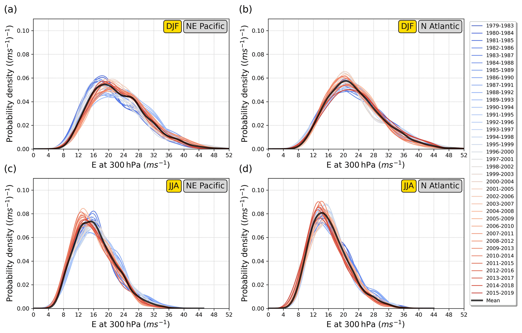
Figure 4(a) Climatological (1979–2019) PDF of the DJF daily-mean E at 300 hPa over NE Pacific based on ERA5 (black line). The coloured lines depict the corresponding PDFs of successive 5-year periods, as indicated in the legend to the right. (b) Same as panel (a), but for the N Atlantic region. (c, d) Same as panels (a) and (b), but for the JJA season.
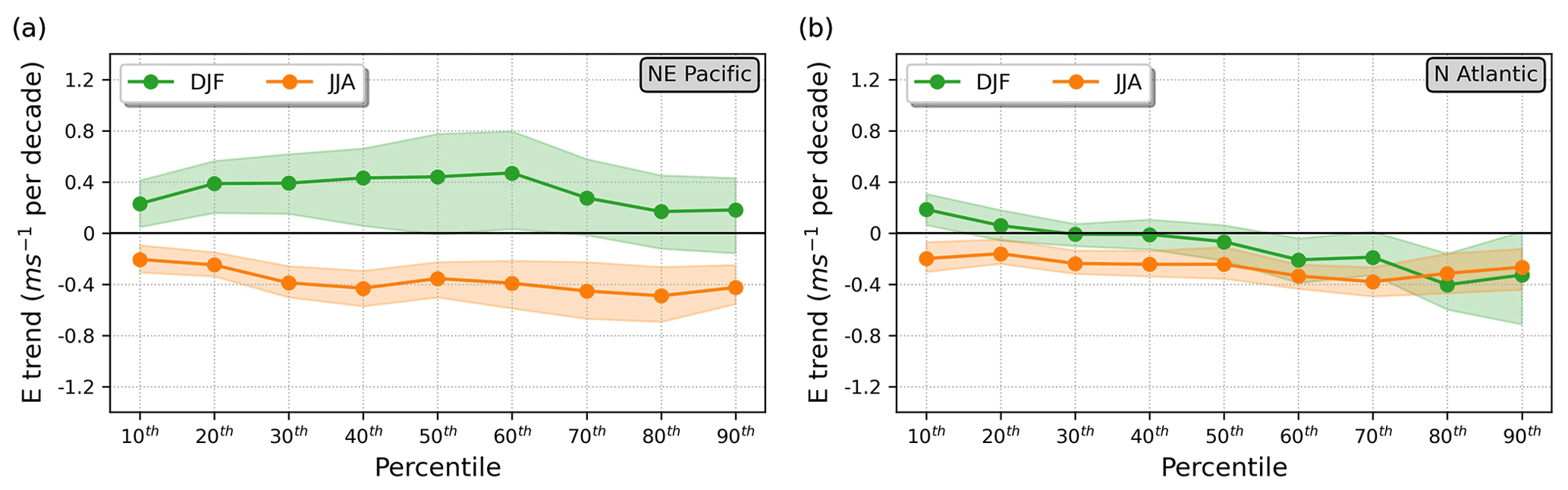
Figure 5(a) Graph of 1979–2019 linear trends (Theil–Sen estimator; connected dots) in 9 percentiles of the DJF (green) and JJA (orange) NE Pacific 5-year PDFs (Fig. 4a, c) of daily-mean E at 300 hPa in ERA5. The shading indicates the 90 % confidence interval. (b) Same as panel (a), but for the N Atlantic region.
3.2 Spatial distribution of trends in Rossby wave packet properties
Overall, Figs. 3–5 showcase the need to explore the upper-tropospheric circulation variability using diagnostics of local RWP properties for each season separately. In this subsection, the diagnostics presented in Sect. 2 are utilized to produce maps of 1979–2019 linear trends in seasonal-mean RWP amplitude (E), phase (Φ), and phase speed (cp) at 300 hPa for the Northern and Southern Hemisphere extratropics (Figs. 6–8). Given that the annual time series for each grid point are standardized, the decadal trends are given in units of standard deviations (σ) per decade (Sect. 2.5). The Mann–Kendall test assesses at each grid point the null hypothesis that the corresponding trend is not monotonic at the α=0.1 significance level. Finally, overlaid in the maps are the respective multi-year seasonal means, which are more thoroughly discussed in FW20.
3.2.1 Amplitude
Figure 6 shows the 1979–2019 trends in standardized seasonal-mean E at 300 hPa for the Northern and Southern Hemisphere extratropics, as well as the respective climatological-mean E. Evidently, several regions undergo monotonic trends in this field (indicated by red hatching), while a pronounced regional and seasonal variability – as hinted in Sect. 3.1 – thereof emerges.
The Northern Hemisphere winter season features mostly positive E trends in the midlatitudes with statistically significant values in the N Pacific, NE Atlantic, and S Asia, whereas monotonic negative E trends are found at higher latitudes including NE Canada, Greenland, and Siberia (Fig. 6a). A widespread negative E trend is evident for the summer season with several regions in the midlatitudes exhibiting statistically significant values (Fig. 6c). Opposite trends characterize large parts of the N Pacific and N Atlantic regions in MAM, with positive and negative values, respectively (Fig. 6b). Finally, negative trends emerge in areas of N America, the N Atlantic, and Eurasia in SON, but only a few parts of these regions exhibit monotonic trends (Fig. 6d).
In the Southern Hemisphere summer season (DJF), a poleward shift in the fairly zonal band of climatologically maximum E values is apparent (Fig. 6a). Namely, there is a weakening in its subtropical edge and a strengthening in its poleward edge and other areas of the Antarctic. Positive trends in middle and high latitudes span a large area in MAM (Fig. 6b), while less uniform signals emerge in JJA and SON (Fig. 6c, d).
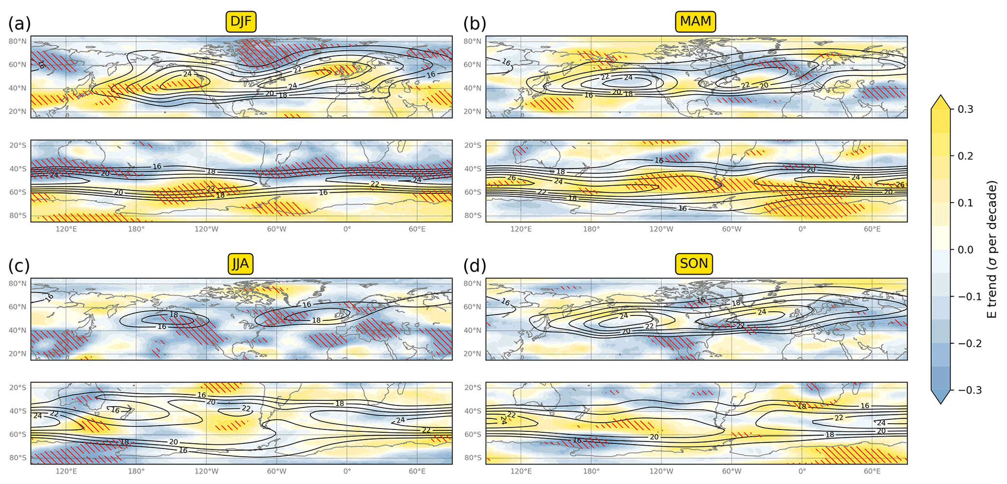
Figure 6Maps of 1979–2019 linear trends (Theil–Sen estimator; colour shading) in the standardized seasonal-mean E at 300 hPa for (a) DJF, (b) MAM, (c) JJA, and (d) SON in ERA5. Red hatching indicates areas where the trend monotonicity is statistically significant at the 0.10 significance level. Black contours correspond to the climatological-mean (1979–2019) E field of the respective season.
3.2.2 Phase
Whether a region undergoes a decadal trend in RWP amplitude or not, it is essential to examine the possibility of trends in RWP phase as well. Even in areas where E exhibits no monotonic trend, a change in the trough–ridge occurrence ratio over time may signify changes in the local weather and climate. To that end, the seasonal-mean RWP phase index is computed based on those time instances that feature an RWP object (Sect. 2.3). This metric can take any value between −1 and +1, indicating whether and by how much troughs or ridges prevail in the given location and season. It is above zero when ridges occur more often than troughs and below zero in the opposite case. For instance, a seasonal-mean phase index of +0.2 indicates that in a given grid point 60 % of the times in a season that a RWP object is present correspond to a ridge and 40 % of the times correspond to a trough.
Figure 7 shows the 1979–2019 trends in the standardized seasonal-mean RWP phase index at 300 hPa, as well as the climatological-mean phase index. The latter is based on the full phase field of v rather than the RWP v′ field such that it reflects the climatological tendency toward positive or negative phase values associated with stationary waves. The seasonal-mean RWP phase index remains undefined for seasons when no RWP object is detected, which is a common occurrence at low latitudes. When the phase index is undefined for more than 25 % of the seasons (i.e. 11 or more out of the total 41 seasons), the trend is not computed and the grid point is masked (grey shading in Fig. 7).
The analysis reveals that monotonic trends do emerge for certain regions and seasons. Statistically significant positive trends are found in DJF over the Arctic Ocean region that corresponds to the left exit of the N Atlantic jet stream and RWP track, indicating that the occurrence frequency of ridges increases relative to that of troughs (Fig. 7a). A larger part of the midlatitudes experiences statistically significant trends in MAM (Fig. 7b). Specifically, a positive trend is found over most of Europe with negative trends upstream (N Atlantic) and downstream (Western Asia). A dipole trend pattern characterizes the Arctic Ocean, probably associated with the increasing occurrence of a cross-polar wind pattern, rather than two separate processes. Finally, negative trends are found over the Sea of Japan with an equally large region of positive trends downstream over the N Pacific.
Prominent patterns emerge in JJA with statistically significant trends of alternating signs extending from N America to central Asia (Fig. 7c). Negative trends are found in eastern N America, the NE Atlantic, and central Asia, while positive trends are found in the regions in between as well as in Greenland. When it comes to SON, positive trends are found in eastern Europe and negative in central Asia (Fig. 7d). Further to the north, negative and positive trends are found to the west and east of Greenland, respectively.
Statistically significant RWP phase trends in the Southern Hemisphere are mostly found in the central and southern sides of the RWP tracks. The most prominent trend pattern emerges in JJA with a succession of positive and negative values in the 40–80∘ S latitude band (Fig. 7c). This “wave train” formation in the RWP phase trend pattern, which is also observed in the Northern Hemisphere, is not coincidental. If a process or interaction of processes leads to a gradual (i.e. acting on decadal timescales) increase in the occurrence frequency of troughs or ridges over a particular area, transient RWPs develop upstream and, primarily, downstream accordingly such that a zonally extended phase index trend pattern of alternating signs emerges.
Given that the aforementioned trends apply to the phase index of RWP objects, their interpretation should also consider trends in the RWP frequency, which generally follows the E trends (not shown). A positive RWP phase index trend may not correspond to an increase in the occurrence frequency of ridges if it coincides with a negative trend in RWP frequency. One scenario in this case is that the reduction in troughs is larger than the reduction in ridges such that the ratio of ridges over troughs increases.
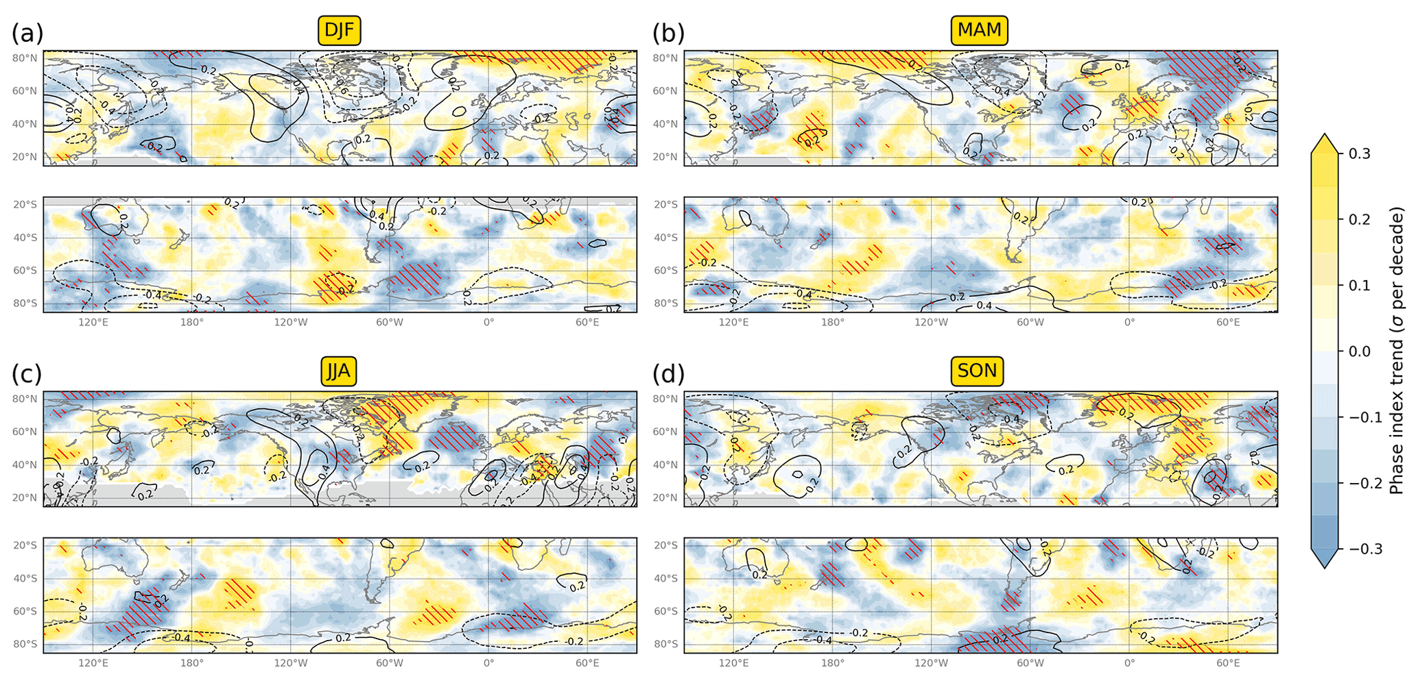
Figure 7Same as Fig. 6, but for the phase index of RWP objects at 300 hPa. Positive (negative) trends denote that the occurrence frequency of ridges increases (decreases) relative to that of troughs. The black contours correspond to the multiyear mean phase index based on the filtered v at 300 hPa (solid and dashed contours denote positive and negative values, respectively). Masked grid points are indicated by grey shading.
3.2.3 Phase speed
The possibility of decadal trends in the zonal propagation speed of RWPs (i.e. cp) is explored next. As in the case of the RWP phase index, the seasonal-mean cp is computed based on those time instances that feature an RWP object. Although no uniform slow-down or acceleration of upper-tropospheric troughs and ridges emerges in the Northern Hemisphere, certain regions in certain seasons do experience statistically significant cp trends (Fig. 8).
The most notable pattern of monotonic trends in the Northern Hemisphere occurs in MAM (Fig. 8b). The cp trend in the N Pacific is generally negative, with statistically significant values over the Philippine Sea and East China Sea, which are regions that also experience monotonic positive E trends (Fig. 6b). Monotonic negative trends also characterize Greenland and the Arctic Ocean region to the north of Europe. In contrast, the rest of the midlatitudes feature positive cp trends, with statistically significant values over most of Europe and parts of the N Atlantic and western Russia. No large-scale pattern of statistically significant trends emerges in the other seasons, except for the negative values in Siberia in DJF and the N Atlantic in JJA (Fig. 8a, c).
In contrast to the Northern Hemisphere, the Southern Hemisphere extratropics exhibit a widespread tendency toward higher cp values. Moreover, statistically significant positive trends cover large parts of the S Atlantic Ocean in DJF and MAM, the Indian Ocean in DJF, and the S Pacific Ocean in MAM and JJA. Although exploring the relation of the aforementioned trends with trends of other circulation properties is beyond the scope of this study, the corresponding trends in ERA5 zonal wind (u) at 300 hPa are provided in the Supplement for reference (Fig. S5). Finally, when expressing cp in degrees longitude per unit time (i.e. angular phase speed), minor qualitative changes occur in the instantaneous cp field of Fig. 1e, but there is no effect in the results of Fig. 8.
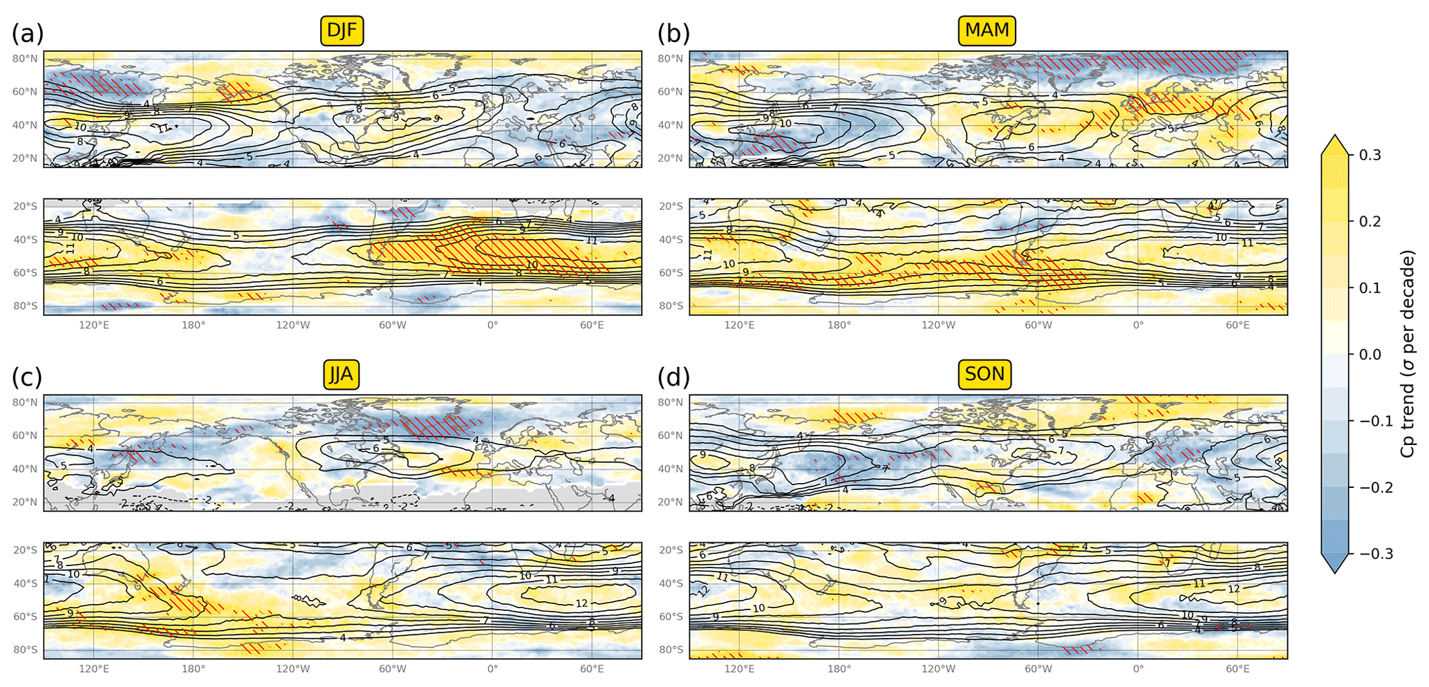
Figure 8Same as Fig. 6, but for cp at 300 hPa (solid and dashed black contours denote positive and negative climatological-mean values, respectively). As with the RWP phase index, grid points where the cp is undefined for more than 25 % of the seasons are masked (grey shading).
3.3 Trends in the Rossby wave packet amplitude and phase speed joint distribution
As indicated in Sect. 3.1, seasonal probability distributions of local RWP properties may exhibit uniform shifts and/or changes in their shape. Therefore, the aforementioned seasonal-mean trend maps are not necessarily indicative of changes in e.g. the distribution tails of the associated fields. To that end, this subsection explores the 1979–2019 decadal trends in the entire E and cp seasonal distributions for the six regions outlined in Fig. 2. Moreover, the distributions of these two properties are not investigated in isolation but jointly. This allows the inspection of possible shifts in the bivariate probability distribution function of daily-mean E and cp, hereafter denoted as , toward a certain regime. For example, it is worth knowing whether the negative E trend over a region concerns the fast wave packets, the quasi-stationary ones, or much of the cp domain. Similarly, one can focus on a specific E regime, e.g. large-amplitude RWPs, and assess the associated cp trend.
In contrast to the analysis of Fig. 4, averaging the daily-mean E and cp over a region only accounts for grid points that are occupied by RWP objects and cp is available (i.e. where E≥15 m s−1; see Sect. 2.3). Furthermore, days when an RWP object covers less than 10 % of the total region area are omitted from the E and cp time series. Based on the resulting time series, Fig. 9 shows the climatological-mean and decadal trend of the daily-mean E and cp bivariate PDF () over the aforementioned regions in the four seasons. The underlying PDFs of the entire data sample (i.e. climatological probability distribution) and the data of each season separately are derived from two-dimensional Gaussian kernel density estimations with bandwidths based on Scott's rule of thumb. The resulting two-dimensional PDFs reflect the density of the data points in the E–cp domain and have units of (m s−1)−2 (probability per unit of space). The probability density annual time series for each point in the E–cp domain is then standardized, and its decadal trend magnitude and monotonicity are evaluated as described in Sect. 2.5.
The distribution shifts emerging in Fig. 9 reflect, to some extent, the individual decadal trends of seasonal-mean E and cp shown in Figs. 6 and 8. Hereafter, apparent trend patterns in that cannot be inferred from the seasonal-mean trends of the individual fields are highlighted. Starting with DJF, the observed positive E trend over the two N Pacific regions (Fig. 6a) is associated with an increase in RWPs of high E and above-average cp (Fig. 9a, b). The positive E trend over Europe is associated with an increase in high-E average-cp RWPs and a decrease in RWPs of low E and high or low cp (Fig. 9e). Finally, the negative cp trend in C Asia (Fig. 8a) involves RWPs of any E, although the changes are generally not statistically significant (Fig. 9f).
The MAM cp trends in the NE Pacific and N America (negative and positive, respectively; Fig. 8b) primarily involve the cp distribution of RWPs with near-average E. In addition, the positive cp trend over Europe is associated with a shift from high-E, low-cp RWPs toward high-cp RWPs of weaker amplitude (Fig. 9k). Finally, the positive cp trend in C Asia is instead primarily associated with an increase in low-E, high-cp RWPs (Fig. 9l).
In JJA, the NW Pacific region experiences an increase in RWPs of below-average E and cp RWPs with a decreasing occurrence of RWPs of all other regimes (Fig. 9m). On the other hand, the NE Pacific experiences a shift from RWPs with high E and low or average cp to low-E, low-cp RWPs (Fig. 9n). No change is observed for N America, while the E reduction over N Atlantic and Eurasia appears to favour RWPs of above-average cp, which is a shift that is more prominent over Europe (Fig. 9o–r).
Fewer statistically significant changes in occur in SON compared to the other seasons (Fig. 9s–x). RWPs of low cp and above-average E over NE Pacific occur more frequently at the expense of low-E, high-cp RWPs. Despite the generally negative trends in both seasonal-mean E and cp over Eurasia (Figs. 6d and 8d), Europe exhibits a shift toward RWPs of lower cp, whereas C Asia exhibits a reduction in high-cp RWPs and an increase in the average-cp ones (i.e. a narrowing of the cp distribution for most E regimes).
Another key aspect emerging from the 24 investigated probability distributions is that there is no consistent underlying relation between the E and cp trends; that is, there is no covariance between the two properties at decadal timescales. When considering all regions, a gradual shift toward higher or lower RWP amplitudes is not necessarily associated with a shift toward lower or higher RWP phase speeds. For example, while MAM in Europe (Fig. 9k), JJA in the NE Pacific (Fig. 9n), and JJA in Europe (Fig. 9q) are all characterized by negative E trends, there is a clear positive cp trend in the first case, a slightly negative cp trend in the second case, and no apparent cp trend in the third case. As is also indicated by the climatological-mean (black contours in Fig. 9), there is no clear relationship between the fields of these two RWP object properties. Days with high E over an area are not necessarily associated with low cp, while days with low E are not necessarily associated with high cp (see also Sect. 8 in the Supplement of FW20). The reason for this and the absence of covariance in their trends is that these fields do not just depend on each other, but they are influenced by other factors as well.
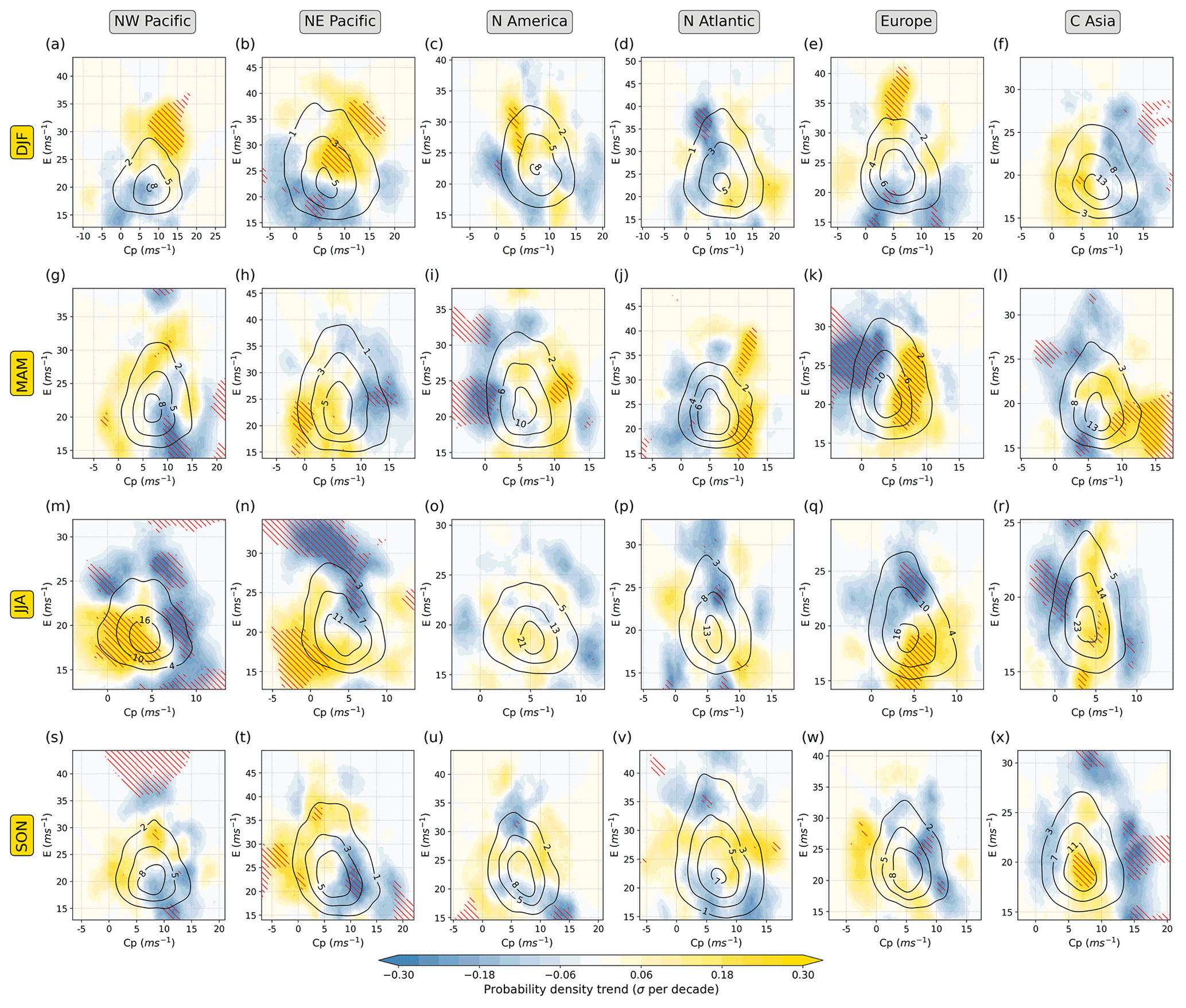
Figure 9(a–f) Climatological (1979–2019) bivariate PDF of the DJF daily-mean E and cp at 300 hPa (10−3 (m s−1)−2; black contours) over (a) the NW Pacific, (b) the NE Pacific, (c) N America, (d) the N Atlantic, (e) Europe, and (f) central Asia in ERA5. Colour shading corresponds to the 1979–2019 linear trend (Theil–Sen estimator) in the seasonal probability density of daily-mean E and cp. Red hatching indicates areas where the trend monotonicity is statistically significant at the 0.10 significance level. Panels (g–l), (m–r), and (s–x) are the same as panels (a–f), but for MAM, JJA, and SON, respectively.
3.4 Temporal variation of trends in mean and extreme RWP properties
As shown in Sect. 3.1, the NE Pacific experiences pronounced decadal variability in the seasonal-mean E field in DJF (Fig. 3). This suggests that, when considering shorter periods within 1979–2019, the respective trends in RWP properties may exhibit significant temporal variation in some regions and seasons. The objectives of this subsection are, firstly, to underline and illustrate this aspect and, secondly, to report on the associated variability in the occurrence frequency of RWP amplitude and phase speed extremes.
Figure 10 provides an example of pronounced temporal variation in seasonal-mean E and cp trends by separating the Northern Hemisphere DJF analysis into the two equally long periods of 1979–1999 and 1999–2019. Evidently, many areas are characterized by E and cp trends of different signs in these two periods. A big part of the 15–40∘ N latitude band – including the N Pacific, the Mediterranean, and Asia – shifts from weakly negative (during 1979–1999) to positive and often monotonic (during 1999–2019) E trends. Furthermore, areas to the north of 60∘ N experience an apparent change from monotonic negative to weak E trends. Between 40 and 60∘ N, the E trends remain mostly positive throughout the 41-year period. When it comes to cp, a positive trend during 1979–1999 characterizes much of the Northern Hemisphere extratropics, albeit with infrequent monotonicity. In contrast, monotonic negative trends are found over parts of Asia, the N Pacific, and N America during the 1999–2019 period. In particular, an unusual period of five consecutive winters between 1998 and 2002 with relatively high cp values over the NE Pacific (Fig. S4) appears crucial for the noticeable trend change in this area and suggests that the scarcity of monotonic cp trends in the 1979–2019 period (Fig. 8a) is caused by variability at both interannual and longer timescales.
The last part of this study focuses on the tails of the E and cp seasonal distributions exclusively and assesses trends in the occurrence frequency of high-E and low-cp extremes. This is motivated by the documented role of these two RWP properties in hot and cold extremes throughout the year (Sect. 1). High-E extremes are defined as days when the daily-mean RWP amplitude exceeds the climatological 90th percentile of the given grid point and year day. Similarly, low-cp extremes are defined as days when the daily-mean RWP phase speed does not exceed the climatological 10th percentile. The potentially more alarming situations when RWPs are both large-amplitude and quasi-stationary constitute a subset of the E–cp domain that merits particular attention. To that end, compound extremes are defined as days when the daily-mean RWP amplitude exceeds the climatological 70th percentile and the daily-mean RWP phase speed does not exceed the climatological 30th percentile. The computation of the aforementioned climatological percentiles for each day of the year is described in Appendix A.
The Northern Hemisphere DJF trends in high-E, low-cp, and compound extremes during the 1979–1999 and 1999–2019 periods are shown in Fig. 11, while the 1979–2019 global trends are provided in the Supplement for reference (Figs. S6–S8). The count of extremes is regarded as 0 (i.e. it is not undefined) for seasons with no detected RWP object, which is typical for low-latitude grid points. Overall, the analysis demonstrates that the aforementioned temporal variation of trends in seasonal-mean E and cp is also reflected in the justifiably spottier and less statistically significant trend patterns of their extremes. The 1979–1999 positive high-E extreme trends between 40 and 60∘ N and negative trends to the north and south of this band are succeeded by generally positive trends during 1999–2019; more prominently over the N Pacific, China, northwestern N America, and the Mediterranean. In the case of low-cp and compound extremes, a large part of the N Pacific and N America regions experiences weak to no trends in 1979–1999, but shifts to positive and often monotonic trends in 1999–2019. Given that midlatitude grid points experience on average around five high-E, five low-cp, and four compound extremes per winter3, monotonic positive trends of 0.2 extremes per year may be hardly perceptible to society, albeit rather substantial in the course of 20 years.
Since this subsection aims to underline and illustrate the possibility for temporally varying trends in shorter periods within 1979–2019, restricting the analysis to the Northern Hemisphere DJF season serves the purpose. Nevertheless, the respective analyses of Fig. 11 for the other seasons are provided in the Supplement (Figs. S9–S11). A notable aspect is that SON shows similar behaviour as DJF over parts of the N Pacific in terms of the temporal trend variation in the three types of extremes. Smaller patterns of statistically significant trends emerge in MAM, with a decrease in high-E extremes over parts of Asia during 1979–1999 and N America during 1999–2019, as well as an increase during 1999–2019 in high-E and low-cp extremes over parts of the N Atlantic and N Europe, respectively. No apparent trends emerge in JJA, except from an increase in low-cp extremes over parts of the N Pacific and N America during 1979–1999. In general, the results of this subsection demonstrate that temporally varying trends emerge within 1979–2019 in the E and cp seasonal distributions of some regions and seasons, and this reflects on the occurrence of large-amplitude and/or quasi-stationary RWPs.
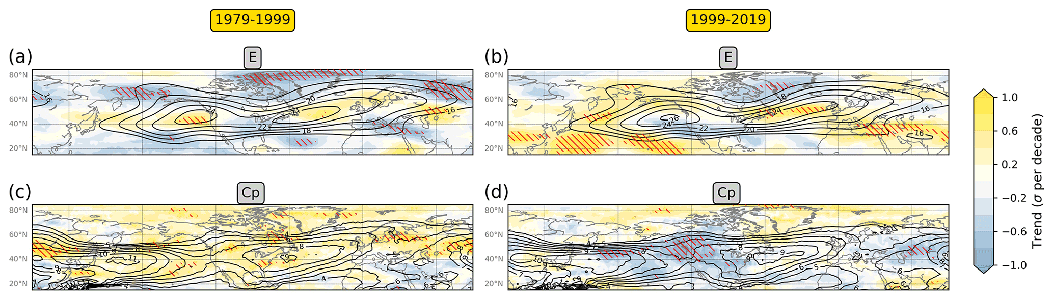
Figure 10Maps of 1979–1999 linear trends (Theil–Sen estimator; colour shading) in the standardized seasonal-mean (a) E and (c) cp at 300 hPa for DJF in ERA5. (b, d) Same as panels (a) and (c), but for 1999–2019. Red hatching indicates areas where the trend monotonicity is statistically significant at the 0.10 significance level. Black contours correspond to the multiyear mean fields of the respective period. Masked grid points are indicated by grey shading.
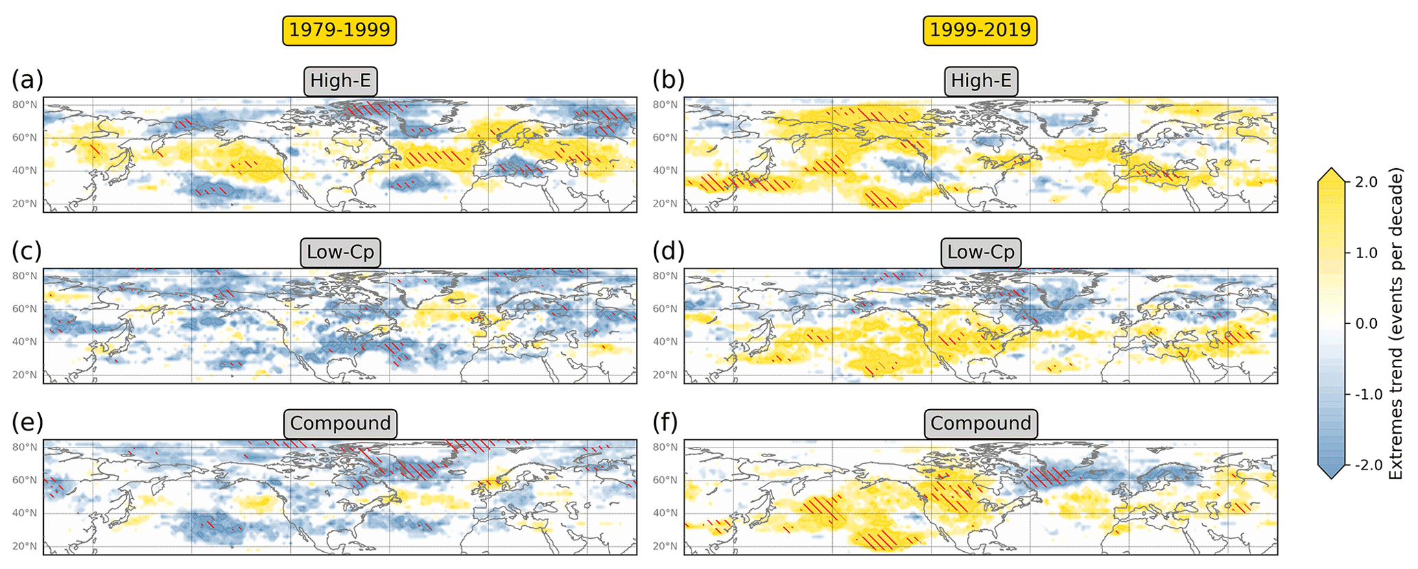
Figure 11Maps of 1979–1999 linear trends (Theil–Sen estimator; colour shading) in the number of (a) high-E extremes, (c) low-cp extremes, and (e) compound high-E/low-cp extremes at 300 hPa for DJF in ERA5. (b, d, f) Same as panels (a), (c), (e), but for 1999–2019. Red hatching indicates areas where the trend monotonicity is statistically significant at the 0.10 significance level.
This study assessed the decadal variability of the extratropical upper-tropospheric circulation by utilizing reanalysis data and diagnostics of local-in-space and local-in-time RWP amplitude (E), phase (Φ), and phase speed (cp) at 300 hPa. The main outcomes are summarized hereafter.
-
The analysis of area-averaged seasonal-mean E time series during the 1900–2019 DJF and JJA seasons showed that the NE Pacific exhibits a more pronounced interannual and decadal variability than the N Atlantic, while both regions feature less interannual variability in JJA. The examined modern-era (ERA5, JRA-55, and MERRA-2) and historical (ERA-20C and CERA-20C) reanalysis datasets were found to be in close agreement with each other regarding the seasonal-mean E value in DJF, but less so in JJA where the historical ones systematically underestimate E. Focusing on the 1979–2019 period in ERA5, the decadal evolution of the daily-mean E probability distribution indicated seasonally and regionally varying trends in its mean and shape. Specifically, all parts of the NE Pacific E distribution exhibit a positive trend in DJF and negative trend in JJA, while the N Atlantic E distribution undergoes a narrowing in DJF and a shift toward smaller values in JJA.
-
Trends in the seasonal-mean RWP properties in the entire Northern and Southern Hemisphere extratropics were then assessed and some notable patterns of statistically significant values are highlighted here. A substantial part of the N Pacific, the NE Atlantic, and S Asia undergoes positive E trends in DJF, whereas an E decrease is found in areas at higher latitudes in DJF and much of the Northern Hemisphere extratropics in JJA. The Southern Hemisphere extratropics are characterized by a poleward shift in the band of climatologically maximum E values in DJF and widespread positive E trends in MAM. Zonally extended trend patterns of alternating signs emerge in the trough–ridge occurrence ratio for MAM in the Northern Hemisphere and JJA in both hemispheres. When it comes to cp, MAM features positive trends over parts of the N Atlantic and most of Europe, as well as negative trends to the north of these regions and much of the N Pacific. Furthermore, high-latitude areas of the N Atlantic experience negative cp trends in JJA, while positive trends cover large parts of the Southern Hemisphere in DJF and MAM.
-
An assessment of changes in the bivariate probability distribution of daily-mean E and cp demonstrated that the aforementioned Northern Hemisphere trends are associated with varying shifts in the E–cp domain between seasons and regions, thus suggesting the absence of covariance between E and cp at decadal timescales.
-
As illustrated for the Northern Hemisphere E and cp fields in DJF, interannual and/or decadal variability prevails in many areas that do not exhibit monotonic trends in the 1979–2019 period. Associated with that, it was found that sizable portions of the N Pacific and N America regions experience positive trends in the occurrence frequency of large-amplitude and/or quasi-stationary RWPs in DJF during 1999–2019.
Overall, these results underscore that substantial seasonal and regional variations characterize the past decadal variability in RWP amplitude, phase, and phase speed, while monotonic trends emerge in the probability distributions of these fields for specific areas, seasons, and time periods.
The presented analyses do not change qualitatively when performed at the 250 or 350 hPa levels instead of 300 hPa. Setting the RWP object identification threshold to 10 or 20 m s−1 leads to no substantial change in the seasonal-mean phase and phase speed trends (Figs. 7 and 8). In addition, as indicated by Fig. 3, the results remain largely unchanged when employing the JRA-55 or MERRA-2 datasets instead of ERA5. One exception here is that JRA-55 features widespread monotonic positive E trends in the Southern Hemisphere high latitudes (i.e. to the south of 60∘ S) in all seasons between 1979 and 2019, thus differing substantially from ERA5 (Fig. 6) and MERRA-2. The spatial variation in the E and cp trends that could be unveiled through the use of local-in-space diagnostics (Figs. 6 and 8) implies that the analyses of Sect. 3.1 and 3.3 are sensitive to the size and location of the rectangles for some regions and seasons (Fig. 2). Also accounting for the pronounced temporal variation in the trends of some regions (Sect. 3.4), it becomes evident that trends in such properties of the upper-tropospheric flow should be interpreted with caution when focusing on specific areas and/or short time periods. Information regarding the advantages and limitations of the employed RWP diagnostics is provided in FW20. It is worth noting that these diagnostics account for flow configurations that locally resemble almost plane waves of discernible zonal wavenumber and angular frequency. This means that they are not supposed to accurately capture wave-breaking, where the emergence of filamentary and cutoff structures implies the wave decay. Since both E and cp typically decrease in these situations, the presented trends may also encompass an effect from possible trends in the wave breaking occurrence.
Owing to differences in the employed diagnostic methods and incompatibilities in the time periods and areas under consideration, a direct comparison with previous studies mentioned in Sect. 1 is barely possible. However, the reported widespread E decrease in the Northern Hemisphere JJA season (Fig. 6c) is consistent with the Coumou et al. (2015) spectral analysis of the midlatitude 500 hPa meridional wind field. In addition, although positive and negative cp trends do emerge in some areas of the Northern Hemisphere in DJF and JJA, there is no overall consistent trend in the midlatitudes, in agreement with the results of Riboldi et al. (2020).
The reported trends in RWP properties are most likely influenced by both externally and internally generated variability (Shepherd, 2014; Deser et al., 2016), though weighing the individual contributions was beyond the scope of this study. Moreover, the observed trend patterns in this study suggest that any future trends in the extratropical upper-tropospheric circulation – especially in the Northern Hemisphere – will not necessarily be zonally symmetric or meridionally homogeneous (see also Simpson et al., 2014). In an effort to expose such inhomogeneities, the employed methodology allowed the assessment of decadal variability and trends in RWPs without obscuring their highly dynamic and spatially varying properties at weather timescales. This approach facilitates the investigation and interpretation of circulation-related mechanisms that influence regional climate and future projections of weather extremes.
Questions regarding the causes and implications of statistically significant trends reported in this study naturally arise. Why has the RWP amplitude been decreasing during 1979–2019 in much of the Northern Hemisphere extratropics in summer and how much has this contained, if at all, the past increase in warm extremes? What drives the positive RWP amplitude trends during 1920–1980 in the Northern Hemisphere midlatitudes, as observed in the tested historical reanalyses? Do trends in the phase of Rossby waves (e.g. the negative trend over the NE Atlantic in JJA) have an effect on temperature trends and the occurrence of weather extremes? What is the relation of trends in RWP properties to trends in zonal wind? Such investigations require and deserve dedicated studies.
The climatological annual cycles of the RWP amplitude and phase speed percentiles for a specific grid point and day of the year are computed as follows. Due to the small number of available years, each day of the year is represented by a probability distribution that comprises all daily-mean E or cp values in the 21 d windows centred around it in every year. This results in a sample size of up to 861 data points (21 values from each of the 41 available years). Days when an RWP object is not identified in the given grid point are not included in the distribution, so its size decreases accordingly. The climatological nth percentile is computed based on this distribution, which means that in the case of E the minimum value in the distribution is 15 m s−1. The climatological annual cycle of the nth percentile is then constructed by repeating the above for every day of the year and it is subsequently smoothed by restriction to frequencies 0–4 yr−1 (as in the case of the climatological mean; Sect. 2.2).
The reanalysis data used in this study are freely available online (Sect. 2.1) and can be accessed as described in Sect. 9 of the Supplement. Processed data and code employed in the presented analyses can be provided by the author upon request.
The supplement related to this article is available online at: https://doi.org/10.5194/wcd-3-1381-2022-supplement.
The author has declared that there are no competing interests.
Publisher’s note: Copernicus Publications remains neutral with regard to jurisdictional claims in published maps and institutional affiliations.
The author acknowledges ECMWF, NASA, and JMA for providing free access to the reanalysis data and Johannes Gutenberg University Mainz for granting computing time on the supercomputer Mogon II (https://hpc.uni-mainz.de/, last access: 23 October 2022). Finally, the author is grateful to two anonymous reviewers as well as Volkmar Wirth and Franziska Teubler for constructive feedback on earlier versions of the paper.
This research has been supported by the Deutsche Forschungsgemeinschaft (DFG; grant no. 445572993).
This paper was edited by Irina Rudeva and reviewed by two anonymous referees.
Ali, S. M., Martius, O., and Röthlisberger, M.: Recurrent Rossby Wave Packets Modulate the Persistence of Dry and Wet Spells Across the Globe, Geophys. Res. Lett., 48, e2020GL091452, https://doi.org/10.1029/2020GL091452, 2021. a
Blackport, R. and Screen, J. A.: Insignificant effect of Arctic amplification on the amplitude of midlatitude atmospheric waves, Science Advances, 6, eaay2880, https://doi.org/10.1126/sciadv.aay2880, 2020. a
Branstator, G. and Teng, H.: Tropospheric Waveguide Teleconnections and Their Seasonality, J. Atmos. Sci., 74, 1513–1532, https://doi.org/10.1175/JAS-D-16-0305.1, 2017. a
Cleveland, W. S.: Robust locally weighted regression and smoothing scatterplots, J. Am. Stat. Assoc., 74, 829–836, https://doi.org/10.1080/01621459.1979.10481038, 1979. a
Cohen, L.: Time-frequency analysis, Prentice Hall PTR, ISBN-10: 0-13-594532-1, ISBN-13: 978-0-13-594532-2, 1995. a
Coumou, D., Lehmann, J., and Beckmann, J.: The weakening summer circulation in the Northern Hemisphere mid-latitudes, Science, 348, 324–327, https://doi.org/10.1126/science.1261768, 2015. a, b
Deser, C., Terray, L., and Phillips, A. S.: Forced and internal components of winter air temperature trends over North America during the past 50 years: Mechanisms and implications, J. Climate, 29, 2237–2258, https://doi.org/10.1175/JCLI-D-15-0304.1, 2016. a
Di Capua, G. and Coumou, D.: Changes in meandering of the Northern Hemisphere circulation, Environ. Res. Lett., 11, 094028, https://doi.org/10.1088/1748-9326/11/9/094028, 2016. a
Feldstein, S. B. and Dayan, U.: Circumglobal teleconnections and wave packets associated with Israeli winter precipitation, Q. J. Roy. Meteor. Soc., 134, 455–467, https://doi.org/10.1002/qj.225, 2008. a
Fragkoulidis, G. and Wirth, V.: Local rossby wave packet amplitude, phase speed, and group velocity: Seasonal variability and their role in temperature extremes, J. Climate, 33, 8767–8787, https://doi.org/10.1175/JCLI-D-19-0377.1, 2020. a, b
Fragkoulidis, G., Wirth, V., Bossmann, P., and Fink, A. H.: Linking Northern Hemisphere temperature extremes to Rossby wave packets, Q. J. Roy. Meteor. Soc., 144, 553–566, https://doi.org/10.1002/qj.3228, 2018. a
Gabor, D.: Theory of communication. Part 1: The analysis of information, Journal of the Institution of Electrical Engineers – Part III: Radio and Communication Engineering, 93, 429–441, https://doi.org/10.1049/ji-3-2.1946.0074, 1946. a
Gelaro, R., McCarty, W., Suárez, M. J., Todling, R., Molod, A., Takacs, L., Randles, C. A., Darmenov, A., Bosilovich, M. G., Reichle, R., Wargan, K., Coy, L., Cullather, R., Draper, C., Akella, S., Buchard, V., Conaty, A., da Silva, A. M., Gu, W., Kim, G. K., Koster, R., Lucchesi, R., Merkova, D., Nielsen, J. E., Partyka, G., Pawson, S., Putman, W., Rienecker, M., Schubert, S. D., Sienkiewicz, M., and Zhao, B.: The modern-era retrospective analysis for research and applications, version 2 (MERRA-2), J. Climate, 30, 5419–5454, https://doi.org/10.1175/JCLI-D-16-0758.1, 2017. a
Gilbert, R. O.: Statistical Methods for Environmental Pollution Monitoring, John Wiley & Sons, ISBN: 978-0-471-28878-7, 1987. a
Grazzini, F., Fragkoulidis, G., Teubler, F., Wirth, V., and Craig, G. C.: Extreme precipitation events over northern Italy. Part II: Dynamical precursors, Q. J. Roy. Meteor. Soc., 147, 1237–1257, https://doi.org/10.1002/qj.3969, 2021. a
Harnik, N., Messori, G., Caballero, R., and Feldstein, S. B.: The Circumglobal North American wave pattern and its relation to cold events in eastern North America, Geophys. Res. Lett., 43, 11015–11023, https://doi.org/10.1002/2016GL070760, 2016. a
Harris, F. J.: On the use of windows for harmonic analysis with the discrete Fourier transform, Pr. Inst. Electr. Elect., 66, 51–83, https://doi.org/10.1109/PROC.1978.10837, 1978. a
Hersbach, H., Bell, B., Berrisford, P., Hirahara, S., Horányi, A., Muñoz-Sabater, J., Nicolas, J., Peubey, C., Radu, R., Schepers, D., Simmons, A., Soci, C., Abdalla, S., Abellan, X., Balsamo, G., Bechtold, P., Biavati, G., Bidlot, J., Bonavita, M., De Chiara, G., Dahlgren, P., Dee, D., Diamantakis, M., Dragani, R., Flemming, J., Forbes, R., Fuentes, M., Geer, A., Haimberger, L., Healy, S., Hogan, R. J., Hólm, E., Janisková, M., Keeley, S., Laloyaux, P., Lopez, P., Lupu, C., Radnoti, G., de Rosnay, P., Rozum, I., Vamborg, F., Villaume, S., and Thépaut, J. N.: The ERA5 global reanalysis, Q. J. Roy. Meteorol. Soc., 146, 1999–2049, https://doi.org/10.1002/qj.3803, 2020. a
Hoskins, B. J. and Hodges, K. I.: The annual cycle of Northern Hemisphere storm tracks. Part I: Seasons, J. Climate, 32, 1743–1760, https://doi.org/10.1175/JCLI-D-17-0870.1, 2019. a
Huang, C. S. and Nakamura, N.: Local Finite-Amplitude Wave Activity as a Diagnostic of Anomalous Weather Events, J. Atmos. Sci., 73, 211–229, https://doi.org/10.1175/JAS-D-15-0194.1, 2016. a
Karami, K.: Upper tropospheric Rossby wave packets: long-term trends and variability, Theor. Appl. Climatol., 138, 527–540, https://doi.org/10.1007/s00704-019-02845-5, 2019. a
Kobayashi, S., Ota, Y., Harada, Y., Ebita, A., Moriya, M., Onoda, H., Onogi, K., Kamahori, H., Kobayashi, C., Endo, H., Miyaoka, K., and Kiyotoshi, T.: The JRA-55 reanalysis: General specifications and basic characteristics, J. Meteorol. Soc. Jpn., 93, 5–48, https://doi.org/10.2151/jmsj.2015-001, 2015. a
Laloyaux, P., de Boisseson, E., Balmaseda, M., Bidlot, J. R., Broennimann, S., Buizza, R., Dalhgren, P., Dee, D., Haimberger, L., Hersbach, H., Kosaka, Y., Martin, M., Poli, P., Rayner, N., Rustemeier, E., and Schepers, D.: CERA-20C: A Coupled Reanalysis of the Twentieth Century, J. Adv. Model. Earth Sy., 10, 1172–1195, https://doi.org/10.1029/2018MS001273, 2018. a, b
Madonna, E., Li, C., Grams, C. M., and Woollings, T.: The link between eddy-driven jet variability and weather regimes in the North Atlantic-European sector, Q. J. Roy. Meteor. Soc., 143, 2960–2972, https://doi.org/10.1002/qj.3155, 2017. a
O'Brien, L. and Reeder, M. J.: Southern Hemisphere summertime Rossby waves and weather in the Australian region, Q. J. Roy. Meteor. Soc., 143, 2374–2388, https://doi.org/10.1002/qj.3090, 2017. a
Poli, P., Hersbach, H., Dee, D. P., Berrisford, P., Simmons, A. J., Vitart, F., Laloyaux, P., Tan, D. G., Peubey, C., Thépaut, J. N., Trémolet, Y., Hólm, E. V., Bonavita, M., Isaksen, L., and Fisher, M.: ERA-20C: An atmospheric reanalysis of the twentieth century, J. Climate, 29, 4083–4097, https://doi.org/10.1175/JCLI-D-15-0556.1, 2016. a
Riboldi, J., Lott, F., D'Andrea, F., and Rivière, G.: On the Linkage Between Rossby Wave Phase Speed, Atmospheric Blocking, and Arctic Amplification, Geophys. Res. Lett., 47, e2020GL087796, https://doi.org/10.1029/2020GL087796, 2020. a, b
Röthlisberger, M., Frossard, L., Bosart, L. F., Keyser, D., and Martius, O.: Recurrent synoptic-scale Rossby wave patterns and their effect on the persistence of cold and hot spells, J. Climate, 32, 3207–3226, https://doi.org/10.1175/JCLI-D-18-0664.1, 2019. a
Scott, D. W.: Multivariate Density Estimation, Wiley Series in Probability and Statistics, Wiley, https://doi.org/10.1002/9780470316849, 1992. a
Sen, P. K.: Estimates of the Regression Coefficient Based on Kendall's Tau, J. Am. Stat. Assoc., 63, 1379–1389, https://doi.org/10.1080/01621459.1968.10480934, 1968. a
Serinaldi, F. and Kilsby, C. G.: The importance of prewhitening in change point analysis under persistence, Stoch. Env. Res. Risk A., 30, 763–777, https://doi.org/10.1007/s00477-015-1041-5, 2016. a
Shepherd, T. G.: Atmospheric circulation as a source of uncertainty in climate change projections, Nat. Geosci., 7, 703–708, https://doi.org/10.1038/ngeo2253, 2014. a, b
Simmons, A., Wallace, J., and Branstator, G.: Barotropic wave propagation and instability, and atmospheric teleconnection patterns, J. Atmos. Sci., 40, 1363–1392, https://doi.org/10.1175/1520-0469(1983)040<1363:BWPAIA>2.0.CO;2, 1983. a
Simmons, A., Soci, C., Nicolas, J., Bell, B., Berrisford, P., Dragani, R., Flemming, J., Haimberger, L., Healy, S., Hersbach, H., Horányi, A., Inness, A., Munoz-Sabater, J., Radu, R., and Schepers, D.: Global stratospheric temperature bias and other stratospheric aspects of ERA5 and ERA5.1, ECMWF Technical Memoranda, https://doi.org/10.21957/rcxqfmg0, 2020. a
Simpson, I. R., Shaw, T. A., and Seager, R.: A diagnosis of the seasonally and longitudinally varying midlatitude circulation response to global warming, J. Atmos. Sci., 71, 2489–2515, https://doi.org/10.1175/JAS-D-13-0325.1, 2014. a, b
Souders, M. B., Colle, B. A., and Chang, E. K. M.: The Climatology and Characteristics of Rossby Wave Packets Using a Feature-Based Tracking Technique, Mon. Weather Rev., 142, 3528–3548, https://doi.org/10.1175/MWR-D-13-00371.1, 2014. a, b
Teubler, F. and Riemer, M.: Potential-vorticity dynamics of troughs and ridges within Rossby wave packets during a 40-year reanalysis period, Weather Clim. Dynam., 2, 535–559, https://doi.org/10.5194/wcd-2-535-2021, 2021. a
Vavrus, S. J., Wang, F., Martin, J. E., Francis, J. A., Peings, Y., and Cattiaux, J.: Changes in North American atmospheric circulation and extreme weather: Influence of arctic amplification and northern hemisphere snow cover, J. Climate, 30, 4317–4333, https://doi.org/10.1175/JCLI-D-16-0762.1, 2017. a
Wirth, V. and Eichhorn, J.: Long-lived Rossby wave trains as precursors to strong winter cyclones over Europe, Q. J. Roy. Meteor. Soc., 140, 729–737, https://doi.org/10.1002/qj.2191, 2014. a
Wirth, V., Riemer, M., Chang, E. K. M., and Martius, O.: Rossby Wave Packets on the Midlatitude Waveguide – A Review, Mon. Weather Rev., 146, 1965–2001, https://doi.org/10.1175/MWR-D-16-0483.1, 2018. a
Wolf, G., Brayshaw, D. J., Klingaman, N. P., and Czaja, A.: Quasi-stationary waves and their impact on European weather and extreme events, Q. J. Roy. Meteor. Soc., 144, 2431–2448, https://doi.org/10.1002/qj.3310, 2018. a