the Creative Commons Attribution 4.0 License.
the Creative Commons Attribution 4.0 License.
 | 04 Apr 2022
How intense daily precipitation depends on temperature and the occurrence of specific weather systems – an investigation with ERA5 reanalyses in the extratropical Northern Hemisphere
Philipp Zschenderlein
Heini Wernli
Precipitation and surface temperature are two of the most important variables that describe our weather and climate. Several previous studies investigated aspects of their relationship, for instance the climatological dependence of daily precipitation on daily mean temperature, P(T). However, the role of specific weather systems in shaping this relationship has not been analysed yet. This study therefore identifies the weather systems (WSs) that are associated with intense precipitation days as a function of T, focusing on the question of how this relationship, symbolically expressed as P(T, WS), varies regionally across the Northern Hemisphere and between seasons. To this end, we first quantify if intense precipitation occurs on climatologically warmer or on colder days. In winter, over most continental and ocean regions, intense precipitation falls on warmer days apart from the Mediterranean area and regions in the lee of the Rocky Mountains, where intense precipitation is favoured on colder days. In summer, only at high latitudes is intense precipitation favoured on warmer days, whereas continental areas experience intense precipitation on colder days. For selected regions in Europe and North America, we then identify the weather systems that occur preferentially on days with intense precipitation (referred to as wet days). In winter, cyclones are slightly dominant on colder wet days, whereas warm conveyor belts and atmospheric rivers occur preferentially on warmer wet days. In summer, the overall influence of atmospheric rivers increases, and the occurrence of weather systems depends less on wet day temperature. Wet days in the lee of the Rocky Mountains are influenced by most likely convective systems in anticyclones. Finally, we investigate P(T, WS) during the wettest and driest season in central Europe and the central United States (US). In qualitative agreement with the results from the first part of this study, the wettest winter is warmer than normal in central Europe but colder in the central US, and the wettest summer is colder in both regions. The opposite holds for the driest winter and summer, respectively. During these anomalous seasons, both the frequency and the precipitation efficiency of weather systems change in central Europe, while the wettest and driest seasons in central US mainly arise from a modified precipitation efficiency. Our results show that the precipitation–temperature–weather system relationship strongly depends on the region and that (extreme) seasonal precipitation is influenced by the frequency and precipitation efficiency of the different weather systems. This regional variability is reflected in the relative importance of weather system frequency and efficiency anomalies for the formation of anomalously wet and dry seasons. Interestingly, in some regions and seasons, the precipitation efficiency of weather systems is increased during anomalously cold seasons.
- Article
(10821 KB) - Full-text XML
-
Supplement
(6283 KB) - BibTeX
- EndNote


Anomalously wet and dry seasons have a large impact on society, the economy, and the environment (IPCC, 2012). The wet winter 2013/14 in the United Kingdom led to severe flooding (Kendon and McCarthy, 2015), while the dry summer 2010 in Russia was associated with a long-lasting heat wave, widespread wildfires, and increased mortality rates (Dole et al., 2011; Shaposhnikov et al., 2014). Both seasons were not only accompanied by anomalously high and low precipitation but also by warmer temperatures than normal, which points to the co-variability in surface temperature, T, and precipitation, P. This relationship has received considerable attention in the scientific literature. Madden and Williams (1978) analysed the correlation between seasonal mean 2 m temperature and precipitation for the United States and Europe and found that cool summers are typically wet in both regions and warm winters are typically wet over the eastern United States and large parts of Europe. In a global analysis, Trenberth and Shea (2005) found negative correlations between monthly mean temperature and precipitation over most land areas in both seasons and positive correlations for high latitudes in the cold season. Isaac and Stuart (1992) investigated the co-variability with daily data from Canadian weather stations and showed that wet days are typically colder than average in summer, whereas in winter, wet days are warmer at the east and west coasts, while areas in the lee of the Rocky Mountains experience precipitation preferentially on the colder days in all seasons. Later, many studies analysed the relationship between surface temperature and extreme precipitation with observational datasets (e.g. Lenderink and Van Meijgaard, 2008; Berg et al., 2009; Hardwick Jones et al., 2010; Utsumi et al., 2011; Panthou et al., 2014; Drobinski et al., 2016; Gao et al., 2018). They found that the intensity of extreme precipitation can either increase or decrease with temperature, stay constant at higher temperatures, or even increase initially and then decrease again at higher temperatures (see overview in Panthou et al., 2014). The observed relationship between temperature and extreme precipitation is shaped by the dynamics of the rainfall events or, more explicitly, by the duration of the events, as shown for Canadian stations by Panthou et al. (2014). For example, rainfall events lasting longer than 12 h show a less strong increase in rainfall intensity with temperature than events lasting less than 1 h. Also the precipitation type and season can influence the co-variability in temperature and precipitation extremes. Drobinski et al. (2016) observed, for the French Mediterranean region, a gradual increase in frontal precipitation intensity with temperature in winter and a decline of convective precipitation intensity with temperature in summer.
Although the relationship between temperature and precipitation (hereafter denoted as P(T)) has been studied extensively on daily and seasonal timescales, it is less clear how this relationship is influenced by the occurrence of different weather systems. The unusually wet and mild winter 2013/14 in the United Kingdom was accompanied by an enhanced frequency of extratropical cyclones (Davies, 2015; Kendon and McCarthy, 2015) – a weather system that is often associated with (extreme) surface precipitation (Field and Wood, 2007; Pfahl and Wernli, 2012). The fact that, in the UK, the extremely wet winter was also anomalously warm goes along with the concepts that, in general, warmer air can hold more moisture and, more specifically, that warm air advection at the warm front of the cyclone is typically also moist (Catto and Pfahl, 2013). However, precipitation at the cold front of the cyclone can also lead to the combination of cold and wet conditions which prevailed during the summer 2012 in northern Europe (Yiou and Cattiaux, 2013). Whether an anomalously wet season is warmer or colder than normal therefore appears to be related to the frequency of occurrence of particular weather systems (e.g. precipitation in the warm sector of a cyclone vs. in the cold air behind cold fronts) and, more basically, whether precipitation falls predominantly on the colder or on the warmer days of a season. This study investigates the extended relationship of precipitation on temperature and on the occurrence of weather systems (WSs), symbolically expressed as P(T, WS), using ERA5 reanalysis data and with a focus on the extratropical Northern Hemisphere in winter and summer. Our hypothesis is that this relationship may vary strongly between regions and seasons. An important choice that is required to conduct such an analysis is the selection of a meaningful set of weather systems which can be objectively identified. Extratropical cyclones are an obvious choice, and we decided to also consider warm conveyor belts, atmospheric rivers, and convection in anticyclones, as outlined in the next paragraph.
Apart from cyclones, other weather systems are also known to be related to precipitation, e.g. warm conveyor belts. They are coherent, poleward-ascending airstreams at the cold or warm front of extratropical cyclones (e.g. Browning et al., 1973; Wernli, 1997). During the ascent from the planetary boundary layer to the upper troposphere, the air cools, water vapour condenses, and warm conveyor belts therefore contribute essentially to the cloud structure and precipitation of cyclones (e.g. Browning, 1990). Warm conveyor belts are also often associated with extreme precipitation (Pfahl et al., 2014). Climatologically, warm conveyor belts occur less frequently than cyclones, i.e. not every extratropical cyclone has a warm conveyor belt, and they occur preferentially in the entrance regions of the storm tracks (Madonna et al., 2014). Atmospheric rivers are also often associated with extreme precipitation, especially at the west coast of the United States (US) (Roberge et al., 2009; Rutz et al., 2014). They are defined as long, narrow, and transient filaments of both enhanced vertically integrated water vapour (IWV) and vertically integrated horizontal water vapour transport (IVT), and they are often associated with a low-level jet ahead of the cold front of an extratropical cyclone (Ralph et al., 2018). Atmospheric rivers, identified with fixed thresholds of IWV and IVT, occur most frequently over the North Pacific and North Atlantic with a generally higher frequency in summer (Sodemann et al., 2020). It should be noted that these weather systems are not mutually exclusive and can therefore co-occur. As an example, a warm conveyor belt ascends in the vicinity of an extratropical cyclone (Browning, 1990; Madonna et al., 2014), and atmospheric rivers can be located in the warm sector of a cyclone ahead of the cold front (e.g. Fig. 16 in Ralph et al., 2017) and overlap with the inflow and ascent regions of a warm conveyor belt (Sodemann et al., 2020).
Apart from these large-scale weather systems, mesoscale processes, such as deep convection or orographic ascent, can also be associated with intense precipitation. Often, large-scale weather systems provide favourable conditions for the triggering of intense precipitation by the regional-scale circulation. The combined effects of large-scale weather systems and mesoscale processes are, for example, observed near the Rocky Mountains, where a suitably positioned surface anticyclone can induce a warm and moist low-level jet directed from the southeast towards the Rocky Mountains, and the combination of orographic lifting and convection can then lead to extreme precipitation (e.g. Lin et al., 2001). In addition, the weak mid- to upper-level flow favours slow-moving convective systems and can further increase rainfall accumulation (Pontrelli et al., 1999; Lin et al., 2001). Therefore, we also identify surface high-pressure systems and regions with elevated values of CAPE (convective available potential energy) in this study.
The main objective of our study is to introduce the weather system perspective into the P(T) relationship and to analyse which weather systems occur preferentially in certain temperature ranges on days with intense precipitation in winter and summer. This knowledge is then used to analyse anomalously wet and dry seasons. More specifically, we address the following research questions in the extratropical Northern Hemisphere.
-
Does intense precipitation typically occur on the colder or on the warmer days of a season?
-
Which weather systems occur preferentially on days with intense precipitation, and do some weather systems typically occur on colder or warmer wet days?
-
In anomalously wet and dry seasons, how do the frequency of occurrence of weather systems and their precipitation efficiency differ from climatology?
For all these questions, we are curious to identify regional and seasonal differences.
Section 2 provides an overview of the data and methods employed in this study. Section 3 investigates the P(T) relationship in the extratropical Northern Hemisphere (question 1). The weather systems that occur on wet days as a function of temperature are presented in Sect. 4 (question 2). Section 5 then focuses on the P(T, WS) relationship in anomalous seasons (question 3). In Sect. 6, a summary of the main findings and avenues for further research are presented.
This section first introduces the methodology to quantify whether intense precipitation occurs mainly on the warmer or on the colder days. Afterwards, we describe the identification of the weather systems considered in this study and the attribution of these systems to days with intense precipitation. The section closes with a description of how anomalous seasons are identified. If not noted otherwise, all analyses are based on the ERA5 reanalysis of the European Centre for Medium-Range Weather Forecasts (Hersbach et al., 2020) interpolated to a longitude–latitude grid for the period 1 December 1980 to 30 November 2019.
2.1 Intense precipitation as a function of temperature
In order to identify whether intense precipitation occurs on warmer or on colder days of the local climatological temperature distribution, we compare the probability distributions of temperature on all days and temperature on days with intense precipitation. First, we calculate at every grid point the daily mean 2 m temperature and daily accumulated total precipitation, which is the sum of convective and large-scale precipitation. Secondly, we define days with intense precipitation as days when the daily accumulated precipitation exceeds the 95th percentile, which is calculated separately for every grid point and season. The 95th percentile leads to 179 intense precipitation days per grid point in winter and summer, respectively, in the 39 years considered, i.e. on average 4–5 d per individual season. Higher percentiles would result in a lower number of events and therefore a decreased statistical robustness. Thirdly, at every grid point and in every season, we calculate the fraction of intense precipitation days whose mean temperature is below the local median of daily mean temperatures, abbreviated with WBM (Fig. 1a), following the approach of Isaac and Stuart (1992). If the WBM value is below 50 % at a grid point, then intense precipitation occurs predominantly on warmer days. The lower (higher) this percentage, the more robust is the conclusion that intense precipitation occurs on warmer (colder) days. In the schematic example shown in Fig. 1a considerably less than 50 % of intense precipitation days have a mean temperature below the local median, which implies that intense precipitation occurs predominantly on the warmer days. In the following, we will refer to days with intense precipitation as wet days for the sake of brevity.
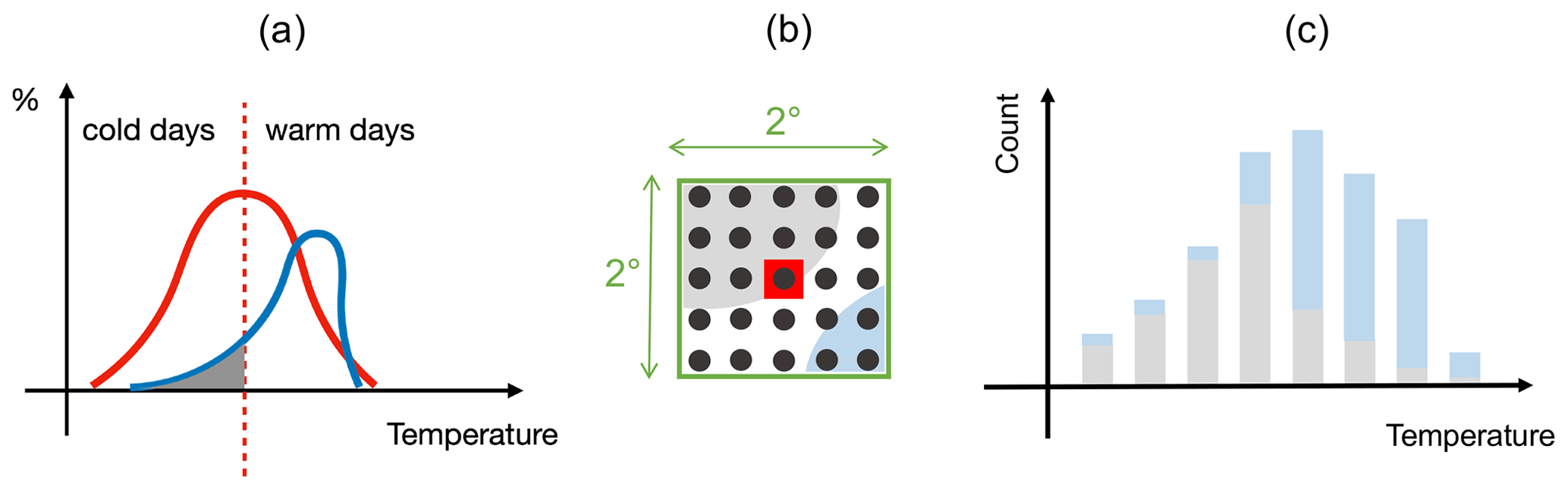
Figure 1Schematics of the methodological aspects. (a) Probability distributions of daily mean 2 m temperature for all days (red) and wet days only (blue) at a particular grid point. The vertical dashed red line denotes the median of the T distribution for all days, and the grey shading marks the fraction of wet days below this median. (b) A box is used to attribute weather systems (grey and blue shading) to precipitation at a grid point (red square). The black points symbolize each grid point in the box. (c) Frequency of occurrence of the blue and grey weather systems as a function of wet day temperature.
2.2 Weather systems
All weather systems are identified as 6-hourly 2D binary fields with the value of 1 at grid points that belong to the weather system and the value of 0 at grid points that do not belong to it. The identification of cyclones, anticyclones, and warm conveyor belts is based on the methods described in Sprenger et al. (2017), and for atmospheric rivers the method of Sodemann et al. (2020) is used. Note that the climatologies of these weather systems were originally computed with ERA-Interim data and have been recalculated with ERA5 for the purpose of this study. The next paragraph briefly describes the main elements of these identification algorithms; further details can be found in the specific references.
Surface cyclones and anticyclones are defined as regions delimited by the outermost closed sea level pressure (SLP) contour. The contour must enclose at least one minimum for cyclones or maximum for anticyclones (Wernli and Schwierz, 2006). Warm conveyor belts are trajectories ascending at least 600 hPa in 2 d from the planetary boundary layer to the upper troposphere near an extratropical cyclone (Madonna et al., 2014). We use 2D binary fields that represent the warm conveyor belt (WCB) ascent, which corresponds to the horizontal envelope of the positions of the WCB trajectories during their ascent between 800 and 400 hPa. This ascent phase is the part of a WCB with the strongest precipitation (Madonna et al., 2014). Atmospheric rivers are identified at grid points where (i) IWV>20 kg m−2 (equivalent to 20 mm) and (ii) IVT>250 kg m−1 s−1. The 2D objects of atmospheric rivers must have a horizontal extension of at least 2000 km and must be poleward of 20∘ N. This definition was used in Sodemann et al. (2020) and agrees with the definition of Ralph et al. (2018).
At every grid point, we attribute what we regard as the dominant weather system to each wet day. Allowing for a small spatial displacement between the weather systems and the precipitation, a box centred around the grid point with intense precipitation is used to quantify the occurring weather systems. The system that covers the largest area of this box is considered as the dominant weather system. As an example, in Fig. 1b, the grey weather system is identified as the dominant one for the wet day at the red grid point. In order to increase the sample size, this attribution analysis is not only performed for the red grid point in Fig. 1b but for all 25 grid points (black points in Fig. 1b) enclosed by the green box. As already mentioned in the “Introduction”, the identified weather systems can co-occur, and their relative contribution to the daily accumulated precipitation cannot be quantified. Hence, our identification of a dominating weather system based on spatial overlap is a strong simplification, and it does not mean that this weather system exclusively led to the intense precipitation. In addition, we neglect remote influences of weather systems that are outside of the box. For example, an extratropical cyclone that is located to the west of the box may still transport moisture to the area of the intense precipitation event, but it is not considered by our simple weather system attribution. Note, however, that the potential influence of remote weather systems can be qualitatively inferred from the composites of the synoptical flow configurations on wet days shown in Sect. 4.2.
The weather system frequencies are analysed as a function of the wet day temperature (Fig. 1c) for the box. We are particularly interested in whether the P(T) relationship differs for wet days attributed to different weather systems. Figure 1c shows such an example, in which the grey weather system is dominating on colder wet days, while the blue weather system is more frequent on warmer wet days. In such a situation, we say that weather systems are relevant for the P(T) relationship, and we introduce a measure called RWSs (abbreviation for relevance of weather systems), which is calculated as follows. First, we compute a histogram like in Fig. 1c, and from this histogram, we calculate for each T bin the percentage of counts (fi) for each weather system, such that . We do this only for 90 % of the wet days in order to avoid very small counts at the tails of the T distribution, i.e. we only consider wet days between the 5th and 95th percentile of the T distribution. Then, we calculate, for each weather system individually, the average f-values across all T bins. With these values, we compute the anomalies of f in each T bin. In a last step, we calculate the RWS value by summing up all absolute f anomalies and multiplying the resulting value by 100. As the RWS value depends on the number of T bins, we divide the RWS value by the number of T bins. If the distribution of f-values is exactly the same for all T bins, then the anomalies are zero for each T bin, and the RWS value, i.e. the sum of all f anomalies, is zero. Hence, in such a situation, the weather systems would not influence the P(T) relationship. However, if RWS reaches a large value, then P(T) differs for different weather systems, and we regard weather systems as relevant for understanding P(T).

Figure 2Fraction of wet days below the median of the local 2 m temperature distribution (WBM measure, see Sect 2.1) in (a) winter (DJF) and (b) summer (JJA). Yellow crosses indicate the locations of the regions analysed later in this study, black contours show wind speed at 300 hPa starting from 25 m s−1 in 5 m s−1 increments, and the green contour marks the climatological sea ice concentration of 50 %. Panels (c) and (d) illustrate the seasonal 95th percentile of daily accumulated precipitation for DJF and JJA, respectively.
2.3 Identification of wettest and driest seasons
At every grid point and separately for winter and summer, the wettest and driest season is identified based on the area-averaged seasonally accumulated precipitation. More specifically, we calculate the seasonally accumulated precipitation at every grid point and then average these values over the box centred at the grid point (green box in Fig. 1b). As we are not interested in very local structures, the box averaging is used to obtain representative values on the scale of 200 km. The season with the maximum seasonal mean value is defined as the wettest season, and the season with the minimum as the driest season. Note that we take into account all days of a season when calculating the seasonal mean and not only precipitation on days with intense precipitation, i.e. wet days. Once the wettest and driest seasons are determined, we can analyse whether these seasons are warmer or colder than normal (i.e. the climatological mean), as well as if, during these anomalous seasons, weather systems occur more or less frequently and/or produce more or less precipitation. Further methodological details are presented at the beginning of Sect. 5.
We start our analysis with the question of whether wet days are predominantly warm or cold (compared to the local climatology) and how this differs regionally and seasonally.
3.1 The winter season (December–February, DJF)
In DJF, in most regions of the extratropical Northern Hemisphere, intense precipitation falls predominately (>80 %) on warmer days, especially at higher latitudes, e.g. in the Arctic, Siberia, northern parts of Canada, and Greenland (Fig. 2a). These areas experience very cold temperatures in winter due to the (partial) absence of incoming solar radiation and the presence of a widespread snow cover. According to the Clausius–Clapeyron relationship, saturation-specific humidity is therefore very low in the high latitude winter, and consequently also the 95th percentile of daily precipitation is low (Fig. 2c). In these regions, a larger amount of precipitation, i.e. the occurrence of a wet day, requires the advection of warmer air with comparatively high specific humidity, which occasionally occurs in the form of moist intrusions (e.g. Bintanja et al., 2020) often associated with extratropical cyclones (e.g. Binder et al., 2017). Hence, it makes sense that wet days in the Arctic are almost exclusively warm.
Over most areas of the North Pacific and the North Atlantic, intense precipitation also falls predominantly on warmer days during winter (Fig. 2a); however, the signal over the North Pacific is more homogeneous compared to the North Atlantic, where the fraction of warm wet days decreases from west to east from about 80 % to 50 %. Hence, the distribution of temperature on wet days and all days is rather similar over the eastern North Atlantic, and therefore, intense rain is equally likely to occur on warm and cold days. Interestingly, there appears to be a correlation between the climatological wind speed at 300 hPa and the wet day frequency on warm days. The maxima of the jet stream over the western North Atlantic and the generally elevated wind speeds over the North Pacific are co-located with areas where intense precipitation is favoured on warmer days. In addition, areas with a high 95th percentile of daily precipitation over the oceans agree with areas where precipitation falls on warmer days (Fig. 2a, c). One plausible explanation for this might be the increased baroclinicity in strong jet stream regions, which (i) is an important prerequisite for cyclone development and (ii) facilitates intense precipitation where southerly (warm) flow is forced to ascend along the comparatively steep isentropes, e.g. in the form of a WCB. As an example, the dark red stripe in Fig. 2a over the western North Atlantic, an area known for its high cyclogenesis frequency (Wernli and Schwierz, 2006), is co-located with a high 95th percentile of daily accumulated precipitation. However, it should be noted that this relationship between upper-level winds and wet day frequency is discernible only in winter (Figs. 2a and S1 in the Supplement, which shows the same analysis for the spring and autumn seasons).
In contrast, the Mediterranean, characterized by an increased cyclone frequency (Wernli and Schwierz, 2006), experiences intense precipitation on colder days (60 %–90 %, Fig. 2a). The wet day threshold is comparatively high (Fig. 2c). The other region with cold wet days is the central US in and downstream of the Rocky Mountains, which was also described in Isaac and Stuart (1992). In contrast to the Mediterranean, the wet day threshold in this area is quite low (Fig. 2c) due to lee effects of the Rocky Mountains. In addition, climatological wind speeds at 300 hPa are low in the vicinity of the Rocky Mountains, as well as over the Mediterranean.
3.2 The summer season (June–August, JJA)
During JJA, most of the wet days are cold in many regions of the extratropical Northern Hemisphere (Fig. 2b). The signal is particularly strong with fraction values exceeding 90 % in regions that are close to very dry summer climates, e.g. southern Europe, regions near the Black or the Caspian Sea, and the western US but also in regions with a wet summer climate, e.g. the eastern US (Fig. 2d). Overall, the contrast between land and ocean is stronger during summer than winter presumably due to the weaker jet stream (Fig. 2b), i.e. the reduced role of baroclinic instability for the formation of precipitation systems and the increased role of continental convection and monsoonal flows that are driven by land–sea contrasts. Other possible factors are surface cold pool formation associated with moist convection, decreased insolation due to increased cloudiness, adiabatic cooling associated with orographic ascent, and the occurrence of precipitation in connection with the passage of weak cold fronts. It is interesting that in many regions over land, in contrast to winter, intense precipitation falls on the colder and not on the warmer days. This implies that high temperatures and a potentially high local moisture availability alone are not sufficient for intense precipitation. A first reason for this is that horizontal moisture transport into the area is relevant for intense precipitation also in the warm season (e.g. Panthou et al., 2014; Grams et al., 2014). In addition, weather systems that occur during warmer days in summer, e.g. blocks and stationary anticyclones, suppress the formation of precipitation due to subsidence (e.g. Zschenderlein et al., 2019). Only the very high latitudes of the North Pacific and the North Atlantic (with fractions of 60 %–70 %), as well as Greenland (>80 %), are characterized by preferentially warm wet days also in summer.
The pattern over the Arctic appears to be strongly influenced by the climatological sea ice extent in both winter and summer (Fig. 2a, b). In winter, the fraction of comparatively warm wet days is particularly high over sea ice, locally exceeding 95 %, which is plausible because precipitation in this area depends on the transport of warm and moist air. In summer, the pattern reverses, and the climatological sea ice extent marks the border between areas where precipitation preferentially occurs on warm days over the North Pacific and North Atlantic and areas with precipitation on (mostly) colder days over the sea-ice-covered Arctic. One possible reason for this pattern is that warmer summer days in the Arctic are accompanied by high-pressure systems that suppress precipitation and increase solar radiation and sea ice melting (Wernli and Papritz, 2018).
3.3 Selected regional analyses
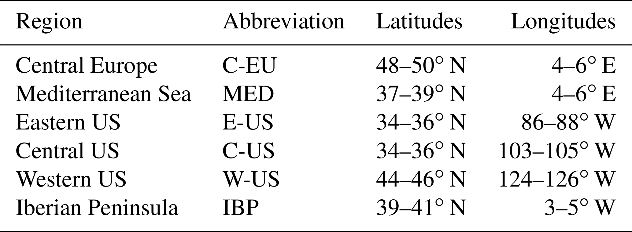
In order to better understand how intense precipitation depends on temperature, we compare the temperature distributions from all days and from wet days for three selected regions in Europe and North America (marked with yellow crosses in Fig. 2a, b; see Table 1 for coordinates and abbreviations) in winter and summer. In all regions, the shape of the overall distribution of daily mean temperatures resembles, as expected, a (skewed) normal distribution with varying means and variances (black line in Figs. 3 and 4). Temperatures are less variable over the Mediterranean Sea (MED) and western US (W-US) compared to all other regions (Figs. 3c, f and 4b, e), and W-US experiences the smallest temperature contrast between summer and winter (Fig. 4b, e). The shape of the temperature distributions in the eastern US (E-US) and central US (C-US) differ substantially between the two seasons; especially E-US has a broad distribution in winter and a narrow one in summer (Fig. 4a, c, d, f). The differing shapes are not only discernible for the whole temperature distribution but also for the temperature distribution on wet days only, in particular for E-US and C-US where the variance is higher in winter compared to summer. In general, the T distributions of all days and of wet days only differ substantially in regions where the fraction values in Fig. 2a and b are either very high or very low, i.e. where wet days are predominantly cold or warm. As an example, more than 80 % of wet days in winter in central Europe (C-EU) are warm (Figs. 2a and 3a), and therefore, the T distributions of all days and wet days differ substantially in Fig. 3a. In agreement with Fig. 2, the deviation of the two T distributions can also change from winter to summer; for example, in the Iberian Peninsula (IBP) in summer most of the wet days are cold (Fig. 3e), but in winter there is a weak shift of the wet days towards warmer days (Fig. 3b).
4.1 The dominating weather systems on wet days

Figure 3P(T, WS) relationships in winter (a–c) and summer (d–f) for the following regions: C-EU (a, d), IBP (b, e), and MED (c, f). The black curve shows the T distribution of all days (right y axis), and the colours in the stacked bar plots denote the dominant weather system on wet days (left y axis). Values denote counts of grid points in the box where a particular weather system is identified as the dominant one. Note the different scaling of the y axis in the different panels. In the upper left of each panel, values are given for the fraction of wet days below the median of daily mean temperatures (WBM; cf. Fig. 2a and b) and the relevance of weather systems for the P(T) relationship (RWS).
Up to this point we have analysed whether wet days are predominantly warm or cold relative to the local T climatology. In this section, our objective is to identify the weather systems that occur on wet days and, more specifically, on colder vs. warmer wet days. To this end, Figs. 3 and 4 depict, for the same regions as discussed in the previous subsection, distributions of the dominant weather systems on wet days as a function of temperature in winter and summer, as well as the weather system relevance measure RWS introduced in Sect. 2.2. We recall that the weather systems considered are extratropical cyclones, warm conveyor belts, atmospheric rivers, and anticyclones (potentially with convection) and that with our approach we identify for each wet day a single “dominant weather system”. For details of this approach, see Sect. 2.2.
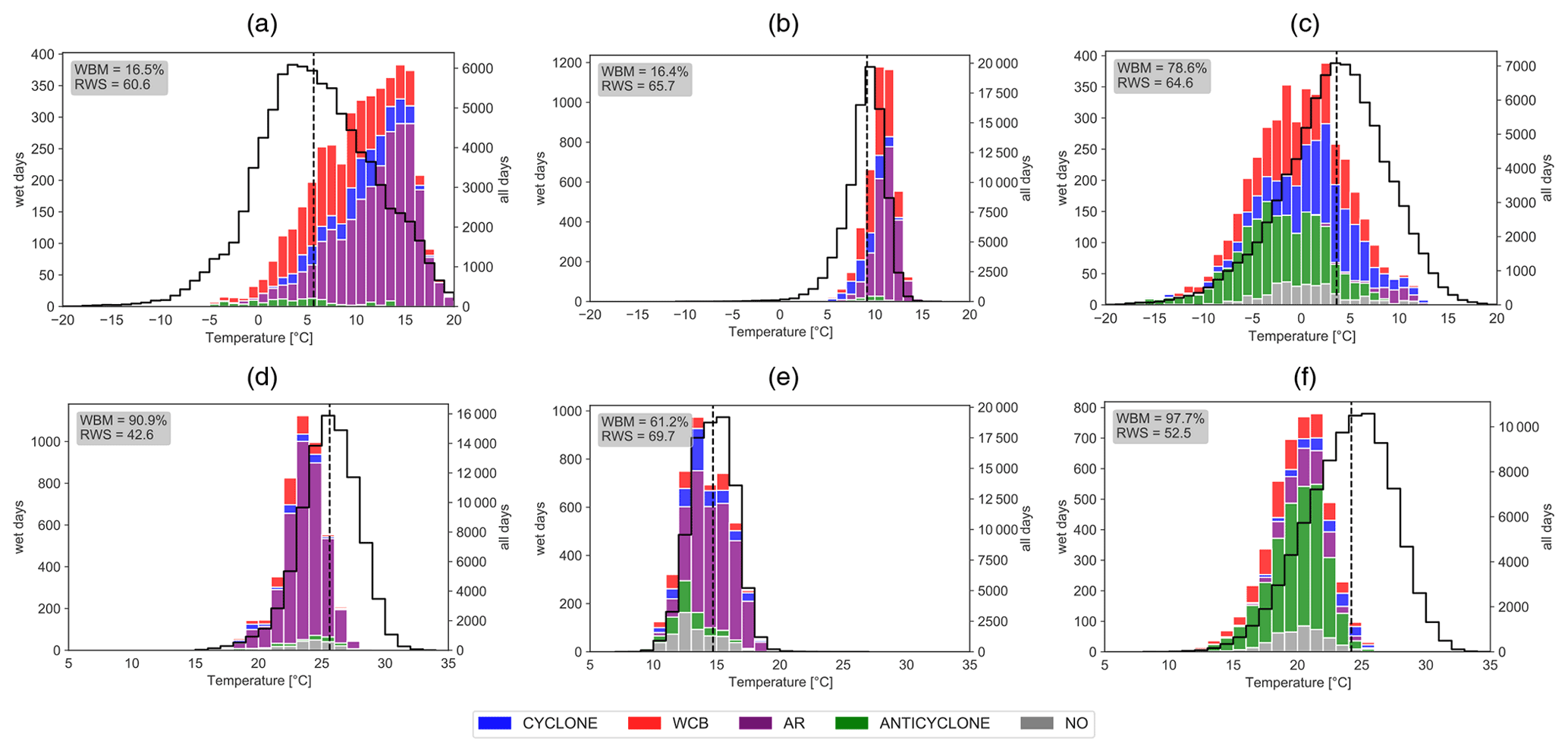
Figure 4Same as Fig. 3 but for three regions in North America: E-US (a, d), W-US (b, e), and C-US (c, f).
We first consider the three European regions (Fig. 3). In winter over C-EU and IBP, in which wet days are predominantly warm (Fig. 2a), warm conveyor belts are most frequent on wet days, followed by cyclones and atmospheric rivers (Fig. 3a, b). Only on a very few wet days (2.6 %) do none of the considered weather systems occur in the region, and they were attributed to the category “NO”. Cyclones are dominating on colder wet days, warm conveyor belts on moderately warm days, and atmospheric rivers on the warmest wet days. Hence, the weather systems strongly influence the P(T) relationship, and this is reflected in RWS values of 78.3 for C-EU, which is the highest for all regions, and 68.1 for IBP (Fig. 3a, b). In contrast, in MED, cyclones dominate on most wet days independently of T (Fig. 3c), and the RWS value is 44.4, indicating a smaller influence of weather systems on the P(T) relationship compared to C-EU and IBP. In MED, wet days are typically cold (80 %, Figs. 3c and 2a). Warm conveyor belts contribute to some wet days in the intermediate T-range, whereas atmospheric rivers in a few cases dominate on warm wet days. Anticyclones are very rarely associated with wet days in all three regions.
In summer, when wet days are mostly cold in all three regions (Figs. 2b and 3d–f), the frequency and T distribution of weather systems change in all regions. Over C-EU, atmospheric rivers dominate (Fig. 3d), over IBP cyclones do (Fig. 3e), and over MED no weather system is clearly dominating (Fig. 3f). Note that the wet day threshold in MED in summer is very low (Fig. 2d) such that some of the considered wet days are not associated with large amounts of precipitation. Compared to winter, a relatively large fraction of wet days cannot be assigned to a weather system, in particular in MED and IBP (labelled with “NO” in Fig. 3). We assume that precipitation on these days is related to mesoscale convective processes that frequently occur in summer in these regions, but they are not attributed to our weather systems if they are not located within a well-defined anticyclone. Generally, the influence of weather systems on the P(T) relationship in these regions is weaker in summer than in winter, which is reflected in lower RWS values (Fig. 3d–f).
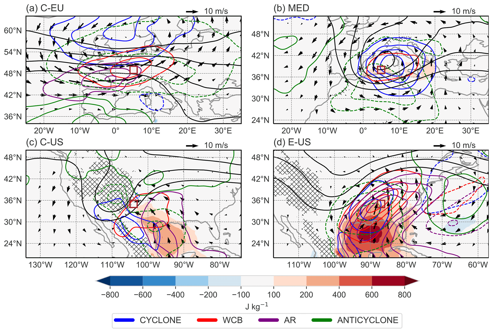
Figure 5Composites for wet days in winter in the regions (a) C-EU, (b) MED, (c) C-US, and (d) E-US. Coloured contours show frequency anomalies of cyclones (blue), warm conveyor belts (red), atmospheric rivers (purple), and anticyclones (green) for values of −40 %, −30 %, −20 %, −10 %, 10 %, 20 %, 30 %, and 40 % (dashed lines for negative values). The arrows mark the anomalous wind at 850 hPa. The black line illustrates upper-level PV at 320 K, starting from 2 pvu in 1 pvu increments. Colour shading denotes anomalies of daily maximum CAPE, and the hatching marks altitudes of 1500 m. All anomalies are calculated with respect to the seasonal mean climatology. The contours of the weather features have been smoothed with a Gaussian filter.
Considering now the three regions in North America (Fig. 4), the distribution of weather systems on wet days in winter is similar for W-US as for C-EU and IBP but with more atmospheric rivers and fewer cyclones (Fig. 4b). In these regions, wet days are warm in winter (Fig. 2a). Over E-US, where wet days are also typically warm (Fig. 2a), atmospheric rivers are also very frequent on wet days; however, warm conveyor belts dominate on colder and moderately warm wet days (Fig. 4a). Over C-US, the contribution of weather systems is rather complex. We recall that wet days are typically cold in this region (Figs. 2a and 4c). Anticyclones dominate on colder wet days and warm conveyor belts and cyclones on warmer wet days (Fig. 4c). However, for some wet days with moderately warm temperatures no weather system could be assigned to precipitation, which implies that other processes, for instance orographic effects, can lead to intense precipitation. Overall, in all regions, weather system frequencies depend on T and are therefore important for the P(T) relationship with RWS values between 60 and 65 (Fig. 4a–c).
In summer, when, as over Europe, most wet days are cold (Fig. 2b), E-US and W-US are largely dominated by atmospheric rivers (Fig. 4d, e), while anticyclonic situations mainly prevail in C-US (Fig. 4f). For both E-US and C-US, RWS values are smaller than in winter, while for W-US, the RWS value is slightly larger. Hence, the relevance of weather systems on the P(T) relationship increases for W-US, while it decreases for E-US and C-US. Interestingly, fewer summer wet days could not be attributed to one of the four weather systems in North America than in Europe (compare Figs. 3d–f and 4d–f).
The general pattern that appears in winter in C-EU and IBP is that warm conveyor belts and atmospheric rivers dominate more on warmer wet days, whereas cyclones do more on colder wet days. This appears intuitive because warm conveyor belts and atmospheric rivers occur preferentially in the warm sector of the cyclone. Hence, precipitation on colder wet days is then likely related to shallow convection in the cold sector of a cyclone and/or precipitation from the cloud head near the cyclone centre. An interesting result is that anticyclones are frequently associated with intense precipitation in C-US in both seasons (Fig. 4c, f). Plausible reasons for this result are (i) flow interactions of the anticyclones with the Rocky Mountains (e.g. a persistent, moist, and upslope flow), (ii) locally embedded thunderstorms (in particular in summer), and (iii) large-scale ascent that is often observed along the western edge of anticyclones (e.g. Zschenderlein et al., 2020). In order to better understand the role of the involved weather systems, their potential interaction, and the general large-scale flow conditions, we now look at the synoptic environments on the wet days.
4.2 Composites of weather systems on wet days
Figures 5 and 6 show composites for days when the wet day threshold (95th percentile of daily precipitation) was exceeded at least at 50 % of the grid points in the considered region. From the regions analysed in Sect. 4.1, we selected two regions each in Europe and North America such that they represent the regional weather system variability revealed in Figs. 3 and 4. The composites for the other regions are shown in the Supplement (Figs. S2 and S3). Since composites show mean conditions and do not consider the variability in the underlying synoptic flow configurations, it is interesting to analyse this variability. For example, the question could be answered of whether a wet day dominated by a cyclone is associated with a different flow configuration than a wet day dominated by an atmospheric river. For that, we identify wet days dominated by a particular weather system (i.e. cyclone, anticyclone, warm conveyor belt, atmospheric river) and show composites for each weather system individually (Figs. S4–S6). These composites are only shown for regions characterized by a high synoptic flow variability on wet days; for the other regions, the overall composites in Figs. 5 and 6 can be considered as representative for all wet days. Anomalies in Figs. 5, 6, and S2–S6 are calculated with respect to the seasonal mean climatology, which incorporates all days during DJF and JJA 1980–2019.
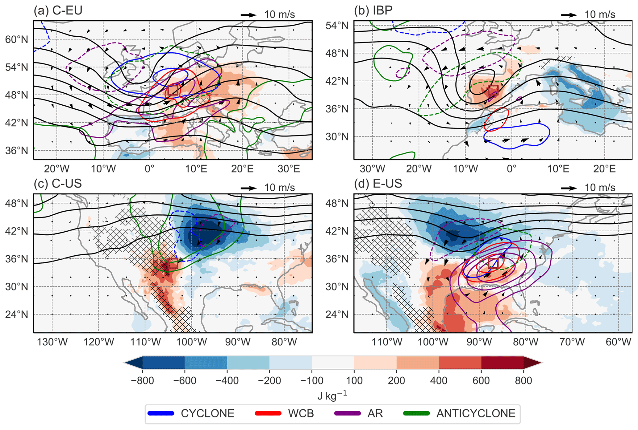
Figure 6Same as Fig. 5 but for wet days in summer in the regions (a) C-EU, (b) IBP, (c) C-US, and (d) E-US. The black contours denote PV at 340 K.
4.2.1 Winter
Winter wet days in C-EU are associated with intense zonal flow conditions throughout the troposphere with an increased frequency (compared to climatology) of cyclones north and anticyclones south of the precipitating area (Fig. 5a). The large-scale weather pattern resembles the positive phase of the North Atlantic Oscillation (Hurrell et al., 2003). Recall that wet days in this region occur on climatologically warmer days (Fig. 3a) most likely due to advection of mild (and humid) air from the North Atlantic. Atmospheric rivers frequently occur southwest of the precipitation area, while enhanced warm conveyor belt frequencies are found centred around the precipitation area. This strong co-location explains the dominance of warm conveyor belts in Fig. 3a. The shift in the frequency maxima of atmospheric rivers and warm conveyor belts is in line with the classical situation of warm conveyor belts rising from very humid low-tropospheric regions at the end of atmospheric rivers (see, for example, the schematic Fig. 2.8 in Sodemann et al., 2020). Similar composite results are found for IBP and W-US (Fig. S2), with the main differences being that in these regions the potential vorticity (PV) trough is more pronounced and the positive cyclone anomaly is more upstream. These regions also had similar P(T, WS) diagrams (compare Figs. 3a, b, and 4b). The synoptic flow configuration in Fig. 5a is dominated by wet days associated with warm conveyor belts (Fig. S4a); however, 22 % of wet days in C-EU are dominated by atmospheric rivers. On these days, anomalous 850 hPa winds are more zonally oriented compared to wet days with warm conveyor belts, and stronger positive anticyclonic anomalies are found south of C-EU (Fig. S4b). On 19 % of wet days in C-EU, cyclones are dominating, which is associated with cyclonic wind anomalies, a slightly stronger PV trough, and decreased warm conveyor belt and atmospheric river frequencies (Fig. S4c).
In contrast to C-EU, winter wet days in MED (which occur on colder days, Fig. 3c) are associated with a clear cyclonic wind anomaly in the lower troposphere, and cyclones occur frequently very close to the precipitation area (Fig. 5b). This agrees with the high frequency of cyclones in Fig. 3c and with the fact that the Mediterranean is a hotspot for the co-location of cyclones and intense precipitation events (Hawcroft et al., 2012; Pfahl and Wernli, 2012; Catto and Dowdy, 2021; Messmer and Simmonds, 2021; Owen et al., 2021). The influence of warm conveyor belts is considerably reduced, and atmospheric rivers are negligible, in agreement with the low climatological frequency of these features in the Mediterranean.
As already seen in Fig. 4c, wet days in C-US are influenced by anticyclonic conditions, and they also occur on colder days. Indeed, Fig. 5c reveals an increased anticyclone frequency anomaly northeast and an increased cyclone frequency anomaly southwest of C-US, which favours an anomalous lower-tropospheric easterly wind directed towards the Rocky Mountains. Thus, orographic effects influence the formation of intense precipitation in this area. The upper-level PV trough supports the formation of cyclones in the lee of the Mexican Sierra Madre. Interestingly, CAPE values are anomalously high over the Gulf of Mexico, and the anomalous southeasterly wind is directed from higher to lower CAPE values. Therefore, the orographic ascent can be associated with embedded convection. The southeasterly wind on wet days was already described by Hobbs et al. (1996) and interpreted as a low-level jet transporting moist and warm air northward. Hobbs et al. (1996) found that the convergence of subsiding air off the Rocky Mountains, which is warm and dry, and of warm and moist air transported northwards from the Gulf of Mexico can lead to a narrow zone of strong moisture gradients – a dryline. If the dryline co-occurs with a lee trough, convective precipitation and thunderstorms can develop (Hobbs et al., 1996). The pattern in Fig. 5c resembles the occurrence of cold surges along the Rocky Mountains, which involve cold air damming and a strongly sloping baroclinic zone (Colle and Mass, 1995). Recall that wet days are typically cold in this area; hence, air advected with the low-level jet is presumably less warm than during westerly wind conditions when foehn effects lead to even warmer temperatures but dry conditions. It is also noteworthy that the 850 hPa flow direction in the C-US box and the direction of the upper-level flow, indicated by the PV contours, are almost opposite, indicating a strong thermal wind and hence a strong meridional temperature contrast across the region. Interestingly, wet days in C-US are characterized by a high synoptic flow variability. Wet days dominated by cyclones or warm conveyor belts are associated with a PV trough and anomalously high CAPE values southeast of the box (Fig. S5a and c). However, 34 % of wet days in C-US are dominated by anticyclones (Fig. S5b). On these days, anticyclones occur in the lee of the Rocky Mountains downstream of a tilted upper-level PV trough, and at 850 hPa, easterly wind anomalies prevail. In addition, no anomalous CAPE values can be observed in the vicinity of the box (Fig. S5b).
In E-US, wet days occur ahead of an upper-level PV trough (Fig. 5d), which leads to strong southerlies transporting moist and warm air northwards from the Gulf of Mexico. Cyclones and warm conveyor belts are located ahead of the PV trough. Due to the high moisture transport, atmospheric rivers extend from the Gulf of Mexico across the southeastern and eastern US. Positive frequency anomalies of cyclones, warm conveyor belts, and atmospheric rivers are almost co-located. The synoptic situation resembles the synoptic flash flood type in Maddox et al. (1979) and agrees with extreme precipitation events in the southeastern US driven by a pronounced upper-level trough and a steady southerly corridor of strong water vapour transport (Moore et al., 2015). CAPE values are strongly enhanced over the Gulf of Mexico and still slightly in the E-US box.
4.2.2 Summer
Figure 6 presents the composites for summer and reveals interesting differences to winter. In C-EU, intense precipitation occurs ahead of an upper-level PV trough and under weak cyclonic lower-tropospheric wind anomalies (Fig. 6a). Cyclones are now closer to the precipitating area, which explains the higher numbers of cyclones compared to winter (Fig. 3a, d). Another obvious difference to winter is the anomalously high CAPE values, which are generally increased over all regions considered. The composite for W-US is qualitatively similar to the one for C-EU but with more atmospheric rivers and negligible CAPE values (Fig. S3b). The composites for the two Mediterranean regions IBP and MED reveal the influence of an upper-level trough and weak cyclonic wind anomalies and, in particular for IBP, anomalously high CAPE values (Figs. 6b and S3a). Note that over IBP cyclone frequencies are only slightly increased compared to climatology (by less than 10 %) and are therefore not visible in Fig. 6b.
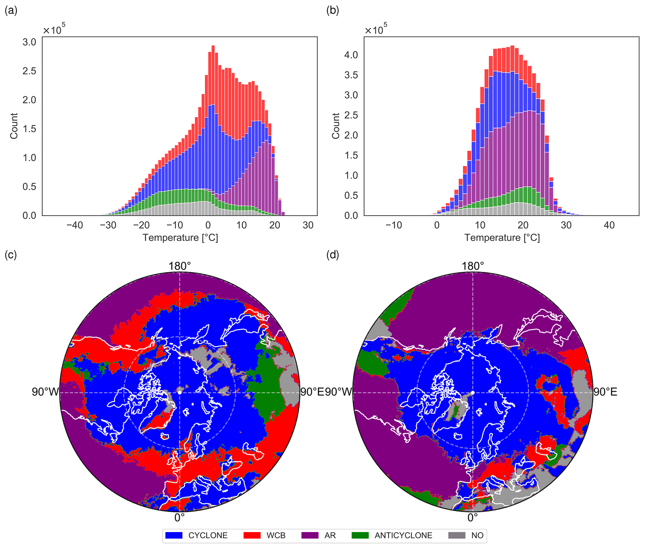
Figure 7The colours in the stacked bar plots denote the dominant weather system on wet days and for all grid points from 30 to 60∘ N in DJF (a) and JJA (b). The lower row shows the dominant weather system of all wet days in DJF (c) and JJA (d).
In C-US, in sharp contrast to winter, large-scale forcing is weak in summer, and convective and orographic processes seem to dominate (Fig. 6c), in agreement with Fig. 4f. The weak upper-level ridge induces an anticyclonic circulation directed towards the Rocky Mountains. Similar to winter, wet days in C-US are also characterized by a high variability in the synoptic flow. Although 54 % of wet days are dominated by anticyclones, 13 % of wet days are dominated by atmospheric rivers and 13 % by warm conveyor belts (Fig. S6). Wet days that are dominated by atmospheric rivers are characterized by a weak upper-level PV trough upstream and over the Rocky Mountains and weak southerly wind anomalies at 850 hPa, together with enhanced atmospheric river frequencies and enhanced CAPE values (Fig. S6b). On wet days dominated by warm conveyor belts, northeasterly 850 hPa wind anomalies are weak, but high CAPE values occur in the C-US region (Fig. S6c). No frequency anomalies of anticyclones occur on wet days dominated by warm conveyor belts or atmospheric rivers (Fig. S6b, c).
Over E-US, upper-level forcing is also weaker compared to winter, which is reflected in weaker lower-tropospheric wind anomalies (Fig. 6d). The weaker upper-level forcing and higher CAPE are typical for this season and region (Moore et al., 2015). Interestingly, E-US is located between a dipole of anomalously low CAPE values north and high CAPE values south of the precipitation area. The weak southwesterlies transport warm and humid air towards E-US, which is reflected in enhanced atmospheric river frequencies directed from the Gulf of Mexico towards the target area. Note that in this region in summer, wet days are typically cold (Fig. 4d), and therefore, air advected from the Gulf of Mexico is still less warm than air that is either transported from the inner continent or descending in an anticyclone, which leads to warm but dry conditions.
In summary, considering both winter and summer, the wet day composites reveal for most regions a variant of the flow situation with an upper-level trough, a westerly or southwesterly moist flow often identified as an atmospheric river, and a surface cyclone either above the precipitation region or further northwest or north with a warm conveyor belt directly above the precipitating region. Interestingly, this archetypal flow configuration occurs mainly in regions and seasons in which intense precipitation occurs on warmer days but also in winter in MED and in summer in C-EU and E-US where intense precipitation occurs on colder days. This indicates that the weather system constellation is not a direct indication for whether wet days are primarily cold or warm. Very different composites were found for C-US where the flow interaction with topography appears to be essential for the occurrence of wet days in both seasons.
4.3 Global analysis of P(T, WS)
Up to this point we have quantified how weather systems influence the P(T) relationship in selected regions. In order to increase the validity of our findings, we repeat the analysis leading to the results shown in Figs. 3 and 4 at all grid points between 30 and 60∘ N (Fig. 7). Because in summer the 95th percentile of total precipitation can be very low, we excluded wet days with precipitation below 1 mm in Fig. 7b. In winter, wet days with T<0 ∘C are dominated by co-located cyclones, and with T between 0 and 10 ∘C through warm conveyor belts and with T above 10 ∘C, atmospheric rivers are predominantly identified as the dominant weather system (Fig. 7a). The relative fraction of anticyclones and wet days not assigned to a weather system is higher for very cold wet days below −10 ∘C (Fig. 7a). In summer, atmospheric rivers occur more frequently in the entire T distribution (Fig. 7b); hence, the results of the regional analysis (Figs. 3 and 4) are qualitatively similar to the mid-latitude analysis except for C-US (Fig. 4c) where anticyclones occur more frequently.
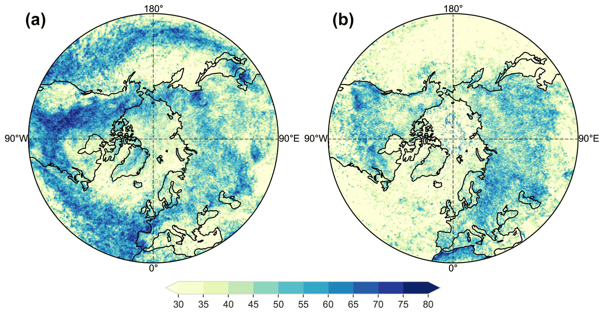
Figure 8Relevance of weather systems (RWSs) for the P(T) relationship in DJF (a) and JJA (b).
Figure 7a revealed that atmospheric rivers occur frequently on warmer wet days during winter. It therefore makes sense that atmospheric rivers are often co-located with wet days in climatologically warmer areas, e.g. in the southern part of the storm tracks of the North Atlantic and North Pacific (Fig. 7c). Warm conveyor belts dominate wet days in Europe and most parts of western North America, while cyclones occur frequently in the Mediterranean and in climatologically colder regions of Eurasia and North America (Fig. 7c). Anticyclones occur frequently on wet days in climatologically dry areas near mountains, e.g. the Rocky Mountains and the Himalayas (Fig. 7c). In summer, the influence of atmospheric rivers on wet days increases in many areas of the extratropics (Fig. 7b, d), which is in qualitative agreement with the regional analyses (Figs. 3d–f and 4d–f) and the climatologically higher frequency of atmospheric rivers in the extratropics (Sodemann et al., 2020). Areas where cyclones and warm conveyor belts are dominating on wet days are smaller compared to those in winter. In general, the contribution of anticyclones to intense precipitation, potentially with convection, as described for C-US (Figs. 4f and 6c), is climatologically quite seldom in summer (Fig. 7d). In the Mediterranean, intense precipitation can mostly not be assigned to a weather system (Fig. 7d), which indicates that intense precipitation in this region occurs in situations with, for example, weak pressure gradients and lower-tropospheric instability that can lead to localized showers and thunderstorms.
We have seen in Figs. 3 and 4 that the influence of weather systems on the P(T) relationship varies between the regions and seasons; therefore, we repeated this analysis for all grid points of the extratropical Northern Hemisphere (Fig. 8). It can be deduced from the regional analysis in Figs. 3 and 4 that RWS values above 50 are an indicator that considering weather systems is relevant for understanding the P(T) relationship, i.e. that P(T) differs substantially for individual weather systems. In winter, an RWS value of 50 is exceeded in the storm track regions of the North Pacific and North Atlantic, as well as over large parts of the North American continent east of the Rocky Mountains and parts of central and western Europe (Fig. 8a). In summer, when upper-level winds are weaker than in winter (Fig. 2a, b), the overall relevance of weather systems for the P(T) relationship decreases, in particular in the North Pacific and North Atlantic but also in parts of North America and Europe. Hence, the P(T) relationship is less influenced by the frequencies of weather systems in this area, which was already indicated by the regional analysis (Figs. 3d–f and 4d–f). Only in some locations are weather systems more relevant for the P(T) relationship in summer than in winter, e.g. in areas upwind of the Rocky Mountains or in western Russia (Fig. 8b). In summary, the influence of weather systems on the P(T) relationship appears to be particularly strong in regions with strong upper-level winds and therefore increased baroclinicity, especially in winter. However, the relevance of weather systems for the P(T) relationship does not depend on the preference of wet days to occur on warm or cold days (compare with Fig. 2a, b) nor on the wet day threshold (see Fig. 2c, d). In general, the variability in P(T) for different weather systems, as measured by our relevance metric RWS, is large in most regions of the extratropics, indicating that studying the P(T, WS) relationship is meaningful and important. Exceptions are regions where a single weather system dominates wet days at all temperatures, which happens, for example, with cyclones in the Arctic and in winter in the Mediterranean.
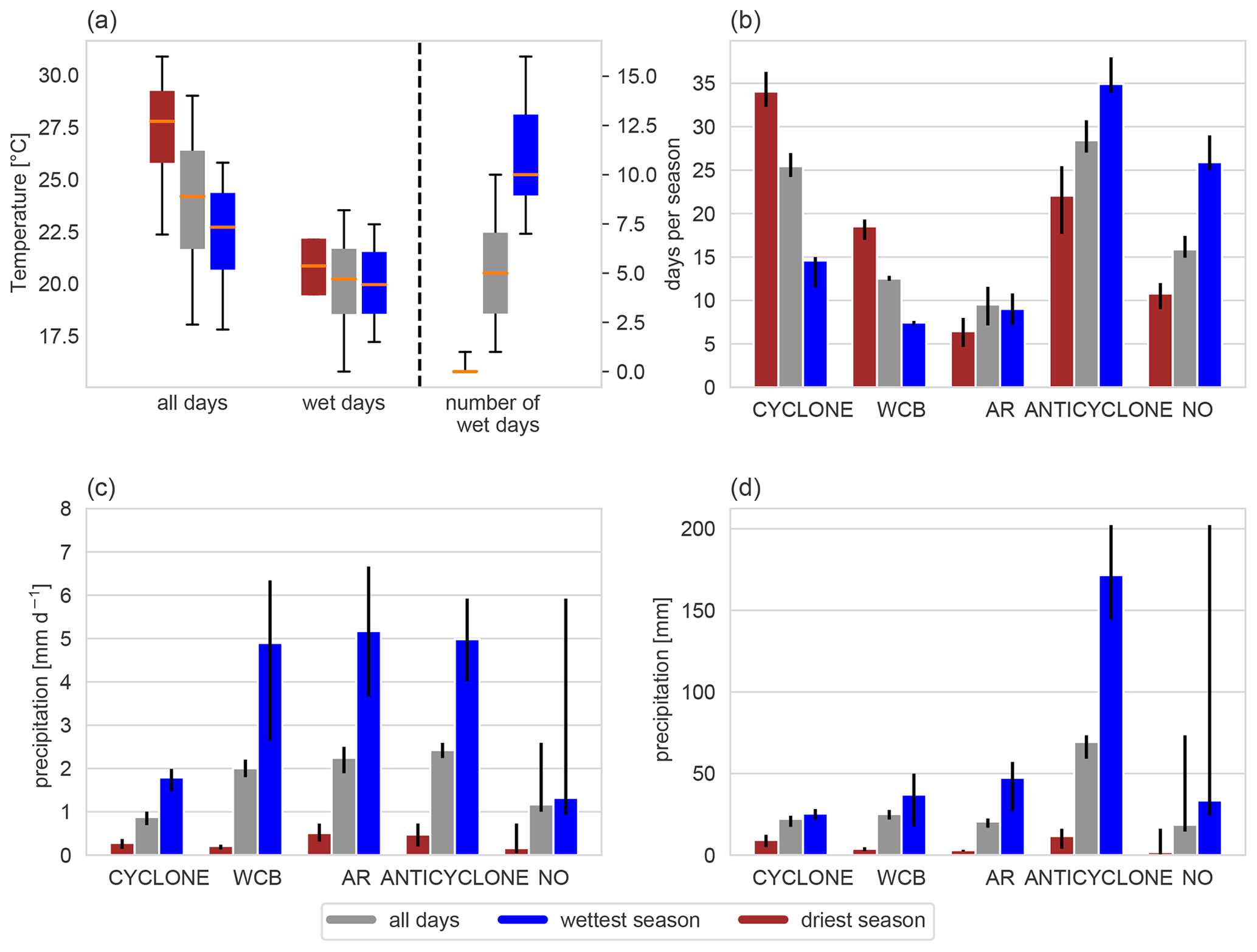
The final part of this study considers the seasonal timescale and investigates how the frequency and precipitation efficiency of weather systems change in anomalously wet and dry seasons. For this analysis, we focus on C-EU, where wet days are warm in winter and cold in summer and essentially driven by cyclones, warm conveyor belts, and atmospheric rivers (Fig. 3a, d), and on C-US, where wet days are cold in both seasons and strongly influenced by surface anticyclones (Fig. 4c, f).
We first compare the temperature distribution on all days for the climatology with the anomalous seasons (e.g. Fig. 9a, left), as well as the total number of days when a weather system is present in the region (e.g. Fig. 9b) and the weather systems' precipitation efficiency (e.g. Fig. 9c), again for all vs. the wettest and driest seasons. The number of days with a weather system is calculated as follows. First, we count the number of days a weather system overlaps with a region (green box in Fig. 1b). If weather systems occur simultaneously, as for example in the schematic example in Fig. 1b, the weather systems are treated as if they had occurred for only half a day. If all four weather systems occur simultaneously, each system is counted as if they had occurred for only a quarter of a day. In order to increase the sample size, we repeat this procedure for all 25 grid points in the region (black points in Fig. 1b), similar to Sect. 2.2. The resulting frequencies are shown as days per season (e.g. Fig. 9b). This approach enables us to quantify the contribution of each weather system to the total seasonal precipitation (e.g. Fig. 9d). The precipitation efficiency, i.e. the daily precipitation rate per weather system, is calculated for each weather system individually as the average precipitation on days when the weather system occurred in the region (e.g. Fig. 9c). Also this procedure is repeated for all 25 grid points.

Figure 9Seasonal analysis for C-EU in winter. (a) T distributions for all days and wet days only, as well as number of wet days, (b) mean weather system frequency on all days, (c) mean weather system precipitation efficiency, and (d) total precipitation associated with each weather system category. The colours denote results for the climatology, i.e all days (grey) and for the wettest (blue) and the driest winter (red). In (a), the orange line denotes the median, the box values are between the 25th and 75th percentiles, and the whiskers extend from the 5th to the 95th percentile. Black error bars in (b)–(d) denote the inter-quartile range of the 25 grid points in the box.
5.1 C-EU in winter
In C-EU in winter, anticyclones are climatologically the most frequent weather systems, followed by warm conveyor belts, days with no weather system, cyclones, and atmospheric rivers (grey bars in Fig. 9b). Note that in contrast to the previous sections, the frequency is calculated for all days and not only for wet days with accumulated precipitation above the 95th percentile. Although atmospheric rivers occur relatively seldom, they are associated with the highest precipitation intensity of about 7 mm d−1 (grey bars in Fig. 9c), while both days with anticyclones and days without a weather system have very little precipitation on average (Fig. 9c). The contribution of each weather system to the seasonal accumulated precipitation, i.e. the product of Fig. 9b and c, shows that warm conveyor belts are usually contributing by far the largest fraction to the seasonal precipitation in this region (Fig. 9d).

The wettest winter in C-EU occurred in 1994/95 with around 420 mm of accumulated precipitation, which is almost twice the climatological amount. This winter had an average temperature of 5.1 ∘C and was therefore 2.1 K warmer than climatology. In Fig. 9a on the left, this can be seen as a clear shift in the daily mean temperature distribution towards warmer temperatures. The wettest winter is marked by more and warmer wet days than climatology (Fig. 9a, central and right). Warm conveyor belts and atmospheric rivers occur more frequently, while cyclones, anticyclones, and days without a weather system occur less frequently (Fig. 9b). All weather systems are more efficient during the wettest winter, especially cyclones (Fig. 9c). One reason for the increased precipitation efficiency might be the shift to warmer wet days in this winter (Fig. 9a). Accumulated over the whole winter 1994/95, warm conveyor belts and atmospheric rivers contribute most to the precipitation, and these two weather system categories are to a large part responsible for the extreme precipitation total (Fig. 9d, compare blue and grey bars). In the previous sections where we focused on the daily timescale, we found that for wet days, which are typically warmer (Fig. 2a), warm conveyor belts and atmospheric rivers are dominating (Fig. 3a), while cyclones are more relevant on less warm wet days (Fig. 3a). This relationship appears to have an impact also on the seasonal timescale, i.e. more warm conveyor belts and atmospheric rivers and fewer cyclones, together with generally warmer temperatures during the wettest winter. As already discussed in the previous section, warm conveyor belts and cyclones are always connected to each other. Hence, the lower number of days with cyclones in C-EU during the wettest winter implies that cyclones may take a slightly different track and therefore overlap less frequently with C-EU.
The driest winter in C-EU, which occurred in 2016/17, registered about 90 mm of accumulated precipitation and therefore less than half of the climatological precipitation. It is slightly colder than normal seasons (Fig. 9a) and marked by, as expected, fewer wet days, and these few days are colder than normal (Fig. 9a). The signal in the frequency of weather systems is quite clear, i.e. fewer cyclones, warm conveyor belts, and atmospheric rivers and more anticyclones (Fig. 9b). Overall, most of the weather systems also lead to less daily precipitation and are therefore less efficient except for cyclones, which are even slightly more efficient than climatologically expected (Fig. 9c). The majority of the seasonal precipitation is still attributed to warm conveyor belts; however, the amount is substantially lower than in the climatology (Fig. 9d). Interestingly, atmospheric rivers contribute only very little to the seasonal precipitation, which is presumably related to the slightly colder temperatures in the driest season.
5.2 C-EU in summer

We now continue with the anomalous summers in C-EU. Climatologically, atmospheric rivers occur more often in summer compared to winter (Figs. 9b and 10b) but are less efficient (Fig. 10c), while warm conveyor belts occur less frequently (Fig. 10b) but are nearly equally efficient (Fig. 10c). The seasonal precipitation is predominantly associated with atmospheric rivers, followed by warm conveyor belts and cyclones (Fig. 10d). The wettest summer occurred in 1987 with about 330 mm compared to 200 mm precipitation in the climatology and is marked by colder than average temperatures, more frequent wet days, and also colder wet days (Fig. 10a). Both cyclones and atmospheric rivers occur more often than in normal seasons and warm conveyor belts less often, but all are more efficient during the wettest summer (Fig. 10b, c). The majority of the seasonal precipitation is related to atmospheric rivers and cyclones (Fig. 10d). Warm conveyor belts are less relevant compared to winter because they in general occur less frequently in summer (Madonna et al., 2014). The driest summer occurred in 2018 with about 120 mm precipitation and is marked by fewer wet days and generally higher temperatures on all and on wet days (Fig. 10a). The driest season is characterized by fewer cyclones, warm conveyor belts, atmospheric rivers, and interestingly also anticyclones but with more days without a weather system. It is hypothesized that these days are associated with a flat SLP distribution that is not captured by any of our weather systems. All weather systems are less efficient except for warm conveyor belts (Fig. 10c). Warm conveyor belts contribute most to the total seasonal precipitation, in contrast to the wettest summer, followed by cyclones, atmospheric rivers, days with no weather system, and anticyclones (Fig. 10d).
5.3 C-US in winter
We now compare the results for C-EU with C-US, where wet days are cold in both winter and summer (Fig. 2a, b). C-US in winter is affected by more cyclones than C-EU but with less warm conveyor belts and nearly no atmospheric rivers (Fig. 11b). However, all weather systems are less efficient than in C-EU (Fig. 11c); i.e. they produce less precipitation in this climatologically drier region (Fig. 2c). The wettest winter in C-US occurred in 1986/87 with about 170 mm compared to 60 mm precipitation in the climatology, and it was colder than normal with colder wet days but very frequent wet days (Fig. 11a). The frequency of weather systems does not substantially change compared to normal seasons, and therefore, the strongly increased precipitation efficiency of all weather systems, apart from atmospheric rivers which are negligible in this region, contribute to the wettest winter. Warm conveyor belts, anticyclones, and cyclones are all important for the total seasonal precipitation (Fig. 11d). Interestingly, the category “NO” weather system is also substantially influencing the seasonal precipitation, which implies that some precipitation is related to smaller-scale processes, e.g. convection that cannot be identified with our large-scale weather systems. In comparison to C-EU, the contrast between the wettest and the driest winter is very large – the driest winter, which occurred in 2005/06, measured only about 5 mm accumulated precipitation, which is also the reason why no wet day was identified (Fig. 11a). Similar to the wettest winter, the frequencies of all weather systems are not substantially different from climatology (Fig. 11b); however, all are very dry (Fig. 11c). Hence, whether a winter in C-US is anomalously wet or dry appears to be primarily determined by a change in the precipitation efficiency of weather systems and not by their frequency.
5.4 C-US in summer
In comparison to C-EU in summer, cyclones occur climatologically more frequently and atmospheric rivers less frequently in C-US (Fig. 12b), and cyclones, warm conveyor belts, and atmospheric rivers are less efficient and anticyclones more efficient (Fig. 12c). In contrast to C-EU in both seasons and to C-US in winter, anticyclones play a more dominant role for the seasonal precipitation (Fig. 12d), which is obvious for the wettest summer (Fig. 12d), which occurred in 1984 and registered about 315 mm rain compared to 155 mm in the climatology. Temperatures on all days in the wettest summer are colder than normal; however, wet days are only marginally colder than wet days in normal seasons (Fig. 12a). Although the frequencies of all weather systems change for the anomalous seasons (Fig. 12b), the precipitation efficiency appears to be the driving factor for the precipitation anomaly (Fig. 12c). For instance, cyclones, warm conveyor belts, and atmospheric rivers occur less frequently; however, because the precipitation efficiency is substantially increased, they contribute more to the seasonal precipitation than in normal seasons (Fig. 12d). Overall, the influence of anticyclones and the “NO” system category is strongest for the total seasonal precipitation in the wettest season (Fig. 12d). The driest summer in 2011 with only about 30 mm rain is warmer than normal, and the very few wet days are slightly warmer than normal (Fig. 12a). Similar to the wettest season, the frequencies of some weather systems change (Fig. 12b), but they are all very dry (Fig. 12c, d). Hence, the anomalous seasons in C-US in summer are also largely determined by an increase or decrease in the precipitation efficiency, similar to winter.
The co-variability in daily and seasonal mean surface temperature and precipitation has received much attention in recent years, but the role of weather systems in this relationship has not been investigated yet. We therefore first quantified whether wet days (days with precipitation above the 95th percentile) are predominantly warm or cold and then examined the relative frequencies of weather systems on these wet days as a function of temperature. We applied this methodology to a 39-year ERA5 climatology and to selected regions for studying processes during the wettest and driest seasons. We briefly summarize the results of our study by addressing our research questions.
-
Does intense precipitation typically occur on the colder or on the warmer days of a season?
Intense precipitation in winter in most regions occurs predominantly on warmer days, especially at high latitudes, whereas in the Mediterranean area and central US, intense precipitation falls predominantly on colder days. In summer, intense rain falls mostly on colder days, especially in areas close to dry summer climates, e.g. in the latitude band 35–45∘ N over Eurasia, but also in humid summer climates like the eastern US. Only the high latitudes of the North Pacific and North Atlantic are dominated by intense precipitation on warmer days also in summer.
-
Which weather systems occur preferentially on days with intense precipitation, and do some weather systems typically occur on the colder or the warmer wet days?
In winter, cyclones show a slight dominance on colder wet days and are followed by warm conveyor belts on moderately warm atmospheric rivers on the warmest days in most areas. Central US, a region that is located near the Rocky Mountains, is dominated by anticyclones on colder wet days, followed by warm conveyor belts and cyclones. In summer, the influence of atmospheric rivers increases for most regions, in particular for western and eastern US, while for central US, anticyclones dominate on all wet days. The dry climates over the Iberian Peninsula and the Mediterranean have a comparably high number of days without any weather system, which implies that smaller-scale processes like convection are also relevant in this area. In most of the selected regions in Europe and North America, and in particular over the storm track regions in the North Atlantic and North Pacific, weather systems have a stronger influence on the P(T) relationship in winter than in summer.
-
In anomalously wet and dry seasons, how do the frequency of occurrence and the precipitation efficiency of weather systems differ from climatology?
The wettest winter in central Europe is characterized by warmer than average temperatures, generally higher precipitation efficiencies of weather systems, and a higher frequency of warm conveyor belts and atmospheric rivers. During the driest winter, anticyclones occur more often, and most weather systems are less efficient; hence, both the frequency of occurrence and the precipitation efficiency differ from climatology in the anomalous seasons in central Europe. In contrast, anomalous seasons in central US are characterized by a change in the precipitation efficiency and not by an altered frequency of occurrence of weather systems. In addition, the wettest seasons in central US are colder than climatology.
Our methodology involves some subjective choices, and therefore, there are important caveats in our study. Firstly, we recognize that our approach is sensitive to the choice of weather systems, and results could therefore change when adding more systems. However, the number of days without any weather system is quite low in most regions, at least for wet days. Only in some regions is the fraction of days with no weather system slightly higher, in particular mountainous regions, but still smaller than the sum of all weather systems. In these regions, intense precipitation is furthermore associated with orographic and/or embedded convection. Secondly, we neglected the influence of smaller-scale processes, e.g. cloud microphysics, on the relationship between temperature and precipitation. These processes could be important in regions where precipitation is primarily controlled by convection, in particular in summer. Here it would be interesting to analyse the relation between sub-daily intense precipitation and surface temperature in connection with weather systems because the timescale has a huge impact on the P(T) relationship itself. For instance, sub-daily precipitation intensity can increase with surface temperature, although the intensity of daily precipitation decreases (Hardwick Jones et al., 2010; Utsumi et al., 2011).
Our results have important implications for the P(T) relationship in a future climate because this relationship is, as shown in this study, influenced by the location and intensity of the upper-level jet stream in the mid-latitudes and by the climatological sea ice extent in the Arctic. Both the position and intensity of the jet stream (Woollings and Blackburn, 2012), as well as the climatological sea ice extent (Johannessen et al., 2004), are expected to change with global warming. It could be interesting to examine how these two features modulate the preferred temperatures of wet days and the frequency of occurrence and precipitation efficiency of large-scale weather systems in a future climate. It is expected that in a warmer atmosphere, specific humidity and moisture transport will increase (Lavers et al., 2015), which will increase the precipitation associated with atmospheric rivers (Gershunov et al., 2019). However, we also found increased precipitation efficiencies in seasons that are colder than average; hence, a higher temperature does not automatically imply higher precipitation efficiencies. It remains to be further investigated why the precipitation efficiency of weather systems is increased during the wettest season, in particular in cases when the wettest seasons are anomalously cold. Our results about P(T, WS) in the extreme seasons clearly indicate that it is highly relevant to further study the processes that determine the precipitation efficiency of weather systems in addition to the Clausius–Clapeyron relationship. Furthermore, it is not clear if and how the patterns in Fig. 2a and b change in a future climate. In general, potential changes in weather systems due to global warming and the effects of changing weather system frequency and precipitation efficiency on the P(T) relationship have not yet received much attention (Barlow et al., 2019) and therefore provide avenues for further research.
ERA5 data can be downloaded from https://cds.climate.copernicus.eu (Hersbach et al., 2020). Weather system features are available from the authors upon request.
The supplement related to this article is available online at: https://doi.org/10.5194/wcd-3-391-2022-supplement.
PZ and HW designed this study and discussed the results; PZ performed all analyses and wrote the paper with feedback from HW.
At least one of the (co-)authors is a member of the editorial board of Weather and Climate Dynamics. The peer-review process was guided by an independent editor, and the authors also have no other competing interests to declare.
Publisher’s note: Copernicus Publications remains neutral with regard to jurisdictional claims in published maps and institutional affiliations.
We thank Michael Sprenger for providing access to the cyclone, anticyclone, and warm conveyor belt features, as well as the INTEXseas colleagues for discussions and input, in particular Katharina Hartmuth and Mauro Hermann. We thank both reviewers for their constructive feedback.
This research has been supported by the European Research Council, Horizon 2020 research and innovation programme (INTEXseas (grant no. 787652)).
This paper was edited by Tiina Nygård and reviewed by two anonymous referees.
Barlow, M., Gutowski, W. J., Gyakum, J. R., Katz, R. W., Lim, Y.-K., Schumacher, R. S., Wehner, M. F., Agel, L., Bosilovich, M., Collow, A., Gershunov, A., Grotjahn, R., Leung, R., Milrad, S., and Min, S.-K.: North American extreme precipitation events and related large-scale meteorological patterns: a review of statistical methods, dynamics, modeling, and trends, Clim. Dynam., 53, 6835–6875, https://doi.org/10.1007/s00382-019-04958-z, 2019. a
Berg, P., Haerter, J., Thejll, P., Piani, C., Hagemann, S., and Christensen, J.: Seasonal characteristics of the relationship between daily precipitation intensity and surface temperature, J. Geophys. Res.-Atmos., 114, D18102, https://doi.org/10.1029/2009JD012008, 2009. a
Binder, H., Boettcher, M., Grams, C. M., Joos, H., Pfahl, S., and Wernli, H.: Exceptional air mass transport and dynamical drivers of an extreme wintertime Arctic warm event, Geophys. Res. Lett., 44, 12028–12036, https://doi.org/10.1002/2017GL075841, 2017. a
Bintanja, R., van der Wiel, K., Van der Linden, E., Reusen, J., Bogerd, L., Krikken, F., and Selten, F.: Strong future increases in Arctic precipitation variability linked to poleward moisture transport, Sci. Adv., 6, eaax6869, https://doi.org/10.1126/sciadv.aax6869, 2020. a
Browning, K., Hardman, M., Harrold, T., and Pardoe, C.: The structure of rainbands within a mid-latitude depression, Q. J. Roy. Meteor. Soc., 99, 215–231, https://doi.org/10.1002/qj.49709942002, 1973. a
Browning, K. A.: Organization of clouds and precipitation in extratropical cyclones, in: Extratropical cyclones, edited by: Newton, C. W. and Holopainen, E. O., American Meteorological Society, Boston, MA, 129–153, https://doi.org/10.1007/978-1-944970-33-8_8, 1990. a, b
Catto, J. L. and Dowdy, A.: Understanding compound hazards from a weather system perspective, Weather Clim. Extrem., 32, 100313, https://doi.org/10.1016/j.wace.2021.100313, 2021. a
Catto, J. L. and Pfahl, S.: The importance of fronts for extreme precipitation, J. Geophys. Res.-Atmos., 118, 10–791, https://doi.org/10.1002/jgrd.50852, 2013. a
Colle, B. A. and Mass, C. F.: The structure and evolution of cold surges east of the Rocky Mountains, Mon. Weather Rev., 123, 2577–2610, https://doi.org/10.1175/1520-0493(1995)123<2577:TSAEOC>2.0.CO;2, 1995. a
Davies, H. C.: Weather chains during the 2013/2014 winter and their significance for seasonal prediction, Nat. Geosci., 8, 833–837, https://doi.org/10.1038/ngeo2561, 2015. a
Dole, R., Hoerling, M., Perlwitz, J., Eischeid, J., Pegion, P., Zhang, T., Quan, X.-W., Xu, T., and Murray, D.: Was there a basis for anticipating the 2010 Russian heat wave?, Geophys. Res. Lett., 38, L06702, https://doi.org/10.1029/2010GL046582, 2011. a
Drobinski, P., Alonzo, B., Bastin, S., Silva, N. D., and Muller, C.: Scaling of precipitation extremes with temperature in the French Mediterranean region: What explains the hook shape?, J. Geophys. Res.-Atmos., 121, 3100–3119, https://doi.org/10.1002/2015JD023497, 2016. a, b
Field, P. R. and Wood, R.: Precipitation and cloud structure in midlatitude cyclones, J. Climate, 20, 233–254, https://doi.org/10.1175/JCLI3998.1, 2007. a
Gao, X., Zhu, Q., Yang, Z., Liu, J., Wang, H., Shao, W., and Huang, G.: Temperature dependence of hourly, daily, and event-based precipitation extremes over China, Sci. Rep., 8, 1–10, https://doi.org/10.1038/s41598-018-35405-4, 2018. a
Gershunov, A., Shulgina, T., Clemesha, R. E., Guirguis, K., Pierce, D. W., Dettinger, M. D., Lavers, D. A., Cayan, D. R., Polade, S. D., Kalansky, J., and Ralph, F. M.: Precipitation regime change in western North America: The role of atmospheric rivers, Sci. Rep., 9, 1–11, https://doi.org/10.1038/s41598-019-46169-w, 2019. a
Grams, C. M., Binder, H., Pfahl, S., Piaget, N., and Wernli, H.: Atmospheric processes triggering the central European floods in June 2013, Nat. Hazards Earth Syst. Sci., 14, 1691–1702, https://doi.org/10.5194/nhess-14-1691-2014, 2014. a
Hardwick Jones, R., Westra, S., and Sharma, A.: Observed relationships between extreme sub-daily precipitation, surface temperature, and relative humidity, Geophys. Res. Lett., 37, L22805, https://doi.org/10.1029/2010GL045081, 2010. a, b
Hawcroft, M. K., Shaffrey, L. C., Hodges, K. I., and Dacre, H. F.: How much Northern Hemisphere precipitation is associated with extratropical cyclones?, Geophys. Res. Lett., 39, L24809, https://doi.org/10.1029/2012GL053866, 2012. a
Hersbach, H., Bell, B., Berrisford, P., Hirahara, S., Horányi, A., Muñoz-Sabater, J., Nicolas, J., Peubey, C., Radu, R., Schepers, D., Simmonds, A., Soci, C., Abdalla, S., Abellan, X., Balsamo, G., Bechtold, P., Biavati, G., Bidlot, J., Bonavita, M., De Chiara, G., Dahlgren, P., Dee, D., Diamantakis, M., Dragani, R., Flemming, J., Forbes, R., Fuentes, M., Geer, A., Haimberger, L., Healy, S., Hogan, R. J., Hólm, E., Janisková, M., Keeley, S., Laloyaux, P., Lopez, P., Lupu, C., Radnoti, G., de Rosnay, P., Rozum, I., Vamborg, F., Villaume, S., and Thépaut, J.-N.: The ERA5 global reanalysis, Q. J. Roy. Meteor. Soc., 146, 1999–2049, https://doi.org/10.1002/qj.3803, 2020 (data available at: https://cds.climate.copernicus.eu, last access: 23 September 2021). a, b
Hobbs, P. V., Locatelli, J. D., and Martin, J. E.: A new conceptual model for cyclones generated in the lee of the Rocky Mountains, B. Am. Meteorol. Soc., 77, 1169–1178, https://doi.org/10.1175/1520-0477(1996)077<1169:ANCMFC>2.0.CO;2, 1996. a, b, c
Hurrell, J. W., Kushnir, Y., Ottersen, G., and Visbeck, M.: An overview of the North Atlantic oscillation, Geophys. Monogr. Ser., 134, 1–36, 2003. a
IPCC: Managing the Risks of Extreme Events and Disasters to Advance Climate Change Adaptation. A Special Report of Working Groups I and II of the Intergovernmental Panel on Climate Change, edited by: Field, C. B., Barros, V., Stocker, T. F., Qin, D., Dokken, D. J., Ebi, K. L., Mastrandrea, M. D., Mach, K. J., Plattner, G.-K., Allen, S. K., Tignor, M., and Midgley, P. M., Cambridge University Press, Cambridge, UK, and New York, NY, USA, 582 pp., ISBN 978-1-107-02506-6, 2012. a
Isaac, G. and Stuart, R.: Temperature–precipitation relationships for Canadian stations, J. Climate, 5, 822–830, https://doi.org/10.1175/1520-0442(1992)005<0822:TRFCS>2.0.CO;2, 1992. a, b, c
Johannessen, O. M., Bengtsson, L., Miles, M. W., Kuzmina, S. I., Semenov, V. A., Alekseev, G. V., Nagurnyi, A. P., Zakharov, V. F., Bobylev, L. P., Pettersson, L. H., Hasselmann, K., and Cattle, H. P.: Arctic climate change: observed and modelled temperature and sea-ice variability, Tellus A, 56, 328–341, https://doi.org/10.3402/tellusa.v56i4.14418, 2004. a
Kendon, M. and McCarthy, M.: The UK’s wet and stormy winter of 2013/2014, Weather, 70, 40–47, https://doi.org/10.1002/wea.2465, 2015. a, b
Lavers, D. A., Ralph, F. M., Waliser, D. E., Gershunov, A., and Dettinger, M. D.: Climate change intensification of horizontal water vapor transport in CMIP5, Geophys. Res. Lett., 42, 5617–5625, https://doi.org/10.1002/2015GL064672, 2015. a
Lenderink, G. and Van Meijgaard, E.: Increase in hourly precipitation extremes beyond expectations from temperature changes, Nat. Geosci., 1, 511–514, https://doi.org/10.1038/ngeo262, 2008. a
Lin, Y.-L., Chiao, S., Wang, T.-A., Kaplan, M. L., and Weglarz, R. P.: Some common ingredients for heavy orographic rainfall, Weather Forecast., 16, 633–660, https://doi.org/10.1175/1520-0434(2001)016<0633:SCIFHO>2.0.CO;2, 2001. a, b
Madden, R. A. and Williams, J.: The correlation between temperature and precipitation in the United States and Europe, Mon. Weather Rev., 106, 142–147, https://doi.org/10.1175/1520-0493(1978)106<0142:TCBTAP>2.0.CO;2, 1978. a
Maddox, R. A., Chappell, C. F., and Hoxit, L. R.: Synoptic and meso-α scale aspects of flash flood events, B. Am. Meteorol. Soc., 60, 115–123, https://doi.org/10.1175/1520-0477-60.2.115, 1979. a
Madonna, E., Wernli, H., Joos, H., and Martius, O.: Warm conveyor belts in the ERA-Interim dataset (1979–2010). Part I: Climatology and potential vorticity evolution, J. Climate, 27, 3–26, https://doi.org/10.1175/JCLI-D-12-00720.1, 2014. a, b, c, d, e
Messmer, M. and Simmonds, I.: Global analysis of cyclone-induced compound precipitation and wind extreme events, Weather Clim. Extrem., 32, 100324, https://doi.org/10.1016/j.wace.2021.100324, 2021. a
Moore, B. J., Mahoney, K. M., Sukovich, E. M., Cifelli, R., and Hamill, T. M.: Climatology and environmental characteristics of extreme precipitation events in the southeastern United States, Mon. Weather Rev., 143, 718–741, https://doi.org/10.1175/MWR-D-14-00065.1, 2015. a, b
Owen, L. E., Catto, J. L., Stephenson, D. B., and Dunstone, N. J.: Compound precipitation and wind extremes over Europe and their relationship to extratropical cyclones, Weather Clim. Extrem., 33, 100342, https://doi.org/10.1016/j.wace.2021.100342, 2021. a
Panthou, G., Mailhot, A., Laurence, E., and Talbot, G.: Relationship between surface temperature and extreme rainfalls: A multi-time-scale and event-based analysis, J. Hydrometeorol., 15, 1999–2011, https://doi.org/10.1175/JHM-D-14-0020.1, 2014. a, b, c, d
Pfahl, S. and Wernli, H.: Quantifying the relevance of cyclones for precipitation extremes, J. Climate, 25, 6770–6780, https://doi.org/10.1175/JCLI-D-11-00705.1, 2012. a, b
Pfahl, S., Madonna, E., Boettcher, M., Joos, H., and Wernli, H.: Warm conveyor belts in the ERA-Interim dataset (1979–2010). Part II: Moisture origin and relevance for precipitation, J. Climate, 27, 27–40, https://doi.org/10.1175/JCLI-D-13-00223.1, 2014. a
Pontrelli, M. D., Bryan, G., and Fritsch, J.: The Madison County, Virginia, flash flood of 27 June 1995, Weather Forecast., 14, 384–404, https://doi.org/10.1175/1520-0434(1999)014<0384:TMCVFF>2.0.CO;2, 1999. a
Ralph, F. M., Iacobellis, S., Neiman, P., Cordeira, J., Spackman, J., Waliser, D., Wick, G., White, A., and Fairall, C.: Dropsonde observations of total integrated water vapor transport within North Pacific atmospheric rivers, J. Hydrometeorol., 18, 2577–2596, https://doi.org/10.1175/JHM-D-17-0036.1, 2017. a
Ralph, F. M., Dettinger, M. D., Cairns, M. M., Galarneau, T. J., and Eylander, J.: Defining “atmospheric river”: How the Glossary of Meteorology helped resolve a debate, B. Am. Meteorol. Soc., 99, 837–839, https://doi.org/10.1175/BAMS-D-17-0157.1, 2018. a, b
Roberge, A., Gyakum, J. R., and Atallah, E. H.: Analysis of intense poleward water vapor transports into high latitudes of western North America, Weather Forecast., 24, 1732–1747, https://doi.org/10.1175/2009WAF2222198.1, 2009. a
Rutz, J. J., Steenburgh, W. J., and Ralph, F. M.: Climatological characteristics of atmospheric rivers and their inland penetration over the western United States, Mon. Weather Rev., 142, 905–921, https://doi.org/10.1175/MWR-D-13-00168.1, 2014. a
Shaposhnikov, D., Revich, B., Bellander, T., Bedada, G. B., Bottai, M., Kharkova, T., Kvasha, E., Lezina, E., Lind, T., Semutnikova, E., and Pershagen, G.: Mortality related to air pollution with the Moscow heat wave and wildfire of 2010, Epidemiology, 25, 359, https://doi.org/10.1097/EDE.0000000000000090, 2014. a
Sodemann, H., Wernli, H., Knippertz, P., Cordeira, J. M., Dominguez, F., Guan, B., Hu, H., Ralph, F. M., and Stohl, A.: Structure, process, and mechanism, in: Atmospheric rivers, 1st edn., edited by: Ralph, F. M., Dettinger, M. D., Rutz, J. J., and Waliser, D. E., Springer, 15–43, https://doi.org/10.1007/978-3-030-28906-5_2, 2020. a, b, c, d, e, f
Sprenger, M., Fragkoulidis, G., Binder, H., Croci-Maspoli, M., Graf, P., Grams, C. M., Knippertz, P., Madonna, E., Schemm, S., Škerlak, B., and Wernli, H.: Global climatologies of Eulerian and Lagrangian flow features based on ERA-Interim, B. Am. Meteorol. Soc., 98, 1739–1748, https://doi.org/10.1175/BAMS-D-15-00299.2, 2017. a
Trenberth, K. E. and Shea, D. J.: Relationships between precipitation and surface temperature, Geophys. Res. Lett., 32, L14703, https://doi.org/10.1029/2005GL022760, 2005. a
Utsumi, N., Seto, S., Kanae, S., Maeda, E. E., and Oki, T.: Does higher surface temperature intensify extreme precipitation?, Geophys. Res. Lett., 38, L16708, https://doi.org/10.1029/2011GL048426, 2011. a, b
Wernli, H.: A Lagrangian-based analysis of extratropical cyclones. II: A detailed case-study, Q. J. Roy. Meteor. Soc., 123, 1677–1706, https://doi.org/10.1002/qj.49712354211, 1997. a
Wernli, H. and Papritz, L.: Role of polar anticyclones and mid-latitude cyclones for Arctic summertime sea-ice melting, Nat. Geosci., 11, 108–113, https://doi.org/10.1038/s41561-017-0041-0, 2018. a
Wernli, H. and Schwierz, C.: Surface cyclones in the ERA-40 dataset (1958–2001). Part I: Novel identification method and global climatology, J. Atmos. Sci., 63, 2486–2507, https://doi.org/10.1175/JAS3766.1, 2006. a, b, c
Woollings, T. and Blackburn, M.: The North Atlantic jet stream under climate change and its relation to the NAO and EA patterns, J. Climate, 25, 886–902, https://doi.org/10.1175/JCLI-D-11-00087.1, 2012. a
Yiou, P. and Cattiaux, J.: Contribution of atmospheric circulation to wet north European summer precipitation of 2012, in: “Explaining Extreme Events of 2012 from a Climate Perspective”, B. Am. Meteorol. Soc., 94, S39–S41, 2013. a
Zschenderlein, P., Fink, A. H., Pfahl, S., and Wernli, H.: Processes determining heat waves across different European climates, Q. J. Roy. Meteor. Soc., 145, 2973–2989, https://doi.org/10.1002/qj.3599, 2019. a
Zschenderlein, P., Pfahl, S., Wernli, H., and Fink, A. H.: A Lagrangian analysis of upper-tropospheric anticyclones associated with heat waves in Europe, Weather Clim. Dynam., 1, 191–206, https://doi.org/10.5194/wcd-1-191-2020, 2020. a
- Abstract
- Introduction
- Data and methods
- The P(T) relationship
- The P(T, WS) relationship
- The P(T, WS) relationship in anomalously wet and dry seasons
- Conclusions
- Data availability
- Author contributions
- Competing interests
- Disclaimer
- Acknowledgements
- Financial support
- Review statement
- References
- Supplement