the Creative Commons Attribution 4.0 License.
the Creative Commons Attribution 4.0 License.
 | 05 Apr 2022
Tropical influence on heat-generating atmospheric circulation over Australia strengthens through spring
Roseanna C. McKay
Julie M. Arblaster
Pandora Hope
Extreme maximum temperatures during Australian spring can have deleterious impacts on a range of sectors from health to wine grapes to planning for wildfires but are studied relatively little compared to spring rainfall. Spring maximum temperatures in Australia have been rising over recent decades, and it is important to understand how Australian spring maximum temperatures develop in the present and warming climate. Australia's climate is influenced by variability in the tropics and extratropics, but some of this influence impacts Australia differently from winter to summer and, consequently, may have different impacts on Australia as spring evolves. Using linear regression analysis, this paper explores the atmospheric dynamics and remote drivers of high maximum temperatures over the individual months of spring. We find that the drivers of early spring maximum temperatures in Australia are more closely related to low-level wind changes, which in turn are more related to the Southern Annular Mode than variability in the tropics. By late spring, Australia's maximum temperatures are proportionally more related to warming through subsidence than low-level wind changes and more closely related to tropical variability. This increased relationship with the tropical variability is linked with the breakdown of the subtropical jet through spring and an associated change in tropically forced Rossby wave teleconnections. An improved understanding of how the extratropics and tropics project onto the mechanisms that drive high maximum temperatures through spring may lead to improved sub-seasonal prediction of high temperatures in the future.
- Article
(3227 KB) - Full-text XML
-
Supplement
(1764 KB) - BibTeX
- EndNote


Anomalously high Australian spring (September–October–November) maximum temperatures can be highly impactful. High temperatures may negatively impact health due to a lack of acclimatisation (e.g. Nairn and Fawcett, 2014) and agriculture by changing growing season length and crop yields (Cullen et al., 2009; Jarvis et al., 2019; Taylor et al., 2018). Hotter and drier spring conditions have been linked to an earlier start to (Dowdy, 2018) and preconditioning of (Abram et al., 2021) the summer fire season. Several recent springs exceeded historic temperature records, with some spring months breaking records set only the previous year (Arblaster et al., 2014; Gallant and Lewis, 2016; Hope et al., 2015; McKay et al., 2021). Much of this observed anomalous heat has been attributed to the background global warming trend (Arblaster et al., 2014; Gallant and Lewis, 2016; Hope et al., 2015, 2016). However, gaps remain in our understanding of the atmospheric mechanisms driving anomalous high maximum temperatures in Australia during spring and particularly on the monthly timescale that some of these heat events occurred over.
High spring temperatures have been linked with several remote modes of variability in the tropics and extratropics. The negative phase of the Southern Annular Mode (SAM), and its associated equatorward shift of the eddy-driven jet, the positive phases of El Niño Southern Oscillation (ENSO) in the tropical Pacific, and the Indian Ocean Dipole (IOD) in the tropical Indian Ocean are the strongest drivers of high spring maximum temperatures in central-southern Australia (Power et al., 1998; Jones and Trewin, 2000; Saji et al., 2005; Hendon et al., 2007, 2014; Min et al., 2013; White et al., 2014; Fogt and Marshall, 2020). Many more studies focus on the relationships between remote drivers of Australian spring rainfall variability (e.g. Nicholls, 1989; Meyers et al., 2007; Ummenhofer et al., 2009; Risbey et al., 2009a; Watterson, 2010, 2020; Cai et al., 2011; Min et al., 2013; Pepler et al., 2014; McIntosh and Hendon, 2018) or extreme spring fire weather (Harris and Lucas, 2019; Marshall et al., 2022). Other climate drivers may also promote anomalous high spring maximum temperatures in Australia, including the Madden–Julian Oscillation (MJO; e.g. Wheeler and Hendon, 2004; Wheeler et al., 2009; Marshall et al., 2014). Further, ENSO and the IOD co-vary strongly in austral spring (e.g. Meyers et al., 2007). As such, it can be useful to look at a single index that combines tropical sea surface temperature (SST) variability, such as the tropical tripole index (TPI; Timbal and Hendon, 2011). Here, we use the SAM and tropical TPI to represent the extratropical and tropical influences on Australian heat respectively.
The drivers of anomalous maximum temperatures may vary on a sub-seasonal timescale through spring. The IOD's influence on Australia's temperature peaks around SON (Saji et al., 2005) compared to around NDJ (November–December–January) for ENSO (Jones and Trewin, 2000). The influence of the SAM on maximum temperature changes from winter to spring, with the positive phase associated with warmer conditions across much of Australia during winter and cooler in spring (Hendon et al., 2007; Marshall et al., 2012; Min et al., 2013; Fogt and Marshall, 2020). The climatological westerly winds over extratropical Australia shift poleward between winter to summer (e.g. Hendon et al., 2007). Further, the relationship between anomalously high geopotential height (or, synonymously, anticyclonic vorticity) over southern Australia and high spring maximum temperatures (Hope et al., 2015; Gallant and Lewis, 2016) is strongest later in spring (McKay et al., 2021). An ENSO–IOD-induced Rossby wave train from the tropical Indian Ocean promotes anomalous high geopotential height south of Australia but follows different pathways from winter to spring (Cai et al., 2011; McIntosh and Hendon, 2018). These season-scale differences suggest that heat may form differently as spring evolves. As the SAM, ENSO, and IOD can only nudge spring conditions toward hotter temperatures (e.g. Hurrell et al., 2009), there is a gap in understanding spring heat, particularly on a sub-seasonal timescale.
The Indo-Pacific region subtropical jet (STJ) in the Southern Hemisphere may contribute to sub-seasonal atmospheric circulation changes through spring. The STJ is linked with the SAM climate impacts (e.g. Hendon et al., 2014) and with influencing and preventing Rossby wave propagation from the tropical Indian Ocean toward Australia (e.g. Hoskins and Ambrizzi, 1993; Simpkins et al., 2014; Li et al., 2014, 2015a, b; McIntosh and Hendon, 2018; Gillet et al., 2021). As the STJ decays through austral spring from its winter peak (Bals-Elsholz et al., 2001; Koch et al., 2006; Ceppi and Hartmann, 2013; Gillett et al., 2021), it may alter the teleconnection pathways from the extratropics and tropics to Australia, influencing local atmospheric circulation and maximum temperature formation as a result.
Atmospheric circulation can enhance spring heat through several mechanisms. Warmer and drier conditions can occur as a result of deflected cooling rain-bearing systems (e.g. Jones and Trewin, 2000; Hendon et al., 2007; Pepler et al., 2014; van Rensch et al., 2019) away from Australia (Cai et al., 2011; Risbey et al., 2009b; McIntosh and Hendon, 2018; Hauser et al., 2020). Low rainfall correlates with high maximum temperatures (Simmonds and Hope, 1998; Jones and Trewin, 2000; Timbal et al., 2002; Hope and Watterson, 2018), and antecedent dry conditions have been found to contribute to anomalous spring heat (Arblaster et al., 2014) or heatwaves (e.g. Fischer et al., 2007; Hirsch et al., 2019; Loughran et al., 2019; Hirsch and King, 2020). Anomalous heat is also associated with increased subsidence and insolation (Hendon et al., 2014; Lim et al., 2019b; Pfahl et al., 2015; Quinting and Reeder, 2017; Suarez-Gutierrez et al., 2020) or heat advection (Jones and Trewin, 2000; Boschat et al., 2015; Gibson et al., 2017). While land-surface feedbacks are important for heat formation, we focus on the dynamical mechanisms that generate high spring maximum temperatures.
This study will address the influence of atmospheric processes on how extreme maximum temperatures develop in Australia through spring. In particular, the relative influence of the extratropical and tropical drivers on a monthly timescale through spring will be explored. Filling the gap between weather and seasonal timescales is an ongoing area of research that can lead to improved sub-seasonal forecasting (Meehl et al., 2021). Given the increasing likelihood of future extreme heat events occurring through spring, it is imperative to understand how they develop now.
The remainder of the paper is structured as follows: the reanalysis datasets and Rossby wave and statistical analysis methods are described in Sect. 2. An overview of how Australian spring maximum temperatures are related to circulation and large-scale variability is in Sect. 3. How these relationships vary on a monthly timescale is assessed in Sect. 4 and how that relates to the subtropical jet is explored in Sect. 5. Section 6 describes how the drivers influence the mechanisms that promote high monthly maximum temperature. Discussion and conclusions are provided in Sect. 7. Our focus is on understanding the atmospheric drivers of heat, although we include some discussion of land-surface feedbacks in Sect. 7.
2.1 Indices and datasets
All circulation variables for September, October, and November monthly averaged data are taken from the ECMWF's Reanalysis 5 (ERA5) (Hersbach et al., 2020) available from the Copernicus Climate Change Service (C3S, 2017) on a 0.25∘ grid. Here, we use data from 1979 to 2019. Low-level circulation is diagnosed using 850 hPa horizontal wind and mean sea level pressure (MSLP). Mid-tropospheric vertical motion is represented by 500 hPa velocity. Upper-level circulation is represented by 200 hPa geopotential height (200Z). For Rossby wave analysis, 200 hPa horizontal winds are used. Similar results were found using ERA-Interim reanalysis (Dee et al., 2011) and the JRA-55 from the Japan Meteorological Agency (2013) (not shown).
Australian monthly averaged daily maximum temperature data for 1979 to 2019 are taken from the Australian Water Availability Project (AWAP; Jones et al., 2009) analyses, available on a 0.05∘ resolution grid.
Monthly sea surface temperature (SST) is taken from NOAA Extended Reconstructed Sea Surface Temperature (ERRSST V5; Huang et al., 2017).
The impact of the SAM on Australia's climate shows some sensitivity to the method used to calculate the SAM index (e.g. Risbey et al., 2009a). To ensure consistency between the other indices and circulation variables, we calculate the SAM as the difference between the standardised zonal means of ERA5 MSLP anomalies at 60 and 40∘ S (Gong and Wang, 1999).
The tropical TPI (Timbal and Hendon, 2011) is defined as the difference in SST averaged over a parallelogram located over the Maritime Continent (0–20∘ S, 90–140∘ E at the Equator, shifted to 110–160∘ E at 20∘ S) from SST averaged and summed over two regions in the tropical Indian Ocean (10∘ N to 20∘ S, 55–90∘ E) and tropical Pacific Ocean (a trapezium that extends from 15∘ N to 15∘ S, 150 to 140∘ W in the north and 180∘ E to 140∘ W in the south). ENSO is described using the Niño3.4 index (averaged SST anomalies over 5∘ N–5∘ S, 170∘ E–120∘ W) and the IOD using the Dipole Mode Index (DMI; the difference between the SST anomalies averaged over 10∘ S–10∘ N, 50–70∘ E and 10∘ S–0∘, 90–110∘ E; Saji et al., 1999).
To highlight the influence of interannual variability, the 1981–2010 climatological mean is removed from each month. All data are linearly detrended before analysis.
2.2 Rossby wave analysis
We use wave activity flux (WAF) at 200 hPa to trace Rossby wave group propagation and to identify source and decay regions that influence the atmospheric circulation patterns. Following Takaya and Nakamura (2001), we calculate WAF as
where p is the pressure (200 hPa) scaled against 1000 hPa, U and V are the climatological zonal and meridional wind speed magnitudes, a is the radius of the Earth, (ϕ) and (λ) are latitude and longitude, is the quasi-geostrophic perturbation streamfunction, Z′ is the 200 hPa geopotential height anomaly obtained through regression onto maximum temperature or climate driver indices, and f=2Ωsinϕ is the Coriolis parameter with the Earth's rotation Ω. WAF is not plotted within 10∘ of the Equator.
WAF is parallel to the direction of quasi-stationary Rossby wave group velocity, and regions of divergence or convergence of WAF correspond to zones of Rossby wave sources or sinks respectively.
The total stationary Rossby wavenumber (e.g. Hoskins and Karoly, 1981) is defined as
where β−Uyy is the meridional gradient of mean-state absolute vorticity at 200 hPa. WAF should refract toward regions of higher KS and either reflect or evanesce on regions of KS<0, such as in the STJ where the curvature of the flow (Uyy) can become larger than the planetary vorticity gradient (β) (e.g. Barnes and Hartmann, 2012; Li et al., 2015a, b).
2.3 Statistical analysis
Linear, partial, and multilinear regression and Spearman's ranked correlation are used to assess the relationships between Australian maximum temperature, atmospheric circulation, and the tropics and extratropics. Due to the large decorrelation length scales, Australian-average maximum temperature variability is representative of all but far north Australia's spring and spring monthly maximum temperatures (Fig. S1 in the Supplement). Statistical significance is calculated at the 95 % confidence level using Student's (1908) t test using 39 (41 years−2) degrees of freedom. Pattern correlation is used to compare regression patterns.
We start by giving an overview of the spring seasonal relationships between average Australian austral spring maximum temperature and lower and upper-level atmospheric circulation (Fig. 1a, b). Barotropic cyclones appear southwest and southeast of Australia, occurring in both the lower and upper-level circulation regressions (Fig. 1a–b), as noted during recent extreme spring heat events (Gallant and Lewis, 2016; Hope et al., 2016; McKay et al., 2021). Weak anomalous anticyclonic low-level winds are found over Australia, as well as sinking motion across the eastern half of the continent. An upper-level anticyclone sits over southern Australia, with the wave activity flux indicating Rossby wave propagation predominantly from the subtropical Indian Ocean, through the anticyclone, and into the subtropical Pacific Ocean.
We now compare the atmospheric patterns associated with spring maximum temperature to those calculated via linear regression onto each standardised climate driver index. Note that the TPI and SAM indices have been multiplied by −1 (denoted by x−1) to present positive associations with high temperatures. The pattern for the SAM (x−1) shows elongated barotropic low and high anomalies lie in the middle and high latitudes respectively (Fig. 1c–d), with upper-level cyclonic nodes to the southeast and southwest of Australia. The negative phase of the SAM is associated with high maximum temperatures through much of subtropical, and particularly eastern, Australia (Fig. 1e).
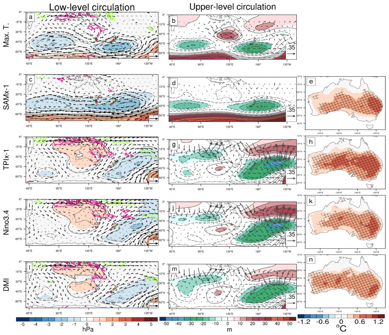
Figure 1Linear regressions of spring standardised weighted area-averaged Australian maximum temperature (a–b), SAMx-1 (c–e), tropical TPIx-1 (f–h), Niño3.4 (i–j), and DMI (j–n) onto low-level circulation (left column) and upper-level circulation (middle column) and Australian maximum temperatures (right column). Low-level circulation is represented by anomalous mean sea level pressure (hPa) (black and filled contours), 850 hPa wind vectors (m s−1), and 500 hPa omega (hPa s−1) contours from −0.02 to 0.02 hPa s−1 in steps of 0.01 hPa s−1 (magenta contours are positive ( downward motion), and cyan contours are negative (upward motion), and the zero contour is not plotted). Upper-level circulation is represented by 200 hPa geopotential height (black and filled contours and wave activity flux vectors (m2 s−2)). Filled contours, bold wind vectors, cross-hatching, and all vertical motion contours are significant at the 95 % confidence level using Student's t test with 39 independent samples.
The tropical modes, represented by Niño3.4 (Fig. 1i–k), the DMI (Fig. 1l–n), and tropical TPI (x−1) (Fig. 1f–h)), are also associated with high spring Australian maximum temperature anomalies. Each mode generates an apparent Rossby wave pattern that arcs from the tropical Indian Ocean to promote anomalous high geopotential height south of Australia, consistent with earlier studies (e.g. Cai et al., 2011; Timbal and Hendon, 2011; McIntosh and Hendon, 2018). The tropical TPI (x−1) is a blend of both Niño3.4 and DMI circulation patterns and has a strong relationship with Australian spring maximum temperatures across all but northern Australia. Each tropical regression also shares anomalous high surface pressure over Australia, sinking motion in the east, cyclonic nodes to the southwest and east of Australia, and elongated upper-level cyclones in the subtropical Indian Ocean. These similarities are likely the result of the strong co-variability between the IOD and ENSO (e.g. Meyers et al., 2007; Risbey et al., 2009a). However, the IOD has a stronger low-level cyclone to the southeast and a poleward extension of the subtropical Indian Ocean cyclone that sets a subtly different wave train from around 50∘ S, 60∘ E that is poleward of that generated by ENSO. The positive IOD is also associated with high maximum temperatures across a broader region of southern and western Australian than El Niño is.
Given the similarities and connections between ENSO and the IOD teleconnections, we use the tropical TPI to represent the large-scale influence of the tropics. The SAM is used to represent the influence of the extratropics. Statistical models of Australian weighted area-averaged spring maximum temperatures reconstructed through multilinear regression using either Niño3.4, DMI, and the SAM or only the tropical TPI and the SAM as the predictors explain similar levels of maximum temperature variability (32 % and 34 % respectively; Fig. S2).
We next compare the atmospheric circulation associated with spring monthly high maximum temperatures to that with the large-scale modes of variability. To ensure that we are assessing the influence of the tropics and extratropics separately, we use multilinear regression onto the monthly circulation variables.
The regression of monthly Australian maximum temperature onto the lower and upper-level atmospheric circulation is displayed in Figs. 2a–c and 3a–c respectively for September, October, and November. The multilinear regression onto the standardised monthly indices of the SAM (x−1) and the tropical TPI (x−1) is in Figs. 2d–j and 3d–j. At first glance, these monthly circulation patterns are similar to the spring-average regression patterns. However, the details of the circulation patterns change as the months progress.

Figure 2Regressions onto low-level circulation, as in Fig. 1, except for September (left column), October (middle column), and November (right column). Standardised area-averaged Australian maximum temperature is linearly regressed onto low-level circulation (a–c), and SAMx-1 (d–f) and tropical TPIx-1 (g–i) are multilinear regressions onto low-level circulation.
Pattern correlation between the maximum temperature MSLP regressions and the SAM and tropical TPI regressions calculated over 5–70∘ S, 70–170∘ E is written in the top right of each SAM or tropical TPI regression.
The boxes (a–c) show key low-level circulation features identified as being important for maximum temperature development: the southwest cyclone (SWC), 35–55∘ S, 70–120∘ E; southeast cyclone (SEC), 45–60∘ S, 160–200∘ E; and Tasman Sea high (TSH), 20–40∘ S, 150–170∘ E.
The most obvious change in atmospheric circulation through the months is in the low-level flow across Australia, particularly generated by the barotropic cyclones southwest (SWC) or southeast (SEC) of Australia (boxes in Fig. 2a–b). Weak anomalous low-level anticyclonic flow around the Tasman Sea (box in Fig. 2c) also contributes to the anomalous northerly flow over eastern Australia in November in particular (Fig. 2c). Tasman Sea anticyclonic blocking patterns have previously been linked to anomalously warm conditions (Marshall et al., 2014) but here appear to only contribute to high maximum temperatures in November. The SWC and SEC vary in geographic shape and strength through the months. The SWC dominates in September but weakens through October and November, whereas the SEC is missing in September but is strong in October and November. Similar cyclones appear in the monthly SAM (x−1) regressions (Figs. 2d–f, 3d–f), and the Australian-region MSLP correlates strongly with that associated with high Australian temperature (top right of Fig. 2d–f). Rather than cyclones in September and October, the TPI (x−1) is associated with a barotropic anticyclone south of Australia that directs anomalous southerly low-level wind across eastern Australia (Figs. 2h–j), a pattern that would be associated with anomalously cooler conditions. The September and October TPI (x−1) MSLP patterns anti-correlate with those associated with high Australian maximum temperatures (top right Fig. 2g–i). It is not until November that we see a barotropic cyclone to the southeast of Australia associated with the TPI (x−1). So, for the majority of spring, negative-TPI-forced low-level atmospheric circulation appears to counter high maximum temperatures, despite the overall positive relationship in spring (Fig. 1h).
The anomalous southern Australian upper anticyclone (SAA) from the spring pattern is also associated with high maximum temperature in each of the individual spring months (Fig. 3a–c), but its location shifts eastward across Australia through spring. The boxed region was chosen to match earlier studies (Gallant and Lewis, 2016; McKay et al., 2021) but best matches the November position, likely contributing to the stronger relationship between heat and SAA in this month (McKay et al., 2021; see also Sect. 6). The anticyclone in later spring appears to form part of a wave train from a cyclone to the northwest of Australia toward the southeast cyclone. While the monthly TPI regressions have anticyclones in September and October (Fig. 3g–h), they are located too far south relative to Australia, as in the spring-average regression. The regressions onto the SAM (x−1) (Fig. 3d–f) have weak anticyclones over western Australia that are not statistically significant. It is not until November that both the SAM and TPI (x−1) (Fig. 3f, i) have an anticyclone over central-east southern Australia. Both the upper-level SAM and TPI (x−1) regressions correlate moderately with the maximum temperature regression in November, and the SAM and TPI (x−1) anticyclones may form part of the same wave train associated with maximum temperatures. However, the SAM and TPI (x−1) anticyclones are weaker and too far east relative to those associated with high maximum temperatures, such that they may not contribute strongly to the SAA formation. We explore this idea further in Sect. 6.

Figure 3As with Fig. 2 but for upper-level circulation. The Australian-region pattern correlation between the maximum temperature Z200 regressions and SAMx-1 and TPIx-1 is in the top right of each figure. Boxed area (a–c) highlights the southern Australian anticyclone (SAA; 30–40∘ S, 120–150∘ E) that is linked with high maximum temperatures.
While the southern Australian anticyclone is not well explained by the SAM or TPI (x−1) through spring, much of the statistically significant 500 hPa vertical motion associated high maximum temperatures (green and magenta contours, Fig. 2a–c) matches that associated with TPI (Fig. 2h–j) and to a lesser extent the SAM (Fig. 2d–f). In September, sinking motion over subtropical Australia and rising motion over the southern coasts are associated with high maximum temperatures. By November, the rising motion has largely vanished, and the sinking motion has shifted to be over eastern Australia. It was expected that the SAA would generate some of the sinking motion associated with high maximum temperature; however, this vertical motion does not correlate strongly with any of the key circulation features examined here (Table S1).
Changes in wave activity flux help explain some of the changes in the broad-scale circulation changes through spring. In September, WAF predominantly diverges from the southwest cyclone toward the southern Australian anticyclone. In October, a component of WAF also diverges from the eastern tropical Indian Ocean region. By November, the tropical component dominates the WAF and forms part of a very different pattern to the previous two months; continuous WAF follows a wave train that appears to propagate from the far southwest Indian Ocean. This wave joins with a wave out of the tropical Indian Ocean, as indicated by the tropical-origin WAF, to then continue through the southern Australian anticyclone. The latter part of this wave train is similar to the IOD teleconnection highlighted by Cai et al. (2011) in spring. The WAF associated with the SAM and TPI (x−1) also diverges from the extratropics toward the respective anticyclones in September and October. While a broad region of low height in the subtropical Indian Ocean is associated with the TPI, it does not appear to generate WAF that diverges into the extratropics. It is not until November that WAF associated with the TPI (x−1), and weakly with the SAM (x−1), appears to diverge directly from the cyclone in the eastern subtropical Indian Ocean, indicating a wave that joins the anticyclone over southeastern Australia.
Overall, the circulation associated with maximum temperature appears to shift from extratropical to tropical forcing as spring progresses. The SAM projects onto the atmospheric circulation associated with maximum temperatures in September, while the TPI projects more strongly later in spring. The change in WAF associated suggests that there may be a weakening barrier between the tropics and extratropics that influences the Rossby wave propagation through spring.
We find qualitatively similar results if we perform the linear regressions using maximum temperature averaged over sub-regions of Australia, for example southwest or southeast Australia (Fig. S3).
We next explore how the subtropical jet (STJ) may be influencing the WAF through the spring months.
The STJ should effectively block direct propagation of Rossby waves from the tropical Indian Ocean into the extratropics (e.g. Simpkins et al., 2014; Li et al., 2014, 2015a, b). However, the gradual decay of the jet through spring (e.g. see Fig. 9, Ceppi and Hartmann, 2013) may reduce its effectiveness as a Rossby wave block (e.g. Wirth, 2020), allowing for more direct propagation into the extratropics by November. The STJ decay coincides with a decrease in the area with total stationary wavenumber (Ks) less than zero over southern Australia (Fig. 4).

Figure 4Total wave number (Ks) calculated for September, October, and November. Vectors are the wave activity flux repeated from Fig. 3.
The wave activity flux vectors from the maximum temperature, TPI, and SAM (x−1) regressions in Fig. 3 are overlaid in Fig. 4 on the monthly climatological Ks associated with the zonal winds. In September, the WAF associated with high maximum temperature indicates waves propagate through a region of low Ks over southwest Australia and are then directed along the STJ waveguide (e.g. Ambrizzi et al., 1995) (i.e. from high to low latitudes). As the jet weakens in October (Fig. 4b), a portion of WAF also diverges from the tropical Indian Ocean to dissipate on the jet's equatorward flank but mostly propagates from west to east along the STJ waveguide. WAF in November (Fig. 4c) is even more distinctive in showing Rossby waves that propagate along the jet waveguide from a region near Africa, upstream of the figure's western edge, with further contributions from the tropical Indian Ocean.
The increase in WAF out of the tropical Indian Ocean associated with the tropical TPI (Fig. 4h–j) coincides with the STJ decay. In September and October weak WAF diverging from the central southern Indian Ocean indicates wave trains follow the eddy-driven jet waveguide (region of locally higher wave number around 50∘ S). McIntosh and Hendon (2018) proposed that transient eddy feedbacks generate a secondary wave source in winter poleward of the STJ in response to IOD forcing. The high-latitude wave train found in association with the TPI may indicate that this secondary wave source is also important in early spring. The tendency for TPI-associated WAF to follow this trajectory may explain why the barotropic anticyclone associated with the TPI is further poleward than in the regression onto Australian maximum temperature. By October, increased WAF diverges from the tropical Indian Ocean to divert along the region of high Ks. By November, WAF diverges out of the extratropical Indian Ocean along the high Ks region, similar to the maximum temperature-WAF. This increase in tropical-origin WAF is consistent with increased wave trains propagating out of the tropical Indian Ocean associated with the TPI. WAF generated by the SAM (Fig. 4d–f) also converges toward the STJ waveguide in each month.
The STJ acts as a waveguide (Hoskins and Ambrizzi, 1993), with the majority of WAF associated with Australian maximum temperature, and with the tropics and extratropics indicating wave trains divert to propagate along the jet. Limits around linear Rossby wave theory (e.g. Liu and Alexander, 2007) may explain why some wave activity flux crosses the region of imaginary wavenumber associated with the STJ. While the breakdown of the STJ through spring may help explain the change in teleconnection pathways of the TPI toward Australia, it may not directly explain the change in atmospheric circulation associated with maximum temperature.
We now look more closely into how the drivers, circulation features, and heating mechanisms relate to each other and how that results in higher Australian maximum temperatures.
As with the atmospheric circulation regressions, the relationships between Australian maximum temperature and the SAM and TPI (x−1) evolve through the spring months. In September, the negative phase of the SAM (Fig. 5a) is associated with a broad area of high maximum temperature over subtropical Australia, that contracts in October and November (Figs. 5b–c). Conversely, the relationship with the negative TPI and maximum temperature is weaker early in spring, with statistically significant high temperatures confined to the west and east and cool temperatures in the far north in September (Fig. 5d). The TPI's relationship with high maximum temperature broadens and strengthens in October and covers the majority of Australia by November (Figs. 5e–f). Overall, these monthly relationships give the impression of a transition from extratropical to tropical drivers becoming more influential over Australian temperatures that is broadly consistent with the apparent change in atmospheric circulation through spring.
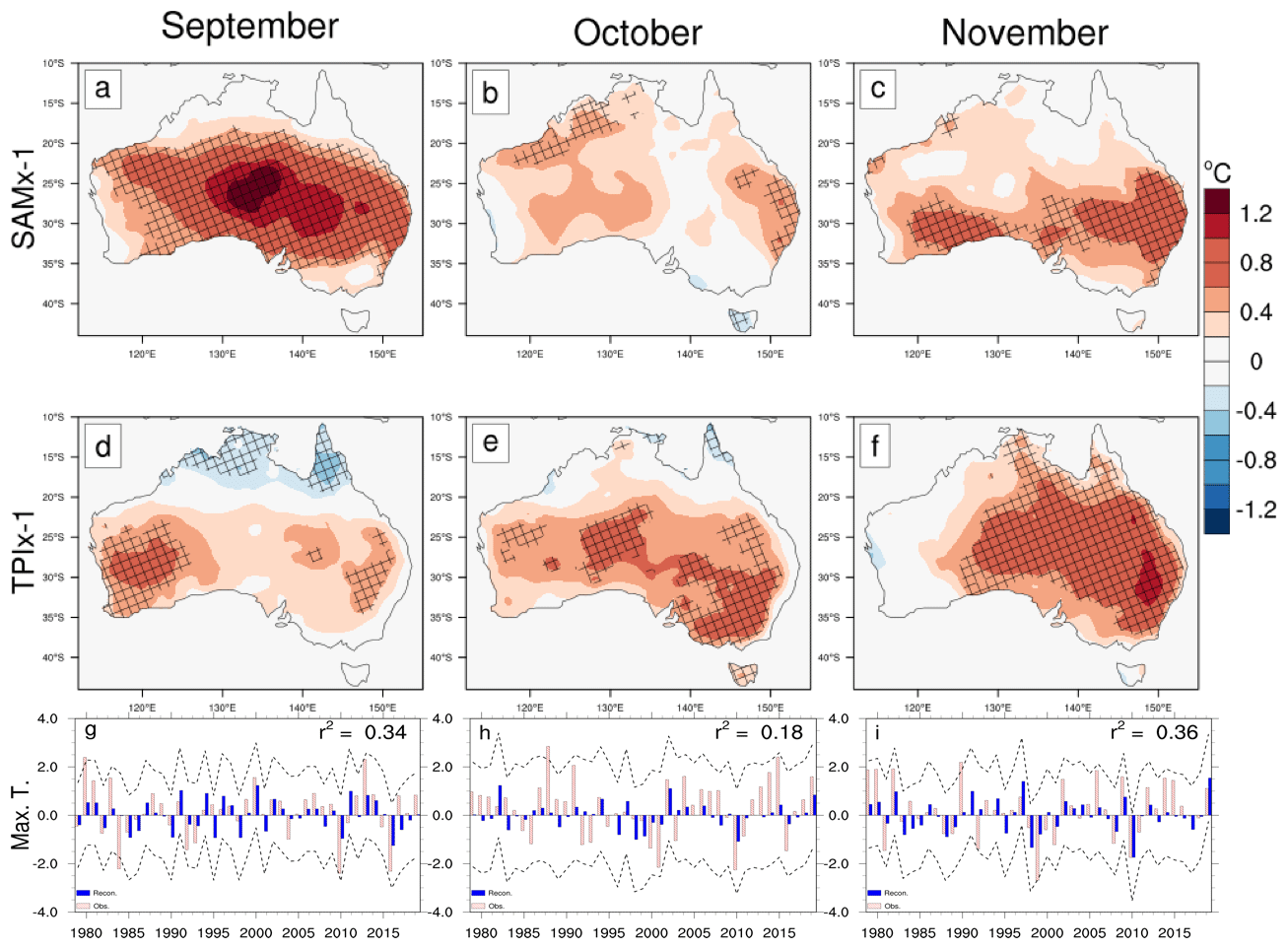
Figure 5Multilinear regression coefficients (∘C) of Australian maximum temperature regressed onto standardised time series of the SAMx-1 (a–c) and the tropical TPIx-1 (d–f) for September, October, and November over the years 1979 to 2019. Reconstructions (blue bars) of September, October, and November (g–i) Australian-area-averaged maximum temperature from standardised time series of the SAM and tropical TPI indices. Observed values are shown as red bars. The dashed line shows the 95 % prediction interval computed as ±1.96 standard error, and the variance explained (r2) by the model is in the top right of each panel.
Using the standardised SAM and TPI time series as predictors in a regression model to reconstruct the monthly Australian-averaged maximum temperature anomalies (Fig. 4g–i) explains only between 18 % and 36 % Australian maximum temperature variance (r2) through spring. The model does not substantially improve if it is calculated over southeast or southwest Australia or if using Niño3.4 or DMI as predictors instead of the tropical TPI (Fig. S4).
To explore how the atmospheric circulation relates to some of the mechanisms that develop heat through spring, we first compose indices of the key circulation features discussed in Sect. 4. The three circulation-feature indices are mean sea level pressure (multiplied by −1) weighted area averages over the southwest and southeast cyclones (SWC and SEC) and 200 hPa geopotential height over the southern Australian anticyclone (SAA) for each spring month. See Figs. 2a and b and 3a–c for regions. Creating a statistical model of Australian-averaged monthly spring maximum temperatures from these circulation features (Fig. 6a–c) explains consistently higher maximum temperature variance (around 60 %) than the model from the indices of tropical and extratropical large-scale modes of variability did. Further, despite the changes in the features' geographic shape, strength, and position across the spring months in Fig. 2, the majority of maximum temperature across Australia is well explained by at least one of these features at all times through spring (Fig. S5). We next explore how these MSLP or 200 hPa geopotential height features relate to the anomalous low-level westerly or northerly winds and vertical motion and how that relates to high maximum temperature development.
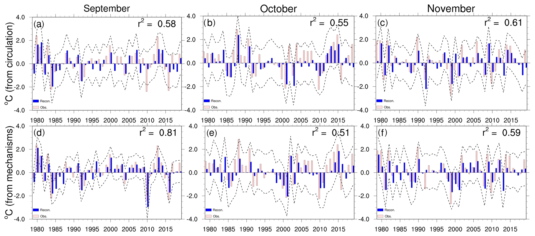
Figure 6As in Fig. 4g–i but using time series of key circulation features (southwest low, southeast low, and southern Australian anticyclone) identified in Figs. 1 and 2 as predictors in the top row (a–c) and area-averaged dynamical heat mechanism components (850 hPa zonal wind and meridional wind (multiplied by −1) and 500 hPa vertical motion; see text for region averaged over) as predictors in the bottom row (d–e) for September, October, and November.
Following van Rensch et al. (2019), indices of three dynamical heating mechanisms were created by weighted area-averaging of westerly and northerly wind (meridional wind multiplied by −1) anomalies over a region around southern Australia (25–45∘ S, 105–155∘ E) and 500 hPa vertical motion anomalies (omega; positive is sinking motion) averaged over subtropical Australia (15–25∘ S, 120–155∘ E). Regions were selected based on the areas of highest statistical significance between atmospheric circulation and Australian maximum temperature in Fig. 2a–c. A statistical model of Australian-averaged maximum temperatures that uses these mechanisms as the predictors explains a higher proportion of maximum temperature variance through spring than the model using the SAM or tropical TPI does (Fig. 6d–e). The percent variance explained is higher in September (about 80 %), before dropping to around 55 % in October–November. This decrease appears to be primarily associated with how strongly the anomalous westerly winds correlate with maximum temperature over southern Australia; a strong positive relationship with anomalous westerly wind in September changes to insignificant or negative in October and November (Fig. S6a–c). There is also an increase in negative correlation between maximum temperatures and anomalous northerly winds in northeastern Australia (Fig. S6d–e) that will partly offset the increasing positive relationship further poleward. These changing relationships between dynamical mechanisms and maximum temperature through spring are linked with the changing relationships with the circulation features (Table S1). Overall, the three dynamical heating mechanisms explain much of Australia's monthly spring maximum temperature variability.
Figure 7 summarises the relationship between Australian maximum temperatures, circulation features, dynamical heating mechanisms, and climate drivers through the spring months. The correlation between the SEC and Australian maximum temperature is strongest in September and rapidly decreases through October and November, and simultaneously the correlations with the SWC and particularly the SAA increase. As expected from Fig. 2, the SEC and SWC are more closely linked with the extratropics. Linearly regressing out the SAM component from time series of the SWC and SEC reduces the correlation strength with Australian maximum temperature (Fig. 7a), particularly in September. Conversely, linearly removing the tropical TPI slightly increases the correlation between the cyclones and temperature, with the partial-correlation only weakening in November. As the SAM is strongly related to the barotropic cyclones it is also strongly related to how temperature changes with the anomalous westerly wind. Linearly removing the SAM from the westerly wind time series nearly halves the correlation with maximum temperature in September and weakens the correlation in October and November (Fig. 7b). Conversely, linearly removing the tropical TPI actually slightly increases the correlation with the westerly wind anomalies in September and October but decreases the correlation in November.
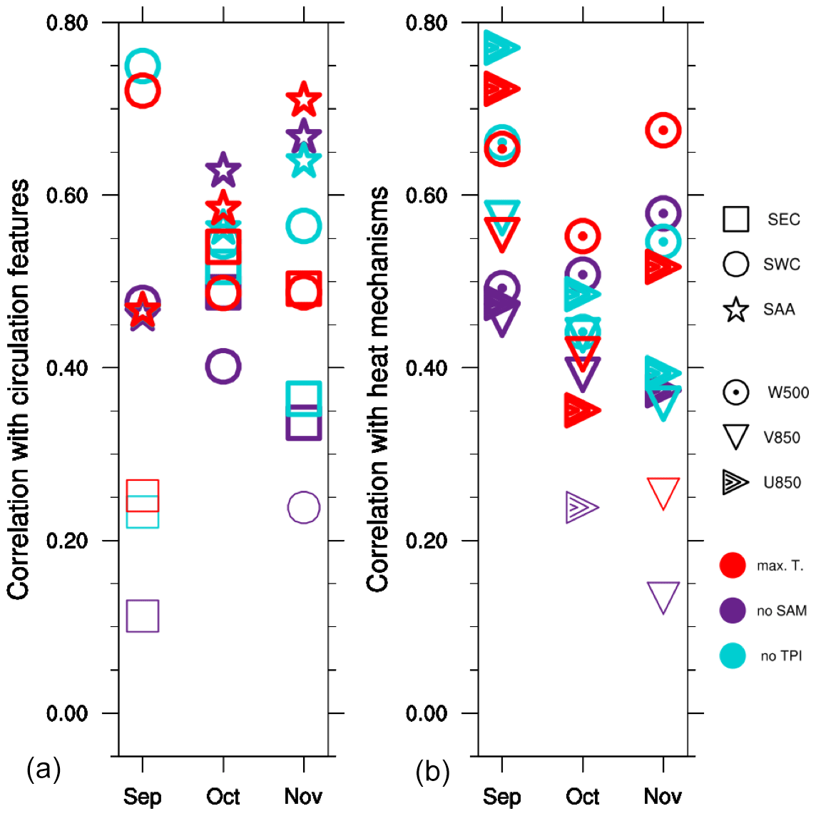
Figure 7Correlations between Australian area-averaged maximum temperature (red) between key atmospheric circulation features (a) and dynamical heating mechanisms (b) for September, October, and November. The purple and turquoise show partial correlations of the same but with the SAM and tropical TPI linearly removed. Bold lines show the correlation was statistically significant at the 95 % confidence level using Student's t test with 39 samples.
The relationships with anomalous northerly wind and sinking motion and Australian-averaged maximum temperature do not change as dramatically with the removal of the SAM or TPI. Anomalous northerly wind is not strongly influenced by the tropics or extratropics in September or October, but the correlation strengthens and weakens in November with the removal of the TPI and the SAM, respectively. While removing the SAM and TPI from the SAA had relatively little influence on the correlation with Australian maximum temperatures, removing the SAM from sinking motion in September and both the TPI and the SAM in October and November reduced the correlation. Overall, it appears that the heating mechanisms associated with high maximum temperatures in spring are subject to the changing influence of the extratropics and tropics on the local atmospheric circulation features through spring.
The sources of the atmospheric circulation patterns associated with high monthly maximum temperatures in Australia appear to change from primarily extratropical in early spring to tropical in late spring. Examination of three dynamical heating mechanisms (anomalous low-level winds broken into westerly and northerly components, and anomalous mid-tropospheric sinking motion) indicates that this shift may be due to a change in how heat develops. In early spring, the low-level wind plays a greater role in maximum temperatures, advecting relatively warmer air from the subtropical oceans over the cold landmass. We argue that this wind correlates strongly with the extratropics, as the SAM projects strongly onto the southwest and southeast cyclones that direct a lot of the low-level flow around Australia. Conversely, the atmospheric circulation associated with the TPI (x−1) acts to counter the low-level flow that drives higher temperatures. Thus, in early spring we have a closer association with heat production and the extratropics. By late spring, the circulation patterns associated with high temperature have changed, and the wind does not correlate as strongly with temperature. As such, adiabatic sinking over subtropical Australia has a proportionally stronger correlation with high temperatures. Both the SAM and TPI (x−1) regressions show sinking motion in the subtropics through spring. El Niño can promote the negative phase of the SAM from late spring (L'Heureux and Thompson, 2006; Hendon et al., 2007; Lim et al., 2016; Lim et al., 2019a). However, it is the TPI not the SAM that better matches the sinking motion over eastern Australia in November. Hence, the apparent change from extratropical to tropical forcing in the circulation pattern is likely because the tropics promote more of the heat developing mechanisms later in spring. However, much of the atmospheric patterns associated with heat through spring are explained by neither the tropical TPI nor the SAM.
The subtropical jet appears to play a greater role in Australian spring heat by acting as a wave guide (Hoskins and Ambrizzi, 1993) that directs quasi-stationary Rossby waves toward Australia, rather than as a block that limits direct propagation of Rossby waves from the tropical Indian Ocean to the Southern Hemisphere extratropics (e.g. Simpkins et al., 2014; Li et al., 2015a, b). Wave activity flux appears to indicate wave propagation occurs directly out of the tropical Indian Ocean later in spring. However, the upper-level atmospheric anomalies through spring are broadly consistent with IOD-forced wave trains identified in the literature, with shifts poleward or equatorward as discussed above (Cai et al., 2011; McIntosh and Hendon, 2018; Wang et al., 2019). As such, the secondary wave source in the high latitudes of the Indian Ocean proposed by McIntosh and Hendon (2018) may be key for promoting the TPI-forced atmospheric circulation in early spring. Overall, the STJ decay appears to be a lesser factor than the dynamical heating mechanisms in the apparent change from extratropical to tropical forcing of maximum temperatures through spring. To test this idea, wave activity flux is calculated from regressions of the three dynamical heating mechanisms onto 200Z (Fig. S7). As spring progresses, WAF associated with the heating mechanisms indicates greater Rossby wave propagation out of the tropics than the extratropics. Waves appear to propagate along the jet waveguide toward Australia, reflecting the growing relationship between the tropics and temperature.
Area-averaged anomalous low-level wind and vertical motion were used to understand how the atmospheric circulation relates to Australia-wide maximum temperatures and explain much of the spring maximum temperature variability. However, it was not always clear how the atmospheric circulation features influenced those heating mechanisms. The southern Australian anticyclone and 500 hPa subtropical-Australian sinking motion, while important for heat, appear to be largely uncorrelated with the other circulation features and mechanisms. Greater insight into how remote forcing of the atmospheric circulation results in high Australian temperatures could be gained by including other heating mechanisms in future analyses, including insolation (Lim et al., 2019b), changes to synoptic weather systems (Cai et al., 2011; Hauser et al., 2020), and land-surface feedbacks linked to antecedent moisture (e.g. Seneviratne et al., 2010; Arblaster et al., 2014; Hirsch and King, 2020). Including the preceding month's Australian-averaged rainfall anomaly as an additional predictor of Australian monthly maximum temperatures did increase the percent variance explained by the statistical model (Fig. S8) but only in later spring. Dry conditions have been noted as an important factor in Australian summer heatwaves (Hirsch et al., 2019; Loughran et al., 2019; Hirsch and King, 2020) and may be important for extreme heat in late spring.
While simplifying heating mechanisms into three separate indices was useful, geographic differences across Australia and interactions between mechanisms should also be considered. The combination of poleward advection of adiabatically warmed air after it descends anticyclonically over the Tasman Sea has been identified as a key mechanism for summer heatwaves in southeast Australia (e.g. Quinting and Reeder, 2017). This combination of mechanisms may generate heat through spring, particularly in the east and in November. The rising motion over southern Australia requires further investigation as it may be another factor in the combination of heat mechanisms. Air diabatically warmed in association with storminess just to Australia's south may then be advected and descend toward Australia.
We used the tropical TPI to represent tropical variability relevant to Australia's maximum temperature, but other indices or drivers may highlight different Rossby wave pathways or heating mechanisms. Reconstructing Australian maximum temperature time series with more commonly used indices for the IOD and ENSO did not change the effectiveness of the statistical models overall (Fig. S4). However, this model did show a stronger relationship between temperature and the IOD in early spring and ENSO in later spring, consistent with earlier studies (Jones and Trewin, 2000; Saji et al., 2005). As such, monthly IOD regressions onto atmospheric circulation may produce different wave trains earlier in spring than found with the tropical TPI. The MJO may also influence the atmospheric circulation associated with monthly maximum temperature development. MJO-initiated Rossby wave trains from the western Pacific promote low winter minimum temperatures in Australia (Wang and Hendon, 2020) and from the tropical Indian Ocean promote high spring maximum temperatures in Australia (Wang and Hendon, personal communication, 2021). The positive phase of the IOD suppresses MJO activity across the Indian Ocean (Wilson et al., 2013), possibly restricting the MJO's influence on Australia's maximum temperature. However, MJO activity in the tropical Indian Ocean has recently been found to counter the wetting influence of La Niña during spring (Lim et al., 2021b). As such the MJO may be an important factor for spring maximum temperatures, particularly when the tropical SSTs are not otherwise conducive for high temperatures.
As the trend toward higher Australian spring temperatures is projected to continue into the future, a better understanding of what drives maximum temperatures over the months of spring is critical. A combination of extreme values in remote tropical and extratropical drivers of variability exacerbated already dry and hot conditions in spring 2019 to promote one of Australia's deadliest fire seasons (Watterson, 2020; Lim et al., 2021a; Abram et al., 2021; Marshall et al., 2022). Further, projected trends toward positive IOD (Cai et al., 2014; Abram et al., 2020) may contribute to higher maximum temperatures in the future, particularly in later spring when the tropics exert greater influence on Australia's dynamical heating mechanisms. As we have shown just how different the atmospheric circulation and heating mechanisms can be through a season in Australia, other regions and seasons could also benefit from similar analysis, particular as the world continues to warm (e.g. Collins et al., 2013).
The code for analysis is available from the corresponding author on request. ERA5-reanalysis data are available from Copernicus Climate Change Service at https://www.ecmwf.int/en/forecasts/datasets/reanalysis-datasets/era5 (last access: 14 January 2022; ECMWF, 2022). AWAP data are available from the Australian Bureau of Meteorology. ERSSTv5 SST data is available for download from NOAA at https://www.ncei.noaa.gov/products/extended-reconstructed-sst (last access: 6 July 2020; NOAA, 2020).
The supplement related to this article is available online at: https://doi.org/10.5194/wcd-3-413-2022-supplement.
RCM produced the figures and wrote the initial draft manuscript. All authors contributed to analysis and editing of the manuscript.
The contact author has declared that neither they nor their co-authors have any competing interests.
Publisher’s note: Copernicus Publications remains neutral with regard to jurisdictional claims in published maps and institutional affiliations.
This research was undertaken at the NCI National Facility in Canberra, Australia, which is supported by the Australian Commonwealth Government. The NCAR Command Language (NCL; http://www.ncl.ucar.edu, last access: 14 January 2022) version 6.4.0 was used for data analysis and visualisation of the results. We thank Guomin Wang for his assistance writing code for analysis and Zoe Gillett, Eun-Pa Lim, and Harry Hendon for their insights into the data. The authors thank Thea Turkington for supplying the tropical tripole index dataset. We thank Harry Hendon and Andrew Marshall for their constructive feedback on an earlier version of the manuscript. We thank two anonymous reviewers for the insightful and helpful comments.
Roseanna C. McKay and Julie M. Arblaster were supported by the Australian Research Council (ARC) Centre of Excellence for Climate Extremes (grant no. CE170100023). Roseanna C. McKay was also supported by an Australian Government Research Training Program (RTP) Scholarship and a Bureau of Meteorology PhD Top-up scholarship. Julie M. Arblaster received partial funding from the Regional and Global Model Analysis component of the Earth and Environmental System Modeling Program of the US Department of Energy’s Office of Biological & Environmental Research via the National Science Foundation (grant no. IA 1947282). Pandora Hope received funding from the Climate Systems Hub of the Australian Government’s National Environmental Science Program (NESP).
This paper was edited by Daniela Domeisen and reviewed by Andrea Taschetto and one anonymous referee.
Abram, N. J., Wright, N. M., Ellis, B., Dixon, B. C., Wurtzel, J. B., England, M. H., Ummenhofer, C. C., Philibosian, B., Cahyarini, S. Y., Yu, T.-L., Shen, C.-C., Cheng, H., Edwards, R. L., and Heslop, D.: Coupling of Indo-Pacific climate variability over the last millennium, Nature, 579, 385–392, https://doi.org/10.1038/s41586-020-2084-4, 2020.
Abram, N. J., Henley, B. J., Sen Gupta, A., Lippmann, T. J. R., Clarke, H., Dowdy, A. J., Sharples, J. J., Nolan, R. H., Zhang, T., Wooster, M. J., Wurtzel, J. B., Meissner, K. J., Pitman, A. J., Ukkola, A. M., Murphy, B. P., Tapper, N. J., and Boer, M. M.: Connections of climate change and variability to large and extreme forest fires in southeast Australia, Commun. Earth Environ., 2, 8, https://doi.org/10.1038/s43247-020-00065-8, 2021.
Ambrizzi, T., Hoskins, B. J., and Hsu, H.-H.: Rossby wave propagation and teleconnection patterns in austral winter, J. Atmos. Sci., 52, 3661–3672, https://doi.org/10.1175/1520-0469(1995)052<3661:RWPATP>2.0.CO;2, 1995.
Arblaster, J., Lim, E.-P., Hendon, H., Trewin, B., Wheeler, M., Liu, G., and Braganza, K.: UNDERSTANDING AUSTRALIA'S HOTTEST SEPTEMBER ON RECORD, B. Am. Meteorol. Soc., 95, S37–S41, 2014.
Bals-Elsholz, T. M., Atallah, E. H., Bosart, L. F., Wasula, T. A., Cempa, M. J., and Lupo, A. R.: The Wintertime Southern Hemisphere Split Jet: Structure, Variability, and Evolution, J. Climate, 14, 4191–4215, 2001.
Barnes, E. A. and Hartmann, D. L.: Detection of Rossby wave breaking and its response to shifts of the midlatitude jet with climate change: WAVE BREAKING AND CLIMATE CHANGE, J. Geophys. Res.-Atmos., 117, D09117, https://doi.org/10.1029/2012JD017469, 2012.
Boschat, G., Pezza, A., Simmonds, I., Perkins, S., Cowan, T., and Purich, A.: Large scale and sub-regional connections in the lead up to summer heat wave and extreme rainfall events in eastern Australia, Clim. Dynam., 44, 1823–1840, https://doi.org/10.1007/s00382-014-2214-5, 2015.
Cai, W., van Rensch, P., Cowan T., and Hendon H. H.: Teleconnection Pathways of ENSO and the IOD and the Mechanisms for Impacts on Australian Rainfall, J. Climate, 24, 3910–3923, https://doi.org/10.1175/2011JCLI4129.1, 2011.
Cai, W., Santoso, A., Wang, G., Weller, E., Wu, L., Ashok, K., Masumoto, Y., and Yamagata, T.: Increased frequency of extreme Indian Ocean Dipole events due to greenhouse warming, Nature, 510, 254–258, https://doi.org/10.1038/nature13327, 2014.
Ceppi, P., and Hartmann, D. L.: On the Speed of the Eddy-Driven Jet and the Width of the Hadley Cell in the Southern Hemisphere, J. Climate, 26, 3450–3465, https://doi.org/10.1175/JCLI-D-12-00414.1, 2013.
Collins, M., Knutti, R., Arblaster, J., Dufresne, J.-L., Fichefet, T., Friedlingstein, P., Gao, X., Gutowski, W. J., Johns, T., Krinner, G., Shongwe, M., Tebaldi, C., Weaver, A. J., Wehner, M. F., Allen, M. R., Andrews, T., Beyerle, U., Bitz, C. M., Bony, S., and Booth, B. B. B.: Long-term Climate Change: Projections, Commitments and Irreversibility, Climate Change 2013 – The Physical Science Basis: Contribution of Working Group I to the Fifth Assessment Report of the Intergovernmental Panel on Climate Change, 1029–1136, 2013.
Cullen, B. R., Johnson, I. R., Eckard, R. J., Lodge, G. M., Walker, R. G., Rawnsley, R. P., and McCaskill, M. R.: Climate change effects on pasture systems in south-eastern Australia, Crop Pasture Sci., 60, 933, https://doi.org/10.1071/CP09019, 2009.
Dee, D. P., Uppala, S. M., Simmons, A. J., Berrisford, P., Poli, P., Kobayashi, S., Andrae, U., Balmaseda, M. A., Balsamo, G., Bauer, P., Bechtold, P., Beljaars, A. C. M., van de Berg, L., Bidlot, J., Bormann, N., Delsol, C., Dragani, R., Fuentes, M., Geer, A. J., and Vitart, F.: The ERA-Interim reanalysis: Configuration and performance of the data assimilation system, Q. J. Roy. Meteorol. Soc., 137, 553–597, https://doi.org/10.1002/qj.828, 2011.
Dowdy, A. J.: Climatological Variability of Fire Weather in Australia, J. Appl. Meteorol. Climatol., 57, 221–234, https://doi.org/10.1175/JAMC-D-17-0167.1, 2018.
ECMWF: ERA5, ECMWF [data set], https://www.ecmwf.int/en/forecasts/datasets/reanalysis-datasets/era5, last access: 14 January 2022.
Fischer, E. M., Seneviratne, S. I., Lüthi, D., and Schär, C.: Contribution of land-atmosphere coupling to recent European summer heat waves, Geophys. Res. Lett., 34, L06707, https://doi.org/10.1029/2006GL029068, 2007.
Fogt, R. L. and Marshall, G. J.: The Southern Annular Mode: Variability, trends, and climate impacts across the Southern Hemisphere, WIREs Climate Change, 11, e652, https://doi.org/10.1002/wcc.652, 2020.
Gallant, A. J. E. and Lewis, S. C.: Stochastic and anthropogenic influences on repeated record-breaking temperature extremes in Australian spring of 2013 and 2014: CAUSES OF REPEATED TEMPERATURE RECORDS, Geophys. Res. Lett., 43, 2182–2191, https://doi.org/10.1002/2016GL067740, 2016.
Gibson, P. B., Pitman, A. J., Lorenz, R., and Perkins-Kirkpatrick, S. E.: The Role of Circulation and Land Surface Conditions in Current and Future Australian Heat Waves, J. Climate, 30, 9933–9948, https://doi.org/10.1175/JCLI-D-17-0265.1, 2017.
Gillett, Z. E., Hendon, H. H., Arblaster, J. M., and Lim, E.-P.: Tropical and Extratropical Influences on the Variability of the Southern Hemisphere Wintertime Subtropical Jet, J. Climate, 34, 4009–4022, https://doi.org/10.1175/JCLI-D-20-0460.1, 2021.
Gong, D. and Wang, S.: Definition of Antarctic Oscillation index, Geophys. Res. Lett., 26, 459–462, https://doi.org/10.1029/1999GL900003, 1999.
Harris, S., and Lucas, C.: Understanding the variability of Australian fire weather between 1973 and 2017, PLoS ONE, 14, e0222328, https://doi.org/10.1371/journal.pone.0222328, 2019.
Hauser, S., Grams, C. M., Reeder, M. J., McGregor, S., Fink, A. H., and Quinting, J. F.: A weather system perspective on winter–spring rainfall variability in southeastern Australia during El Niño, Q. J. Roy. Meteorol. Soc., 146, 2614–2633, https://doi.org/10.1002/qj.3808, 2020.
Hendon, H. H., Thompson, D. W. J., and Wheeler, M. C.: Australian Rainfall and Surface Temperature Variations Associated with the Southern Hemisphere Annular Mode, J. Climate, 20, 2452–2467, https://doi.org/10.1175/JCLI4134.1, 2007.
Hendon, H. H., Lim, E.-P., and Nguyen, H.: Seasonal Variations of Subtropical Precipitation Associated with the Southern Annular Mode, J. Climate, 27, 3446–3460, https://doi.org/10.1175/JCLI-D-13-00550.1, 2014.
Hersbach, H., Bell, B., Berrisford, P., Hirahara, S., Horányi, A., Muñoz-Sabater, J., Nicolas, J., Peubey, C., Radu, R., Schepers, D., Simmons, A., Soci, C., Abdalla, S., Abellan, X., Balsamo, G., Bechtold, P., Biavati, G., Bidlot, J., Bonavita, M., and Thépaut, J.: The ERA5 global reanalysis, Q. J. Roy. Meteorol. Soc., 146, 1999–2049, https://doi.org/10.1002/qj.3803, 2020.
Hirsch, A. L. and King, M. J.: Atmospheric and Land Surface Contributions to Heatwaves: An Australian Perspective, J. Geophys. Res.-Atmos., 125, https://doi.org/10.1029/2020JD033223, 2020.
Hirsch, A. L., Evans, J. P., Di Virgilio, G., Perkins-Kirkpatrick, S. E., Argüeso, D., Pitman, A. J., Carouge, C. C., Kala, J., Andrys, J., Petrelli, P., and Rockel, B.: Amplification of Australian Heatwaves via Local Land-Atmosphere Coupling, J. Geophys. Res.-Atmos., 124, 13625–13647, https://doi.org/10.1029/2019JD030665, 2019.
Hope, P. and Watterson, I.: Persistence of cool conditions after heavy rain in Australia, J. Southern Hemisphere Earth Syst. Sci., 68, 41–64, https://doi.org/10.22499/3.6801.004, 2018.
Hope, P., Lim, E.-P., Wang, G., Hendon, H. H., and Arblaster, J. M.: Contributors to the Record High Temperatures Across Australia in Late Spring 2014, B. Am. Meteorol. Soc., 96, S149–S153, 2015.
Hope, P., Wang, G., Lim, E.-P., Hendon, H. H., and Arblaster, J. M.: WHAT CAUSED THE RECORD-BREAKING HEAT ACROSS AUSTRALIA IN OCTOBER 2015?, in: Explaining Extreme Events of 2015 from a Climate Perspective, B. Am. Meteorol. Soc., 96, S1–S172, https://doi.org/10.1175/BAMS-D-15-00157.1, 2016.
Hoskins, B. J. and Karoly, D. J.: The Steady Linear Response of a Spherical Atmosphere to Thermal and Orographic Forcing, J. Atmos. Sci., 38, 1179–1196, https://doi.org/10.1175/1520-0469(1981)038<1179:TSLROA>2.0.CO;2, 1981.
Hoskins, B. J. and Ambrizzi, T.: Rossby wave propagation on a realistic longitudinally varying flow, J. Atmos. Sci., 50, 1661–1671, 1993.
Huang, B., Peter, W., Thorne, P. W., Banzon, V. F., Boyer, T., Chepurin, G., Lawrimore, J. H., Menne, M. J., Smith, T. M., Vose, R. S., and Zhang, H.: Extended Reconstructed Sea Surface Temperature version 5 (ERSSTv5), Upgrades, validations, and intercomparisons, J. Climate, 30, 8179–8205, https://doi.org/10.1175/JCLI-D-16-0836.1, 2017.
Hurrell, J., Meehl, G. A., Bader, D., Delworth, T. L., Kirtman, B., and Wielicki, B.: A Unified Modeling Approach to Climate System Prediction, B. Am. Meteorol. Soc., 90, 1819–1832, https://doi.org/10.1175/2009BAMS2752.1, 2009.
Japan Meteorological Agency/Japan, JRA-55: Japanese 55-year Reanalysis, Daily 3-Hourly and 6-Hourly Data, Research Data Archive at the National Center for Atmospheric Research, Computational and Information Systems Laboratory, Boulder, Colo., (Updated monthly), https://doi.org/10.5065/D6HH6H41, 2013.
Jarvis, C., Darbyshire, R., Goodwin, I., Barlow, E. W. R., and Eckard, R.: Advancement of winegrape maturity continuing for winegrowing regions in Australia with variable evidence of compression of the harvest period: Advancement of winegrape maturity, Aust. J. Grape Wine Res., 25, 101–108, https://doi.org/10.1111/ajgw.12373, 2019.
Jones, D. and Trewin, B. C.: On the relationships between the El Niño-Southern Oscillation and Australian land surface temperature, Int. J. Climatol., 23, 697–719, 2000.
Jones, D., Wang, W., and Fawcett, R.: High-quality spatial climate data-sets for Australia, Aust. Meteorol. Oceanogr. J., 58, 233–248, https://doi.org/10.22499/2.5804.003, 2009.
Koch, P., Wernli, H., and Davies, H. C.: An event-based jet-stream climatology and typology, Int. J. Climatol., 26, 283–301, https://doi.org/10.1002/joc.1255, 2006.
L'Heureux, M. L. and Thompson, D. W. J.: Observed Relationships between the El Niño–Southern Oscillation and the Extratropical Zonal-Mean Circulation, J. Climate, 19, 276–287, https://doi.org/10.1175/JCLI3617.1, 2006.
Li, X., Holland, D. M., Gerber, E. P., and Yoo, C.: Impacts of the north and tropical Atlantic Ocean on the Antarctic Peninsula and sea ice, Nature 505, 538–542, https://doi.org/10.1038/nature12945, 2014.
Li, X., Gerber, E. P., Holland, D. M., and Yoo, C.: A Rossby Wave Bridge from the Tropical Atlantic to West Antarctica, J. Climate, 28, 2256–2273, https://doi.org/10.1175/JCLI-D-14-00450.1, 2015a.
Li, X., Holland, D. M., Gerber, E. P., and Yoo, C.: Rossby Waves Mediate Impacts of Tropical Oceans on West Antarctic Atmospheric Circulation in Austral Winter, J. Climate, 28, 8151–8164, https://doi.org/10.1175/JCLI-D-15-0113.1, 2015b.
Lim, E. P., Hendon, H. H., Arblaster, J. M., Chung, C., Moise, A. F., Hope, P., Young, G., and Zhao, M.: Interaction of the recent 50 year SST trend and La Niña 2010: amplification of the Southern Annular Mode and Australian springtime rainfall, Clim. Dynam., 47, 2273–2291, https://doi.org/10.1007/s00382-015-2963-9, 2016.
Lim, E.-P., Hendon, H., Hope, P., Chung, C., Delage, F., and McPhaden, M. J.: Continuation of tropical Pacific Ocean temperature trend may weaken extreme El Niño and its linkage to the Southern Annular Mode, Sci. Rep., 15, 17044, https://doi.org/10.1038/s41598-019-53371-3, 2019a.
Lim, E.-P., Hendon, H. H., Boschat, G., Hudson, D., Thompson, D. W. J., Dowdy, A. J., and Arblaster, J. M.: Australian hot and dry extremes induced by weakenings of the stratospheric polar vortex, Nat. Geosci., 12, 896–901, https://doi.org/10.1038/s41561-019-0456-x, 2019b.
Lim, E.-P., Hendon, H. H., Butler, A. H., Thompson, D. W. J., Lawrence, Z. D., Scaife, A. A., Shepherd, T. G., Polichtchouk, I., Nakamura, H., Kobayashi, C., Comer, R., Coy, L., Dowdy, A., Garreaud, R. D., Newman, P. A., and Wang, G.: The 2019 Southern Hemisphere Stratospheric Polar Vortex Weakening and Its Impacts, B. Am. Meteorol. Soc., 102, E1150–E1171, https://doi.org/10.1175/BAMS-D-20-0112.1, 2021a.
Lim, E.-P., Hudson, D., Wheeler, M. C., Marshall, A. G., King, A., Zhu, H., Hendon, H. H., de Burgh-Day, C., Trewin, B., Griffiths, M., Ramchurn, A., and Young, G.: Why Australia was not wet during spring 2020 despite La Niña, Sci. Rep., 11, 18423, https://doi.org/10.1038/s41598-021-97690-w, 2021b.
Liu, Z. and Alexander, M.: Atmospheric bridge, oceanic tunnel, and global climatic teleconnections, Rev. Geophys., 45, RG2005, https://doi.org/10.1029/2005RG000172, 2007.
Loughran, T. F., Pitman, A. J., and Perkins-Kirkpatrick, S. E.: The El Niño-Southern Oscillation’s effect on summer heatwave development mechanisms in Australia, Clim. Dynam., 52, 6279–6300, https://doi.org/10.1007/s00382-018-4511-x, 2019.
Marshall, A., Hudson, D., Wheeler, M., Alves, O., Hendon, H., Pook, M., and Risbey, J.: Intra-seasonal drivers of extreme heat over Australia in observations and POAMA-2, Clim. Dynam., 43, 1915–1937, https://doi.org/10.1007/s00382-013-2016-1, 2014.
Marshall, A. G., Hudson, D., Wheeler, M. C., Hendon, H. H., and Alves, O.: Simulation and prediction of the Southern Annular Mode and its influence on Australian intra-seasonal climate in POAMA, Clim. Dynam., 38, 2483–2502, https://doi.org/10.1007/s00382-011-1140-z, 2012.
Marshall, A. G., Gregory, P. A., de Burgh-Day, C. O., and Griffiths, M.: Subseasonal drivers of extreme fire weather in Australia and its prediction in ACCESS-S1 during spring and summer, Clim. Dynam., 58, 523–553, https://doi.org/10.1007/s00382-021-05920-8, 2022.
McIntosh, P. C. and Hendon, H. H.: Understanding Rossby wave trains forced by the Indian Ocean Dipole, Clim. Dynam., 50, 2783–2798, https://doi.org/10.1007/s00382-017-3771-1, 2018.
McKay, R. C., Arblaster, J. M., Hope, P., and Lim, E.-P.: Exploring atmospheric circulation leading to three anomalous Australian spring heat events, Clim. Dynam., 56, 2181–2198, https://doi.org/10.1007/s00382-020-05580-0, 2021.
Meehl, G. A., Richter, J. H., Teng, H., Capotondi, A., Cobb, K., Doblas-Reyes, F., Donat, M. G., England, M. H., Fyfe, J. C., Han, W., Kim, H., Kirtman, B. P., Kushnir, Y., Lovenduski, N. S., Mann, M. E., Merryfield, W. J., Nieves, V., Pegion, K., Rosenbloom, N., and Xie, S.-P.: Initialized Earth System prediction from subseasonal to decadal timescales, Nat. Rev. Earth Environ., 2, 340–357, https://doi.org/10.1038/s43017-021-00155-x, 2021.
Meyers, G., McIntosh, P., Pigot, L., and Pook, M.: The Years of El Niño, La Niña, and Interactions with the Tropical Indian Ocean, J. Climate, 20, 2872–2880, https://doi.org/10.1175/JCLI4152.1, 2007.
Min, S.-K., Cai, W., and Whetton, P.: Influence of climate variability on seasonal extremes over Australia: SEASONAL EXTREMES OVER AUSTRALIA, J. Geophys. Res.-Atmos., 118, 643–654, https://doi.org/10.1002/jgrd.50164, 2013.
Nairn, J. and Fawcett, R.: The Excess Heat Factor: A Metric for Heatwave Intensity and Its Use in Classifying Heatwave Severity, Int. J. Environ. Res. Pub. Health, 12, 227–253, https://doi.org/10.3390/ijerph120100227, 2014.
Nicholls, N.: Sea surface temperature and Australian winter rainfall, J. Climate, 2, 965–973, 1989.
NOAA: Extended Reconstructed SST, NOAA [data set], https://www.ncei.noaa.gov/products/extended-reconstructed-sst, last access: 6 July 2020.
Pepler, A., Timbal, B., Rakich, C., and Coutts-Smith, A.: Indian Ocean Dipole Overrides ENSO's Influence on Cool Season Rainfall across the Eastern Seaboard of Australia, J. Climate, 27, 3816–3826, https://doi.org/10.1175/JCLI-D-13-00554.1, 2014.
Pfahl, S., Schwierz, C., Croci-Maspoli, M., Grams, C. M., and Wernli, H.: Importance of latent heat release in ascending air streams for atmospheric blocking, Nat. Geosci., 8, 610–614, https://doi.org/10.1038/ngeo2487, 2015.
Power, S., Tseitkin, F., Torok, S., Lavery, B., Dahni, R., and McAvaney, B.: Australian temperature, Australian rainfall and the Southern Oscillation, 1910–1992: coherent variability and recent changes, Aust. Meteorol. Magazine, 47, 85–101, 1998.
Quinting, J. F. and Reeder, M. J.: Southeastern Australian Heat Waves from a Trajectory Viewpoint, Mon. Weather Rev., 145, 4109–4125, https://doi.org/10.1175/MWR-D-17-0165.1, 2017.
Risbey, J. S., Pook, M. J., McIntosh, P. C., Wheeler, M. C., and Hendon, H. H.: On the Remote Drivers of Rainfall Variability in Australia, Mon. Weather Rev., 137, 3233–3253, https://doi.org/10.1175/2009MWR2861.1, 2009a.
Risbey, J. S., Pook, M. J., McIntosh, P. C., Ummenhofer, C. C., and Meyers, G.: Characteristics and variability of synoptic features associated with cool season rainfall in southeastern Australia, Int. J. Climatol., 29, 1595–1613, https://doi.org/10.1002/joc.1775, 2009b.
Saji, N. H., Goswami, B. N., Vinayachandran, P. N., and Yamagata, T.: A dipole mode in the tropical Indian Ocean, Nature, 401, 360–363, https://doi.org/10.1038/43854, 1999.
Saji, N. H., Ambrizzi, T., and Ferraz, S. E. T.: Indian Ocean Dipole mode events and austral surface air temperature anomalies, Dynam. Atmos. Oceans, 39, 87–101, https://doi.org/10.1016/j.dynatmoce.2004.10.015, 2005.
Seneviratne, S. I., Corti, T., Davin, E. L., Hirschi, M., Jaeger, E. B., Lehner, I., Orlowsky, B., and Teuling, A. J.: Investigating soil moisture–climate interactions in a changing climate: A review, Earth-Sci. Rev., 99, 125–161, https://doi.org/10.1016/j.earscirev.2010.02.004, 2010.
Simpkins, G. R., McGregor, S., Taschetto, A. S., Ciasto, L. M., and England, M. H.: Tropical Connections to Climatic Change in the Extratropical Southern Hemisphere: The Role of Atlantic SST Trends, J. Climate, 27, 4923–4936, https://doi.org/10.1175/JCLI-D-13-00615.1, 2014.
Simmonds, I. and Hope, P.: Seasonal and regional responses to changes in Australian soil moisture conditions, Int. J. Climatol., 18, 1105–1139, https://doi.org/10.1002/(SICI)1097-0088(199808)18:10<1105::AID-JOC308>3.0.CO;2-G, 1998.
Student: The probable error of a mean, Biometrika, 6, 1–25, 1908.
Suarez-Gutierrez, L., Müller, W. A., Li, C., and Marotzke, J.: Dynamical and thermodynamical drivers of variability in European summer heat extremes, Clim. Dynam., 54, 4351–4366, https://doi.org/10.1007/s00382-020-05233-2, 2020.
Takaya, K. and Nakamura, H.: A Formulation of a Phase-Independent Wave-Activity Flux for Stationary and Migratory Quasigeostrophic Eddies on a Zonally Varying Basic Flow, J. Atmos. Sci., 58, 608–627, 2001.
Taylor, C., Cullen, B., D'Occhio, M., Rickards, L., and Eckard, R.: Trends in wheat yields under representative climate futures: Implications for climate adaptation, Agr. Syst., 164, 1–10, https://doi.org/10.1016/j.agsy.2017.12.007, 2018.
Timbal, B. and Hendon, H.: The role of tropical modes of variability in recent rainfall deficits across the Murray-Darling Basin: TROPICAL VARIABILITY AND RAINFALL DEFICIT IN THE MDB, Water Resour. Res., 47, W00G09, https://doi.org/10.1029/2010WR009834, 2011.
Timbal, B., Power, S., Colman, R., Viviand, J., and Lirola, S.: Does Soil Moisture Influence Climate Variability and Predictability over Australia?, J. Climate, 15, 1230–1238, https://doi.org/10.1175/1520-0442(2002)015<1230:dsmicv>2.0.co;2, 2002.
Ummenhofer, C. C., England, M. H., McIntosh, P. C., Meyers, G. A., Pook, M. J., Risbey, J. S., Gupta, A. S., and Taschetto, A. S.: What causes southeast Australia's worst droughts?, Geophys. Res. Lett., 36, L04706, https://doi.org/10.1029/2008GL036801, 2009.
van Rensch, P., Arblaster, J., Gallant, A. J. E., Cai, W., Nicholls, N., and Durack, P. J.: Mechanisms causing east Australian spring rainfall differences between three strong El Niño events, Clim. Dynam., 53, 3641–3659, https://doi.org/10.1007/s00382-019-04732-1, 2019.
Wang, G. and Hendon, H. H.: Impacts of the Madden – Julian Oscillation on wintertime Australian minimum temperatures and Southern Hemisphere circulation, Clim. Dynam., 55, 3087–3099, https://doi.org/10.1007/s00382-020-05432-x, 2020.
Wang, G., Hendon, H. H., Arblaster, J. M., Lim, E.-P., Abhik, S., and van Rensch, P.: Compounding tropical and stratospheric forcing of the record low Antarctic sea-ice in 2016, Nat. Commun., 10, 1–9, https://doi.org/10.1038/s41467-018-07689-7, 2019.
Watterson, I. G.: Relationships between southeastern Australian rainfall and sea surface temperatures examined using a climate model, J. Geophys. Res., 115, D10108, https://doi.org/10.1029/2009JD012120, 2010.
Watterson, I. G.: Australian Rainfall Anomalies in 2018–2019 Linked to Indo-Pacific Driver Indices Using ERA5 Reanalyses, J. Geophys. Res.-Atmos., 125, e2020JD033041, https://doi.org/10.1029/2020JD033041, 2020.
Wheeler, M. C. and Hendon, H. H.: An all-season real-time multivariate MJO index: Development of an index for monitoring and prediction, Mon. Weather Rev., 132, 1917–1932, 2004.
Wheeler, M. C., Hendon, H. H., Cleland, S., Meinke, H., and Donald, A.: Impacts of the Madden–Julian Oscillation on Australian Rainfall and Circulation, J. Climate, 22, 1482–1498, https://doi.org/10.1175/2008JCLI2595.1, 2009.
White, C. J., Hudson, D., and Alves, O.: ENSO, the IOD and the intraseasonal prediction of heat extremes across Australia using POAMA-2, Clim. Dynam., 43, 1791–1810, https://doi.org/10.1007/s00382-013-2007-2, 2014.
Wilson, E. A., Gordon, A. L., and Kim, D.: Observations of the Madden Julian Oscillation during Indian Ocean Dipole events: IOD-MJO, J. Geophys. Res.-Atmos., 118, 2588–2599, https://doi.org/10.1002/jgrd.50241, 2013.
Wirth, V.: Waveguidability of idealized midlatitude jets and the limitations of ray tracing theory, Weather Clim. Dynam., 1, 111–125, https://doi.org/10.5194/wcd-1-111-2020, 2020.
- Abstract
- Introduction
- Methods and data
- Spring-season maximum temperatures – circulation patterns and associations with drivers
- Monthly circulation patterns and associations with drivers
- Connection between subtropical jet and atmospheric circulation
- Mechanisms and drivers of monthly maximum temperatures through spring
- Discussion and conclusions
- Code and data availability
- Author contributions
- Competing interests
- Disclaimer
- Acknowledgements
- Financial support
- Review statement
- References
- Supplement