the Creative Commons Attribution 4.0 License.
the Creative Commons Attribution 4.0 License.
 | 11 Apr 2022
A global climatology of polar lows investigated for local differences and wind-shear environments
Patrick Johannes Stoll
Polar lows are intense mesoscale cyclones developing in marine polar air masses. This study presents a new global climatology of polar lows based on the ERA5 reanalysis for the years 1979–2020. Criteria for the detection of polar lows are derived based on a comparison of five polar-low archives with cyclones derived by a mesoscale tracking algorithm. The characteristics associated with polar lows are considered by the following criteria: (i) intense cyclone (large relative vorticity), (ii) mesoscale (small vortex diameter), and (iii) development in the marine polar air masses (a combination of low potential static stability and low potential temperature at the tropopause).
Polar lows develop in all marine areas adjacent to sea ice or cold landmasses, mainly in the winter half year. The length and intensity of the season are regionally dependent. The highest density appears in the Nordic Seas. For all ocean sub-basins, forward-shear polar lows are the most common, whereas weak-shear polar lows and those propagating towards warmer environments are second and third most frequent, depending on the area. Reverse-shear polar lows and those propagating towards colder environments are rather seldom, especially in the Southern Ocean. Generally, polar lows share many characteristics across ocean basins and wind-shear categories. The most remarkable difference is that forward-shear polar lows often occur in a stronger vertical wind shear, whereas reverse-shear polar lows feature lower static stability. Hence, the contribution to a fast baroclinic growth rate is slightly different for the shear categories.
- Article
(3036 KB) - Full-text XML
-
Supplement
(4489 KB) - BibTeX
- EndNote


Polar lows (PLs) are intense mesoscale cyclones with a typical diameter of 200–500 km that develop when polar air masses advect over open water during the winter season (Rasmussen and Turner, 2003; Renfrew, 2015; Rojo et al., 2015; Terpstra and Watanabe, 2020). PLs are one of the major natural hazards in the polar regions, due to their gale-force winds (Wilhelmsen, 1985), large amount of snowfall (Harrold and Browning, 1969), low visibility, high waves (Orimolade et al., 2016), and potential for causing icing on ships and aeroplanes (Samuelsen et al., 2015).
To be aware of these destructive weather events, it is important to identify where and when PLs form. In this context, Stoll et al. (2018) developed the first global climatology of PLs from the ERA-Interim reanalysis (Dee et al., 2011). The here-derived climatology features an update to the previous work by the following: the present effort (i) is based on the recently released ERA5 reanalysis (Hersbach et al., 2020) at a horizontal grid spacing equivalent to 30 km as compared to 80 km of its predecessor, ERA-Interim; (ii) utilizes a tracking algorithm specifically tuned for the detection of mesoscale cyclones (Watanabe et al., 2016); and (iii) derives PL criteria from the comparison of five manually collected PL archives (Noer et al., 2011; Smirnova et al., 2015; Yanase et al., 2016; Rojo et al., 2019b; Golubkin et al., 2021), instead of relying on a single one.
An atmospheric dataset that captures PLs is required for the derivation of a global PL climatology. Only recently atmospheric reanalyses have become sophisticated enough to include the majority of PLs. In the third version of the ECMWF reanalysis, ERA-40, Laffineur et al. (2014) identified 6 out of 29 PLs, whereas they detected 13 of these PLs from the fourth version of the ECMWF reanalysis, ERA-Interim. More studies have estimated the fraction of the represented PLs by ERA-Interim to be 48 % (Smirnova and Golubkin, 2017), 55 % (Zappa et al., 2014), 60 % (Michel et al., 2018), and 69 % (Stoll et al., 2018). These studies applied different detection methods for the PLs within ERA-Interim and utilized different numbers of cases. Impressively, the latest version of the ECMWF reanalysis, ERA5, was found to reproduce the most PLs, as it includes 93 % of the PL events and 83 % of the PL centres (Stoll et al., 2021). Also, the Arctic System Reanalysis (Bromwich et al., 2016) with a horizontal resolution comparable to ERA5 reproduces most PL cases (89 % for Smirnova and Golubkin, 2017; 75 % for Stoll et al., 2018). In addition, ERA5 has the advantage of storing hourly output, instead of 6-hourly output for ERA-Interim, which improves the tracking of fast-developing cyclones such as PLs.
The derivation of a PL climatology requires a methodology to identify PLs. However, the scientific community has so far not come to an agreement on criteria for the definition of PLs (Moreno-Ibáñez et al., 2021). The most accepted PL definition, formulated by Rasmussen and Turner (2003), is intentionally, due to the large variety of PLs, rather unspecific:
A polar low is a small, but fairly intense maritime cyclone that forms poleward of the main baroclinic zone (the polar front or other major baroclinic zone). The horizontal scale of the polar low is approximately between 200 and 1000 km and has surface winds near or above gale force (15 m s−1).
This definition and recent encyclopedia entries on PLs (Renfrew, 2015; Terpstra and Watanabe, 2020) agree generally on the following PL characteristics: (i) being an intense cyclone, (ii) being of mesoscale size, and (iii) developing in marine polar air masses poleward of the main baroclinic zone. Criteria for these characteristics are to some degree arbitrary due to a smooth transition between PLs and other cyclones (e.g. Yanase et al., 2016). A subjective grey zone exists for PLs concerning their possible intensity, size, and air mass of development. However, a categorization into different types of cyclones is insightful for understanding their typical behaviour and physical development. Such a categorization requires criteria which may not fully exist in nature. Numerous criteria for the detection of PLs from modelled datasets have been suggested (e.g. Zahn et al., 2008; Bracegirdle and Gray, 2008; Zappa et al., 2014; Michel et al., 2018; Stoll et al., 2018); however, only two of them compared the success of the criteria (Bracegirdle and Gray, 2008; Stoll et al., 2018). This study derives a set of criteria successful to detect PLs by an updated approach of the latter two studies.
A global climatology includes many PLs derived objectively and consistently. This allows for comparisons of PL activity in different ocean sub-basins. Previous climatologies based on reanalyses (Zahn and von Storch, 2008a; Stoll et al., 2018) suggested that the Irminger Sea is the region with the highest PL density, but this was recently doubted by Golubkin et al. (2021) from manual identification of PLs in the North Atlantic. PL climatologies enable the analysis of trends within the recent period of global warming. Zahn and von Storch (2008a) observed constant PL activity for the North Atlantic; Chen and von Storch (2013) detected a slight increase of PLs in the North Pacific; and Stoll et al. (2018) globally found small changes in PL frequency but a decrease in the most intense cases. Further, a PL climatology eases the investigation of characteristic environments and development mechanisms associated with PLs. For example, Chang et al. (2022) use the large number of cases provided by the here-derived climatology to investigate how PLs are affected by sudden stratospheric warmings.
PLs are observed in environments of different vertical wind shear1 (Duncan, 1978; Terpstra et al., 2016). The shear categorization into a weak-shear category and four strong-shear categories, being forward, left, reverse, and right, expresses large parts of the spatial variability in the PL environment and captures the dynamics of PLs well (Stoll et al., 2021). However, the relative importance of the different shear categories has only been investigated for the Nordic Seas (Michel et al., 2018). Hence, this study investigates the occurrence frequency of the shear situations in the ocean sub-basins and the environmental differences in the shear categories.
The main research aims of this study are summarized as follows:
-
to derive a set of criteria that characterize polar lows
-
to provide a climatology of polar lows to the scientific community
-
to investigate differences among polar lows in the ocean sub-basins and among the vertical-wind-shear categories.
Each of these aims is dedicated to one section (Sects. 3–5). However, first the utilized data and methods are presented.
The approach for the derivation of the PL climatology is similar to Bracegirdle and Gray (2008) and Stoll et al. (2018). Cyclones are obtained by a tracking algorithm. The cyclones are compared to manually detected PLs to obtain criteria that distinguish PLs from other cyclones. The cyclones that satisfy the resulting criteria form the PL climatology.
2.1 Tracking algorithm
This study uses horizontal fields from the European Centre for Medium-Range Weather Forecasts (ECMWF) fifth reanalysis (ERA5; Hersbach et al., 2020) for the years 1979 to 2020. ERA5 provides hourly fields at a spectral truncation of T639, which is equivalent to a grid spacing of 30 km.
The PL climatology is dependent on the applied cyclone tracking algorithm. A study comparing the quality of different tracking approaches for capturing PLs has not been performed yet (Moreno-Ibáñez et al., 2021). Of primary importance for the tracking is the atmospheric variable used for the detection of the vortices. Multiple variables have been applied: the band-pass-filtered sea-level pressure (Zahn and von Storch, 2008b), the band-pass-filtered relative vorticity (Zappa et al., 2014; Yanase et al., 2016; Smirnova and Golubkin, 2017; Stoll et al., 2018), the smoothed Laplacian on the sea-level pressure (Michel et al., 2018), and the smoothed relative vorticity (Watanabe et al., 2016). The utilized variables are similar in attempting to measure the circulation of the flow and to emphasize the mesoscale component. Band-pass-filtered approaches may struggle to exclude synoptic-scale systems, since higher harmonics are of considerable strength. Approaches based on sea-level pressure and relative vorticity are different, as the former detects the cyclone imprint at the surface, whereas the latter can be applied to the atmospheric level of interest. The sea-level pressure field is quite variable across PLs of different wind-shear categories (Stoll et al., 2021). In contrast, the mid-level relative vorticity and geopotential height anomaly field are more similar among PLs and are therefore less prone to biases in cyclone detection.
Hence, the mesoscale tracking algorithm developed by Watanabe et al. (2016) and adapted as described in Stoll et al. (2021) is applied to fields at a horizontal grid spacing of 0.25∘ × 0.25∘. The algorithm detects local maxima exceeding 15 × 10−5 s−1 in the smoothed relative vorticity at 850 hPa, ξsmth,850 hPa. In this study, the relative vorticity is smoothed by a uniform filter of 60 km radius, since it improves the tracking result (Stoll et al., 2021) and produces results that are independent of the model resolution if the same filter is applied. At the consecutive time step, the tracking algorithm merges the largest vorticity maxima occurring over open water within a distance of 150 km to the point of estimated propagation. The propagation is estimated by the mean wind of the 700 and 1000 hPa levels within 200 km distance2. The built-in method of the algorithm by Watanabe et al. (2016) to exclude synoptic-scale disturbances is not used, since it excludes multiple PLs. Instead, the synoptic-scale disturbances are excluded later by the polar-low criteria.
Since PLs develop in marine polar air masses, tracks are derived over open water in the latitude band of 30–80∘ of both hemispheres. To avoid the distortion of tracks by islands and peninsulas with a size of a few grid cells, these were defined as open water for the application of the tracking algorithm.
Only tracks with a lifetime of at least 6 h are kept. In total 300 000 cyclone tracks with 5.5 million time steps are obtained for the Northern Hemisphere, and 420 000 tracks with 8.4 million time steps are derived for the Southern Hemisphere.
After investigation of the tracks, some issues are identified and solved by the following post-processing: some tracks stay along the domain boundary for multiple, consecutive time steps at the beginning or end of their lifetime. This occurs when the vortex maximum of the track is located outside but near the domain boundary such that the local maximum is identified at the boundary. Therefore, track segments are removed if they repeat the location for at least four consecutive time steps or are along the domain boundary for at least six consecutive time steps at the beginning or end of the lifetime. This excludes approximately 7.7 % and 2.3 % of the time steps in the Northern Hemisphere and Southern Hemisphere, respectively.
Multiple tracks stay in the vicinity of land for most of the lifetime, due to (i) vorticity anomalies induced by orography or (ii) vortex centres located over land being identified at the coast, since the land is masked. Most of these tracks are excluded by the following criteria: the track remains within two grid cells from land for more than 50 % of their lifetime. This removes 18.5 % of time steps for the Northern Hemisphere and 2.7 % for the Southern Hemisphere, since land interferes less frequently with the tracks in the latter hemisphere.
Some tracks were found to re-intensify considerably after having decayed. Tracks are divided if they have two local maxima in ξsmth,850 hPa exceeding 25 × 10−5 s−1 and if the local minima in between is at least 40 % lower than the weaker of the two maxima. This is only applied to approximately 0.4 % and 0.3 % of the tracks in the Northern Hemisphere and Southern Hemisphere, respectively, however for some of the matched PL tracks presented in the next section.
After the post-processing, approximately 210 000 cyclone tracks with 4.1 million time steps remain for the Northern Hemisphere, and 390 000 cyclones tracks with 8.0 million time steps remain for the Southern Hemisphere for 42 years of reanalysis data.
2.2 Subjective polar-low archives
A novelty of this study is the comparison of five archives of manually detected PLs to derive characteristic criteria for PLs. To the best knowledge of the author, these are all available PL lists that include spatiotemporal information sufficient for tracking. The Supplement further includes a comparison to a list of mesocyclones from the Southern Ocean by Verezemskaya et al. (2017) which includes not only many PLs but also non-PLs. In the following, the lists are named after the first author of the corresponding scientific study.
The Noer list represents the 2011 version of the STARS (Sea Surface Temperature and Altimeter Synergy for Improved Forecasting of Polar Lows) dataset (https://projects.met.no/polarlow/stars-dat/, last access: 30 March 2022) (Noer et al., 2011). The STARS dataset provides the primary PL centre of cases operationally collected by the Norwegian Meteorological Institute based on the inspection of satellite imagery and investigation of the synoptic-scale conditions by their current weather prediction model. Track points are at hourly resolution due to interpolation between locations identified from satellite images. The Noer list contains 185 cases during the years 2002–2011 from the north-eastern Atlantic. It has been utilized by multiple PL studies (e.g. Zappa et al., 2014; Laffineur et al., 2014; Terpstra et al., 2016; Michel et al., 2018; Stoll et al., 2018).
The Rojo list is a recent update of the STARS dataset for the years 1999–2019 (Rojo et al., 2015, 2019a). Additionally to the primary centres originally listed in the STARS dataset, the Rojo list includes individual centres for situations of multiple PLs such that it consists of 420 PL centres, mainly from the Nordic Seas, but with a few cases to the west of Iceland and the British Isles. Comparison to the Noer list for the overlapping period reveals that some tracks are considerably different such that the inclusion of both lists appears reasonable even though they are not completely independent of each other.
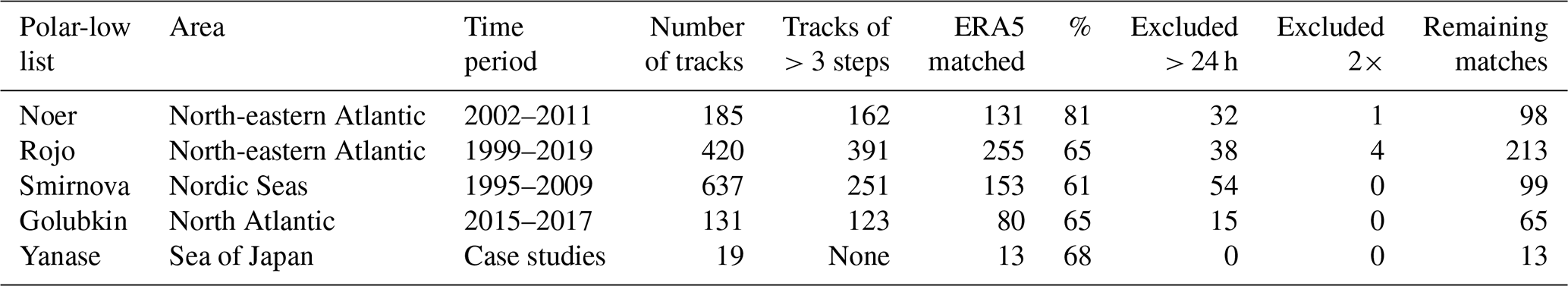
Table 1Match statistics of PLs from the different lists to ERA5 cyclone tracks. The second and third column summarize the area and time period, respectively, covered by the list. Column 4 provides the number of PLs in the lists; column 5 provides the number of PL tracks with more than three time steps, considered necessary for a trustworthy matching. The Yanase list is treated differently, since it provides only one track point per PL. The number and fraction of PLs matched by an ERA5 cyclone track are presented in columns 6 and 7, respectively. A match is obtained if the cyclone track is within a distance of 150 km of the PL for at least half of the track points of the PL. Column 8 displays the amount of matched cases that are excluded, since they start or end more than 24 h earlier or later than the PL from the list. Column 9 shows the number of tracks that are excluded if an ERA5 track matches two PLs from the list. The last column provides the amount of matched PLs included in the parameter derivation.
The Smirnova list provides PLs for the Nordic Seas mainly north of 70∘ N of the years 1995–2009 obtained from a combination of different satellite products (Smirnova et al., 2015). It contains in total 637 PLs, hence more cases per season for a smaller area than the other lists, which indicates the inclusion of weaker systems. Accordingly, only 39 % of the PLs from this list persist for more than three time steps (Table 1), whereas around 90 % of the PLs from the other lists exceed three track points.
The Golubkin list contains 131 PLs of the years 2015–2017 for the whole North Atlantic, including the Labrador Sea, Irminger Sea, and Nordic Seas (Golubkin et al., 2021). It was derived by the inspection of different satellite imagery combined with synoptic-weather charts. The Golubkin, Smirnova, and Rojo lists contain track time steps when the PL was identified on a satellite image, hence at irregular intervals up to 12 h.
The Yanase list is a collection of 19 PLs investigated in the literature in the past 4 decades in the Sea of Japan (Yanase et al., 2016). Different from the other lists, it contains only one time step with a location for each PL such that matching as presented in the next section is challenging. However, this list represents PLs from an ocean basin different than the North Atlantic.
2.3 Track matching
In order to investigate the characteristics of PLs, the ERA5 representations of the PLs from the archives are derived. Only tracks from the PL lists with more than three time steps are considered to ensure a trustworthy track matching. An exception is the Yanase list, since it only provides one time step for each PL.
The following definition for a match is applied: a cyclone matches to a PL if the cyclone track is located within 150 km for at least half of the track points of the PL. This ensures a rather strict spatiotemporal agreement of the tracks but is still flexible for some inaccuracies (i) in the reanalysis to reproduce the PL at the correct location, (ii) in the cyclone tracking algorithm to detect the PL, and (iii) in the location of the PL in the manually derived lists. Different merging distances were tested (Table S1 in the Supplement). A distance of 100 km significantly reduces the detection rate as compared to 150 km distance. A distance of 250 km results in slightly higher detection rates but at a lower quality of the matches.
For all PL lists of the Northern Hemisphere the match rate to ERA5-based cyclone tracks is quite high (Table 1, column 7). More than 80 % of the PLs from the Noer list are matched, as are between 60 % and 70 % for the Rojo, Smirnova, Golubkin, and Yanase lists. The Noer list likely has the highest match rate, since it includes major PL centres that are detected routinely during operational weather prediction, whereas the other lists either include secondary PL centres (e.g. Rojo list) or solely rely on satellite images (e.g. Smirnova list), which both may result in the inclusion of weak systems and problems in the tracking due to large time gaps between images.
The matched tracks to the PL lists are utilized for the derivation of identification criteria for PLs. However, some matched tracks have a considerably longer lifetime than the corresponding track from the PL list (Table 1, column 8). These tracks feature PLs intensifying from a pre-existing circulation anomaly, such as a frontal zone or a renascent of an extra-tropical cyclone. Such transitions are considered part of the life cycle of some PLs and hence are not necessarily false positives. However, systems that are non-PLs for part of their lifetime may distort the derivation of the PL parameters. Therefore, PL-matched cyclone tracks that begin or end 24 h earlier or later, respectively, than the PL from the list are excluded for the parameter derivation. This excludes approximately one-quarter of the matched tracks from the different lists.
A few tracks match two PL tracks, due to multiple PLs with several centres in close vicinity. In such cases, only one matched track is kept, which excludes a few tracks (Table 1, column 9). Manual inspection of the remaining matched PL tracks reveals that they are good representations of the PLs from the lists. For simplicity, the matched PL tracks are in the following only referred to as PLs or PL tracks.
2.4 Parameter derivation
Parameters in the vicinity of the cyclone and PL tracks are investigated. Most parameters are computed as the local mean within 250 km to the centre. To save disc space, the parameters are derived from ERA5 horizontal fields at a 0.5∘ × 0.5∘ grid spacing. The reduced grid spacing was found to produce similar results for the computation of the local averages. Differently, the near-surface wind speed, U10 m, which is computed as the local maxima within 250 km to the cyclone centre, is derived from ERA5 fields at a 0.25∘ × 0.25∘ grid spacing to prevent smoothing of the local wind maxima.
The tropopause is defined by the most common choice as the lowest atmospheric level where 2 PVU (1 PVU = 10−6 K m2 kg−1 s−1; potential vorticity unit) is reached (Kunz et al., 2011). The maximum tropopause wind speed poleward of the system is derived as the maximum value within a band ±0.5∘ longitude and at a latitude with at least the same magnitude as the location of the track.
The parameters are computed for each time step of the track. For the comparison of PL-matched tracks and all cyclone tracks, the lifetime mean, maximum, and minimum are compared, and the most successful is chosen.
The vertical wind shear is derived as in Stoll et al. (2021) based on the differential wind vector, the difference of mean wind vectors at 500 and 925 hPa,
with u and v being the zonal and meridional component of the wind and the overbar denoting a mean computed within a radius of 250 km around the PL centre.3 The vertical-wind-shear strength is then defined by
with z being the geopotential height. The vertical-wind-shear angle is defined as the angle between the differential wind vector, , and the tropospheric mean wind vector, 4,
Different to Stoll et al. (2021), the upper threshold for the weak-shear category is set to 1.0 × 10⁻³ instead of 1.5 × 10⁻³ s−1, since the purposes are different. Stoll et al. (2021) demonstrated differences among the strong shear categories, whereas this study aims to identify the locations in which the shear types occur. However, the results of both studies are robust for the other threshold.
The vortex diameter is estimated by computing the diameter of a circle with the same area as the vortex area, which is the area surrounding the vorticity maxima with ξsmth,850 hPa exceeding 10 × 10−5 s−1 as described in Watanabe et al. (2016) but with a threshold of 12 × 10−5 s−1 in accordance with Stoll et al. (2021). It should be noted that the vortex diameter depends to some degree on the threshold and the smoothness of the vorticity field.
For the comparison in Sect. 3, the parameters for cyclone tracks are derived for only 1 year for each hemisphere to save computational resources. Tests show that the cyclone statistics are robust between years; hence this does not influence the results. For the Northern Hemisphere, 2009 is randomly chosen, and for the Southern Hemisphere, 2004 is taken, since it is the same year as the mesocyclone list of Verezemskaya presented in the Supplement, allowing for the double usage of reanalysis data required for the parameter computation. The parameters utilized for the derivation of the PL climatology (Sect. 4) and for the comparison among PLs (Sect. 5) are derived for the whole time period of ERA5.
Different parameters are compared for their ability to separate between PLs and other cyclones (Table 2 and Figs. 1 and 2). Included are parameters that were found to be successful by Stoll et al. (2018) and new parameters that are expected to capture the characteristics of PLs or their environments. The following consideration is used for the derivation of the PL criteria from the compared parameters: only a small fraction of all cyclone tracks are PLs; hence, a criterion is successful if it holds for most PLs but only for a few cyclones.
Table 2Statistics for the derivation of the polar-low criteria. The type expresses whether the parameter is computed as a lifetime mean, maximum, or minimum of a track. The threshold is chosen such that it is satisfied by 90 % of the polar lows of all five lists. For θ500 hPa−θSST a second threshold satisfying all polar-low lists beside the one from Smirnova is presented. The thresholds noted with an asterisk mark the polar-low criteria. Column 4 expresses the fraction of polar lows from the five lists excluded by the threshold. Column 5 provides the fraction of cyclones excluded by the threshold. The last column displays the additionally excluded cyclones by the threshold after the application of the polar-low criteria of different types. The different types of criteria are separated by vertical lines and labelled with headlines. Utilized abbreviations are the following. N: Noer, R: Rojo, S: Smirnova, Y: Yanase, G: Golubkin, NH: Northern Hemisphere, SH: Southern Hemisphere.
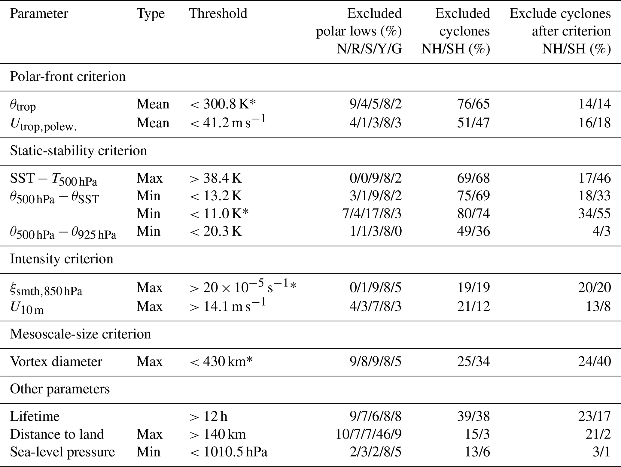
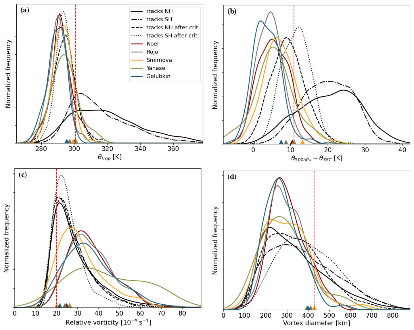
Figure 1Parameter distributions for polar lows from the different lists (colours) and cyclone tracks of both hemispheres (black). These parameters are successful in distinguishing between polar lows and cyclone tracks, hence becoming the polar-low criteria. The tracks that remain after the application of the other three polar-low criteria are presented (black dashed-dotted and dotted) to express the additional value of the parameter to the other three criteria. (a) The potential temperature at the tropopause, θtrop, is computed as the lifetime mean of the track, and (b) the potential static stability, θ500 hPa−θSST, is calculated as the lifetime minimum. (c) The relative vorticity and (d) the vortex diameter express the lifetime maximum. The coloured triangle along the x axis denotes the threshold satisfied by 90 % of the polar lows of each list. The vertical red dashed lines denote the thresholds of the polar-low criteria. NH: Northern Hemisphere, SH: Southern Hemisphere, crit: criteria.

Figure 2As Fig. 1. Parameter distributions for polar lows from the lists (colours) and cyclone tracks of the Northern Hemisphere and Southern Hemisphere (black). Cyclone tracks that remain after the application of the four polar-low criteria for the two hemispheres (black dotted and dashed) are displayed to demonstrate the quality of the polar-low criteria. (a) The maximum wind speed at the tropopause poleward of the system, , is computed as the lifetime mean of the track. (b) The temperature difference between the 500 hPa level and the sea surface, SST−T500 hPa, and (d) the maximum near-surface wind speed, U10 m, as the lifetime maximum. (c) The potential temperature difference between 500 and 925 hPa, θ500 hPa−θ925 hPa, and (f) the sea-level pressure, as the lifetime minimum. (e) The lifetime is the duration of the track.
The threshold for a criterion (Table 2, column 3) is defined such that it excludes less than 10 % of the PLs of all lists (column 4), with an exception for the static-stability criterion explained in Sect. 3.1.2. The skill of a criterion is measured by the fraction of all cyclones it excludes (column 5). The additional value of a criterion is examined by the excluded fraction of cyclones remaining after the application of the other polar-low criteria (column 6).
Further, it is ensured that the criteria consider all the characteristics assigned to PLs by the scientific community, which are intense, mesoscale, and development in marine polar air masses. Another aim is that the PL criteria are successful in all regions and universally applicable to atmospheric models of various resolutions.
The following set of criteria is found to be successful to detect PLs and is in the following called the PL criteria:
-
polar-front criterion of θtrop<300.8 K
-
potential static-stability criterion of K
-
intensity criterion of s−1
-
mesoscale-size criterion of vortex diameter <430 km.
A track that satisfies criterion 1 in the mean of the lifetime, criterion 2 as the minimum, and criteria 3 and 4 as the maximum is defined as a PL track. As noted earlier, PLs sometimes transition from or towards other types of cyclones; hence they are not necessarily PLs for their entire lifetime. Therefore, PL time steps are introduced as the parts of the PL track that satisfy all four criteria simultaneously; 51 % of the time steps from the PL tracks in the Northern Hemisphere and 37 % in the Southern Hemisphere are PL time steps. Most PL tracks satisfy all criteria simultaneously for parts of their lifetime.
The distributions in the parameters utilized for the PL criteria (Fig. 1) are quite similar for the five PL lists from the Northern Hemisphere, expressing that the criteria are independent of the region and the producer of the list. Also, the mesocyclone list of Verezemskaya from the Southern Ocean presented in the Supplement qualitatively agrees with the PL lists, pointing towards general applicability of the PL criteria in both hemispheres. Furthermore, the distributions of the PLs and cyclones are distinct from each other, demonstrating that the parameters are successful for separation.
The derived set of criteria retains most PLs from the five lists (68 %–89 %), whereas only a small fraction of cyclones remains, being 6.7 % for the Northern Hemisphere and 3.6 % for the Southern Hemisphere (Table 3); hence the criteria are quite successful following the consideration at the beginning of this section. These tracks that satisfy the PL criteria form the PL climatology presented in Sect. 4. However, first the individual PL criteria are discussed.
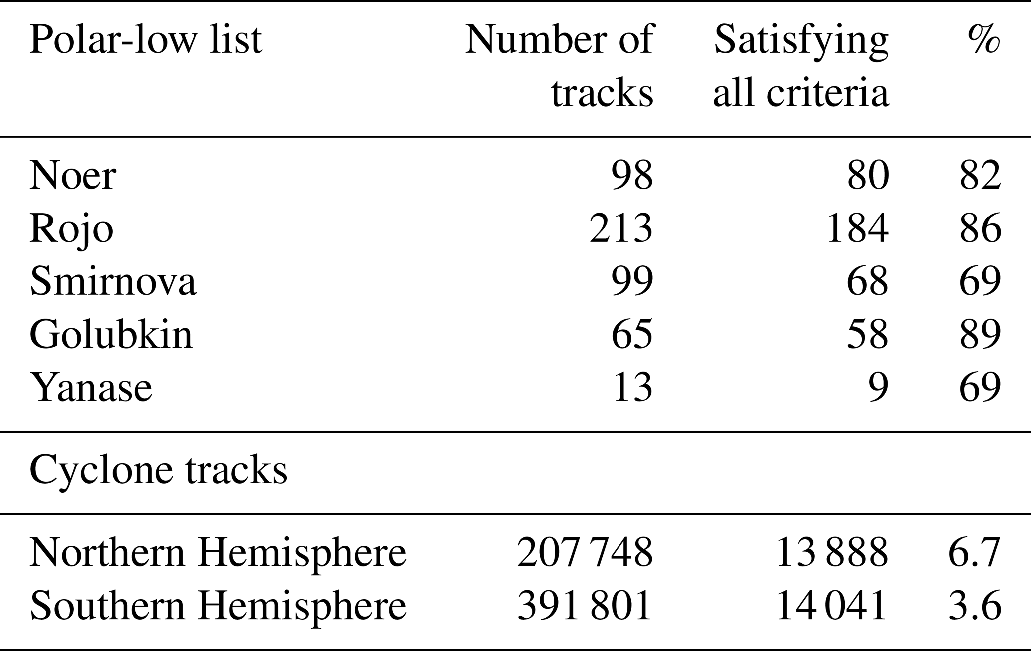
Table 3Statistics for the satisfaction of the polar-low criteria from the polar-low lists and all cyclone tracks of the two hemispheres for the years 1979–2020.
3.1 Marine polar air masses
A guideline for the identification of the marine polar air masses poleward of the main baroclinic zone is not provided by any PL definition. This study exploits two characteristics of the marine polar air masses for its identification: (i) the location poleward of the polar front, leading to criterion 1, and (ii) a low potential dry-static stability, resulting in criterion 2. The two criteria favour each other, which is expressed by a correlation in the parameters for the cyclone tracks in the Northern Hemisphere of 0.73. However, Stoll et al. (2018) demonstrate that approximately one-third of the cyclones with low static stability still feature a considerable jet on the poleward side, therefore utilizing two criteria for the detection of the marine polar air masses. Also, this study finds that two criteria in collaboration are more successful in discriminating between PLs and other cyclones than is a single criterion (see Fig. S1). Further, criteria 1 and 2 are different. Criterion 1 is computed as the lifetime mean; hence it ensures that the PL is in the polar air mass for most of its lifetime. In contrast, criterion 2 is derived as the lifetime minimum and ensures low static stability at least once during the PL development, likely in the intensification phase.
3.1.1 Polar-front criterion
PLs are defined to develop poleward of the polar front (Rasmussen and Turner, 2003). The potential temperature at the tropopause, θtrop, can be used for separation between polar and more temperate air masses. A low potential temperature at the tropopause is reached by a combination of a low temperature at the tropopause and a low altitude of the tropopause, both favoured in polar air masses.
All PL lists agree that the lifetime mean in θtrop is considerably lower for PLs than for most cyclones (Fig. 1a). A threshold that excludes less than 10 % of PLs for all lists is found at 300.8 K (Table 2). The polar-front criterion, θtrop<300.8 K, individually excludes 76 % and 65 % of the Northern Hemisphere and Southern Hemisphere cyclone tracks, respectively, expressing its high value. As mentioned before, this criterion is dependent on the static-stability criterion, but the polar-front criterion excludes an additional 14 % of tracks for both hemispheres (Table 2 and Fig. 1a, dashed and dotted).
Stoll et al. (2018) use the maximum tropopause wind speed poleward of the system, , to identify systems poleward of the polar front. The lifetime mean in is considerably lower for PLs, mainly below 40 m s−1, than for cyclone tracks, where it ranges from 20 to 80 m s−1 (Fig. 2a). Hence, has the potential to separate between PLs and other cyclones but is less successful as an individual criterion than θtrop (Table 2, column 5). Further, distributions in are considerably different across PL lists (Fig. 2a), indicating a local dependence of this criterion, which is less the case for θtrop. For the PLs from the Sea of Japan (Yanase list), the threshold is at 41 m s−1, whereas for lists of PLs in the Nordic Seas (Rojo and Smirnova) the threshold is at 29 m s−1, close to the one used in Stoll et al. (2018). The higher threshold in for the Sea of Japan is likely due to some PLs at the lower latitude of the Sea of Japan occurring in polar air masses characterized with a meandering jet stream such that the jet is located poleward of the system when measured along the same longitude as done for the computation of .
Hence, θtrop is chosen as criterion, since it is shows smaller regional dependency than . The distributions in for the remaining cyclone tracks after the application of the four PL criteria are in good agreement with the distributions of the PLs (Fig. 2a). This expresses that the polar-front characteristics are captured by the PL criteria.
3.1.2 Potential static-stability criterion
Multiple studies have found that PLs form in environments of low dry-static stability through a considerable depth of the troposphere (Forbes and Lottes, 1985; Noer et al., 2011; Stoll et al., 2018; Terpstra et al., 2021). This is applied for the detection of PLs in several studies as a large vertical temperature contrast in the PL environment between the sea surface and the 500 hPa level (SST−T500 hPa; Zahn and von Storch, 2008a; Chen et al., 2014; Zappa et al., 2014; Yanase et al., 2016). Stoll et al. (2018) found that the dry-static stability is superior to the moist-static stability in distinguishing between PLs and other cyclones and that it is more successful when measured between the sea level and the 500 hPa level than when 700 or 850 hPa are used as the upper level. Low dry-static stability is characteristic for the marine polar air masses, since air masses warmed from the sea feature moist-adiabatic lapse rates, which converge towards the dry adiabats at low temperatures typical of the wintertime polar regions (Stoll et al., 2021).
The investigated parameters measuring the static stability, θ500 hPa−θSST, SST−T500 hPa, and θ500 hPa−θ925 hPa, are all found to be successful in distinguishing between PLs and cyclones (Figs. 1b and 2b and c). This confirms that PLs develop in environments of low dry-static stability of considerable depth.
θ500 hPa−θSST and SST−T500 hPa are superior to θ500 hPa−θ925 hPa in excluding cyclone tracks (Table 2). θ500 hPa−θ925 hPa provides a direct measure of the static stability. In contrast, θ500 hPa−θSST and SST−T500 hPa measure the potential static stability of the troposphere. This is “potential” because the sea-surface temperature is considerably warmer than the low-level atmosphere by sometimes 10 K in strong marine cold-air outbreaks (e.g. Papritz et al., 2015). Hence, the two parameters utilizing the SST do not measure the actual static stability of the troposphere but rather the static stability if the lower troposphere would be heated to the temperature of the sea surface. This emphasizes that heating of the lower atmosphere from the sea is characteristic for PL environments. For the sake of simplicity, potential is sometimes dropped in the following.
The two measures for the potential static stability, θ500 hPa−θSST and SST−T500 hPa, are quite similar in the success of excluding cyclone tracks. However, θ500 hPa−θSST is the more universal parameter, since the environmental sea-level pressure appears to be physically irrelevant for PL development (Sect. 3.4) and θ500 hPa−θSST corrects the static stability for pressure variations at sea level. Differently, SST−T500 hPa is prone to seasonal and regional biases by a varying sea-level pressure, as high values are supported by a high sea-level pressure when the vertical distance between the sea surface and the 500 hPa level is large and the lapse rate contributes to the large temperature contrast. When SST−T500 hPa is used, such biases occur in the Southern Ocean, the area of the lowest sea-level pressure globally. Here, SST−T500 hPa excludes considerably more of the remaining cyclones (Table 2: 46 %) than θ500 hPa−θSST (33 %), since the lower sea-level pressure contributes to lower values in SST−T500 hPa such that the SST−T500 hPa criterion is less frequently satisfied in the Southern Hemisphere than the Northern Hemisphere. Hence, for the Southern Ocean a lower threshold should be applied if SST−T500 hPa is utilized, which can be alleviated by using θ500 hPa−θSST.
All PL lists of the Northern Hemisphere beside the one from Smirnova agree on a stricter threshold of K instead of 13.2 K. Also, most PLs from the Smirnova list satisfy this stricter criterion (83 %); however, the Smirnova list includes some cases with considerably higher static stability, which may be false positives. The stricter threshold in θ500 hPa−θSST is considerably more effective in excluding additional cyclones than the weaker threshold of 13.2 K, and therefore it is chosen here.
The distribution of θ500 hPa−θ925 hPa becomes similar for the cyclone tracks satisfying the PL criteria and the PLs from the lists (Fig. 2c), indicating that the PL criteria capture the static-stability characteristics of PLs in addition to the potential static stability.
The threshold of K is approximately equivalent to K for the Northern Hemisphere, but it is approximately at 38 K for PLs in the Southern Ocean, which often features a low sea-level pressure (Fig. 2b and f). Hence, the criterion on the static stability is lower than the threshold of K utilized by multiple studies (Zahn and von Storch, 2008a; Zappa et al., 2014; Yanase et al., 2016). Terpstra et al. (2016) noted that a high static-stability threshold may bias a PL dataset towards reverse-shear cases, since more forward-shear PLs are excluded. The weaker threshold applied here is less prone to biases in shear situations.
3.2 Intensity criterion
PLs are intense mesoscale cyclones. The definition by Rasmussen and Turner (2003) provides an intensity threshold by the near-surface wind speed, U10 m, exceeding 15 m s−1 in the vicinity of the PL, which is commonly used for the detection of PLs (e.g. Zappa et al., 2014; Yanase et al., 2016; Verezemskaya et al., 2017). However, Noer et al. (2011) note that environmental air masses around PLs are frequently advected at a similar velocity. They instead consider the local wind enhancement to measure the intensity of a PL. Accordingly, Stoll et al. (2018) find that the local cyclone depth and the relative vorticity are superior criteria for the PL detection as compared to that of the near-surface wind speed.
The cyclone tracks and the PLs have similar distributions in the near-surface wind speed (Fig. 2d), indicating that U10 m is poor in distinguishing strong from weak mesoscale cyclones being embedded in a strong background flow.
A more successful parameter to measure the intensity of PLs is the smoothed relative vorticity at 850 hPa, ξsmth,850 hPa, which provides a measure of the local vortex strength independent of the background flow. ξsmth,850 hPa is larger for the PLs from the lists than for cyclone tracks (Fig. 1c). The PL lists agree on a threshold s−1, which excludes 20 % of the cyclones for both hemispheres not excluded by the other PL criteria.
Distributions in U10 m are similar for PLs and the tracks satisfying the PL criteria (Fig. 2d), and the threshold of 15 m s−1 defined by Rasmussen and Turner (2003) is mainly satisfied for the tracks satisfying the polar-low criteria. Hence, a near-surface wind criteria is unnecessary for the detection of PLs when a criteria is applied that ensures a strong mesoscale vortex, such as the here-utilized relative vorticity criterion.
3.3 Mesoscale-size criterion
PLs are characterized by their mesoscale size; however, the transition from mesoscale to synoptic-scale cyclones is seamless. The definition by Rasmussen and Turner (2003) specifies a spatial range between 200 and 1000 km. However, observational PL lists contain few systems with diameters larger than 600 km (Rojo et al., 2015; Blechschmidt, 2008). A general method for measuring the size of cyclones across the mesoscale and synoptic-scale is not established. Observational lists typically derive the size from the PL-associated clouds (Rojo et al., 2015). For automation purposes, this approach is problematic when the cyclone intersects with adjacent clouds, often the case in PL environments. Closed pressure contours may be a reasonable measure for synoptic-scale cyclones (e.g. Simmonds and Keay, 2000); however, the pressure contours of mesoscale systems are often distorted by the environmental flow. To circumvent the influence of a uniform background flow, Watanabe et al. (2016) introduce the vortex area defined by the adjacent region with high relative vorticity.
The vortex diameter is generally below 430 km for the PLs from the different lists, whereas it is considerably larger for some cyclone tracks (Fig. 1d). A vortex diameter below 430 km excludes an additional 24 % and 40 % of the cyclones of the Northern Hemisphere and Southern Hemisphere, respectively. Hence, it is a useful criterion for the identification of PLs.
3.4 Comparison to other parameters
Parameters that do not contribute to the PL criteria are compared among the cyclone tracks and the PLs from the lists (Fig. 2). In general, the distributions in these parameters become quite similar regarding the PLs and the tracks which satisfy the PL criteria, which gives confidence that the criteria are skilful. The first four parameters of Fig. 2 were discussed in the previous sections; the remaining are presented in the following.
Surprisingly, the lifetime of cyclones is shorter than for the PLs from the lists (Fig. 2e), even though PLs are known for their rather short lifetime as compared to extra-tropical cyclones. This pinpoints that the tracking algorithm is successful in targeting mesoscale cyclones of a short lifetime. The lifetime of a track is correlated to the maximum intensity of the track (0.44), a criterion for PL identification. This indicates that the PLs are among the mesoscale cyclones of a longer lifetime.
The tracks satisfying the PL criteria have a slightly shorter lifetime than the PLs from the lists. The small difference may be explained by the fact that PLs from the lists being biased towards longer lifetimes, since PLs with less than three time steps are excluded for assuring a trustworthy track matching.
For the Northern Hemisphere, the sea-level pressure of the cyclone tracks is higher than of the PLs (Fig. 2f). However, PLs from the Yanase list have slightly higher sea-level pressure than the cyclones tracks of the Northern Hemisphere. Hence, the distribution in the sea-level pressure is dependent on the region, as noted in the argumentation for choosing θ500 hPa−θSST instead of SST−T500 hPa.
Tracks satisfying the PL criteria have sea-level pressure distributions similar to the PLs of the same hemisphere. This indicates that the tracks captured by the PL criteria feature characteristics similar to the PLs; however, the sea-level pressure is not of value for the detection of PLs.
3.5 Validation: misses and false positives
Since the scientific community does not agree on criteria for the detection of PLs (Moreno-Ibáñez et al., 2021), the estimation of miss and false-positive rates is subjective. Still, estimates in these rates are important for expressing the quality of the derived PL climatology. To the author's knowledge, it is the first time these rates have been estimated for a PL dataset.
First, the degree of subjectivity is demonstrated by a comparison of the manually derived PL lists5 for times and regions of spatiotemporal overlap. The miss and false-positive rates are estimated by defining “list a” as the ground truth. Then cases from list a missing in “list b” are misses, and cases in list b not in list a are false positives. Setting the Rojo list as the ground truth, the Golubkin and Smirnova lists have miss rates of 26 % and 78 % and false-positive rates of 38 % and 74 %, respectively. This expresses that the Rojo and Golubkin lists agree more on their interpretation of a PL and detection method than the Rojo and Smirnova lists.
For the PL climatology, the misses are estimated by combining the match statistics between the PL lists and ERA5 (Table 1) with the fraction of systems satisfying the PL criteria (Table 3). For the different PL lists, 61 % (Smirnova) to 81 % (Noer) of the PLs were matched with a track in ERA5, with the mean of the list being 68 %. From the matched tracks 68 % (Smirnova) to 89 % (Golubkin) satisfy the derived PL criteria, with a mean of the lists being 79 %. Hence, the derived climatology contains between 42 % (Smirnova) and 66 % (Noer) of the PLs from the lists, with a mean of the lists being 54 %. Hence, the climatology misses around 46 % of the PLs from the PL lists. The miss rate appears rather high, however well within the miss rates when different PL lists are compared to each other, as demonstrated above.
The largest contribution to the miss rate is due to the track matching. On average over the lists, 32 % of the PLs do not have a match in ERA5. Possible reasons are that (i) ERA5 does not simulate the PL at the correct location at a sufficient strength, (ii) the tracking procedure is not capable of reproducing the track of every PL, (iii) there is uncertainty in the track location of the PLs from the lists, and (iv) there is some degree of subjectivity as to whether all systems in the lists are clear-cut PLs. All these reasons appear to contribute, whereas quantification of their relative importance is difficult. The applied method for the track matching is rather strict. If the match distance is relaxed from 150 to 250 km, the average match rate of the lists increases from 68 % to 73 % such that the total miss rate decreases from 46 % to 42 %.
The other contribution to the miss rate is the application of the PL criteria, which as mean of the PL lists excludes 21 % of the PLs. Possible reasons include the following: (i) the criteria are too strict, and (ii) there is some degree of subjectivity as to whether all systems in the lists are clear-cut PLs. The method for the derivation of the PL criteria is a compromise between excluding some matched PLs and excluding as many non-PL cyclone tracks as possible (Table 1); hence weaker criteria come at the expanse of more false positives.
For the evaluation of false positives, 100 of the detected PLs were randomly chosen and investigated whether they are considered PLs. For the years 1980 and 2013, 30 and 20 PLs were analysed for the Northern Hemisphere and Southern Hemisphere, respectively, approximately representing the share of PL time steps from the two hemispheres.
The author considers around 80 % of the investigated cases of both hemispheres as reasonable detections of PLs. Around 10 % appear to be false positives, and another 10 % are borderline cases. The false positives are extra-tropical cyclones, frontal zones, and orographically induced shear zones. The borderline cases consist of systems that satisfy the PL criteria only for a short part of their lifetime and originated from or were propagating towards temperate air masses. Some cases are borderline, since they are intense mesoscale cyclones but close to the main baroclinic zone or to the centre of an extra-tropical cyclone.
Additional criteria were tested in order to exclude false cases, such as systems close to land or the remaining few extra-tropical cyclones. However, due to the large variety of the false positives, additional criteria increase the miss rate, with only limited improvement on the false-positive rate.
An estimated miss rate of 46 % and a false-positive rate of 10 %–20 % indicate that the climatology has rather strict criteria which tend to exclude more correct cases than include wrong ones. When considered in the light of disagreement in manually detected PL lists, these rates express that the derived climatology is reasonable.
The PL climatology, consisting of the cyclone tracks that satisfy the four PL criteria, is investigated in this section.
4.1 Spatial distribution of polar lows
Figure 3 shows the spatial distribution of the annual mean PL activity between 1979 and 2020. The PL activity is measured by the number of PL time steps, those satisfying all four PL criteria simultaneously, within a distance of 200 km, which is approximately the mean radius of PLs (Blechschmidt, 2008; Rojo et al., 2015). Hence, this measure of the PL activity estimates the time a location is affected by a PL.
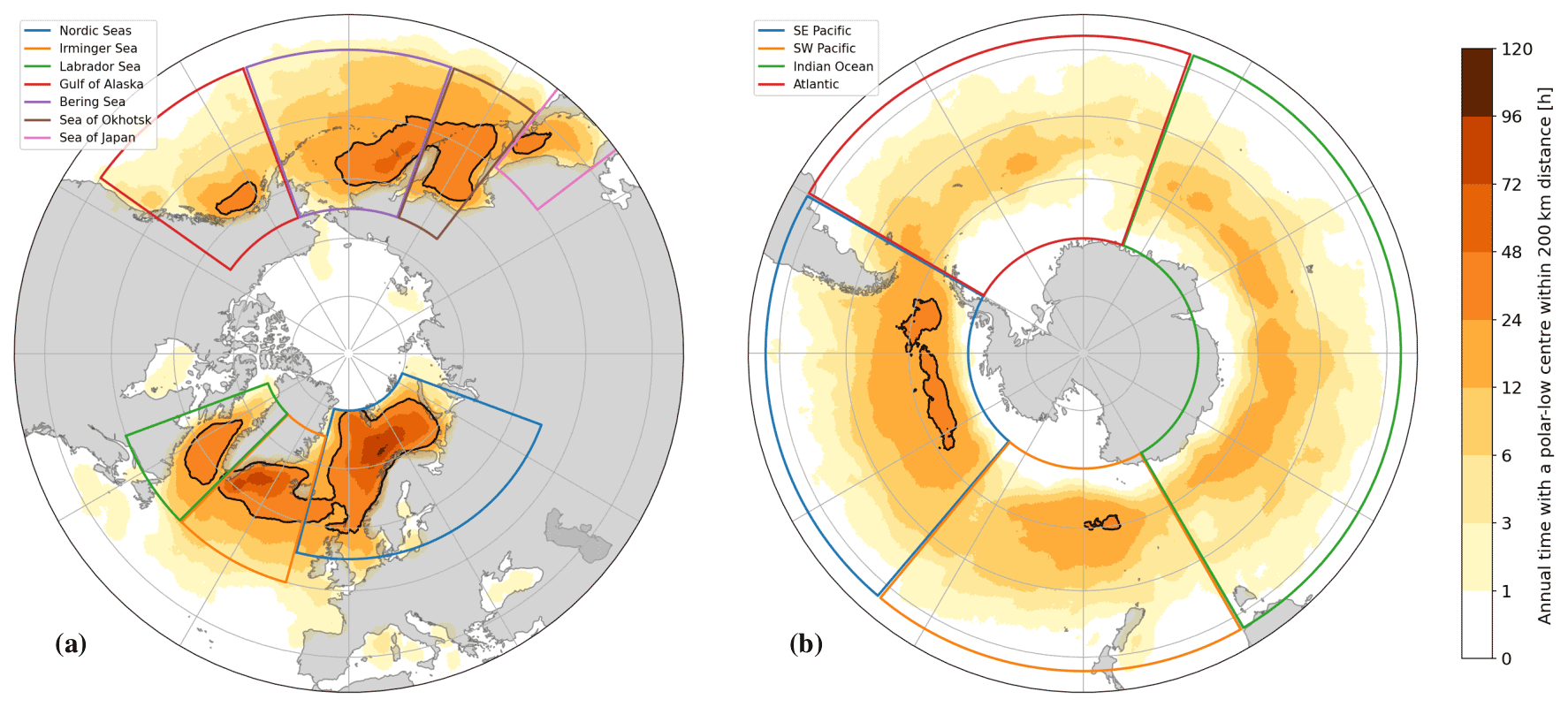
Figure 3Annual mean density of polar-low activity, measured by the amount of polar-low time steps within a 200 km distance, which is a typical radius of a polar low, for (a) the Northern Hemisphere and (b) the Southern Hemisphere. Note the logarithmic colour scale towards low densities. A black contour encircles regions with activity of more than 24 h yr−1, which means that a given location is affected by a polar low with a typical duration of 1 d approximately once per year.
The spatial distribution of the PL activity agrees in many aspects with the climatologies derived from ERA-Interim and the Arctic System Reanalysis (ASR) by Stoll et al. (2018) and with climatologies derived from dynamical downscaling of the National Centers for Environmental Prediction (NCEP) reanalysis for the North Atlantic (Zahn and von Storch, 2008a) and the North Pacific (Chen and von Storch, 2013). This demonstrates the robustness of PL climatologies derived from reanalysis datasets independent of the specific dataset, tracking algorithm, or PL criteria. However, also some improvements are recognized in this climatology.
PLs are observed in all ocean basins at high latitudes. In general, the highest PL activity is found at some 100 km distance from land masses or the sea-ice edge and decays towards the open sea. In the North Atlantic, most PLs appear north of 50∘ N. In the north-western Pacific, considerable PL activity is recognized until 40∘ N. More PLs develop in the western than the eastern Pacific. The most equatorward PLs are found in the Sea of Japan at around 35∘ N. In the Southern Hemisphere, most PLs develop in the latitude band between 50 and 65∘ S.
Increased PL activity occurs in ocean basins semi-enclosed by land or sea ice. Accordingly, the highest density of PLs is in the Nordic Seas, especially between Norway and the Svalbard archipelago, with an average PL activity of 4 d yr−1. This part of the Nordic Seas is known for vigorous PL activity by operational meteorologists (Noer et al., 2011). The second-highest density of PLs is found in the Irminger Sea between Greenland and Iceland up to 3 d yr−1. The Iceland Sea, to the north of Iceland, in between the two most active PL regions, features rather little PL activity of less than 1 d yr−1. In the Pacific, the western Bering Sea is the region of the highest PL activity with 2 d yr−1. Also, a high density of PLs is found in the Sea of Okhotsk, the Labrador Sea, the Gulf of Alaska, and the Sea of Japan with 1–2 d yr−1. All these basins are known for regular PL activity (Yarnal and Henderson, 1989; Golubkin et al., 2021; Yanase et al., 2016).
The climatology includes some PLs in the Hudson Bay; in marginal basins of the Arctic Ocean, being the Kara, Laptev, and Chukchi seas; and in the Mediterranean and the Black Sea. The PL density in these basins is a few hours per year, which means that PLs influence a given location approximately once per decade. These basins are known for their occasional appearance of PLs or related cyclones. In the Hudson Bay, a PL was observed in 1988 (Gachon et al., 2003). In the Chukchi Sea, polar mesoscale cyclones were observed in the open waters of the freezing season (Pichugin et al., 2019). The included PLs in the Mediterranean and the Black Sea are likely medicanes, the Mediterranean sibling of PLs (Businger and Reed, 1989; Romero and Emanuel, 2017). However, the tracking and detection algorithm of this study are not tuned for detecting medicanes and may not capture all of them.
In the Southern Hemisphere, the PL activity is mainly within a latitude band of 65–50∘ S in the vicinity of the sea-ice edge of Antarctica and decays towards more temperate latitudes. The Amundsen Sea in the south-eastern Pacific and a region south of New Zealand in the south-western Pacific feature the highest PL density with more than 1 d yr−1. Generally, the density is considerably lower in the Southern Hemisphere than in its northern counterpart. However, due to a larger ocean area, the total activity is only one-third (37 %) lower. The regions with increased PL activity of the Southern Hemisphere are similar to the areas found by Stoll et al. (2018).
4.1.1 Area of the highest polar-low density
In previous PL climatologies based on reanalysis datasets, the Irminger Sea features the highest density (Zahn et al., 2008; Stoll et al., 2018). However, Golubkin et al. (2021) doubted that the Irminger Sea has a larger PL density than the Nordic Seas by investigation of their manually derived PL list. Accordingly, this climatology has a higher density of PLs in the Nordic Seas than the Irminger Sea, with the latter being the area of the second-highest density globally.
Climatologies of Zahn et al. (2008) and Stoll et al. (2018) likely include a considerable amount of orographically induced shear zones close to the coast of Greenland. Inspection of cases reveals that the here-presented climatology includes only a few shear zones in the Irminger Sea. This observation is supported by a sensitivity study, with the additional exclusion of PL time steps close to land (<200 km), which excludes systems mainly induced by orography. In this sensitivity study, the PL density is reduced not only in the Irminger Sea but also for the other ocean basins such that the Irminger Sea remains the area of the second-highest PL density (Fig. S2). Investigation of the additionally excluded cases reveals that a considerable amount of reasonable PLs are omitted, and hence a criterion using the distance to land is not used for the PL climatology.
4.1.2 Sensitivity climatologies
Sensitivity climatologies are computed in order to test the dependence of the climatology with regard to the threshold in the PL criteria. Four climatologies are derived by making one of the PL criteria stricter but not altering the other three criteria. The strict criterion is determined such that it is satisfied by 70 %–80 % of the PLs from the lists by Noer, Rojo, Yanase, and Golubkin, instead of 90 % of all lists (see Table S2).
For all of the stricter criteria, the fraction of additionally excluded cyclone tracks is higher than that of additional PLs excluded from the lists. Hence, the stricter criteria appear to be successful in the exclusion of borderline cases. Especially increasing the static-stability and the intensity thresholds leads to a large exclusion of additional cyclones.
Generally, the sensitivity climatologies (Fig. S3 and S4) reveal spatial distributions similar to the PL climatology (Fig. 3) with the same areas featuring high activity. This demonstrates that the PL climatology is only a little dependent on the exact threshold in one of the criteria. However, also some differences in the spatial distributions appear and are shortly discussed in the Supplement. This points toward some local differences in the PLs, which is further investigated in Sect. 5.
4.2 Seasonal distribution
The PL climatology, derived based on all months of the year, is able to capture the seasonal distribution (Fig. 4) known from observational studies (e.g. Noer et al., 2011). The reproduction of the seasonality is a good test for the quality of a PL climatology.
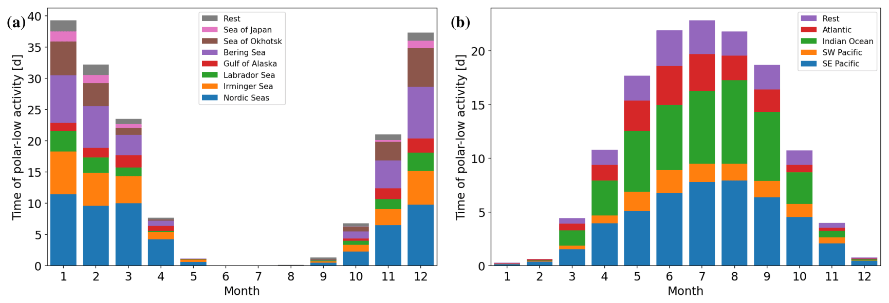
Figure 4The average monthly time of polar-low activity normalized to months with a duration of 30 d for (a) the Northern Hemisphere and (b) the Southern Hemisphere. Given the typical polar-low lifetime of around 24 h, 1 d of activity represents approximately one polar low. Colours denote the contribution of specific regions marked by boxes in Fig. 3.
The displayed seasonal distribution has a large similarity with the one from Stoll et al. (2018) and Chen and von Storch (2013). Generally, PLs develop in the extended winter season of each hemisphere. In the Northern Hemisphere, the main PL season is between November and March with a maximum PL activity in December and January of 37 and 39 d, respectively, hence approximately 40 PLs per month, since PLs have a typical lifetime around 1 d (Fig. 2c and Sect. 5.1). February has a slightly lower activity of 32 d; November and March have activity of approximately 21 and 23 d, respectively. Few PLs develop in October and April with around 7 d of activity per month. In May and September PL development is seldom (1 d per month). In the summer months (June–August) PLs do not develop.
In the Southern Hemisphere, the main PL season is from April to October with a maximum in winter (June–August; up to 23 d), slightly less activity in September (19 d) and May (18 d), and still considerable activity in October and April (11 d). Hence, the main PL season in the Southern Hemisphere is considerably weaker in the peak activity but is 2 months longer than in the Northern Hemisphere. The Southern Ocean features a few PLs in March and November (4 d), considerably more than for the corresponding Northern Hemisphere months of May and September. For the summer months, the PL activity is low in the Southern Hemisphere with less than 1 d per month. In conclusion, the PL activity is weaker in the Southern Hemisphere, less constrained to the winter, and more spread throughout the year.
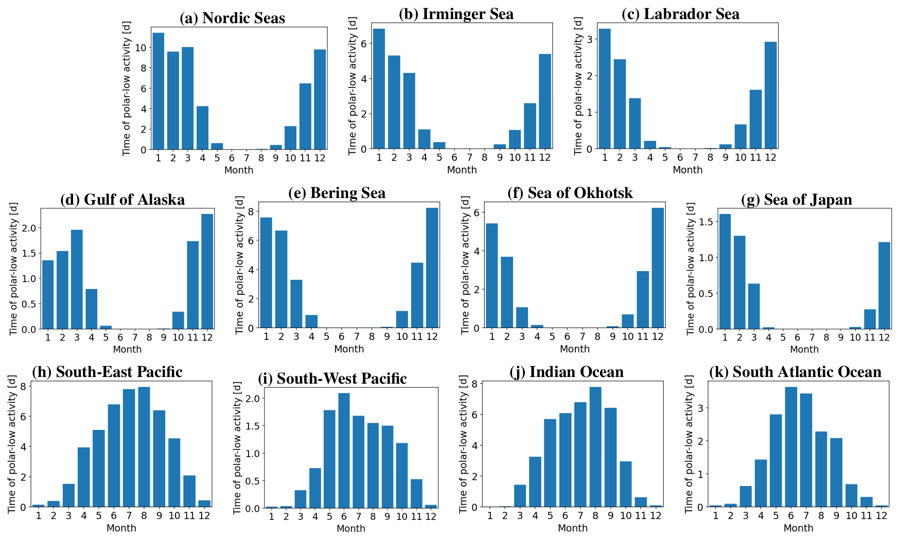
Figure 5The average monthly time of polar-low activity normalized to months with a duration of 30 d for the specific regions marked by boxes in Fig. 3.
The seasonal distribution varies across the ocean sub-basins (Fig. 5). The Nordic Seas have the longest PL season with a plateau of high activity from December to March and considerable activity in November and April. The seasonal distribution is in good agreement with the manually derived PL lists of Noer and Rojo. The season of PL activity is slightly shorter in the Gulf of Alaska and Irminger Sea, with a later start in the former and an earlier end in the latter. In the Labrador Sea and the Bering Sea, most PLs occur in winter from December to February, with some being in November and March. In the Sea of Okhotsk and the Sea of Japan, the PL season is the shortest and mainly constrained to the 3 winter months.
The maximum PL activity is in January for the sub-basins of the North Atlantic as well as for the Sea of Japan. For the other sub-basins of the North Pacific, PL activity peaks in December. The Nordic Seas and the Gulf of Alaska feature a secondary maximum of activity in March, which is weak for the former but significant for the latter.
In the Southern Ocean, the peak in PL activity is different for the ocean basins. In the south-eastern Pacific and the Indian Ocean, most activity occurs in August, and the season is slightly shifted towards the later winter, whereas the south-western Pacific and Atlantic feature the highest activity in June and an earlier season.
The duration and maximum of the local PL seasons are likely influenced by multiple factors, including (i) the availability of ambient cold air masses upstream of the basin; (ii) the occurrence of synoptic-weather patterns advecting the cold air masses over the basin; (iii) the extent of sea ice; and (iv) the sea-surface temperature, which is influenced by ocean currents and the annual cycle.
4.3 Time series, trend, and inter-annual variability
The average annual time of PL activity is 172 d for the Northern Hemisphere and 137 d for the Southern Hemisphere, with an inter-annual variability of 22 and 15 d, respectively (Fig. 6). Note that it is common for multiple PLs to occur simultaneously, where each centre counts to the PL activity.
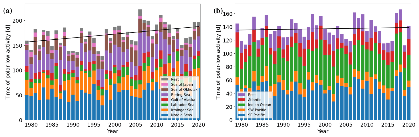
Figure 6The annual time of polar-low activity for (a) the Northern Hemisphere and (b) the Southern Hemisphere. Colours denote the contribution of specific regions marked by boxes in Fig. 3.
In the Southern Hemisphere, the PL activity is rather constant during the investigated period from 1979 to 2020, also for each of the ocean basins. Differently, in the Northern Hemisphere, a significant (p value: 0.006), positive trend in the PL activity of 7.5 d per decade is observed. The largest contribution is from the Nordic Sea and the Labrador Sea, with an increase of 4.1 and 1.9 d per decade, respectively. The positive trend in PL activity is also observed for the sensitivity climatologies, pointing towards the trend being robust for the choice of PL criteria. The trend is significant for the sensitivity climatologies, except for the PLs occurring at low static stability, where the positive trend is weak. This indicates that the choice in the threshold for the static stability may influence observed trends in PL activity.
A comparison with the time series presented in Stoll et al. (2018) reveals that years of high and low PL activity are sometimes in disagreement. Also, the observed trends are different; a decrease in intense PLs as observed by Stoll et al. (2018) is not detected in this climatology. It appears that the observed trends in PL activity should be treated with some caution.
In this section, differences among the PLs from the ocean basins and for the environmental vertical-wind-shear categories are investigated.
5.1 Parameter comparison in the different ocean basins
Generally, PLs from the different ocean sub-basins share many characteristics, expressed by rather similar parameters (Fig. 7), although some differences are apparent. The specific structure and location of an ocean sub-basin can lead to different typical environmental conditions which influence the PL development. Ocean currents likely also influence PL environments in the different ocean basins, but this is not investigated here.
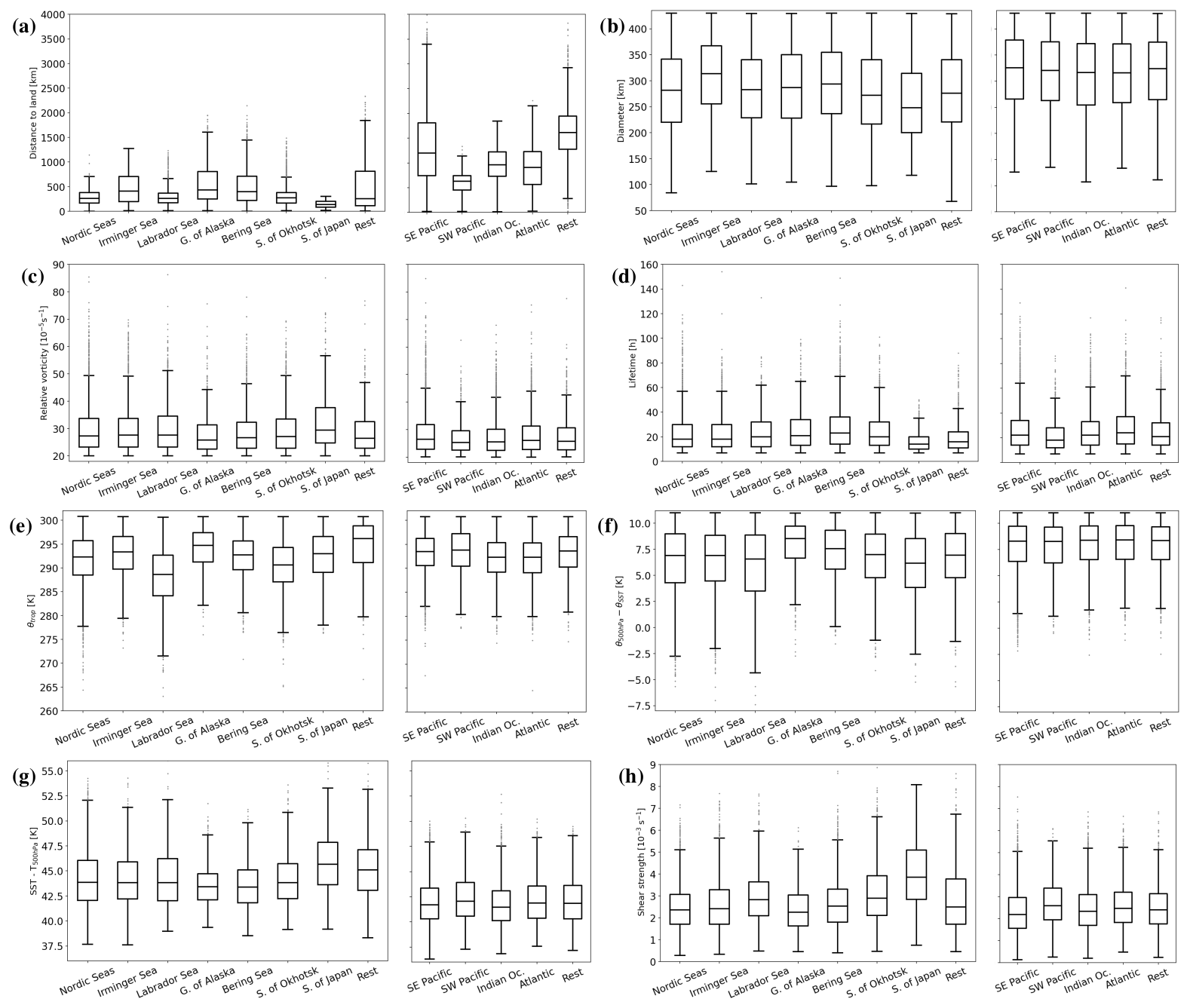
Figure 7Parameter distributions of polar lows for the different regions. The lifetime maximum of the polar-low tracks is used for the computation of (a) the distance to land, (b) the vortex diameter, (c) the relative vorticity, (g) SST−T500 hPa, and (h) the shear strength. For (e) θtrop, the lifetime mean is calculated, and for (f) θ500 hPa−θSST, the lifetime minimum is calculated. (d) The lifetime is the duration of the polar low.
Most PLs occur in close vicinity to land, especially in the Northern Hemisphere (≈500 km; Fig. 7a). This is less the case for the Southern Ocean, since the sea ice around Antarctica creates a buffer between the continent and the open water in which PLs develop. The spatial distribution of PLs for the Southern Hemisphere (Fig. 3b) features the highest density of PLs in the vicinity of the climatological sea ice edge. In the south-western Pacific, the typical distance to land is lower than for the rest of the Southern Ocean, due to the presence of multiple smaller islands. In the Sea of Japan, all PLs occur close to land (<300 km), since it is bounded by continents and islands. Also in the Nordic Seas, the Labrador Sea, and the Sea of Okhotsk, semi-enclosed by continents and islands, the typical distance to land for PLs is around 300 km. The accumulation of PLs in the vicinity of land or sea ice and the fast decay of the PL density at distances larger than 1000 km distance from either of the two (Fig. 3) indicate that for long fetches the marine influence is destroying the polar air masses favourable for PL development.
The typical vortex diameter of PLs is around 300 km (Fig. 7b). PLs in the Southern Hemisphere (median: 320 km) and the Irminger Sea (310 km) are larger, whereas they are smaller in the Sea of Japan (255 km). These size differences are explained by differences in the typical distance to land, which can mask the vortex area of a PL.
The PLs in the climatology have a typical intensity of s−1 (Fig. 7c). They are slightly weaker in the Southern Hemisphere (25 × 10−5 s−1) and stronger in the Sea of Japan (30 × 10−5 s−1). This appears to be an artefact of the vortex area being masked and large vortices tending to have a higher smoothed relative vorticity.
PLs have a typical lifetime of 20 h, ranging between 12 and 32 h (Fig. 7d). PLs often have a longer lifetime in open ocean basins of the Southern Ocean and of the Bering Sea, whereas PLs have a shorter lifetime in the Sea of Japan, surrounded by land. Since PLs are slowly decaying after encountering landfall, the duration is shorter in ocean basins bounded by land.
The typical potential temperature at the tropopause in the PL environments is between 290 and 295 K (Fig. 7e). The median is lower for the Labrador Sea (288 K) and the Sea of Okhotsk (291 K). These ocean basins have continental landmasses to the west and are semi-enclosed by land such that the marine influence is small and that they feature conditions deep in the polar air masses, at low tropopause temperatures.
The potential static stability in PL environments, θ500 hPa−θSST, is typically around 7 K (Fig. 7f). PLs in the Southern Ocean and the Gulf of Alaska feature a slightly higher static stability (8.5 K), and PLs in the Labrador Sea and Sea of Japan have a lower static stability (6 K). When the static stability is measured by SST−T500 hPa, PLs in the Northern Hemisphere feature a typical value of around 44 K, whereas it is lower at 42 K for PLs in the Southern Hemisphere (Fig. 7g). The difference between the hemispheres is larger when using SST−T500 hPa than θ500 hPa−θSST, due to generally lower sea-level pressure in the Southern Ocean at wintertime than anywhere else (Kållberg et al., 2005).
The lifetime maximum in the vertical-wind-shear strength in PL environments is mainly between 2 and 3 × 10⁻³ s−1 (Fig. 7h). The shear is considerably higher for the Sea of Japan, where it has a typical value of 4 × 10⁻³ s−1; slightly higher for the Sea of Okhotsk and the Labrador Sea (3 × 10⁻³ s−1); and lower in the Gulf of Alaska, the south-eastern Pacific, and the Indian Ocean. The next section presents that regions with a higher shear strength feature more forward-shear PLs and that regions with a lower shear strength feature more weak-shear PLs.
5.2 Shear distribution in the different ocean basins
The five different shear categories specified by Stoll et al. (2021) appear in every ocean basin. Note that PLs commonly change their shear category during their development (Stoll et al., 2021); hence the term “forward-shear PLs” captures all polar-low time steps with a forward-shear environment. For both hemispheres, as well as all defined ocean sub-basins, forward-shear PLs are the most common (Figs. 8 and 9), responsible for a third of the time steps (33 % in both hemispheres). Approximately a quarter of the time steps are of weak shear (21 % Northern Hemisphere and 26 % Southern Hemisphere). A slightly lower fraction is of left shear in the Northern Hemisphere (18 %) and right shear in the Southern Hemisphere (25 %), situations where PLs propagate towards warmer environments. Reverse-shear PLs are more common in the Northern Hemisphere (14 %) than in the Southern Hemisphere (7 %). Also, PLs propagating into colder environments are more frequent in the Northern Hemisphere (right shear: 15 %) than in the Southern Hemisphere (left shear: 6 %).
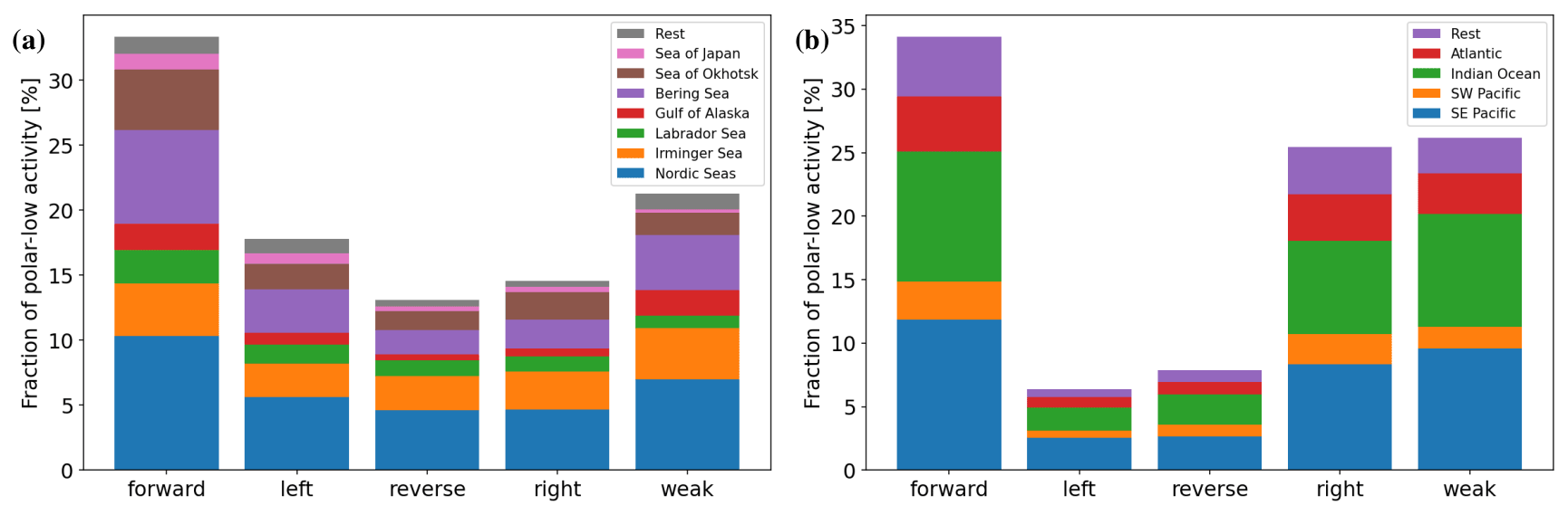
Figure 8Distribution of the different shear categories in the (a) Northern Hemisphere and (b) Southern Hemisphere.
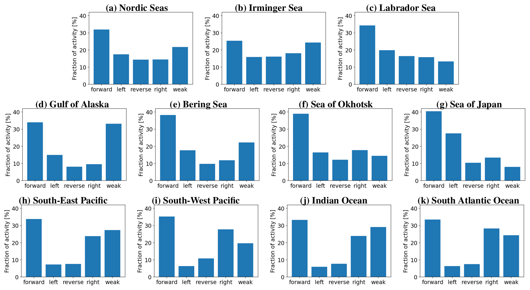
Figure 9Distribution of the different shear categories in the regions marked by boxes in Fig. 3.
Some differences are apparent for the ocean sub-basins. Reverse-shear PLs are more common in the Labrador Sea (16 % of the situations in the basin), Irminger Sea (16 %), and Nordic Seas (14 %) and rather seldom in the Gulf of Alaska (8 %). Forward-shear situations are responsible for a larger fraction in the Sea of Japan (40 %) and the Sea of Okhotsk (39 %) but for a smaller fraction in the Irminger Sea (25 %). Weak shear is more common in the Gulf of Alaska (33 %) and less common in the Sea of Japan (8 %), Labrador Sea (13 %), and Sea of Okhotsk (14 %). The highest fraction of left-shear PLs occurs in the Sea of Japan (27 %) and the Labrador Sea (20 %), likely due to these ocean basins being bounded by land to the west and east which favours northerly, warmward flow.
For the Southern Hemisphere, the most notable difference across the sub-basins is that weak-shear PLs are more common in the south-eastern Pacific (27 %) and the Indian Ocean (29 %) than in the south-western Pacific (20 %) and Atlantic (24 %), while in the latter two regions, right-shear situations are more frequent (28 %) than in the former two (24 %).
The observed increase in PL activity of 7.5 d per decade in the Northern Hemisphere discussed in Sect. 4.3 is mainly due to a significant increase of weak shear (3.2 d per decade), forward-shear (2.8), and reverse-shear PLs (1.0), whereas the number of left and right-shear PLs does not change significantly. In the Southern Hemisphere, the PL activity in all shear classes remains constant.
5.3 Differences in the shear categories
As for PLs in the different ocean sub-basins, PLs associated with the different shear environments share many characteristics (Fig. S5); however, some differences occur (Fig. 10). PLs in forward shear are characterized by considerably stronger shear strength than those in left, right, and reverse shear. Weak-shear systems are by definition of weaker shear strength. The potential static stability, θ500 hPa−θSST, is slightly lower for reverse-shear PLs (median in the Northern Hemisphere: 7.0 K) and PLs propagating towards warmer environments (6.8 K) than for forward shear (7.6 K) and PLs propagating towards colder environments (7.5 K). Hence, there are small differences between the shear categories on how a high baroclinic growth rate is attained.
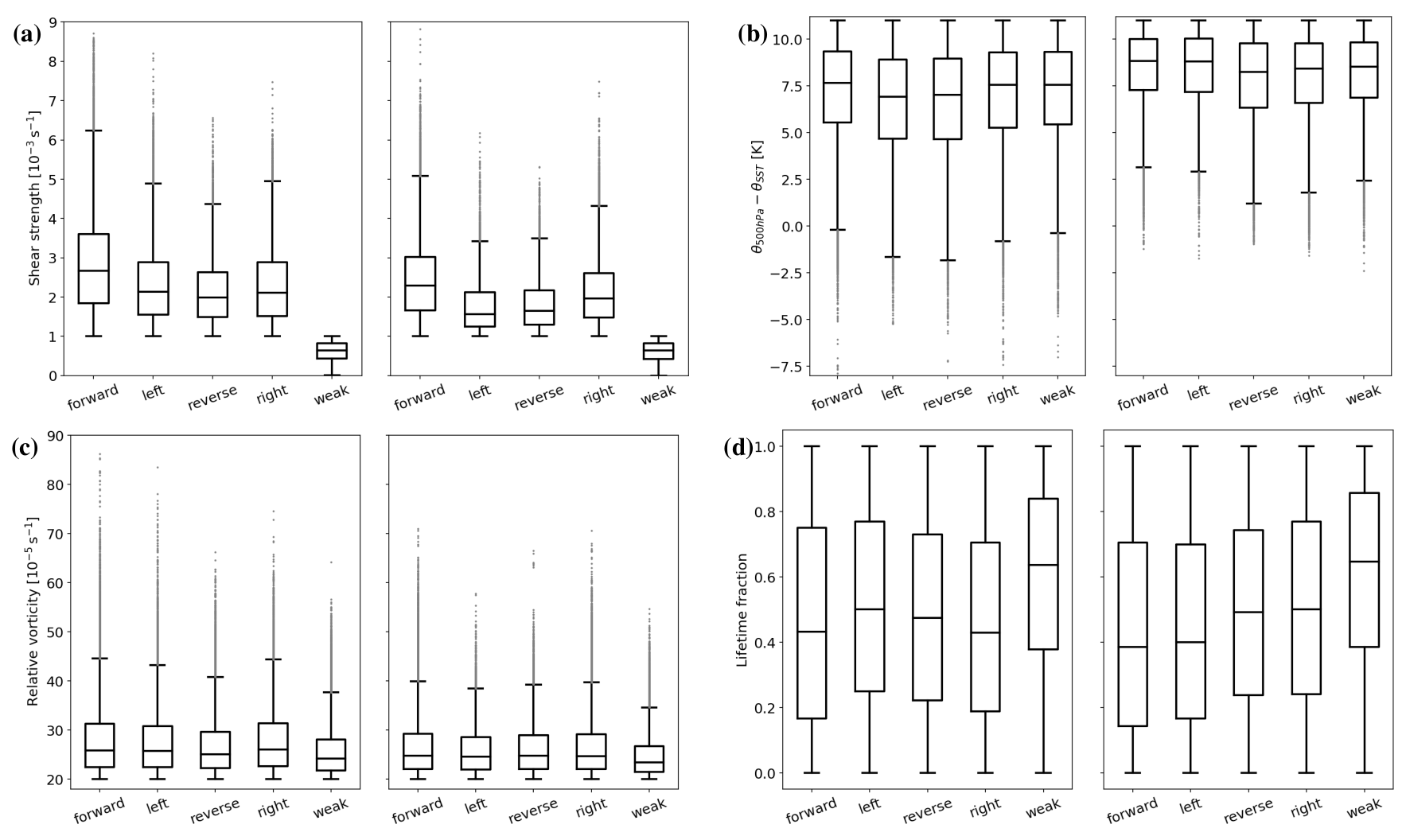
Figure 10Parameter distribution in (a) the vertical-wind-shear strength, (b) the static stability, (c) the relative vorticity, and (d) the lifetime fraction for the different shear categories of (a, c) the Northern Hemisphere and (b, d) the Southern Hemisphere. The parameters are computed for all polar-low time steps within the shear category, since a given polar low often changes shear category during its life. Note that left shear in the Northern Hemisphere and right shear in the Southern Hemisphere are attributed to PLs propagating towards warmer environments.
PLs in environments of weak shear feature static stability similar to the mean of the other strong-shear classes. Hence, convective processes that require a low static stability appear equally important for PLs with a weak shear as for other PLs. The intensity of PLs in a situation of weak shear is slightly lower than of the other shear categories, and weak shear occurs mainly at later stages in the life cycle of PLs. This is all in accordance with Stoll et al. (2021) who hypothesize that weak-shear situations, often associated with spirally formed clouds, are the result of a baroclinic warm-seclusion process.
This study presents a new climatology of PLs based on the ERA5 reanalysis for the years 1979–2020. The criteria for the detection of PLs are derived from a comparison of five PL lists from the literature to mesoscale cyclone tracks derived by a tracking algorithm. The following set of criteria is successful for the identification of PLs: (1) polar-front criterion, θtrop<300.8 K; (2) potential static-stability criterion, K; (3) intensity criterion, s−1; and (4) mesoscale-size criterion, vortex diameter <430 km. These four PL criteria capture the characteristics generally associated with PLs.
The transition between PLs and other types of cyclones is seamless in multiple aspects: the air mass of occurrence, the intensity, and the size. Hence, a specific PL definition is not generally accepted yet (Moreno-Ibáñez et al., 2021), and the classification of a specific phenomenon such as PL can be subjective. However, the meteorological community seems to agree that PLs are extremes within the large variety of cyclones and therefore deserve special attention (Heinemann and Saetra, 2013; Spengler et al., 2017). The lack of a definition complicates the research of PLs. The here-presented PL criteria, derived by comparison of different PL lists by considering the characteristics associated with PLs, provide a specific PL definition. The criteria are generally applicable to gridded datasets and robust towards variations in the thresholds.
The derived PL climatology is trustworthy for multiple reasons. (i) Estimated miss and false-positive rates are reasonable compared to the disagreement of the observational PL list. (ii) Without constraints, the detected PLs satisfy known characteristics, such as a typical lifetime of 15–30 h and near-surface winds stronger than 15 m s−1. (iii) The PL climatology captures known seasonal distributions for individual ocean sub-basins. PLs are winter phenomena, whereas the length of the PL season is considerably different depending on the ocean basin. (iv) For all ocean sub-basins, the PL climatology reproduces spatial distributions in good agreement with observational literature. PLs develop in all ocean basins at high latitude, preferably in close vicinity to land masses or sea ice, in agreement with previous manually and objectively derived PL datasets. Different to previous climatologies based on reanalysis datasets (e.g. Stoll et al., 2018; Zahn and von Storch, 2008a), the Nordic Seas feature the highest density of PLs globally, in agreement with the observational dataset of Golubkin et al. (2021).
For the Northern Hemisphere the climatology captures a significant, positive trend of PL activity, mainly due to an increase in the Nordic Seas and the Labrador Sea. This is different from other climatological studies that observed constant PL activity for the North Atlantic (Stoll et al., 2018; Zahn and von Storch, 2008a) and climate model projections that predict decreasing PL activity for a future warmer climate (Bresson et al., 2022). However, Chen and von Storch (2013) observe a slightly increasing trend of PLs for the North Pacific, using a weaker static-stability criterion. Also, this study uses a rather weak static-stability criterion. The application of a stricter static-stability criterion makes the increase in PL activity become statistically non-significant, pointing towards sensitivity in the PL trend depending on the choice of the static-stability criterion.
This study compares, for the first time, the characteristics of PLs in the different ocean sub-basins. Both the duration of the PL season and the month of maximum activity vary among the sub-basins. However, the PLs share many characteristics across ocean basin, such as the intensity, size, lifetime, and parameters of the environmental air masses. Differences are explained by the specific configurations of the basin. For example, PLs in the Sea of Japan and the Labrador Sea develop more often in environments of lower static stability, whereas PLs in the Southern Ocean and the Gulf of Alaska occur in slightly more stable environments. In the former regions, the upstream air is often influenced by a long fetch over the wintertime cold continent; hence the air mass has time to cool, whereas the latter region is more maritime influenced. Generally, the variability of PLs within each basin is larger than the difference between PLs of the different basins.
This study also globally investigates the fraction of PLs in different vertical-wind-shear environments. The five vertical-wind-shear categories derived by Stoll et al. (2021) occur in all regions of PL activity. Forward-shear PLs are the most common everywhere, responsible for 25 % (Irminger Sea) to 41 % (Sea of Japan) of the PL time steps. PLs in weak-shear environments occur in 22 % and 26 % of the time for the Northern Hemisphere and Southern Hemisphere, respectively. Weak-shear PLs are seldom in the Sea of Japan, the Sea of Okhotsk, and the Labrador Sea (8 %–14 %) but rather frequent in the Gulf of Alaska and the Indian Ocean (29 %–33 %).
PLs propagating towards warmer environments, being of left shear in the Northern Hemisphere (18 %) and right shear in the Southern Hemisphere (25 %), are also quite common. Reverse-shear PLs are rather seldom; however, they are more common in the Northern Hemisphere (14 %) than the Southern Hemisphere (7 %). PLs propagating towards colder environments are of approximately similar occurrence to reverse-shear PLs in both hemispheres. Also for these two shear types, considerable regional differences in the frequency exist. They have the highest shares in the North Atlantic and the Sea of Okhotsk.
Most environmental parameters are quite similar for the shear categories, and differences are in accordance with Stoll et al. (2021). The shear strength is often larger for forward-shear PLs, whereas the static stability is often lower for reverse-shear PLs and the PLs propagating towards warmer environments. Hence, the contributors to a high baroclinic growth rate are slightly different within the strong-shear categories. Weak-shear situations mainly occur in the decaying phase of the PL, indicating that the intensification of PLs requires environmental baroclinicity.
The polar-low climatology and the ERA5 tracks matched to the PL lists are provided at https://doi.org/10.18710/TVZDBF (Stoll, 2022a). They contain the environmental parameters used in this study.
A video supplement is available at https://doi.org/10.5446/56711 (Stoll, 2022b).
The supplement related to this article is available online at: https://doi.org/10.5194/wcd-3-483-2022-supplement.
The contact author has declared that there are no competing interests.
Publisher’s note: Copernicus Publications remains neutral with regard to jurisdictional claims in published maps and institutional affiliations.
Thanks go to ECMWF for providing access to data from the ERA5 reanalysis. The data were processed using the supercomputer FRAM and stored at NIRD, both provided by the Norwegian Research Infrastructure Services (NRIS) Sigma2 AS under the projects NN9348K and NS9063K, respectively. Three anonymous reviewers are also thanked for their constructive comments which considerably improved the paper.
This paper was edited by Helen Dacre and reviewed by three anonymous referees.
Blechschmidt, A.-M.: A 2-year climatology of polar low events over the Nordic Seas from satellite remote sensing, Geophys. Res. Lett., 35, L09815, https://doi.org/10.1029/2008GL033706, 2008. a, b
Bracegirdle, T. J. and Gray, S. L.: An objective climatology of the dynamical forcing of polar lows in the Nordic seas, Int. J. Climatol., 28, 1903–1919, 2008. a, b, c
Bresson, H., Hodges, K. I., Shaffrey, L. C., Zappa, G., and Schiemann, R.: The response of Northern Hemisphere polar lows to climate change in a 25 km high-resolution global climate model, J. Geophys. Res.-Atmos., 127, e2021JD035610, https://doi.org/10.1029/2021JD035610, 2022. a
Bromwich, D. H., Wilson, A. B., Bai, L.-S., Moore, G. W. K., and Bauer, P.: A comparison of the regional Arctic System Reanalysis and the global ERA-Interim Reanalysis for the Arctic, Q. J. Roy. Meteor. Soc., 142, 644–658, 2016. a
Businger, S. and Reed, R. J.: Cyclogenesis in cold air masses, Weather Forecast., 4, 133–156, 1989. a
Chang, C.-C., Wang, Z., Walsh, J., and Stoll, P. J.: Modulation of North Atlantic Polar Low Activity by Sudden Stratospheric Warmings, J. Climate, https://doi.org/10.1175/JCLI-D-21-0905.1, online first, 2022. a
Chen, F. and von Storch, H.: Trends and variability of North Pacific polar lows, Adv. Meteorol., 2013, 170387, https://doi.org/10.1155/2013/170387, 2013. a, b, c, d
Chen, F., von Storch, H., Zeng, L., and Du, Y.: Polar Low genesis over the North Pacific under different global warming scenarios, Clim. Dynam., 43, 3449–3456, 2014. a
Dee, D. P., Uppala, S. M., Simmons, A. J., Berrisford, P., Poli, P., Kobayashi, S., Andrae, U., Balmaseda, M. A., Balsamo, G., Bauer, P., Bechtold, P., Beljaars, A. C. M., van de Berg, L., Bidlot, J., Bormann, N., Delsol, C., Dragani, R., Fuentes, M., Geer, A. J., Haimberger, L., Healy, S. B., Hersbach, H., Hólm, E. V., Isaksen, L., Kållberg, P., Köhler, M., Matricardi, M., McNally, A. P., Monge-Sanz, B. M., Morcrette, J.-J., Park, B.-K., Peubey, C., de Rosnay, P., Tavolato, C., Thépaut, J.-N., and Vitart, F.: The ERA-Interim reanalysis: Configuration and performance of the data assimilation system, Q. J. Roy. Meteor. Soc., 137, 553–597, 2011. a
Duncan, C.: Baroclinic instability in a reversed shear-flow, Meteorol. Mag., 107, 17–23, 1978. a
Forbes, G. S. and Lottes, W. D.: Classification of mesoscale vortices in polar airstreams and the influence of the large-scale environment on their evolutions, Tellus A, 37, 132–155, 1985. a
Gachon, P., Laprise, R., Zwack, P., and Saucier, F. J.: The effects of interactions between surface forcings in the development of a model-simulated polar low in Hudson Bay, Tellus A, 55, 61–87, 2003. a
Golubkin, P., Smirnova, J., and Bobylev, L.: Satellite-Derived Spatio-Temporal Distribution and Parameters of North Atlantic Polar Lows for 2015–2017, Atmosphere, 12, 224, https://doi.org/10.3390/atmos12020224, 2021. a, b, c, d, e, f
Harrold, T. and Browning, K.: The polar low as a baroclinic disturbance, Q. J. Roy. Meteor. Soc., 95, 710–723, 1969. a
Heinemann, G. and Saetra, Ø.: Workshop on polar lows, B. Am. Meteorol. Soc., 94, ES123–ES126, 2013. a
Hersbach, H., Bell, B., Berrisford, P., Hirahara, S., Horányi, A., Muñoz-Sabater, J., Nicolas, J., Peubey, C., Radu, R., Schepers, D., Simmons, A., Soci, C., Abdalla, S., Abellan, X., Balsamo, G., Bechtold, P., Biavati, G., Bidlot, J., Bonavita, M., De Chiara, G., Dahlgren, P., Dee, D., Diamantakis, M., Dragani, R., Flemming, J., Forbes, R., Fuentes, M., Geer, A., Haimberger, L., Healy, S., Hogan, R. J., Hólm, E., Janisková, M., Keeley, S., Laloyaux, P., Lopez, P., Lupu, C., Radnoti, G., de Rosnay, P., Rozum, I., Vamborg, F., Villaume, S., and Thépaut, J.-N.: The ERA5 global reanalysis, Q. J. Roy. Meteor. Soc., 146, 1999–2049, 2020. a, b
Kållberg, P., Berrisford, P., Hoskins, B., Simmons, A., Lamy-thépaut, S., and Hine, R.: ERA-40 atlas, ECMWF, https://sites.ecmwf.int/era/40-atlas/docs/index.html (last access: 31 March 2022), 2005. a
Kunz, A., Konopka, P., Müller, R., and Pan, L.: Dynamical tropopause based on isentropic potential vorticity gradients, J. Geophys. Res.-Atmos., 116, D01110, https://doi.org/10.1029/2010JD014343, 2011. a
Laffineur, T., Claud, C., Chaboureau, J.-P., and Noer, G.: Polar lows over the Nordic Seas: Improved representation in ERA-Interim compared to ERA-40 and the impact on downscaled simulations, Mon. Weather Rev., 142, 2271–2289, 2014. a, b
Michel, C., Terpstra, A., and Spengler, T.: Polar Mesoscale Cyclone Climatology for the Nordic Seas Based on ERA-Interim, J. Climate, 31, 2511–2532, 2018. a, b, c, d, e
Moreno-Ibáñez, M., Laprise, R., and Gachon, P.: Recent advances in polar low research: current knowledge, challenges and future perspectives, Tellus A, 73, 1–31, 2021. a, b, c, d
Noer, G., Saetra, Ø., Lien, T., and Gusdal, Y.: A climatological study of polar lows in the Nordic Seas, Q. J. Roy. Meteor. Soc., 137, 1762–1772, 2011. a, b, c, d, e, f
Orimolade, A., Furevik, B., Noer, G., Gudmestad, O., and Samelson, R.: Waves in polar lows, J. Geophys. Res.-Oceans, 121, 6470–6481, 2016. a
Papritz, L., Pfahl, S., Sodemann, H., and Wernli, H.: A climatology of cold air outbreaks and their impact on air–sea heat fluxes in the high-latitude South Pacific, J. Climate, 28, 342–364, 2015. a
Pichugin, M. K., Gurvich, I. A., and Zabolotskikh, E. V.: Severe Marine Weather Systems During Freeze-Up in the Chukchi Sea: Cold-Air Outbreak and Mesocyclone Case Studies From Satellite Multisensor Measurements and Reanalysis Datasets, IEEE J. Sel. Top. Appl., 12, 3208–3218, 2019. a
Rasmussen, E. A. and Turner, J.: Polar lows: Mesoscale Weather Systems in the Polar Regions, Cambridge University Press, ISBN 978-0521183918, 2003. a, b, c, d, e, f
Renfrew, I.: Synoptic Meteorology, Polar Lows, in: Encyclopedia of Atmospheric Sciences (Second Edition), edited by: North, G. R., Pyle, J., and Zhang, F., Academic Press, Oxford, 379–385, https://doi.org/10.1016/B978-0-12-382225-3.00317-0, 2015. a, b
Rojo, M., Claud, C., Mallet, P.-E., Noer, G., Carleton, A. M., and Vicomte, M.: Polar low tracks over the Nordic Seas: a 14-winter climatic analysis, Tellus A, 67, 24660, https://doi.org/10.3402/tellusa.v67.24660, 2015. a, b, c, d, e
Rojo, M., Claud, C., Noer, G., and Carleton, A. M.: In situ measurements of surface winds, waves, and sea state in polar lows over the North Atlantic, J. Geophys. Res.-Atmos., 124, 700–718, 2019a. a
Rojo, M., Noer, G., and Claud, C.: Polar Low tracks in the Norwegian Sea and the Barents Sea from 1999 until 2019, PANGAEA [data set], https://doi.org/10.1594/PANGAEA.903058, 2019b. a
Romero, R. and Emanuel, K.: Climate Change and Hurricane-Like Extratropical Cyclones: Projections for North Atlantic Polar Lows and Medicanes Based on CMIP5 Models, J. Climate, 30, 279–299, 2017. a
Samuelsen, E. M., Løset, S., and Edvardsen, K.: Marine icing observed on KV Nordkapp during a cold air outbreak with a developing polar low in the Barents sea, Proceedings of the 23rd International Conference on Port and Ocean Engineering under Arctic Conditions, 14–18 June 2015, Trondheim, Norway, https://hdl.handle.net/10037/8583 (last access: 1 April 2022), 2015. a
Simmonds, I. and Keay, K.: Mean Southern Hemisphere extratropical cyclone behavior in the 40-year NCEP–NCAR reanalysis, J. Climate, 13, 873–885, 2000. a
Smirnova, J. E. and Golubkin, P. A.: Comparing polar lows in atmospheric reanalyses: Arctic System Reanalysis versus ERA-Interim, Mon. Weather Rev., 145, 2375–2383, 2017. a, b, c
Smirnova, J. E., Golubkin, P. A., Bobylev, L. P., Zabolotskikh, E. V., and Chapron, B.: Polar low climatology over the Nordic and Barents seas based on satellite passive microwave data, Geophys. Res. Lett., 42, 5603–5609, 2015. a, b
Spengler, T., Claud, C., and Heinemann, G.: Polar Low Workshop Summary, B. Am. Meteorol. Soc., 98, ES139–ES142, 2017. a
Stoll, P. J.: Background Data for: A global climatology of polar lows investigated for local differences and wind-shear environments, DataverseNO, V1 [data set], https://doi.org/10.18710/TVZDBF, 2022a. a
Stoll, P. J.: A global climatology of polar lows investigated for local differences and wind-shear environments, TIB AV-Portal [video], https://doi.org/10.5446/56711, 2022b. a
Stoll, P. J., Graversen, R. G., Noer, G., and Hodges, K.: An objective global climatology of polar lows based on reanalysis data, Q. J. Roy. Meteor. Soc., 144, 2099–2117, 2018. a, b, c, d, e, f, g, h, i, j, k, l, m, n, o, p, q, r, s, t, u, v, w, x, y, z
Stoll, P. J., Spengler, T., Terpstra, A., and Graversen, R. G.: Polar lows – moist-baroclinic cyclones developing in four different vertical wind shear environments, Weather Clim. Dynam., 2, 19–36, https://doi.org/10.5194/wcd-2-19-2021, 2021. a, b, c, d, e, f, g, h, i, j, k, l, m, n, o, p, q, r, s
Terpstra, A. and Watanabe, S.-I.: Polar Lows, in: Climate Science, Oxford Research Encyclopedia, https://doi.org/10.1093/acrefore/9780190228620.013.775, 2020. a, b
Terpstra, A., Michel, C., and Spengler, T.: Forward and reverse shear environments during polar low genesis over the North East Atlantic, Mon. Weather Rev., 144, 1341–1354, 2016. a, b, c, d
Terpstra, A., Renfrew, I. A., and Sergeev, D. E.: Characteristics of Cold-Air Outbreak Events and Associated Polar Mesoscale Cyclogenesis over the North Atlantic Region, J. Climate, 34, 4567–4584, 2021. a
Verezemskaya, P., Tilinina, N., Gulev, S., Renfrew, I. A., and Lazzara, M.: Southern Ocean mesocyclones and polar lows from manually tracked satellite mosaics, Geophys. Res. Lett., 44, 7985–7993, 2017. a, b
Watanabe, S.-I. I., Niino, H., and Yanase, W.: Climatology of polar mesocyclones over the Sea of Japan using a new objective tracking method, Mon. Weather Rev., 144, 2503–2515, 2016. a, b, c, d, e, f
Wilhelmsen, K.: Climatological study of gale-producing polar lows near Norway, Tellus A, 37, 451–459, 1985. a
Yanase, W., Niino, H., Watanabe, S.-I. I., Hodges, K., Zahn, M., Spengler, T., and Gurvich, I. A.: Climatology of polar lows over the Sea of Japan using the JRA-55 reanalysis, J. Climate, 29, 419–437, 2016. a, b, c, d, e, f, g, h
Yarnal, B. and Henderson, K. G.: A climatology of polar low cyclogenetic regions over the North Pacific Ocean, J. Climate, 2, 1476–1491, 1989. a
Zahn, M. and von Storch, H.: A long-term climatology of North Atlantic polar lows, Geophys. Res. Lett., 35, L22702, https://doi.org/10.1029/2008GL035769, 2008a. a, b, c, d, e, f, g
Zahn, M. and von Storch, H.: Tracking polar lows in CLM, Meteorol. Z., 17, 445–453, 2008b. a
Zahn, M., von Storch, H., and Bakan, S.: Climate mode simulation of North Atlantic polar lows in a limited area model, Tellus A, 60, 620–631, 2008. a, b, c
Zappa, G., Shaffrey, L., and Hodges, K.: Can polar lows be objectively identified and tracked in the ECMWF operational analysis and the ERA-Interim reanalysis?, Mon. Weather Rev., 142, 2596–2608, 2014. a, b, c, d, e, f, g
Stoll et al. (2021) merged the closest vorticity maxima within 100 km, but some testing found the applied values to be slightly superior for this study.
The radius of 250 km is different to the radius of 500 km utilized by Stoll et al. (2021). Both radii were compared, and the results are in good agreement, but the smaller radius appears to better represent the local environment.
This definition is in close agreement with Terpstra et al. (2016), who compute the angle between the mean and the thermal wind. It differs from Stoll et al. (2021), who analyse PLs from the perspective of their propagation and therefore utilize the propagation direction of the PL instead of the mean wind. However, Stoll et al. (2021) argue that the mean tropospheric wind provides a good estimate of the propagation direction of PLs, and hence both methods are expected to give similar results. Differences in the propagation direction and the orientation of the mean tropospheric wind vector can occur in situations of slow propagation associated with weak environmental winds.
To be precise, the ERA5 tracks matched to the lists are compared.