the Creative Commons Attribution 4.0 License.
the Creative Commons Attribution 4.0 License.
 | 11 May 2022
Summertime changes in climate extremes over the peripheral Arctic regions after a sudden sea ice retreat
Thierry Fichefet
François Massonnet
David Docquier
Rym Msadek
Svenya Chripko
Christopher Roberts
Sarah Keeley
Retish Senan
The retreat of Arctic sea ice is frequently considered to be a possible driver of changes in climate extremes in the Arctic and possibly down to mid-latitudes. However, it remains unclear how the atmosphere will respond to a near-total retreat of summer Arctic sea ice, a reality that might occur in the foreseeable future. This study explores this question by conducting sensitivity experiments with two global coupled climate models run at two different horizontal resolutions to investigate the change in temperature and precipitation extremes during summer over peripheral Arctic regions following a sudden reduction in summer Arctic sea ice cover. An increase in frequency and persistence of maximum surface air temperature is found in all peripheral Arctic regions during the summer, when sea ice loss occurs. For each 1×10⁶ km2 of Arctic sea ice extent reduction, the absolute frequency of days exceeding the surface air temperature of the climatological 90th percentile increases by ∼ 4 % over the Svalbard area, and the duration of warm spells increases by ∼ 1 d per month over the same region. Furthermore, we find that the 10th percentile of surface daily air temperature increases more than the 90th percentile, leading to a weakened diurnal cycle of surface air temperature. Finally, an increase in extreme precipitation, which is less robust than the increase in extreme temperatures, is found in all regions in summer. These findings suggest that a sudden retreat of summer Arctic sea ice clearly impacts the extremes in maximum surface air temperature and precipitation over the peripheral Arctic regions with the largest influence over inhabited islands such as Svalbard or northern Canada. Nonetheless, even with a large sea ice reduction in regions close to the North Pole, the local precipitation response is relatively small compared to internal climate variability.
- Article
(10661 KB) - Full-text XML
- BibTeX
- EndNote


Arctic sea ice extent has been decreasing since the beginning of satellite observations in 1979. This decrease has occurred in all seasons but is more pronounced in late summer. In particular, September sea ice extent has shrunk by about 50 % since the beginning of the satellite era (Onarheim et al., 2018). The loss of sea ice, which is largely attributed to the accumulation of greenhouse gases in the atmosphere following anthropogenic emissions (Notz and Stroeve, 2016; Screen et al., 2018) but also to internal climate variability (Ding et al., 2017), has been proposed as a key driver of “Arctic amplification” (AA) through changes in albedo (Manabe and Stouffer, 1994; Screen and Simmonds, 2010) and other temperature-related feedbacks (Pithan and Mauritsen, 2014).
To investigate the role of the sea ice retreat on climate, observations are not sufficient (Smith et al., 2019). Indeed, sea ice and atmospheric circulation might be related to each other in the observational record, but this relationship could have occurred by chance. The relationship could also be non-causal, especially if both sea ice and the atmospheric circulation are driven by a common factor (Blackport et al., 2019). To overcome these problems, the use of numerical model experiments, in which a retreat of summer Arctic sea ice can be imposed, is an attractive approach to determining the influence of sea ice anomalies on the climate system. However, even with exactly the same experimental setup, significant differences in the mid-latitude responses are found within the same model, suggesting that internal climate variability to Arctic sea ice loss can play a large role (Peings et al., 2021).
The winter climate response to a summer Arctic sea ice loss and/or AA have garnered a lot of attention (e.g. Francis and Vavrus, 2012; Cohen et al., 2014; Barnes and Screen, 2015; Cohen et al., 2020). So far these responses have mostly been studied for mid-latitude regions (Ogawa et al., 2018). A large uncertainty in the dynamical aspects of the climate response to Arctic sea ice loss in mid-latitudes (Coumou et al., 2018) can also be observed in summer, when the role of the stratosphere is negligible (Kidston et al., 2015). However, the climate response near the regions of Arctic sea ice loss depends primarily on the surface heat flux changes (e.g. Deser et al., 2010) and is therefore less dependent on internal climate variability than at mid-latitudes. Thereby, the ratio of the signal (response of the atmosphere to sea ice loss) to noise (internally generated variability) over the peripheral Arctic regions is larger, and fewer ensemble members are needed to get a significant response compared to mid-latitude regions (Screen et al., 2014). Studies focusing on the summer response of the atmosphere to sea ice reductions and/or AA have been restricted to mid-latitude regions (Horton et al., 2016; Coumou et al., 2018).
In summer, the dynamical and thermodynamical aspects both could tend to lead to more extreme weather events such as hot extremes (Horton et al., 2016). An increase in climate extremes (frequency, intensity or persistence) can have greater impacts on human activities and on the natural environment than an increase in the climatic mean (Kunkel et al., 1999). Over the last decades, extreme heat events have increased in the Arctic regions mainly over the Arctic North America and Greenland (Matthes et al., 2015; Dobricic et al., 2020), and Arctic aridity has decreased (Meredith et al., 2019). These changes are already impacting the Arctic regions, with a change in fish stocks (Hollowed et al., 2013; Haug et al., 2017) and in agriculture (Stevenson et al., 2014), and posing risks to local communities (Ford et al., 2008). Moreover, a “new Arctic” climate could even emerge during this century (Landrum and Holland, 2020). Indeed, a larger decrease in magnitude in cold extremes compared to the increase in warm extremes and an increase in precipitation extremes are expected over high latitudes (Kharin et al., 2013; Sillmann et al., 2013b). The projected Arctic sea ice loss could be responsible for this decrease in temperature variance (Blackport et al., 2021) and in the increase in precipitation extremes, but with a significant difference between regions (Screen et al., 2015).
Even if the rate of summer Arctic sea ice decline is not uniform and might be slowed down for a few years depending on the effect of internal climate variability (Swart et al., 2015), sudden reductions in Arctic sea ice extent are likely to be more frequent in the future, with sea ice retreating 4 times faster than the long-term trend (Holland et al., 2006). Moreover, many state-of-the-art climate models project summer ice-free Arctic conditions before 2050 (Notz and SIMIP, 2020). The peripheral Arctic regions will be the first regions to be affected by a sudden sea ice retreat.
In this study, we investigate how the maximum surface air temperature and precipitation extremes over the land areas of Arctic regions in summer respond to a large sudden Arctic sea ice loss. To answer this question, outputs from two coupled general circulation models (GCMs) that participated in the High Resolution Model Intercomparison Project (HighResMIP; Haarsma et al., 2016), at two different horizontal resolutions, and contributed to the EU Horizon 2020 PRIMAVERA project (PRocess-based climate sIMulation: AdVances in high resolution modelling and European climate Risk Assessment; https://www.primavera-h2020.eu/, last access: 26 April 2022) are used. Although the models are quite similar in their configurations, using two models and two different horizontal resolutions is a better approach to determining robust climate responses. The focus is on summer as it is the period when maximum temperatures and precipitation are highest over the peripheral Arctic regions.
2.1 Models
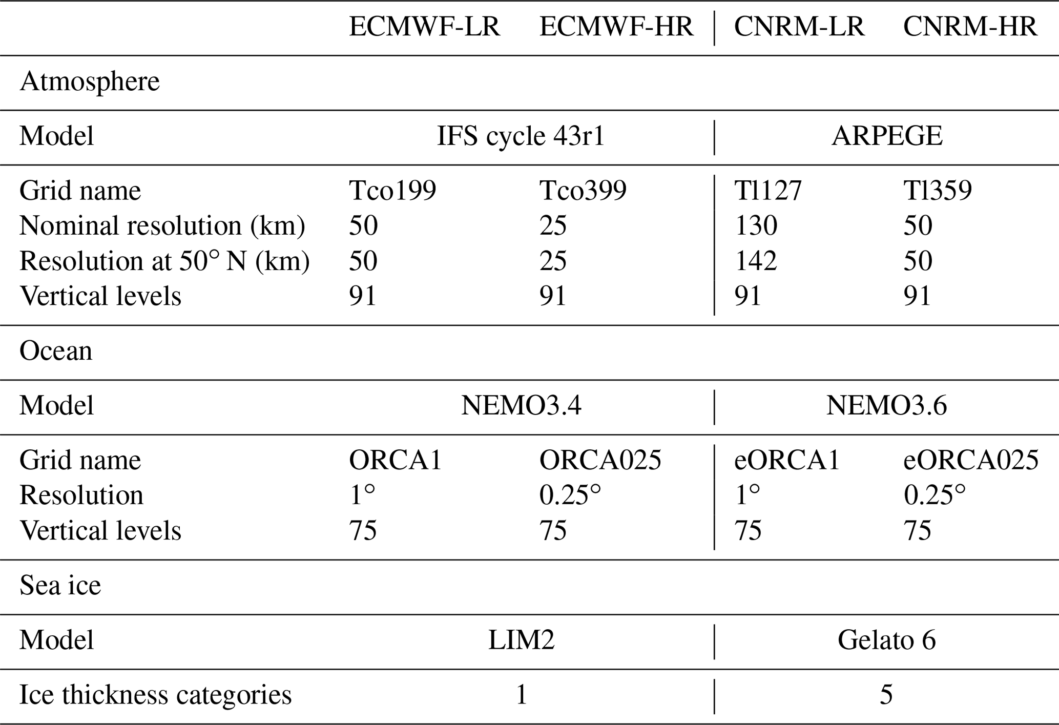
Two fully coupled atmosphere–land–sea-ice–ocean GCMs, namely, ECMWF-IFS and CNRM-CM6-1, are used in this study and described below. These models participated in the HighResMIP, which was an endorsed sub-project of the sixth phase of the Coupled Model Intercomparison Project (CMIP6; Eyring et al., 2016). The model characteristics for each resolution are given in Table 1.
Table 1Characteristics of the two models at two different resolutions used in this study.
2.1.1 ECMWF-IFS
The atmospheric component of ECMWF-IFS, the Integrated Forecasting System (IFS), uses a semi-implicit, semi-Lagrangian discretization (Ritchie et al., 1995; Temperton et al., 2001). The model is based on the IFS cycle 43r1. The land surface component is the Hydrology Tiled ECMWF Scheme of Surface Exchanges over Land (H-TESSEL; Balsamo et al., 2009). The ocean component is version 3.4 of the Nucleus for European Modelling of the Ocean (NEMO3.4; Madec et al., 2013). NEMO3.4 is coupled to the second version of the Louvain-la-Neuve Sea-Ice Model (LIM2; Bouillon et al., 2009; Fichefet and Morales Maqueda, 1997), which includes a three-layer model for the vertical conduction of heat in sea ice. The coupling between the ocean and atmosphere is resolved by the sequential single-executable strategy used by Mogensen et al. (2012) at a frequency of 1 h (Roberts et al., 2018b). There is no coupling between precipitation over land and the runoff to the ocean, but, to overcome this limitation, a climatological approximate calculation of the freshwater input is determined at each coastal grid point. Finally, unlike the operational setup of ECMWF, where the surface energy balance is calculated in the land surface module (Mogensen et al., 2012), the skin temperature from LIM2 is coupled to mitigate the excessive sea ice volume in the Arctic.
Two different configurations of the model have been used. The first configuration, ECMWF-IFS-LR (hereafter ECMWF-LR), uses the Tco199 grid for the atmosphere, which has a horizontal resolution of about 50 km, and the ORCA1 tripolar grid for the ocean, which has a nominal resolution of ∼ 1∘ (Roberts et al., 2018b). The second configuration, ECMWF-IFS-HR (hereafter ECMWF-HR), uses the Tco399 grid for the atmosphere, which has a horizontal resolution of about 25 km, and the ORCA025 tripolar grid for the ocean, which has a resolution of ∼0.25∘. The vertical resolution is the same for both configurations, with 91 levels in the atmosphere, extending up to 0.01 hPa, and 75 levels in the ocean (Madec, 2016). Beside the resolution, the only differences between the two configurations come from the resolution-dependent parameterizations in NEMO (Roberts et al., 2018b). Both configurations of the model simulate the Quasi-Biennial Oscillation (QBO) variability reasonably well (not shown).
2.1.2 CNRM-CM6-1
The atmospheric component of CNRM-CM6-1 is version 6.3 of the global atmospheric model ARPEGE‐Climat (Voldoire et al., 2019). It uses a semi‐Lagrangian numerical integration scheme and has 91 verticals levels with a high-top level at 0.01 hPa. The model is based on cycle 37 of the ARPEGE/IFS system. This model is coupled to the surface component SURFEX, which shares the same grid and time step (Masson et al., 2013). The ocean component is NEMO3.6 (Madec et al., 2017), which includes 75 vertical levels. The sea ice component is Gelato 6, which is embedded into the ocean component. Gelato 6 uses five ice thickness categories, in which each category treats the snow as a single layer, while ice is simulated with a nine‐layer vertical discretization (Voldoire et al., 2019). The coupling between the atmosphere and ocean–sea ice components is performed using the OASIS3‐MCT software (Craig et al., 2017) at a 1hr frequency.
The first configuration, CNRM-CM6-1 (hereafter CNRM-LR), uses the Tl127 grid for the atmosphere, which has a nominal horizontal resolution of 130 km, and the eORCA1 horizontal grid for the ocean (Table 1), which is an extension of the ORCA1 tripolar grid that differs from ORCA1 by the use of two quasi‐isotropic bipolar grids south of 67∘ S instead of the former Mercator grid (Voldoire et al., 2019). The second configuration, CNRM-CM6-1-HR (hereafter CNRM-HR), uses the Tl359 grid for the atmosphere, which has a nominal horizontal resolution of 50 km, and the eORCA025 horizontal grid for the ocean. The vertical resolutions are similar for both configurations and both components (atmosphere and ocean) and enable simulation of the QBO (Richter et al., 2020).
2.2 Experiments
Two different experiments are conducted with each model configuration and follow the protocol defined within the PRIMAVERA project. The first experiment, the control run (CTRL), has a constant forcing corresponding to the year 1950 and is run for 100 years without including 30 years of spin-up, which are not analyzed in this study. This control run is similar to the 1950 control simulation of HighResMIP (Haarsma et al., 2016). The second experiment, the perturbation run (PERT), has the same constant forcing as CTRL but with a modified sea ice albedo. In the PERT experiment, the sea ice albedo values (dry snow, melting snow, bare frozen ice and bare puddled ice) are reduced to the open-ocean value (∼0.07) from the first model time step (1 January) and are kept equal to this value through the whole model integration to achieve a large Arctic sea ice loss in summer. This perturbation increases the absorption of solar radiation and generates a melting of the snow over sea ice and of the sea ice itself. This method has already been applied in previous studies but on much longer timescales (Deser et al., 2015; Blackport and Kushner, 2016, 2017; Park et al., 2018) and produces consistent climate responses compared to other methods (Screen et al., 2018; Sun et al., 2020). The PERT experiment is run for 15 months only as our study focuses on the short-term climate response to Arctic sea ice loss. Moreover, in order to sample the internal climate variability, 40 members are performed in the PERT experiment, where each member starts from a different year of CTRL. This number of members was chosen because it allows a good level of statistical significance to be reached in several high-latitude regions, mainly in the surface air temperature response (Screen et al., 2014), without demanding too much computing time. One member is launched every year from CTRL with ECMWF-LR and ECMWF-HR, every 2 years with CNRM-HR, and every 3 years with CNRM-LR. As the difference between PERT and CTRL is only a change in sea ice, comparing them enables the isolation of the effect of sea ice loss. To perform our analysis, we compare each member of PERT to the member of its corresponding year in CTRL (PERT−CTRL). The atmospheric responses are scaled by the amount of Arctic sea ice extent loss averaged over the summer (July, August and September here). Finally, the statistical significance of the atmospheric response, shown on maps, has been estimated using a two-sample Kolmogorov–Smirnov test accounting for the false discovery rate (FDR) (Wilks, 2016). The FDR method was first described by Benjamini and Hochberg (1995) and limits spurious local test rejections. Indeed, the rejection of the null hypothesis is valid if the p values are not larger than a threshold level (10 %) that depends on the distribution of the sorted p values (Wilks, 2016) obtained here thanks to a two-sample Kolmogorov–Smirnov test.
2.3 Climate extreme indices
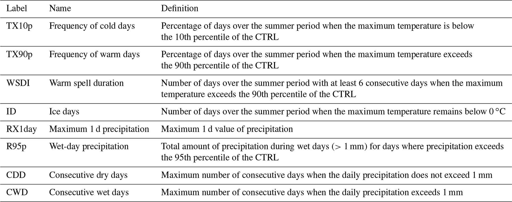
To determine the changes in extreme climate events, 27 climate extreme indices have been defined by the Expert Team on Climate Change Detection and Indices (ETCCDI) created by the World Climate Research Programme (WCRP). These indices are mainly used in historical climate model simulations (e.g. Sillmann et al., 2013a) and in model projections forced by greenhouse gas emission increases (Sillmann et al., 2013b). Eight climate extreme indices of the ETCCDI are used in this study and are summarized in Table 2. These indices are able to show extreme changes in surface air temperature and in precipitation over high-latitude regions because they use either a relative change based on a percentile or a threshold suitable for these regions, such as a threshold to 0 ∘C for the ice days index. Four indices are based on the maximum daily surface air temperature: the frequency of cold days (TX10p: percentage of days over the summer period when the maximum temperature is below the 10th percentile of the CTRL), the frequency of warm days (TX90p: percentage of days over the summer period when the maximum temperature exceeds the 90th percentile of the CTRL), the warm spell duration index (WSDI: number of days over the summer period with at least 6 consecutive days when the maximum temperature exceeds the 90th percentile of the CTRL) and the ice days (IDs: number of days over the summer period when the maximum temperature remains below 0 ∘C). This last index (ID) should not be confused with sea ice conditions. The last four indices are based on the daily precipitation: the maximum 1 d precipitation (RX1day: the maximum 1 d value of precipitation over the summer period), the wet-day precipitation (R95p: total amount of precipitation during wet days (>1 mm) for days where precipitation exceeds the 95th percentile of the CTRL over the summer period), the consecutive dry days (CDDs: maximum number of consecutive days over the summer period when the daily precipitation does not exceed 1 mm) and the consecutive wet days (CWDs: maximum number of consecutive days over the summer period when the daily precipitation exceeds 1 mm). More details are given below or can be found in Zhang et al. (2011) or in Sillmann et al. (2013a) for all the indices.
For each calendar day, the values of the 10th (for TX10p) and 90th percentiles (for TX90p and WSDI) of the 40-year period CTRL centered on a 5 d window are first calculated (the vertical blue lines in Fig. 1 on 1 August for example). For each month, the number of days exceeding the 90th percentile or less than the 10th percentile is calculated in PERT and in CTRL and finally weighted by the number of calendar days in this same month (divided by 31 d in August for instance). Finally, the difference between the percentage of days in a month exceeding the threshold in PERT and in CTRL is computed. The other indices are also determined for CTRL and PERT to be able to compare both simulations and to understand the effect of sea ice loss on the extremes.
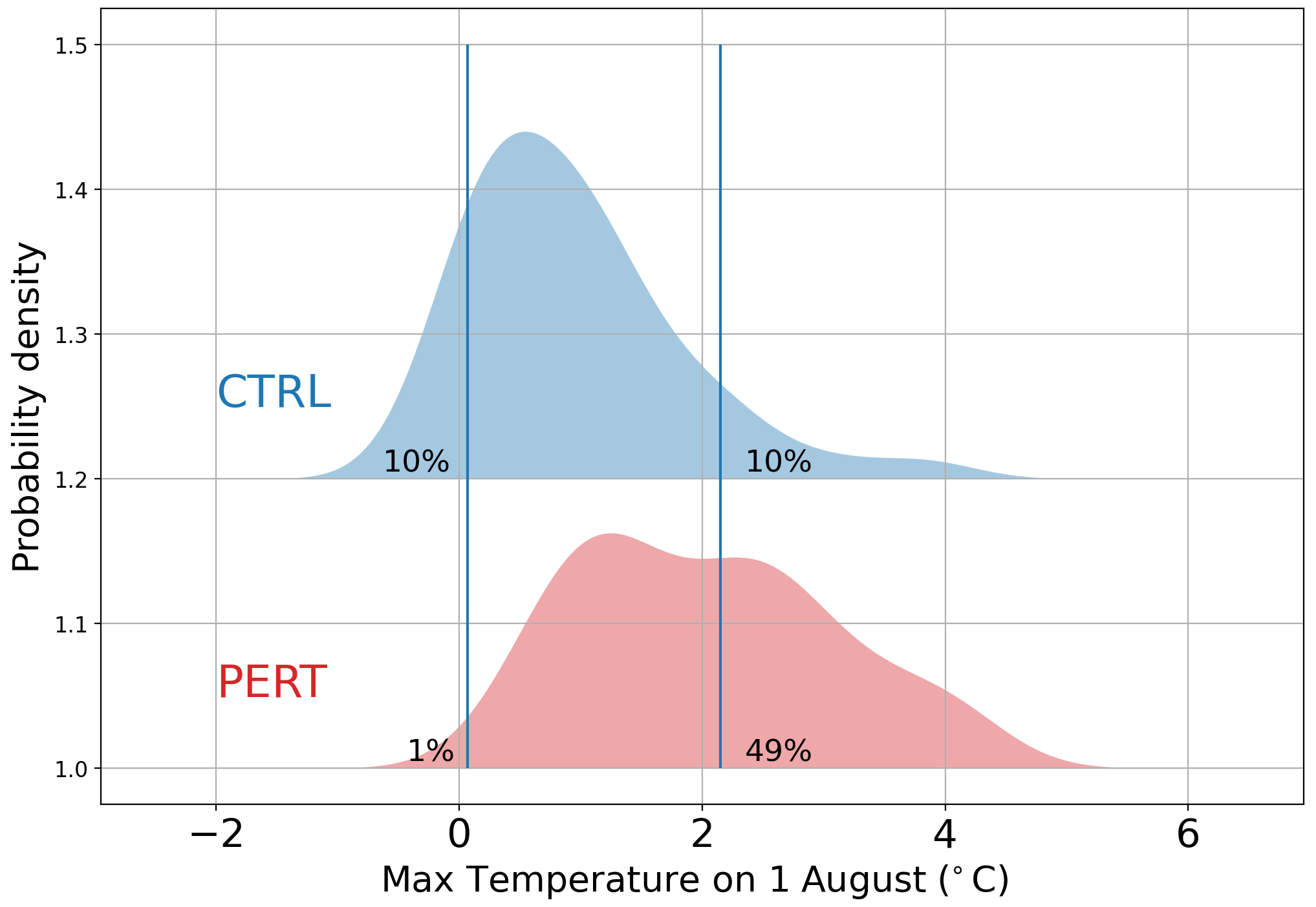
Figure 1Probability density function of the maximum surface air temperature over Svalbard in CTRL (blue) and in PERT (red) on 1 August. The left and right vertical blue lines show the 10th and 90th percentiles of the CTRL on a 5 d window, respectively. The percentage next to the vertical lines indicates the frequency of days exceeding the 10th (left) and the 90th (right) percentiles of the CTRL.
2.4 Studied areas
Different Arctic regions are considered according to the definitions given in Table 3, and only the continental grids (land area) of each region are used in this study. The eight climate extreme indices are first determined for each grid cell, then the regional average is computed. Note that when performing spatial averaging, the latitudinal variation in grid cell area is taken into account by weighting the values by the cosine of the latitude. There is no longitudinal variation in grid cell area.
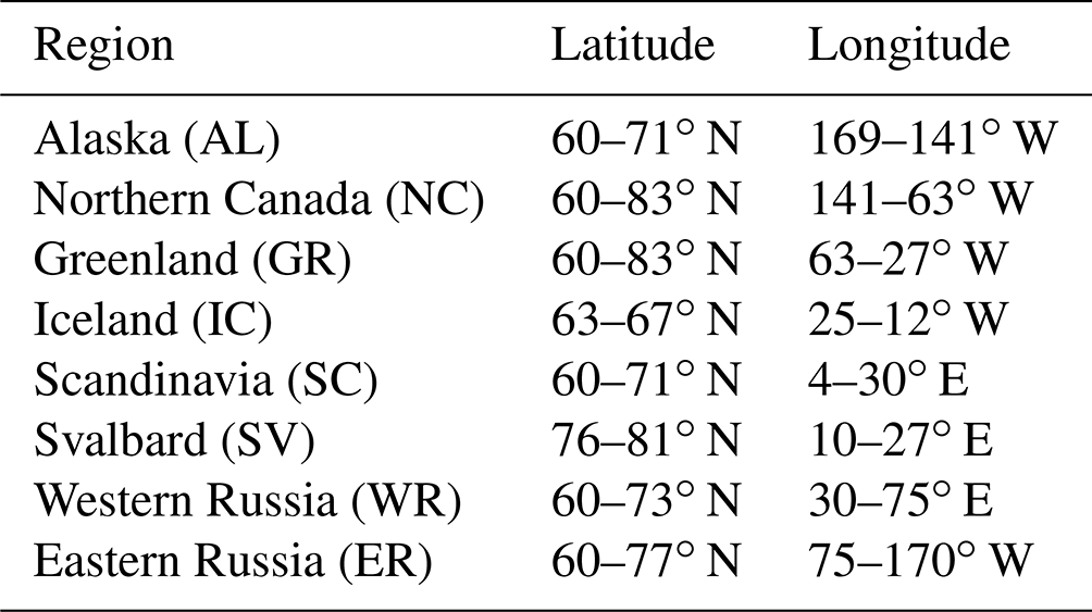
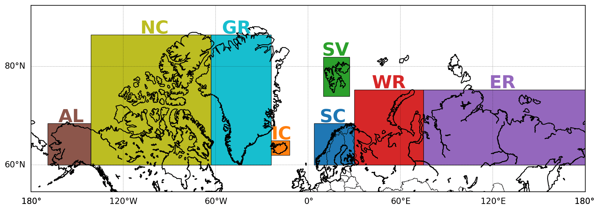
Figure 2Regions considered in this study. AL stands for Alaska, NC for northern Canada, GR for Greenland, IC for Iceland, SC for Scandinavia, SV for Svalbard, WR for western Russia and ER for eastern Russia.
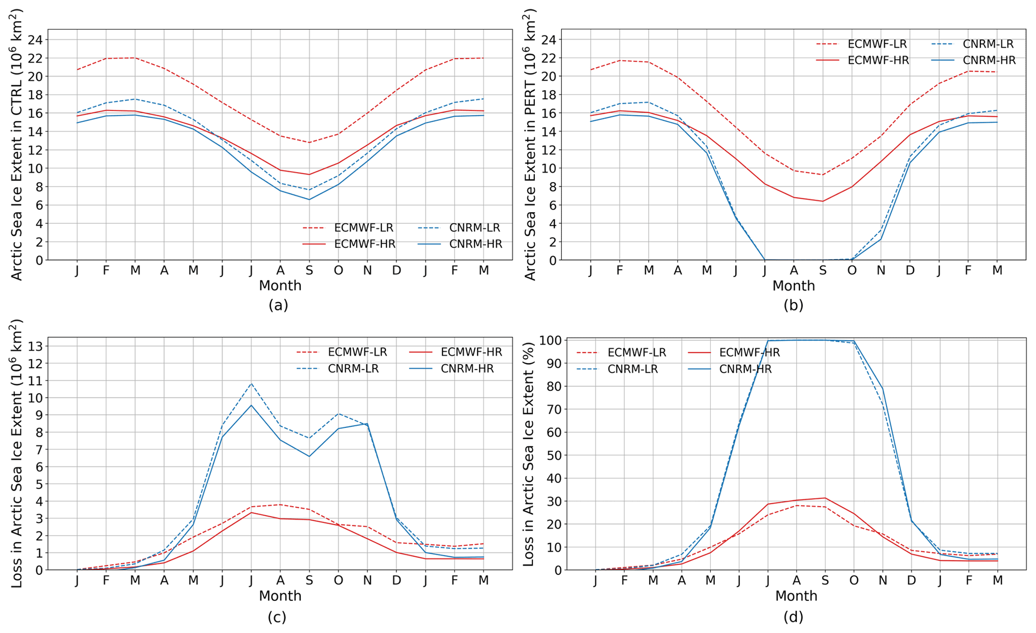
Figure 3Arctic sea ice extent (in millions of square kilometers) in CTRL (a) and in PERT (b). Panels (c) and (d) show the decrease in Arctic sea ice extent in PERT compared to CTRL (i.e. CTRL−PERT) in millions of square meters and in percent relative to the CTRL value, respectively.
3.1 Sea ice loss
The seasonality of Arctic sea ice extent in CTRL is well represented for all models, with a minimum in September and a maximum in February/March (Fig. 3). However, sea ice extent is overestimated throughout the year in ECMWF-LR, while it fits well with the 1950s observations with a sea ice extent around 16×106 and 8×10⁶ km2 in March and September, respectively (e.g. Walsh et al., 2017), in the other models. The prescribed drastic change in sea ice albedo (PERT) induces a significant reduction in Arctic sea ice extent, peaking in summer (Figs. 3 and 4). The sea ice loss in PERT is especially unrealistic in CNRM. Note that using the albedo reduction technique underestimates the sea ice loss in winter and thus impacts the magnitude of the climate responses (Sun et al., 2020). Nonetheless, a good consistency in these responses among different techniques to impose sea ice reductions has been observed (Sun et al., 2020). Moreover, the albedo reduction technique estimates the sea ice loss well during summer, the season studied here, compared to other techniques (Sun et al., 2020).
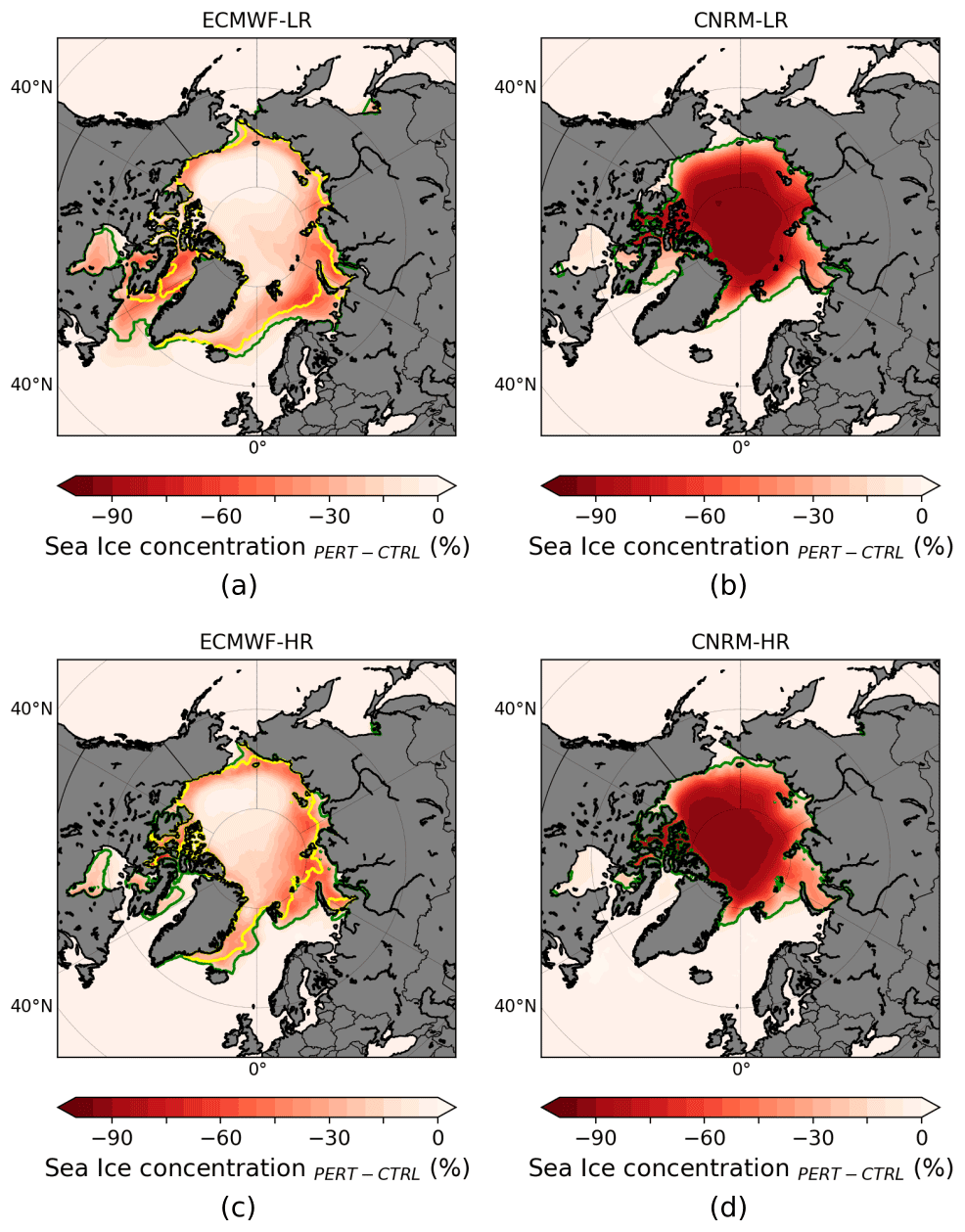
Figure 4Arctic sea ice concentration change (PERT−CTRL) in summer (JAS) in ECMWF-LR (a) and CNRM-LR (b). (c–d) As (a)–(b) but for models at high resolution. The green and yellow lines show the sea ice edge (15 % ice concentration) from CTRL and PERT, respectively. Note that for the two CNRM model configurations, no yellow line is present because the sea ice has disappeared in PERT.
The induced sea ice loss in these experiments depends on the model used, although the experimental setup is the same. The decrease in summer Arctic sea ice extent in PERT compared to CTRL reaches 30 % for the two ECMWF model configurations and is largely localized in the Barents and Kara seas and in the eastern Arctic. In the CNRM models, it reaches up to 100 %, and it is associated with a total disappearance of sea ice (Figs. 3d and 4). These discrepancies may arise due to a significant difference in mean sea ice state between the models, with a large mean sea ice thickness in the ECMWF configurations (Figs. A1 and A2), which is closer to reanalysis estimates (Zhang and Rothrock, 2003) than CNRM, and relatively low ocean heat transport (Roberts et al., 2018b; Docquier et al., 2019), which could lead to more sea ice being retained in PERT in ECMWF.
The sea ice loss also depends on the horizontal resolution, albeit weakly. More absolute sea ice loss is indeed simulated in the low-resolution models (Fig. 3c). This might be due to larger Arctic sea ice extent in CTRL at lower resolution, particularly in the Atlantic sector of the Arctic Ocean (Figs. 3a and 4). A higher ocean resolution generally leads to a decrease in sea ice extent and volume in CTRL in several GCMs used in the PRIMAVERA project due to enhanced poleward oceanic heat transport (Docquier et al., 2019).
3.2 Temperature extremes
The impact of Arctic sea ice loss on the maximum surface air temperature is now analyzed. Figure 5 shows the response of maximum daily surface air temperature per 1×10⁶ km2 of sea ice loss in summer (JAS). As expected, an increase in maximum daily temperature is found over the Arctic. The warming extends to surrounding landmasses such as Canada, Scandinavia and northern Russia. Over high latitudes, the CNRM response is larger than the ECMWF one, even after scaling the response by the amount of sea ice loss. This could be explained by the insulating effect of sea ice in ECMWF, which still simulates more than 2 m thick sea ice in PERT in summer (Fig. A1b) and can limit the warming in that model. The change in horizontal resolution does not strongly impact the response, as observed in Streffing et al. (2021), except over the southern Labrador Sea in ECMWF. In this model, sea ice is present in that area in CTRL at low resolution but not at high resolution, leading to a warming in ECMWF-LR that is nearly absent in ECMWF-HR.
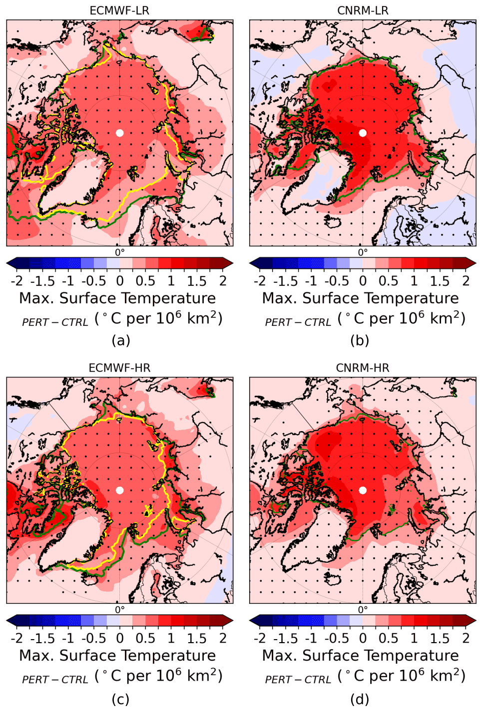
Figure 5Ensemble mean changes (PERT−CTRL) in maximum daily surface air temperature response over the entire summer (JAS) scaled by the amount of sea ice extent loss for ECMWF-LR (a), CNRM-LR (b), ECMWF-HR (c) and CNRM-HR (d). The dots show where the response is statistically significant according to a 10 % level FDR test associated with a Kolmogorov–Smirnov test. The green and yellow lines represent the sea ice edge (15 % ice concentration) from CTRL and PERT, respectively.
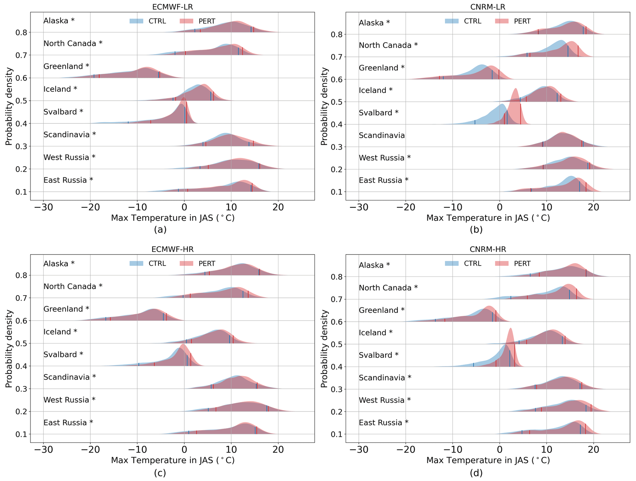
Figure 6Probability density function (PDF) of the daily maximum surface air temperature (∘C−1) in summer (JAS) for ECMWF-LR (a), CNRM-LR (b), ECMWF-HR (c) and CNRM-HR (d). PDF of the CTRL is the blue distribution, and PDF of the PERT is the red distribution. The left blue (red) line and the right blue (red) line correspond to the 10th percentile and 90th percentile of the CTRL (PERT), respectively. A star next to the name of the region shows if the distribution change is statistically significant according to a 5 % level Kolmogorov–Smirnov test. An offset on the y axis of 0.1 is taken into account for each region.
The probability density function (PDF) of the daily summer maximum temperature is shown in Fig. 6 for eight different peripheral Arctic regions (defined in Table 3 and Fig. 2). The change in PERT compared to CTRL is stronger in CNRM (Fig. 6) because the response cannot be scaled by the amount of sea ice loss in this figure, and CNRM experiences a larger Arctic sea ice loss than ECMWF (Figs. 3 and 4). A shift to the right of the PDF in PERT compared to CTRL, going hand in hand with a shift in the mean towards higher values, occurs due to sea ice loss over all the selected regions. Nonetheless, this shift is not symmetrical for most regions, with a larger shift in the left part of the distribution (low temperatures) compared to the right part (high temperatures), leading to a change in the shape of the distribution. This means that low maximum surface air temperatures increase more than high maximum surface air temperatures, in agreement with previous studies focusing on high latitudes (Kharin et al., 2013; Sillmann et al., 2013a).
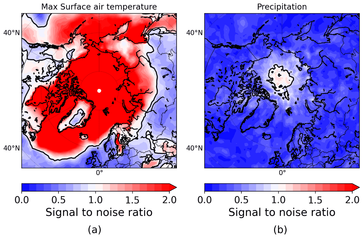
Figure 7Signal-to-noise ratio in summer averaged for all the models for the daily maximum surface air temperature (a) and for the daily precipitation (b) responses to summer Arctic sea ice loss. The black line represents where the signal-to-noise ratio is equal to 1.
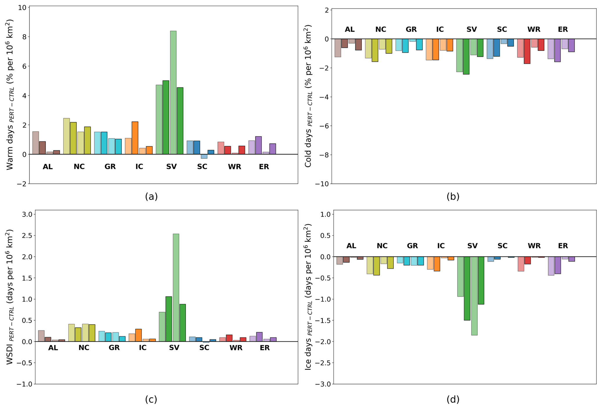
Figure 8Ensemble mean changes (PERT−CTRL) per month averaged in summer (JAS) in warm days (a), cold days (b), warm spell duration index (c) and ice days (d) scaled by the amount of sea ice extent loss for the eight regions defined in Table 3 (Fig. 2) for ECMWF-LR (left light bar), ECMWF-HR (left dark bar), CNRM-LR (right light bar) and CNRM-HR (right dark bar).
Furthermore, the magnitude of the warming depends on the region. The warming over Svalbard is obviously stronger than in other regions as Svalbard is made up of islands surrounded (at least in part) by sea ice in early summer in all models in CTRL. Thus, the sea ice loss in PERT impacts this region more easily than a continent or an island further south such as Iceland. Northern Canada, which is composed of hundreds of islands surrounded by sea ice, is the region with the second-strongest warming. Greenland, although it is an island partially surrounded by sea ice, experiences less warming than the two last regions because an ice sheet covers almost the whole island, and temperatures are much lower over central Greenland, where the altitude is high, than over other Arctic regions, which does not lead to an important melt of the sea ice and could mitigate the maximum surface air temperature response to a sudden sea ice loss over that region (Figs. 5 and 6). The warming over Greenland and northern Canada can be related to a negative change in the North Atlantic Oscillation (NAO) (Folland et al., 2009; Ding et al., 2014). However, in these experiments, only CNRM-LR displays a negative change in the NAO, but this change is small compared to the variability in the ensemble (Fig. A3). As this index exhibits a high variability, 40 members (and even 80 members by combining the two resolutions) are not enough to detect a robust response in the NAO index.
The increase in maximum surface air temperature over the peripheral Arctic regions is robust, although a large internal climate variability is present. The signal-to-noise ratio, estimated as the ensemble mean response divided by the standard error, reveals that the signal exceeds the noise due to internal climate variability over the vast majority of high-latitude regions (Fig. 7a). However, in some regions such as western Scandinavia, the center of Greenland, the Northwest Territories of Canada and the regions of Russia close to 60∘ N, the noise exceeds the signal, showing that the response is small compared to the role of internal climate variability even in regions relatively close to the sea ice front.
Figure 8 shows four different temperature extreme indices (see Sect. 2.3) for the eight different regions in summer. As expected, all regions experience an increase in frequency of warm days (Fig. 8a), a decrease in frequency of cold days (Fig. 8b), an increase in warm spell duration (Fig. 8c) and a decrease in the number of ice days (Fig. 8d) due to Arctic sea ice loss. Svalbard exhibits a more drastic change compared to other regions. Indeed, an absolute increase of around 5 % (up to 8 % in CNRM-LR) in warm-day frequency (Fig. 8a) and also of around 1 d per month (up to 2.5 d per month in CNRM-LR) in warm spell duration (Fig. 8c) per 1×10⁶ km2 of sea ice loss is simulated over this region. Furthermore, a loss of 1×10⁶ km2 of sea ice leads to a reduction of at least 1 ice day per month in Svalbard (Fig. 8d). Other regions experience less intense change in frequency or persistence, but all models agree on the sign of the change except over Scandinavia. These results cannot be directly compared to those of the idealized atmospheric general circulation model simulations forced by projected Arctic sea ice loss of Screen et al. (2015) because, in the latter study, the response is not scaled by the amount of sea ice loss, the oceanic areas are taken into account, and the response is averaged over an entire year. However, a global Arctic sea ice loss does not seem to lead to the recent increase in heat waves that happened almost only over north-eastern Canada and Greenland (Dobricic et al., 2020).
The maximum daily surface air temperature increase is larger in autumn than in summer (not shown), even if the sea ice loss is smaller in autumn (see Fig. 3). This can be explained by the turbulent heat flux response, which is enhanced in autumn due to a large contrast between the air and surface temperatures during this season (e.g. Deser et al., 2010). However, the increase in frequency of warm days and in the warm spell duration is larger in summer over peripheral Arctic regions (not shown), highlighting the usefulness of studying the response of extreme events during this season. Finally, all extreme indices studied here show a significant increase mainly localized over the Arctic Ocean, which hardly extends over continents (e.g. Fig. A4). Nonetheless, the change in frequency of extremes (warm days and cold days) extends more easily towards continents than the change in persistence of extremes (WSDI).
3.3 Precipitation extremes
We now investigate the precipitation response with Fig. 9, which shows the monthly mean precipitation response to sea ice loss in summer. An increase in precipitation is found over the Arctic, which is only statistically significant in CNRM. Newly open waters lead to an increase in evaporation, resulting in enhanced precipitation there, in agreement with previous studies (e.g. Deser et al., 2010; Semmler et al., 2012; Bintanja and Selten, 2014; Semmler et al., 2016; Smith et al., 2017; England et al., 2018). However, although little sea ice melts in PERT over the central Arctic in summer in ECMWF, an increase in precipitation, not statistically significant, is simulated over this region (Fig. 9a, c). The fact that this response is not statistically significant shows the small signal and the greater importance of internal climate variability for this variable compared to surface air temperature (Screen et al., 2014). Indeed, only the region close to the North Pole experiences a signal larger than the noise for the precipitation response (Fig. 7b); elsewhere, the response is weak compared to internal variability. Furthermore, even by combining the two resolutions (and having 80 members), the precipitation response is still not statistically significant in peripheral Arctic regions (not shown).
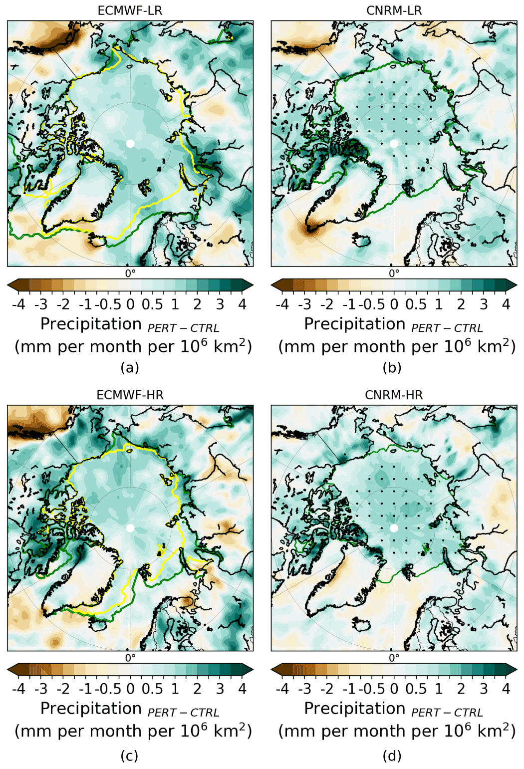
Figure 9Ensemble mean changes (PERT−CTRL) in summer (JAS) precipitation scaled by the amount of sea ice extent loss for ECMWF-LR (a), CNRM-LR (b), ECMWF-HR (c) and CNRM-HR (d). The dots show where the response is statistically significant according to a 10 % level FDR test associated with a Kolmogorov–Smirnov test. The green and yellow lines represent the sea ice edge (15 % ice concentration) from CTRL and PERT, respectively.
No significant change in net precipitation (P–E) is observed over the central Arctic (Fig. A5), showing that the increase in precipitation is balanced by the increase in local evaporation over that region. However, a decrease in P–E is detected near the continental edges of the Arctic Ocean, which is statistically significant in CNRM (Fig. A5b, d). This highlights the fact that the increase in evaporation is larger than the increase in precipitation, which leads to an increase in ocean surface salinity (not shown) despite the melting sea ice in these areas.
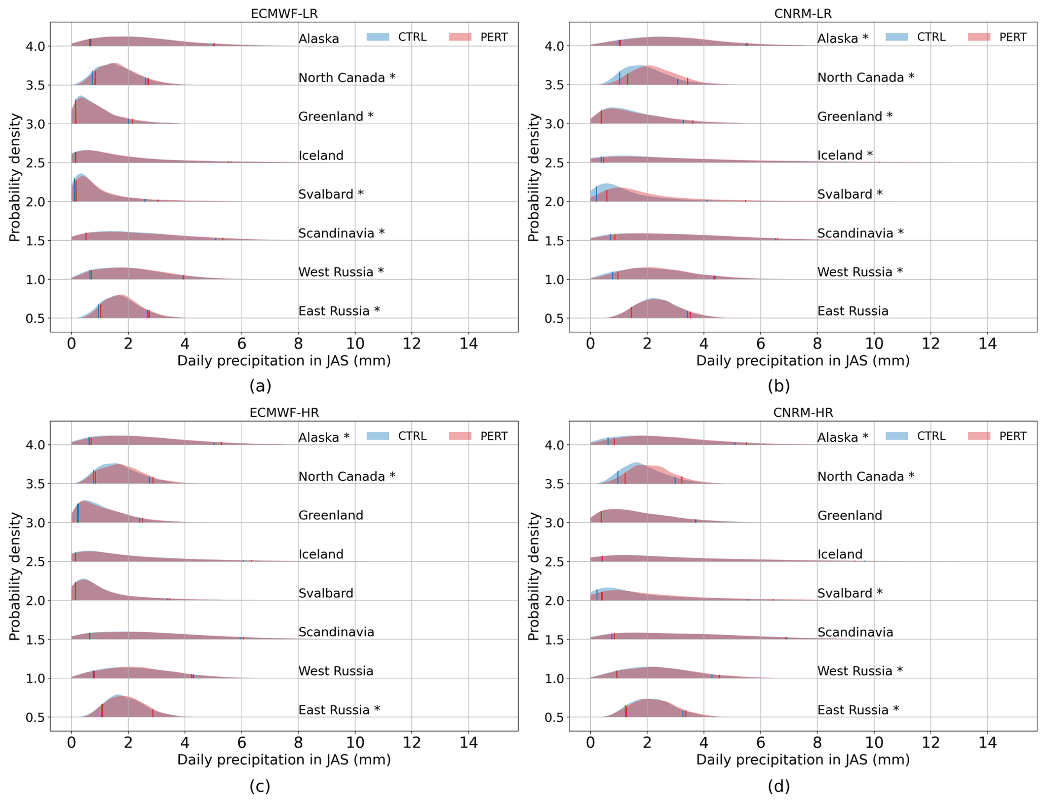
Figure 10PDF of the daily precipitation in summer (JAS) for ECMWF-LR (a), CNRM-LR (b), ECMWF-HR (c) and CNRM-HR (d). PDF of the CTRL is the blue distribution, and PDF of the PERT is the red distribution. The left blue (red) line and the right blue (red) line correspond to the 10th percentile and 90th percentile of the CTRL (PERT), respectively. A star next to the name of the region shows if the distribution change is statistically significant according to a 5 % level Kolmogorov–Smirnov test. An offset on the y axis of 0.1 is taken into account for each region.
The PDF of the daily precipitation in summer is shown in Fig. 10. A shift to the right of the PDF in PERT, reflecting an increase in precipitation, occurs in some regions due to sea ice loss. Nonetheless, the shift is weaker in the daily precipitation response (Fig. 10) than in the daily maximum surface air temperature response (Fig. 6). The change in the distribution between CTRL and PERT seems to be symmetrical in all regions except in Svalbard in CNRM. As for the maximum surface air temperature (Fig. 6), the shift is larger in CNRM due to the greater loss of sea ice (Fig. 10), leading to a greater surface heat flux change in this model than in ECMWF (not shown), and can explain the larger response in precipitation in CNRM. Moreover, the increase in precipitation is also stronger in Svalbard and in northern Canada because these regions are made up of islands surrounded by sea ice, which melts in PERT. Newly open waters are observed in these regions and lead to a significant increase in precipitation. Furthermore, surface waters are warmer in PERT and generate more evaporation. Finally, as the surface air temperature increases in PERT, the water vapor content increases and can therefore potentially generate more precipitation. In all other regions, the shift to the right of the precipitation distribution is rather weak (Fig. 10). If we now compare the resolutions, no significant differences occur between the LR and the HR, as reported in Streffing et al. (2021).

Figure 11Ensemble mean changes (PERT−CTRL) per month in summer (JAS) in maximum 1 d precipitation (a), very wet days (b), consecutive dry days (c) and consecutive wet days (d) scaled by the amount of sea ice extent loss for the eight regions (Fig. 2) for ECMWF-LR (left light bar), ECMWF-HR (left dark bar), CNRM-LR (right light bar) and CNRM-HR (right dark bar). The response is scaled by the amount of the summer Arctic sea ice loss.
Figure 11 shows four different precipitation extreme indices (see Sect. 2.3) for the regions in the peripheral Arctic in summer. An increase in the intensity of precipitation extreme is simulated in all regions (Fig. 11a, b) and supports the recent observed (Chernokulsky et al., 2019) and projected (Kharin et al., 2018) increase in heavy precipitation. If we average all the models, Svalbard is still the region with the largest increase in intensity of precipitation (Fig. 11a, b). However, other regions further south, such as Iceland or Scandinavia, experience an increase in intensity, which can be larger than in Svalbard in some models when the very wet days in a month are summed up (Fig. 11b). Regions over Russia display less significant changes, mainly in the maximum 1 d precipitation indices (Fig. 11a).
The change in persistence of extreme precipitation over the different regions (Fig. 11c, d), mainly in consecutive dry days (Fig. 11c), is not as consistent as the change in magnitude (Fig. 11a, b). Several regions, such as Greenland, Iceland, Scandinavia and western Russia, have a different sign in the response in the consecutive-dry-day duration to sea ice loss (Fig. 11c). In the other regions, all models show a decrease in the number of consecutive dry days. Nonetheless, the change in consecutive-wet-day duration is more consistent among the regions and the models (Fig. 11d). Over Greenland, a larger change in magnitude than in persistence of extreme precipitation is simulated and could be related to the lack of a significant circulation change (e.g. Fig. A3). Over Svalbard, a decrease in consecutive-dry-day duration and an increase in consecutive-wet-day duration of up to 0.3 d per 1×10⁶ km2 of sea ice loss are modeled in CNRM-LR (Fig. 11c, d) but are weaker in the other models. Finally, the response in persistence of extreme precipitation remains more restricted to the Arctic Ocean (Fig. 12) than the response in monthly mean precipitation (Fig. 9).
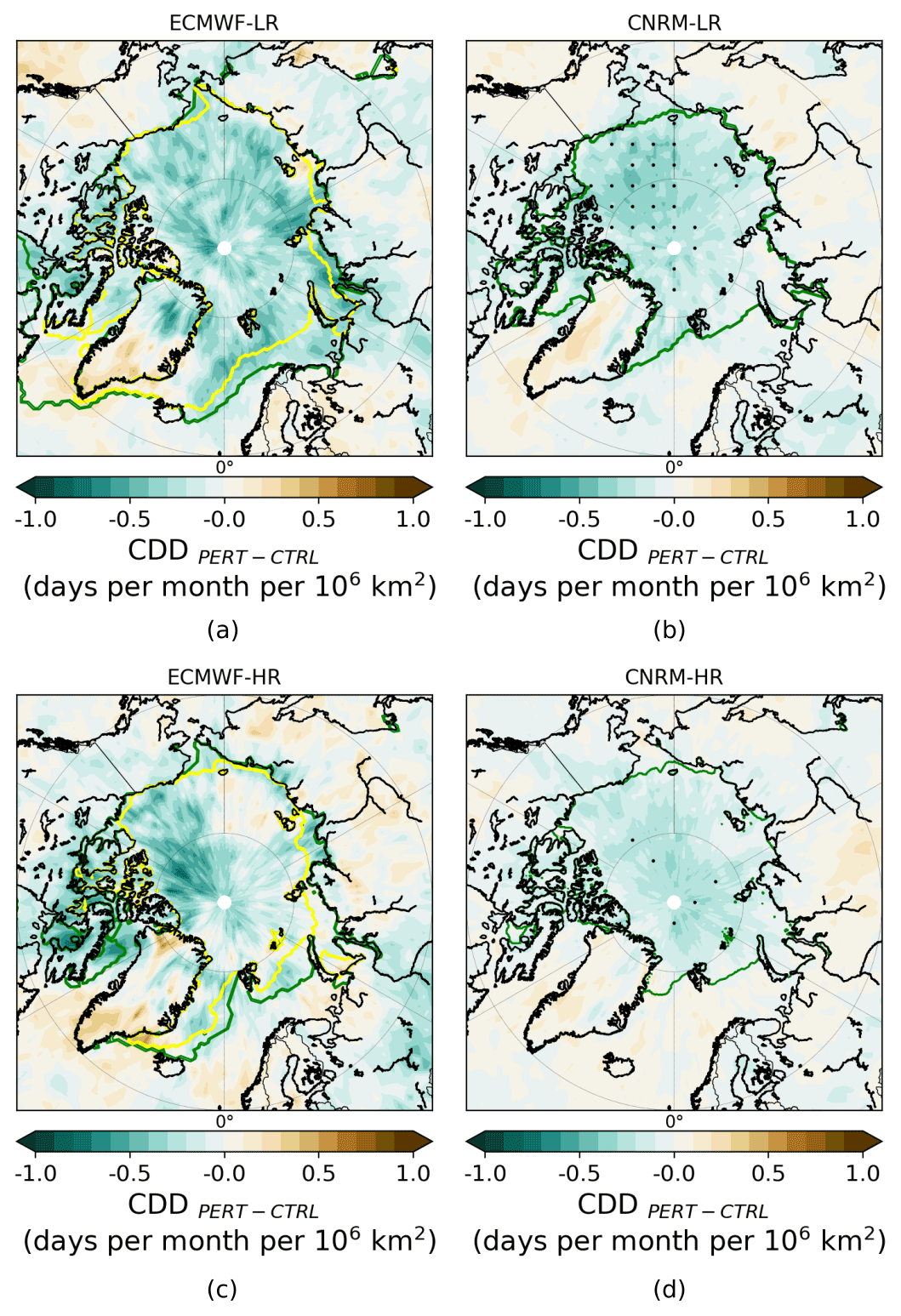
Figure 12Ensemble mean changes (PERT−CTRL) in summer (JAS) consecutive-dry-day duration scaled by the amount of sea ice extent loss in ECMWF-LR (a), CNRM-LR (b), ECMWF-HR (c) and CNRM-HR (d). The dots show where the response is statistically significant according to a 10 % level FDR test associated with a Kolmogorov–Smirnov test. The green and yellow lines represent the sea ice edge (15 % ice concentration) for CTRL and PERT, respectively.
As the Arctic sea ice continues its decline throughout the century, its variability is projected to increase (e.g. Goosse et al., 2009). Observing a drastic summer sea ice retreat for one particular year becomes a distinct possibility, yet the consequences of such an event on the atmosphere have been little explored. The summertime changes in temperature and precipitation extremes over the peripheral Arctic regions after a sudden sea ice retreat were investigated here. To our knowledge, this study is the first one to address this last question in depth following a coordinated (fully coupled) two-model approach in which idealized albedo experiments have been conducted. These experiments help to isolate as much as possible the effect of the Arctic sea ice loss without confounding factors, such as a change in sea surface temperature or in radiative forcing.
During the summer with a strong decline in Arctic sea ice extent, an increase in frequency and persistence of the maximum surface air temperature occurs over all the peripheral Arctic regions. This increase is especially large in regions made up of islands surrounded by sea ice in CTRL such as Svalbard or northern Canada. Svalbard experiences the largest change, with an increase of more than 4 % (per 1×10⁶ km2 of sea ice loss) in the frequency of warm days and of around 1 d (per 1×10⁶ km2 of sea ice loss) in warm spell duration index. Over all regions, the low maximum temperatures increase more than the high maximum temperatures in summer in response to sea ice loss.
An increase in extreme precipitation is also found over the peripheral Arctic regions. Nonetheless, the change in precipitation is smaller and less significant than the change in maximum surface air temperature. Furthermore, the response in extreme precipitation remains more restricted to the Arctic Ocean than the response in mean precipitation. Consistent with the temperature response, Svalbard shows again the largest change, with a decrease in consecutive-dry-day duration and an increase in consecutive-wet-day duration of 0.3 d (per 1×10⁶ km2 of sea ice loss) in CNRM-LR. However, an increase in the magnitude of precipitation occurs in all the peripheral Arctic regions in all models.
The increase in extreme precipitation is found in all the peripheral regions but is relatively small compared to internal climate variability. For the maximum surface air temperature, the signal exceeds the noise in the majority of the regions north of 60∘ N. Even if the two models (ECMWF and CNRM) experience different Arctic sea ice loss, both show a relatively similar change (scaled by the amount of sea ice loss) in maximum surface air temperature and precipitation, suggesting that the response over the peripheral Arctic regions evolves about linearly with respect to the amount of sea ice loss. This shows the minor importance of the role of the dynamical response in high latitudes, which tends to be non-linear (Petoukhov and Semenov, 2010), compared to the role of the thermodynamical response in summer. However, a stronger sea ice loss could produce a larger statistically significant response even when the response is scaled by the amount of sea ice loss. Finally, using a higher horizontal resolution does not considerably affect the response of extreme maximum surface temperature or precipitation.
Further studies are encouraged to study the response of climate extremes over Arctic regions to sudden sea ice loss as it can influence local communities (Ford et al., 2008), agriculture (Stevenson et al., 2014) and biodiversity (Hollowed et al., 2013; Haug et al., 2017). More members would be needed to detect robust change in extreme precipitation even at high latitudes. Moreover, it would be interesting to analyze the change in extremes over peripheral Arctic regions in summer with other sensitivity experiments simulating a more realistic seasonal cycle of Arctic sea ice loss and using different sea ice perturbation techniques, such as nudging. In conclusion, it is clear that Arctic sea ice loss alone impacts the extreme events of maximum surface temperature over the peripheral Arctic regions, and efforts such as those previously mentioned would help better quantify these climate impacts on these regions.
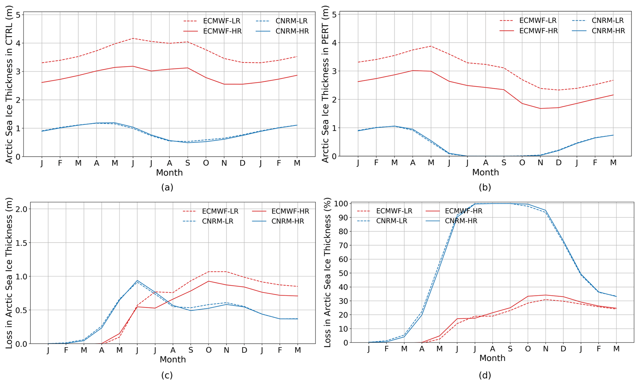
Figure A1Arctic sea ice thickness (in meters) in CTRL (a) and in PERT (b). Panels (c) and (d) show the decrease in Arctic sea ice extent in PERT compared to CTRL (i.e. CTRL−PERT) in meters and in percent relative to the CTRL value, respectively.
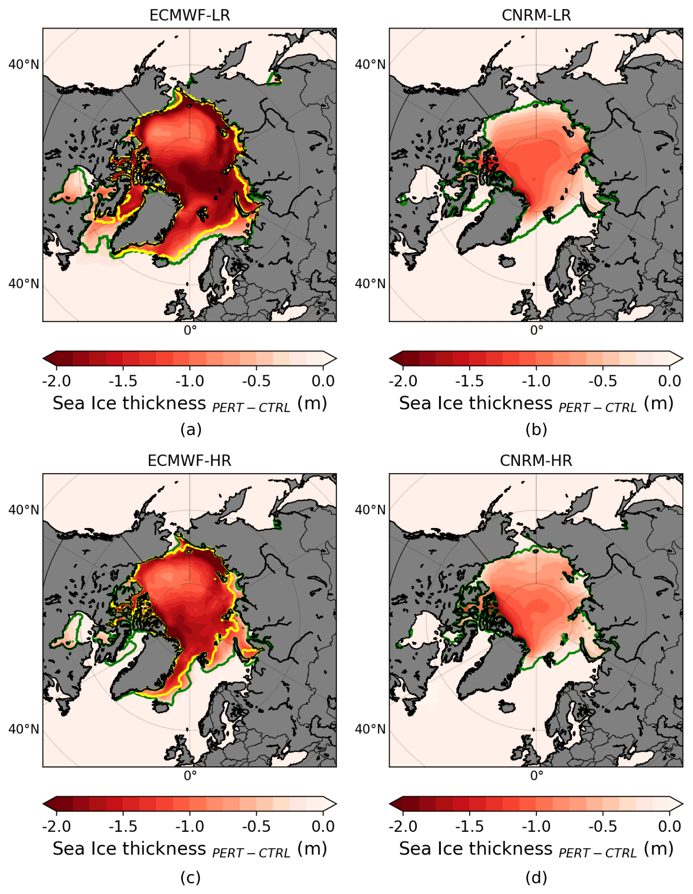
Figure A2Arctic sea ice thickness change (PERT−CTRL) in summer (JAS) in ECMWF-LR (a) and CNRM-LR (b). (c–d) As (a)–(b) but for models at high resolution. The green and yellow lines show the sea ice edge (15 % ice concentration) from CTRL and PERT, respectively. Note that for the two CNRM model configurations, no yellow line is present because the sea ice has disappeared in PERT.

Figure A3Boxplot of the summer NAO index (station-based method) in PERT compared to CTRL, where the CTRL has been taken as the 40-year reference period, for all members in each model. The p value of a Kolmogorov–Smirnov test between PERT and CTRL is shown below each boxplot.

Figure A4Ensemble mean changes (PERT−CTRL) in summer (JAS) warm spell duration index scaled by the amount of sea ice extent loss in ECMWF-LR (a), CNRM-LR (b), ECMWF-HR (c) and CNRM-HR (d). The dots show where the response is statistically significant according to a 10 % level FDR test associated with a Kolmogorov–Smirnov test. The green and yellow lines represent the sea ice edge (15 % ice concentration) from CTRL and PERT, respectively.
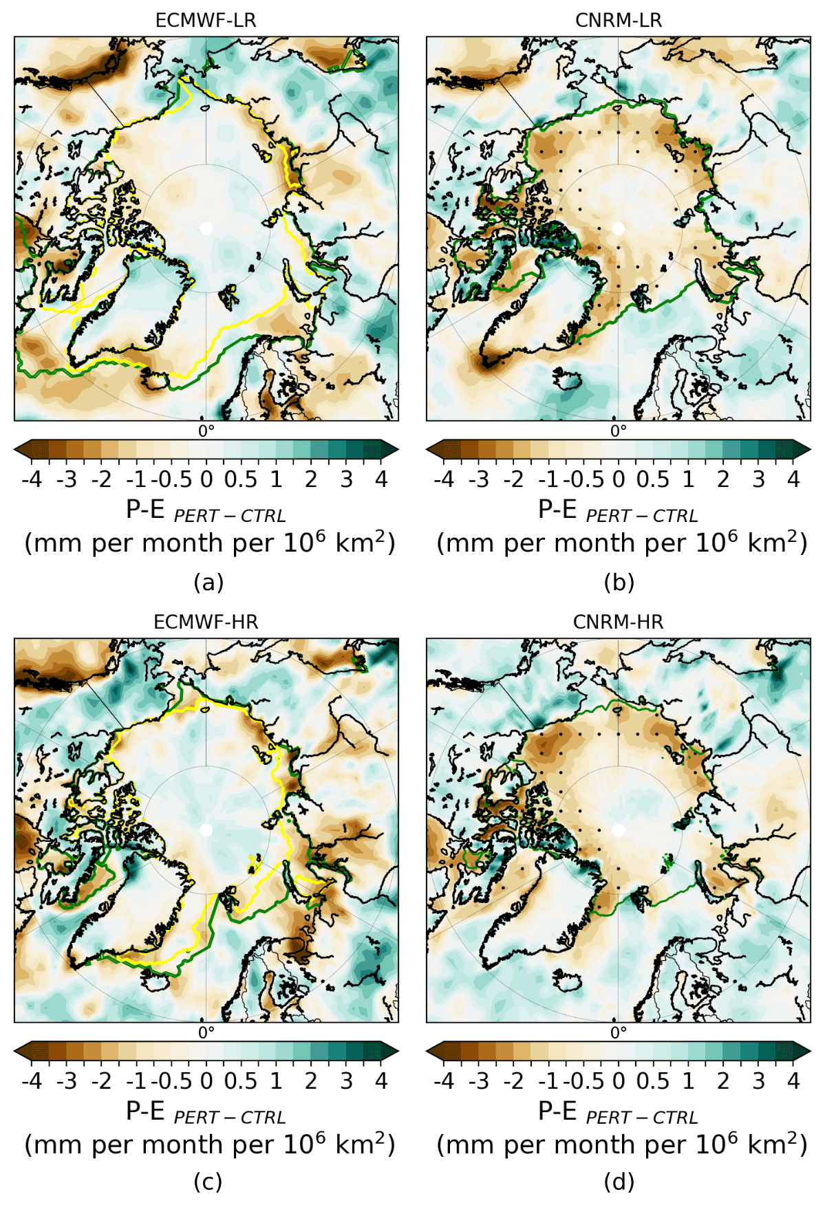
Figure A5Ensemble mean changes (PERT−CTRL) in summer (JAS) precipitation minus evaporation (P–E) scaled by the amount of sea ice extent loss for ECMWF-LR (a), CNRM-LR (b), ECMWF-HR (c) and CNRM-HR (d). The dots show where the response is statistically significant according to a 10 % level FDR test associated with a Kolmogorov–Smirnov test. The green and yellow lines represent the sea ice edge (15 % ice concentration) from CTRL and PERT, respectively.
The data from the CNRM model are openly available and can be shared upon request. The CTRL for the LR (https://doi.org/10.22033/ESGF/CMIP6.4946; Roberts et al., 2018a) and the HR (https://doi.org/10.22033/ESGF/CMIP6.4945; Roberts et al., 2017) are in the Earth System Grid Federation (ESGF) portal. The albedo experiments can be found in the Meteorological Archival and Retrieval System (MARS): https://doi.org/10.21957/h81p-dy58, ECMWF, 2022c; https://doi.org/10.21957/wtfp-4p86, ECMWF, 2022d; https://doi.org/10.21957/nddk-7k86, ECMWF, 2022a; https://doi.org/10.21957/war5-0281, ECMWF, 2022b.
SD, TF, FM, DD and RM conceptualized the science plan. RM, SC, CR, SK and RS conducted the experiments. SD performed the analyses, produced the figures and wrote the manuscript based on the insights from the co-authors.
The contact author has declared that neither they nor their co-authors have any competing interests.
Publisher’s note: Copernicus Publications remains neutral with regard to jurisdictional claims in published maps and institutional affiliations.
Steve Delhaye is a F.R.S–FNRS research fellow, Belgium (grant no. 1.A119.20). François Massonnet is a F.R.S.–FNRS research associate. Computational resources have been provided by the supercomputing facilities of the Université catholique de Louvain (CISM/UCL) and the Consortium des Équipements de Calcul Intensif en Fédération Wallonie Bruxelles (CÉCI) funded by the Fond de la Recherche Scientifique de Belgique (F.R.S.–FNRS) under convention 2.5020.11. David Docquier is supported by the JPI-Climate/JPI-Oceans ROADMAP project (Role of ocean dynamics and Ocean–Atmosphere interactions in Driving cliMAte variations and future Projections of impact-relevant extreme events; http://www.jpi-climate.eu/joint-activities/joint-calls/CPILoud/ROADMAP, last access: 26 April 2022), financed by the Belgian Federal Science Policy Office under contract B2/20E/P1/ROADMAP. The research leading to these results has received funding from the European Commission's Horizon 2020 PRIMAVERA (GA 641727) project.
This research has been supported by the Fonds De La Recherche Scientifique – FNRS (grant no. 1.A119.20).
This paper was edited by Daniela Domeisen and reviewed by two anonymous referees.
Balsamo, G., Beljaars, A., Scipal, K., Viterbo, P., van den Hurk, B., Hirschi, M., and Betts, A. K.: A Revised Hydrology for the ECMWF Model: Verification from Field Site to Terrestrial Water Storage and Impact in the Integrated Forecast System, J. Hydrometeorol., 10, 623–643, https://doi.org/10.1175/2008JHM1068.1, 2009. a
Barnes, E. A. and Screen, J. A.: The impact of Arctic warming on the midlatitude jet-stream: Can it? Has it? Will it?, WIREs Clim. Change, 6, 277–286, https://doi.org/10.1002/wcc.337, 2015. a
Benjamini, Y. and Hochberg, Y.: Controlling the false discovery rate: A practical and powerful approach to multiple testing, J. Roy. Stat. Soc., 57B, 289–300, 1995. a
Bintanja, R. and Selten, F. M.: Future increases in Arctic precipitation linked to local evaporation and sea-ice retreat, Nature, 509, 479–482, 2014. a
Blackport, R. and Kushner, P. J.: The Transient and Equilibrium Climate Response to Rapid Summertime Sea Ice Loss in CCSM4, J. Climate, 29, 401–417, https://doi.org/10.1175/JCLI-D-15-0284.1, 2016. a
Blackport, R. and Kushner, P. J.: Isolating the Atmospheric Circulation Response to Arctic Sea Ice Loss in the Coupled Climate System, J. Climate, 30, 2163–2185, 2017. a
Blackport, R., Screen, J. A., van der Wiel, K., and Bintanja, R.: Minimal influence of reduced Arctic sea ice on coincident cold winters in mid-latitudes, Nat. Clim. Change, 9, 697–704, 2019. a
Blackport, R., Fyfe, J. C., and Screen, J. A.: Decreasing subseasonal temperature variability in the northern extratropics attributed to human influence, Nat. Geosci., 14, 719–723, https://doi.org/10.1038/s41561-021-00826-w, 2021. a
Bouillon, S., Morales Maqueda, M. Á., Legat, V., and Fichefet, T.: An elastic-viscous-plastic sea ice model formulated on Arakawa B and C grids, Ocean Model., 27, 174–184, https://doi.org/10.1016/j.ocemod.2009.01.004, 2009. a
Chernokulsky, A., Kozlov, F., Zolina, O., Bulygina, O., Mokhov, I. I., and Semenov, V. A.: Observed changes in convective and stratiform precipitation in Northern Eurasia over the last five decades, Environ. Res. Lett., 14, 045001, https://doi.org/10.1088/1748-9326/aafb82, 2019. a
Cohen, J., Screen, J. A., Furtado, J. C., Barlow, M., Whittleston, D., Coumou, D., Francis, J., Dethloff, K., Entekhabi, D., Overland, J., and Jones, J.: Recent Arctic amplification and extreme mid-latitude weather, Nat. Geosci., 7, 627–637, https://doi.org/10.1038/ngeo2234, 2014. a
Cohen, J., Zhang, X., Francis, J., Jung, T., Kwok, R., Overland, J., Ballinger, T. J., Bhatt, U. S., Chen, H. W., Coumou, D., Feldstein, S., Gu, H., Handorf, D., Henderson, G., Ionita, M., Kretschmer, M., Laliberte, F., Lee, S., Linderholm, H. W., Maslowski, W., Peings, Y., Pfeiffer, K., Rigor, I., Semmler, T., Stroeve, J., Taylor, P. C., Vavrus, S., Vihma, T., Wang, S., Wendisch, M., Wu, Y., and Yoon, J.: Divergent consensuses on Arctic amplification influence on midlatitude severe winter weather, Nat. Clim. Change, 10, 20–29, https://doi.org/10.1038/s41558-019-0662-y, 2020. a
Coumou, D. K., Di Capua, G., Vavrus, S., Wang, L., and Wang, S.: The influence of Arctic amplification on mid-latitude summer circulation, Nat. Commun., 9, 2959, https://doi.org/10.1038/s41467-018-05256-8, 2018. a, b
Craig, A., Valcke, S., and Coquart, L.: Development and performance of a new version of the OASIS coupler, OASIS3-MCT_3.0, Geosci. Model Dev., 10, 3297–3308, https://doi.org/10.5194/gmd-10-3297-2017, 2017. a
Deser, C., Tomas, R., Alexander, M., and Lawrence, D.: The Seasonal Atmospheric Response to Projected Arctic Sea Ice Loss in the Late Twenty-First Century, J. Climate, 23, 333–351, https://doi.org/10.1175/2009JCLI3053.1, 2010. a, b, c
Deser, C., Tomas, R. A., and Sun, L.: The Role of Ocean–Atmosphere Coupling in the Zonal-Mean Atmospheric Response to Arctic Sea Ice Loss, J. Climate, 28, 2168–2186, https://doi.org/10.1175/JCLI4278.1, 2015. a
Ding, Q., Wallace, J. M., Battisti, D. S., Steig, E. J., Gallant, A. J. E., Kim, H.-J., and Geng, L.: Tropical forcing of the recent rapid Arctic warming in northeastern Canada and Greenland, Nature, 509, 209–212, https://doi.org/10.1038/nature13260, 2014. a
Ding, Q., Schweiger, A., L’Heureux, M., Battisti, D., Po-Chedley, S., Johnson, N., Blanchard-Wrigglesworth, E., Harnos, K., Zhang, Q., Eastman, R., and Steig, E.: Influence of high-latitude atmospheric circulation changes on summertime Arctic sea ice, Nat. Clim. Change, 7, 289–295, 2017. a
Dobricic, S., Russo, S., Pozzoli, L., Wilson, J., and Vignati, E.: Increasing occurrence of heat waves in the terrestrial Arctic, Environ. Res. Lett., 15, 024022, https://doi.org/10.1088/1748-9326/ab6398, 2020. a, b
Docquier, D., Grist, J. P., Roberts, M. J., Roberts, C. D., Semmler, T., Ponsoni, L., Massonnet, F., Sidoreno, D., Sein, D. V., Iovino, D., Bellucci, A., and Fichefet, T.: Impact of model resolution on Arctic sea ice and North Atlantic Ocean heat transport, Clim. Dynam., 53, 4989–5017, https://doi.org/10.1007/s00382-019-04840-y, 2019. a, b
ECMWF: PRIMAVERA project sea-ice albedo sensitivity experiment (1 of 2) with ECMWF-IFS-HR (cycle 43r1), ECMWF [data set], https://doi.org/10.21957/nddk-7k86, 2022a. a
ECMWF: PRIMAVERA project sea-ice albedo sensitivity experiment (2 of 2) with ECMWF-IFS-HR (cycle 43r1), ECMWF [data set], https://doi.org/10.21957/war5-0281, 2022b. a
ECMWF: PRIMAVERA project sea-ice albedo sensitivity experiment (1 of 2) with ECMWF-IFS-LR (cycle 43r1), ECMWF [data set], https://doi.org/10.21957/h81p-dy58, 2022c. a
ECMWF: PRIMAVERA project sea-ice albedo sensitivity experiment (2 of 2) with ECMWF-IFS-LR (cycle 43r1), ECMWF [data set], https://doi.org/10.21957/wtfp-4p86, 2022d. a
England, M., Polvani, L., and Sun, L.: Contrasting the Antarctic and Arctic Atmospheric Responses to Projected Sea Ice Loss in the Late Twenty-First Century, J. Climate, 31, 6353–6370, https://doi.org/10.1175/JCLI-D-17-0666.1, 2018. a
Eyring, V., Bony, S., Meehl, G. A., Senior, C. A., Stevens, B., Stouffer, R. J., and Taylor, K. E.: Overview of the Coupled Model Intercomparison Project Phase 6 (CMIP6) experimental design and organization, Geosci. Model Dev., 9, 1937–1958, https://doi.org/10.5194/gmd-9-1937-2016, 2016. a
Fichefet, T. and Morales Maqueda, M. Á.: Sensitivity of a global sea ice model to the treatment of ice thermodynamics and dynamics, J. Geophys. Res., 1021, 12609–12646, https://doi.org/10.1029/97JC00480, 1997. a
Folland, C. K., Knight, J., Linderholm, H. W., Fereday, D., Ineson, S., and Hurrell, J. W.: The Summer North Atlantic Oscillation: Past, Present, and Future, J. Climate, 22, 1082–1103, https://doi.org/10.1175/2008JCLI2459.1, 2009. a
Ford, J. D., Smit, B., Wandel, J., Allurut, M., Shappa, K., Ittusarjuat, H., and Qrunnut, K.: Climate change in the Arctic: current and future vulnerability in two Inuit communities in Canada, Geogr. J., 174, 45–62, https://doi.org/10.1111/j.1475-4959.2007.00249.x, 2008. a, b
Francis, J. A. and Vavrus, S. J.: Evidence linking Arctic amplification to extreme weather in mid-latitudes, Geophys. Res. Lett., 39, L06801, https://doi.org/10.1029/2012GL051000, 2012. a
Goosse, H., Arzel, O., Bitz, C. M., de Montety, A., and Vancoppenolle, M.: Increased variability of the Arctic summer ice extent in a warmer climate, Geophys. Res. Lett., 36, L23702, https://doi.org/10.1029/2009GL040546, 2009. a
Haarsma, R. J., Roberts, M. J., Vidale, P. L., Senior, C. A., Bellucci, A., Bao, Q., Chang, P., Corti, S., Fučkar, N. S., Guemas, V., von Hardenberg, J., Hazeleger, W., Kodama, C., Koenigk, T., Leung, L. R., Lu, J., Luo, J.-J., Mao, J., Mizielinski, M. S., Mizuta, R., Nobre, P., Satoh, M., Scoccimarro, E., Semmler, T., Small, J., and von Storch, J.-S.: High Resolution Model Intercomparison Project (HighResMIP v1.0) for CMIP6, Geosci. Model Dev., 9, 4185–4208, https://doi.org/10.5194/gmd-9-4185-2016, 2016. a, b
Haug, T., Bogstad, B., Chierici, M., Gjøsæter, H., Hallfredsson, E. H., Åge S. Høines, Hoel, A. H., Ingvaldsen, R. B., Jørgensen, L. L., Knutsen, T., Loeng, H., Naustvoll, L.-J., Røttingen, I., and Sunnanå, K.: Future harvest of living resources in the Arctic Ocean north of the Nordic and Barents Seas: A review of possibilities and constraints, Fish. Res., 188, 38–57, https://doi.org/10.1016/j.fishres.2016.12.002, 2017. a, b
Holland, M. M., Bitz, C. M., and Tremblay, B.: Future abrupt reductions in the summer Arctic sea ice, Geophys. Res. Lett., 33, L23503, https://doi.org/10.1029/2006GL028024, 2006. a
Hollowed, A. B., Planque, B., and Loeng, H.: Potential movement of fish and shellfish stocks from the sub-Arctic to the Arctic Ocean, Fish. Oceanogr., 22, 355–370, https://doi.org/10.1111/fog.12027, 2013. a, b
Horton, R. M., Mankin, J. S., Lesk, C., Coffel, E., and Raymond, C.: A Review of Recent Advances in Research on Extreme Heat Events, Current Climate Change Reports, 2, 242–259, https://doi.org/10.1007/s40641-016-0042-x, 2016. a, b
Kharin, V., Zwiers, F., Zhang, X., and Wehner, M.: Changes in temperature and precipitation extremes in the CMIP5 ensemble, Climatic Change, 119, 345–357, https://doi.org/10.1007/s10584-013-0705-8, 2013. a, b
Kharin, V. V., Flato, G. M., Zhang, X., Gillett, N. P., Zwiers, F., and Anderson, K. J.: Risks from Climate Extremes Change Differently from 1.5 ∘C to 2.0 ∘C Depending on Rarity, Earths Future, 6, 704–715, https://doi.org/10.1002/2018EF000813, 2018. a
Kidston, J., Scaife, A. A., Hardiman, S. C., Mitchell, D. M., Butchart, N., Baldwin, M. P., and Gray, L. J.: Stratospheric influence on tropospheric jet streams, storm tracks and surface weather, Nat. Geosci., 8, 433–440, https://doi.org/10.1038/ngeo2424, 2015. a
Kunkel, K. E., Pielke, R. A., and Changnon, S. A.: Temporal Fluctuations in Weather and Climate Extremes That Cause Economic and Human Health Impacts: A Review, B. Am. Meteorol. Soc., 80, 1077–1098, https://doi.org/10.1175/1520-0477(1999)080<1077:TFIWAC>2.0.CO;2, 1999. a
Landrum, L. and Holland, M.: Extremes become routine in an emerging new Arctic, Nat. Clim. Change, 10, 1108–1115, https://doi.org/10.1029/2020GL088583, 2020. a
Madec, G.: NEMO Ocean ocean engine, Note du Pôle de modélisation, Institut Pierre-Simon Laplace (IPSL), France, No. 27, ISSN 1288-1619, 2016. a
Madec, G., Benshila, R., Bricaud, C., Coward, A., Dobricic, S., Furner, R., and Oddo, P.: NEMO ocean engine, in: Notes du Pôle de modélisation de l'Institut Pierre-Simon Laplace (IPSL) (v3.4, Number 27), Zenodo, https://doi.org/10.5281/zenodo.1464817, 2013. a
Madec, G., Bourdallé-Badie, R., Bouttier, P.-A., Bricaud, C., Bruciaferri, D., Calvert, D., Chanut, J., Clementi, E., Coward, A., Delrosso, D., Ethé, C., Flavoni, S., Graham, T., Harle, J., Iovino, D., Lea, D., Lévy, C., Lovato, T., Martin, N., Masson, S., Mocavero, S., Paul, J., Rousset, C., Storkey, D., Storto, A., and Vancoppenolle, M.: NEMO ocean engine, in: Notes du Pôle de modélisation de l'Institut Pierre-Simon Laplace (IPSL) (v3.6, Number 27), Zenodo, https://doi.org/10.5281/zenodo.1472492, 2017. a
Manabe, S. and Stouffer, R. J.: Multiple-Century Response of a Coupled Ocean-Atmosphere Model to an Increase of Atmospheric Carbon Dioxide, J. Climate, 7, 5–23, https://doi.org/10.1175/1520-0442(1994)007<0005:MCROAC>2.0.CO;2, 1994. a
Masson, V., Le Moigne, P., Martin, E., Faroux, S., Alias, A., Alkama, R., Belamari, S., Barbu, A., Boone, A., Bouyssel, F., Brousseau, P., Brun, E., Calvet, J.-C., Carrer, D., Decharme, B., Delire, C., Donier, S., Essaouini, K., Gibelin, A.-L., Giordani, H., Habets, F., Jidane, M., Kerdraon, G., Kourzeneva, E., Lafaysse, M., Lafont, S., Lebeaupin Brossier, C., Lemonsu, A., Mahfouf, J.-F., Marguinaud, P., Mokhtari, M., Morin, S., Pigeon, G., Salgado, R., Seity, Y., Taillefer, F., Tanguy, G., Tulet, P., Vincendon, B., Vionnet, V., and Voldoire, A.: The SURFEXv7.2 land and ocean surface platform for coupled or offline simulation of earth surface variables and fluxes, Geosci. Model Dev., 6, 929–960, https://doi.org/10.5194/gmd-6-929-2013, 2013. a
Matthes, H., Rinke, A., and Dethloff, K.: Recent changes in Arctic temperature extremes: warm and cold spells during winter and summer, Environ. Res. Lett., 10, 114020, https://doi.org/10.1088/1748-9326/10/11/114020, 2015. a
Meredith, M., Sommerkorn, M., Cassotta, S., Derksen, C., Ekaykin, A., Hollowed, A., Kofinas, G., Mackintosh, A., Melbourne-Thomas, J., Muelbert, M., Ottersen, G., Pritchard, H., and Schuur, E.: Polar Regions, in: IPCC Special Report on the Ocean and Cryosphere in a Changing Climate, edited by: Portner, H.-O., Roberts, D. C., Masson-Delmotte, V., Zhai, P., Tignor, M., Poloczanska, E., Mintenbeck, K., Alegria, A., Nicolai, M., Okem, A., Petzold, J., Rama, B., and Weyer, N. M., in press, 203–320, 2019. a
Mogensen, K., Keeley, S., and Towers, P.: Coupling of the NEMO and IFS models in a single executable, p. 23, https://doi.org/10.21957/rfplwzuol, 2012. a, b
Notz, D. and Stroeve, J.: Observed Arctic sea-ice loss directly follows anthropogenic CO2 emission, Science, 354, 747–750, https://doi.org/10.1126/science.aag2345, 2016. a
Ogawa, F., Keenlyside, N., Gao, Y., Koenigk, T., Yang, S., Suo, L., Wang, T., Gastineau, G., Nakamura, T., Cheung, H. N., Omrani, N.-E., Ukita, J., and Semenov, V.: Evaluating Impacts of Recent Arctic Sea Ice Loss on the Northern Hemisphere Winter Climate Change, Geophys. Res. Lett., 45, 3255–3263, https://doi.org/10.1002/2017GL076502, 2018. a
Onarheim, I. H., Eldevik, T., Smedsrud, L. H., and Stroeve, J. C.: Seasonal and Regional Manifestation of Arctic Sea Ice Loss, J. Climate, 31, 4917–4932, https://doi.org/10.1175/JCLI-D-17-0427.1, 2018. a
Park, H.-S., Kim, S.-J., Seo, K.-H., Stewart, A. L., Kim, S.-Y., and Son, S.-W.: The impact of Arctic sea ice loss on mid-Holocene climate, Nat. Commun., 9, 4571, https://doi.org/10.1038/s41467-018-07068-2, 2018. a
Peings, Y., Labe, Z. M., and Magnusdottir, G.: Are 100 Ensemble Members Enough to Capture the Remote Atmospheric Response to +2 ∘C Arctic Sea Ice Loss?, J. Climate, 34, 3751–3769, https://doi.org/10.1175/JCLI-D-20-0613.1, 2021. a
Petoukhov, V. and Semenov, V. A.: A link between reduced Barents-Kara sea ice and cold winter extremes over northern continents, J. Geophys. Res.-Atmos., 115, D21111, https://doi.org/10.1029/2009JD013568, 2010. a
Pithan, Y. and Mauritsen, T.: Arctic amplification dominated by temperature feedbacks in contemporary climate models, Nat. Geosci., 7, 181–184, https://doi.org/10.1175/JCLI-D-13-00272.1, 2014. a
Richter, J. H., Anstey, J. A., Butchart, N., Kawatani, Y., Meehl, G. A., Osprey, S., and Simpson, I. R.: Progress in Simulating the Quasi-Biennial Oscillation in CMIP Models, J. Geophys. Res.-Atmos., 125, e2019JD032362, https://doi.org/10.1029/2019JD032362, 2020. a
Ritchie, H., Temperton, C., Simmons, A., Hortal, M., Davies, T., Dent, D., and Hamrud, M.: Implementation of the semi-Lagrangian method in a high-resolution version of the ECMWFforecast model, Weather Rev., 123, 489–514, 1995. a
Roberts, C. D., Senan, R., Molteni, F., Boussetta, S., and Keeley, S.: ECMWF ECMWF-IFS-HR model output prepared for CMIP6 HighResMIP control-1950, Earth System Grid Federation [data set], https://doi.org/10.22033/ESGF/CMIP6.4945, 2017 a
Roberts, C. D., Senan, R., Molteni, F., Boussetta, S., and Keeley, S.: ECMWF ECMWF-IFS-LR model output prepared for CMIP6 HighResMIP control-1950, Earth System Grid Federation [data set], https://doi.org/10.22033/ESGF/CMIP6.4946 2018a. a
Roberts, C. D., Senan, R., Molteni, F., Boussetta, S., Mayer, M., and Keeley, S. P. E.: Climate model configurations of the ECMWF Integrated Forecasting System (ECMWF-IFS cycle 43r1) for HighResMIP, Geosci. Model Dev., 11, 3681–3712, https://doi.org/10.5194/gmd-11-3681-2018, 2018b. a, b, c, d
Screen, J., Deser, C., Simmonds, I., and Tomas, R.: Atmospheric impacts of Arctic sea-ice loss, 1979–2009: separating forced change from atmospheric internal variability, Clim. Dynam., 43, 333–344, https://doi.org/10.1007/s00382-013-1830-9, 2014. a, b, c
Screen, J. A. and Simmonds, I.: The central role of diminishing sea ice in recent Arctic temperature amplification, Nature, 464, 1334–1337, 2010. a
Screen, J. A., Deser, C., and Sun, L.: Projected changes in regional climate extremes arising from Arctic sea ice loss, Environ. Res. Lett., 10, 084006, https://doi.org/10.1088/1748-9326/10/8/084006, 2015. a, b
Screen, J. A., Deser, C., Smith, D. M., Zhang, X., Blackport, R., Kushner, P. J., Oudar, T., McCusker, K. E., and Sun, L.: Consistency and discrepancy in the atmospheric response to Arctic sea-ice loss across climate models, Nat. Geosci., 11, 155–163, https://doi.org/10.1038/s41561-018-0059-y, 2018. a, b
Semmler, T., McGrath, R., and Wang, S.: The impact of Arctic sea ice on the Arctic energy budget and on the climate of the Northern mid-latitudes, Clim. Dynam., 39, 2675–2694, https://doi.org/10.1007/s00382-012-1353-9, 2012. a
Semmler, T., Stulic, L., Jung, T., Tilinina, N., Campos, C., Gulev, S., and Koracin, D.: Seasonal Atmospheric Responses to Reduced Arctic Sea Ice in an Ensemble of Coupled Model Simulations, J. Climate, 29, 5893–5913, 2016. a
Sillmann, J., Kharin, V. V., Zhang, X., Zwiers, F. W., and Bronaugh, D.: Climate extremes indices in the CMIP5 multimodel ensemble: Part 1. Model evaluation in the present climate, J. Geophys. Res., 118, 1716–1733, 2013a. a, b, c
Sillmann, J., Kharin, V. V., Zwiers, F. W., Zhang, X., and Bronaugh, D.: Climate extremes indices in the CMIP5 multimodel ensemble: Part 2. Future climate projections, J. Geophys. Res.-Atmos., 118, 2473–2493, 2013b. a, b
Notz, D. and SIMIP Community: Arctic Sea Ice in CMIP6, Geophys. Res. Lett., 47, e2019GL086749, https://doi.org/10.1029/2019GL086749, 2020. a
Smith, D. M., Dunstone, N. J., Scaife, A. A., Fiedler, E. K., Copsey, D., and Hardiman, S. C.: Atmospheric Response to Arctic and Antarctic Sea Ice: The Importance of Ocean–Atmosphere Coupling and the Background State, J. Climate, 30, 4547–4565, https://doi.org/10.1175/JCLI-D-16-0564.1, 2017. a
Smith, D. M., Screen, J. A., Deser, C., Cohen, J., Fyfe, J. C., García-Serrano, J., Jung, T., Kattsov, V., Matei, D., Msadek, R., Peings, Y., Sigmond, M., Ukita, J., Yoon, J.-H., and Zhang, X.: The Polar Amplification Model Intercomparison Project (PAMIP) contribution to CMIP6: investigating the causes and consequences of polar amplification, Geosci. Model Dev., 12, 1139–1164, https://doi.org/10.5194/gmd-12-1139-2019, 2019. a
Stevenson, K. T., Rader, H. B., Alessa, L., Kliskey, A. D., Pantoja, A., Clark, M., Smeenk, J., and Giguère, N.: Sustainable Agriculture for Alaska and the Circumpolar North: Part II. Environmental, Geophysical, Biological and Socioeconomic Challenges, Arctic, 67, 296–319, 2014. a, b
Streffing, J., Semmler, T., Zampieri, L., and Jung, T.: Response of Northern Hemisphere Weather and Climate to Arctic Sea Ice Decline: Resolution Independence in Polar Amplification Model Intercomparison Project (PAMIP) Simulations, J. Climate, 34, 8445–8457, https://doi.org/10.1175/JCLI-D-19-1005.1, 2021. a, b
Sun, L., Deser, C., Tomas, R. A., and Alexander, M.: Global Coupled Climate Response to Polar Sea Ice Loss: Evaluating the Effectiveness of Different Ice-Constraining Approaches, Geophys. Res. Lett., 47, e2019GL085788, https://doi.org/10.1029/2019GL085788, 2020. a, b, c, d
Swart, N. C., Fyfe, J. C., Hawkins, E., Kay, J. E., and Jahn, A.: Influence of internal variability on Arctic sea-ice trends, Nat. Clim. Change, 5, 86–89, https://doi.org/10.1038/nclimate2483, 2015. a
Temperton, C., Hortal, M., and Simmons, A.: A two-time-level semi-Lagrangian global spectral model, ECMWF, 111–127, https://doi.org/10.21957/5k2t00udg, 2001. a
Voldoire, A., Saint-Martin, D., Sénési, S., Decharme, B., Alias, A., Chevallier, M., Colin, J., Guérémy, J.-F., Michou, M., Moine, M.-P., Nabat, P., Roehrig, R., Salas y Mélia, D., Séférian, R., Valcke, S., Beau, I., Belamari, S., Berthet, S., Cassou, C., Cattiaux, J., Deshayes, J., Douville, H., Ethé, C., Franchistéguy, L., Geoffroy, O., Lévy, C., Madec, G., Meurdesoif, Y., Msadek, R., Ribes, A., Sanchez-Gomez, E., Terray, L., and Waldman, R.: Evaluation of CMIP6 DECK Experiments With CNRM-CM6-1, J. Adv. Model. Earth Syst., 11, 2177–2213, https://doi.org/10.1029/2019MS001683, 2019. a, b, c
Walsh, J. E., Fetterer, F., Scott Stewart, J., and Chapman, W. L.: A database for depicting Arctic sea ice variations back to 1850, Geogr. Rev., 107, 89–107, 2017. a
Wilks, D. S.: “The Stippling Shows Statistically Significant Grid Points”: How Research Results are Routinely Overstated and Overinterpreted, and What to Do about It, B. Am. Meteorol. Soc., 97, 2263–2273, https://doi.org/10.1175/BAMS-D-15-00267.1, 2016. a, b
Zhang, J. and Rothrock, D. A.: Modeling Global Sea Ice with a Thickness and Enthalpy Distribution Model in Generalized Curvilinear Coordinates, Mon. Weather Rev., 131, 845–861, https://doi.org/10.1175/1520-0493(2003)131<0845:MGSIWA>2.0.CO;2, 2003. a
Zhang, X., Alexander, L., Hegerl, G. C., Jones, P., Tank, A. K., Peterson, T. C., Trewin, B., and Zwiers, F. W.: Indices for monitoring changes in extremes based on daily temperature and precipitation data, WIREs Clim. Change, 2, 851–870, https://doi.org/10.1002/wcc.147, 2011. a