the Creative Commons Attribution 4.0 License.
the Creative Commons Attribution 4.0 License.
 | 23 Jun 2022
Stationary wave biases and their effect on upward troposphere– stratosphere coupling in sub-seasonal prediction models
Chen Schwartz
Chaim I. Garfinkel
Priyanka Yadav
Wen Chen
Daniela I. V. Domeisen
The simulated Northern Hemisphere winter stationary wave (SW) field is investigated in 11 Subseasonal-to-Seasonal (S2S) prediction project models. It is shown that while most models considered can well simulate the stationary wavenumbers 1 and 2 during the first 2 weeks of integration, they diverge from observations following week 3. Those models with a poor resolution in the stratosphere struggle to simulate the waves, in both the troposphere and the stratosphere, even during the first 2 weeks. Focusing on the tropospheric regions where SWs peak in amplitude reveals that the models generally do a better job in simulating the northwestern Pacific stationary trough, while certain models struggle to simulate the stationary ridges in both western North America and the North Atlantic. In addition, a strong relationship is found between regional biases in the stationary height field and model errors in simulated upward propagation of planetary waves into the stratosphere. In the stratosphere, biases are mostly in wave 2 in those models with high stratospheric resolution, whereas in those models with low resolution in the stratosphere, a wave 1 bias is evident, which leads to a strong bias in the stratospheric mean zonal circulation due to the predominance of wave 1 there. Finally, biases in both amplitude and location of mean tropical convection and the subsequent subtropical downwelling are identified as possible contributors to biases in the regional SW field in the troposphere.
- Article
(8199 KB) - Full-text XML
-
Supplement
(15333 KB) - BibTeX
- EndNote


The Northern Hemisphere (NH) climate is not uniform in longitude, despite the incoming solar radiation being roughly zonally symmetric on a daily average. This zonal asymmetry in the NH climate is a result of large-scale asymmetries in the lower boundary of Earth that force large-scale waves that are stationary in nature and are stronger in amplitude during boreal winter compared to boreal summer (Held et al., 2002; Garfinkel et al., 2020).
Previous works have found that large-scale orography, such as the Rockies in North America and the Tibetan Plateau in Asia, plays a major role in forcing the NH stationary waves (SWs hereafter). Land–sea contrast, driven by differences in heat capacity and friction between ocean and continents, also is a crucial driver of stationary waves, with the relative importance of the two dependent on the region and also subject to nonlinear interactions (Garfinkel et al., 2020). In addition, zonal sea surface temperature (SST) and diabatic heating anomalies in extratropical and tropical regions have been found to be a major driver of the large-scale extratropical SW pattern and circulation (Held et al., 2002). Tropical mid-tropospheric diabatic heating is balanced by adiabatic cooling, while extratropical mid-tropospheric diabatic heating is balanced by a large-scale meridional circulation (Hoskins and Karoly, 1981). Hence both tropical and extratropical diabatic heating can act as a Rossby wave source (RWS) as both lead to the advection of barotropic absolute vorticity by the upper-tropospheric divergent flow (Sardeshmukh and Hoskins, 1988).
Realistic representation of extratropical SWs is highly important for general circulation models as they influence weather and climate over densely populated areas in Europe, North America, and Asia. SWs can modulate the trajectories of mid-latitude storms and play a major role in shaping the distribution of surface temperatures and moisture along comparable latitude bands (Simpson et al., 2016). Therefore, even small biases in models' representation of these waves and their drivers can lead to significant errors in regional weather and climate forecasts and projections (Neelin et al., 2013). In particular, the role played by regional diabatic heating biases in generating biases in extratropical SWs in the Coupled Model Intercomparison Project Phase 5 (CMIP5) models has been recently demonstrated by Park and Lee (2021). Specifically, they show that biases in large-scale tropical convection, over both the western Pacific and western Atlantic regions, have direct and indirect impacts on SW biases over the North Pacific and North Atlantic sectors. Their findings highlight the importance of well-represented time-mean tropical convection in climate models for reliable regional climate projections over the extratropics.
SWs play a critical role in troposphere–stratosphere upward coupling. In the NH winter, SWs extend from the troposphere up to the stratosphere and weaken the mid-winter polar vortex (Charney and Drazin, 1961; Garfinkel et al., 2020). Furthermore, transient wave activity in phase with the SWs (e.g., ridges of the transient waves are collocated with those of the SWs) leads to transient weakening of the vortex (Garfinkel and Hartmann, 2008; Garfinkel et al., 2010; Cohen and Jones, 2011; Domeisen and Plumb, 2012; Smith and Kushner, 2012; Watt-Meyer and Kushner, 2015) and in extreme cases breakdown of the vortex during a sudden stratospheric warming event, with the phase speed of the transients playing a role before those extreme events (Domeisen et al., 2018; Baldwin et al., 2021). In contrast, the polar vortex strengthens during periods of anomalously low wave activity in the troposphere and stratosphere (Limpasuvan et al., 2005). Therefore, the accuracy of models in simulating the amplitude and longitudinal phase of the SWs is crucial for capturing the wintertime stratospheric mean state, which has direct implications on variability that can potentially enhance surface weather predictability on subseasonal timescales (Kolstad et al., 2010; Kidston et al., 2015; Domeisen et al., 2020a).
The Subseasonal-to-Seasonal (S2S) prediction project (Vitart et al., 2017) has recently made available a large number of hindcasts covering the past several decades. These simulations are all initialized with observed sea surface temperatures and the atmospheric conditions, and as they are intended to be useful for forecasting operationally, they can be compared directly to observed variability during the duration of their forecast. Previous works have assessed the skill of these models in their representation of both tropospheric and stratospheric teleconnections that lead to polar vortex variability (Schwartz and Garfinkel, 2020; Garfinkel et al., 2018, 2019). Specifically, Schwartz and Garfinkel (2020) used output from five subseasonal forecast models to examine their SW pattern biases and their implications for upward coupling resulting from intraseasonal tropical variability in the troposphere. They found that the National Centers for Environmental Prediction (NCEP), European Centre for Medium-Range Weather Forecasts (ECMWF), and United Kingdom Met Office (UKMO) models have realistic SW patterns, particularly during the first week of reforecast, while biases in the China Meteorological Administration (CMA) and Australian Bureau of Meteorology (BoM) models are more pronounced throughout the run. They also demonstrate the importance of realistically simulated SWs for upward coupling, with the models with better-simulated SWs, in particular over the North Pacific (NP) region, also simulating a more realistic upward coupling in response to subseasonal tropical Indo-Pacific variability.
In this work, we examine the fidelity of the simulated SWs in both the troposphere and stratosphere and the implications for upward coupling and the stratospheric mean state, as represented in 11 subseasonal forecast models, and for 3 models we consider 2 distinct versions. Furthermore, we investigate the tropical biases that potentially contribute to the extratropical SW biases in these models.
This paper is organized as follows. The data and methods used for the analysis are described in Sect. 2. In Sect. 3, the fidelity of the Northern Hemisphere tropospheric SWs is examined in subseasonal forecast models, with an emphasis put on regions where SWs are of large amplitude. In Sect. 4, the SW biases in the models are discussed in the context of troposphere–stratosphere coupling and the simulated mean stratospheric circulation. In Sect. 5, the possibility that biases in regional SWs in the extratropics emanate from model biases in the distribution of tropical convection is considered. Finally, conclusions and a discussion are in Sect. 6.
The fidelity of the stationary waves is examined in models that have contributed to the S2S prediction project (Vitart et al., 2017). We include all 11 modeling centers – the Australian Bureau of Meteorology (BoM), the European Centre for Medium-Range Weather Forecasts (ECMWF), the China Meteorological Administration (CMA), the United Kingdom Met Office (UKMO), the National Centers for Environmental Prediction (NCEP), the Korean Meteorological Administration (KMA), Japan Meteorological Agency (JMA), the Institute of Atmospheric Sciences and Climate of the National Research Council of Italy (ISAC–CNR), Hydrometeorological Centre of Russia (HMCR), Environment and Climate Change Canada (ECCC), and Météo-France (CNRM). A summary of the reforecast availability, ensemble size, and selected properties of the vertical resolution is presented in Table 1. Throughout the paper, we look at the ensemble mean rather than individual ensemble members.
For the UKMO, we downloaded hindcasts for the operational model in use during 2015 and the winter of 2019/2020; for the ECMWF, we downloaded data for the model version in use during 2016 and the winter of 2019/2020 (CY41R1/CY41R2 and CY46R1); and for the CNRM we downloaded data of model versions 2014 and 2019. For the ECMWF model, we use only one reforecast each week, and for the NCEP model we only downloaded nine reforecasts each month, for consistency with the data availability for the other models. These various models differ in the quality of their representation of the stratosphere (Domeisen et al., 2020b): the stratosphere is less well resolved in CMA, ISAC–CNR, HMCR, and BoM as compared to the other models (Table 1). We consider reforecasts initialized in November through February and assess the stationary waves as a function of forecasted week. Note that each modeling center has made available reforecasts from different years, and the reforecast initialization dates differ among the models even for a given year.
For comparison to the models' reforecasts, we use the ERA-Interim (ERA-I) reanalysis (Dee et al., 2011). We define the stationary waves by first computing the weekly mean geopotential height over initializations during November–December–January–February (NDJF) for each model, then compute the climatology for each week, and finally subtract off the zonal mean height at each latitude. For meridional eddy heat flux, we calculate the anomalies from the zonal mean of daily meridional wind, v, and temperature, T, separately, then multiply them and average over all initializations in NDJF to obtain , where the overbar denotes the zonal mean, and the asterisk denotes deviations from the zonal mean. We do not explicitly filter out short-time variability. However, by averaging over many initializations and over week-long periods, the non-stationary features are filtered out. The wavenumber components of the geopotential height and meridional heat flux fields are obtained by performing a Fourier decomposition and cross-spectrum, respectively. Each field is averaged over week-long periods; thus we look at weekly time leads from initialization.
Diabatic heating is not available as a standard output in the S2S archive. The Lagrangian pressure tendency (i.e., vertical velocity on pressure coordinates, or ω) is available for all models, and we use ω at 500 hPa as a proxy for convection. Most models make available outgoing longwave radiation (OLR), and the biases in OLR resemble those for ω.

We begin our analysis with the fidelity of the full mid-tropospheric stationary wave field in the models. Figure 1 shows the 500 hPa eddy geopotential height field in the NCEP model during weeks 1, 3, 5, and 6; the corresponding days in ERA-I; and the model biases.
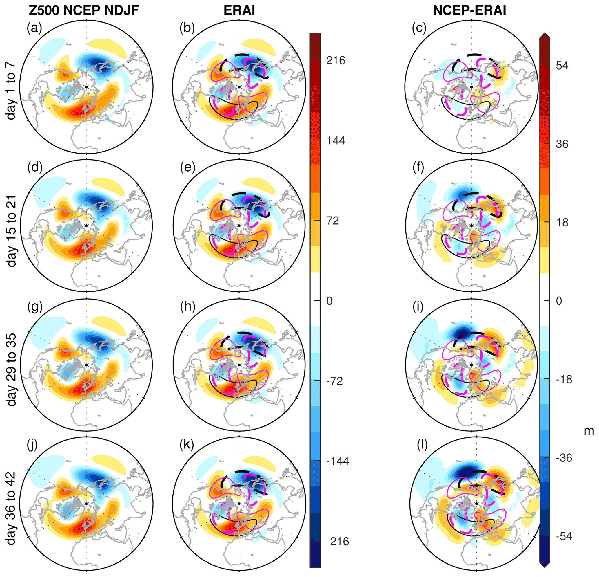
Figure 1Anomalies from zonal mean of geopotential height (m) for initializations during NDJF in the NCEP model during (a) week 1, (d) week 3, (g) week 5, and (j) week 6. The middle column (b, e, h, k) is for ERA-I subsampled to match the dates chosen for NCEP; the right column (c, f, i, l) is for the difference between ERA-I and NCEP; black and magenta contours denote the stationary wavenumber 1 and wavenumber 2 components in ERA-I with contour intervals of ±60 and ±40 m, respectively, with dashed (solid) contours representing negative (positive) anomalies.
During the first week, biases in the stationary wave field are small over the mid-high latitudes. However, during week 3, biases are already developed, with strong positive and negative biases over the northwestern and northeastern Pacific, respectively. In addition, a negative bias develops over the northwestern Atlantic. Following week 3, biases in the North Pacific sector strengthen in magnitude, while those over the North Atlantic slightly strengthen in magnitude and strongly project onto the negative node of wave 2 over the northwestern Atlantic (see magenta contours).
The biases in week 3 for all models (excluding older model versions of ECMWF, UKMO, and Météo-France) are summarized in Fig. 2. The green line corresponds to NCEP, and the other models are shown with other colors. Figure 2a shows a longitudinal cross-section of 500 hPa eddy height field at 50∘ N during week 3 for both the models (solid line) and ERA-I (dashed line), and Fig. 2b shows the biases of the models. In week 3, biases are evident particularly in the ridges over western North America and northern Europe/Atlantic and in the eastward extent of the North Pacific trough. The largest biases are simulated by the ISAC model in western North America and by HMCR, CMA, and BoM over the North Atlantic (Fig. 2b). In the North Pacific sector, the biases are relatively small; however there is a systematic tendency towards a trough that does not extend far enough eastward (NCEP the lone exception).
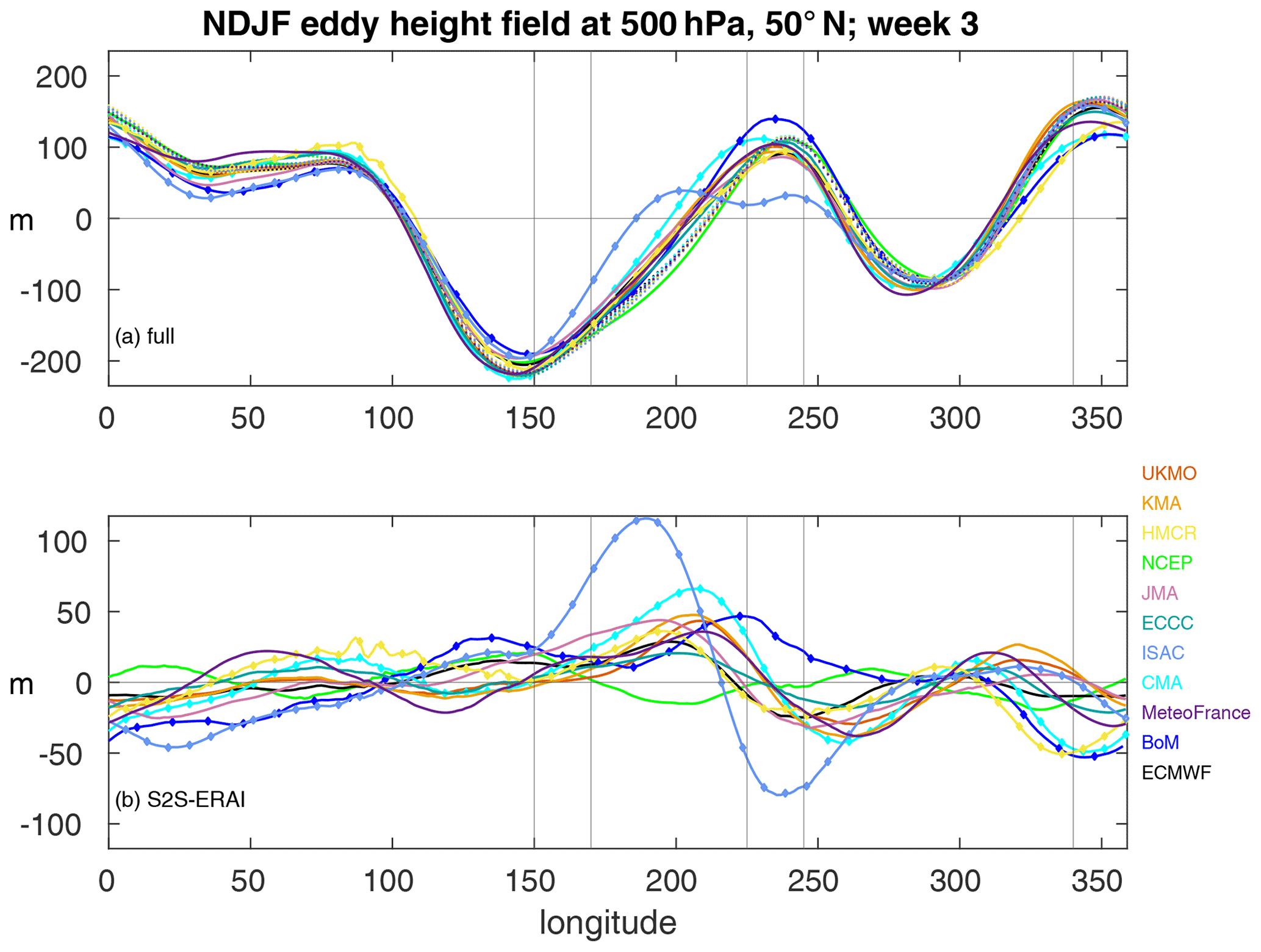
Figure 2Longitudinal cross-section of 500 hPa eddy geopotential height at 50∘ N during NDJF for S2S models (solid lines) and ERA-I (dots) in week 3: (a) S2S models (solid) and ERA-I (dashed), (b) difference between S2S models and corresponding days in ERA-I. Vertical gray lines denote the northwestern Pacific, northwestern North America, and North Atlantic regions used for Fig. 3; low-top models are indicated with diamonds.
As seen in Fig. 2, the mid-tropospheric SWs are strongest in three key regions (North Pacific, western North America, and North Atlantic), and the two ridges in particular are poorly simulated in some models. Figure 3a–c demonstrate the development of weekly lead-time SW biases for initializations during NDJF, with a mid-latitude (40–60∘ N) cross-section of 500 hPa stationary eddy height in these three key regions, respectively, in both the models (solid lines) and the corresponding days in reanalysis (dots).
In the northwestern Pacific (150–170∘ E), about half of the models are already biased 1 week after initialization, and the bias persists throughout the run (Fig. 3a). However, the bias is relatively small. The BoM model, which has the largest bias, reaches a maximal error of approximately 10 % in week 2, while other models have even a smaller bias. Note that the ECMWF 2019 model (thin black line) simulates a too-shallow trough in the NW Pacific at all lead times, while during the first 4 weeks the observed trough deepens, resulting in an increase in the bias. The CMA, JMA, HMCR, BoM, and ISAC models are biased from week 1. In contrast, the UKMO 2019, CNRM 2019, and KMA simulate biases of less than 5 % of the NW Pacific trough throughout the run, while the ECCC model is the only model that almost accurately simulates the trough during all weeks. Other models simulate imperceptible biases for the NW Pacific trough in week 1, but afterwards biases grow.
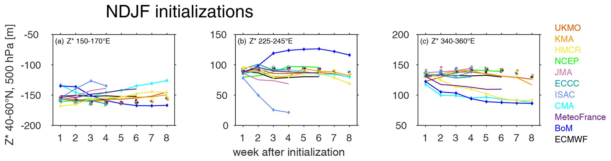
Figure 3Time evolution of simulated 500 hPa stationary eddy height at 40 to 60∘ N in three key regions for all models (solid lines) and corresponding days in ERA-I (dots): (a) northwestern Pacific (150–170∘ E), (b) western North America (225–245∘ E), (c) North Atlantic (340–360∘ E).
While the biases in the northwestern Pacific are less than 10 % of the observed trough for all models, biases are relatively larger in the other regions. In western North America (225–245∘ E), the spread among models is relatively small by the end of week 1, although the bias of the simulated stationary ridge over this region becomes larger at later lags (Fig. 3b). The BoM and ISAC models stand out as very poorly performing during all weeks following week 1. Both either strongly overestimate (BoM) or underestimate (ISAC) the ridge. The JMA and the ECMWF models fail to maintain the magnitude of the observed ridge, and after week 1, its simulated amplitude is ∼10 % weaker than observed. Similar to their realistically simulated trough in the NW Pacific, the ECCC and NCEP models perform well in their simulation of the ridge in western North America, despite a slight positive bias in week 2. All other models diverge from observations in weeks 2–3, with a weaker-than-observed ridge.
Figure 3c indicates that almost all models (NCEP the lone exception) underestimate the strength of the upper-tropospheric North Atlantic stationary ridge (340–360∘ E) during NDJF. In particular, the CNRM, HMCR, BoM and CMA models poorly simulate the ridge at all lags following week 1, and although other models perform better in the North Atlantic region, most of them also simulate a weaker ridge than that observed during all weeks after week 1. These results are consistent with those that have been shown in previous works using CMIP climate models, such as Garfinkel et al. (2020) and Park and Lee (2021), who demonstrate that general circulation models (GCMs) struggle to produce a realistic and strong enough SW in the North Atlantic upper troposphere.
Overall, the models are more biased over western North America and over the North Atlantic compared to the northwestern Pacific region beyond week 2–3 and in some cases, even beyond week 1.
In the previous section, we focus on the mid-tropospheric SWs. Now, we focus on the stratospheric SWs, which are crucial for both realistically simulated mean circulation in the stratosphere (as we soon show) and temporal variability in the polar vortex. Figures 4a–i and 5a–i show the observed and modeled NDJF stationary wave structure in both the troposphere and stratosphere for the NCEP and CMA models, respectively, during week 3 of the integration, when most model simulations start to deviate from observations. In the mid-troposphere, the NCEP model simulates a slightly weaker trough over the northwestern Pacific, but the trough extends too far downstream to the eastern Pacific, as compared to ERA-I (Fig. 4a–c). The amplitude of the biases in NCEP pale in comparison to those in CMA, however. Namely, the CMA model suffers from weaker ridges over western North America and the northern Euro-Atlantic region and a weaker trough in the North Pacific. In the stratosphere, biases are small in the NCEP model, though the biases in the Pacific sector are still present but decay in the mid-stratosphere at 50 hPa (Fig. 4). The projection of the stratospheric biases onto the climatological wave 1 and wave 2 pattern is weak in NCEP. The CMA model, on the other hand, does worse in the stratosphere, with a strong underestimation of the predominant wave 1 in both the lower and mid-stratosphere that projects onto and destructively interferes with climatological wave 1. Additional models are considered in the Supplement. In the ECMWF 2020 model, the strong biases at 500 hPa are mostly evident in western North America, where the ridge is too weak (Fig. S1 in the Supplement), while the BoM, HMCR, and ISAC models are strongly biased over both the North Pacific and the North Atlantic at 500 hPa (Fig. S5, S7, and S9, respectively). In the stratosphere, biases in the CNRM 2019 model mostly project onto the stationary wave 2. In the NCEP, ECMWF 2016, UKMO 2016 and 2020, and the KMA models, biases in the stratosphere project onto stationary wave 2, comparable to the biases in the CNRM model, with the KMA and JMA (in the lower stratosphere) models the least biased (see Supplement). The BoM has a biased wave 2 in the lower stratosphere, while in the mid-stratosphere it is mostly biased towards wave 1 (Fig. S5d–i). In the models that struggle to simulate a realistic wave 2 structure, the simulated wave 1, which is predominant in the stratosphere, is still reasonably simulated; therefore, the simulated mean circulation is not expected to be strongly biased. This stands in contrast to the BoM and CMA models that have strongly biased wave 1 in the stratosphere.

Figure 4Top: anomalies from zonal mean of geopotential height (m) during week 3 for initializations during NDJF in the NCEP model at (a) 500 hPa, (d) 100 hPa, and (g) 50 hPa. The middle column (b, e, h) is for ERA-I subsampled to match the dates chosen for NCEP; the right column (c, f, i) is for the difference between ERA-I and NCEP. Bottom: ω (color) and zonal wind (contours) during week 3 for initializations during NDJF (j) in the NCEP model, (k) for ERA-I to subsampled to match the dates chosen for NCEP, and (i) the difference between ERA-I and NCEP. Black and magenta contours denote the stationary wavenumber 1 and wavenumber 2 components in ERA-I with contour intervals of ±60 and ±40 m, respectively, with dashed (solid) contours representing negative (positive) anomalies. Contour intervals in panels (j) and (k) are at 30 and 60 m s−1 and in panel (l) are at ±2, ±4, ±6, ±8, and ±10 m s−1.
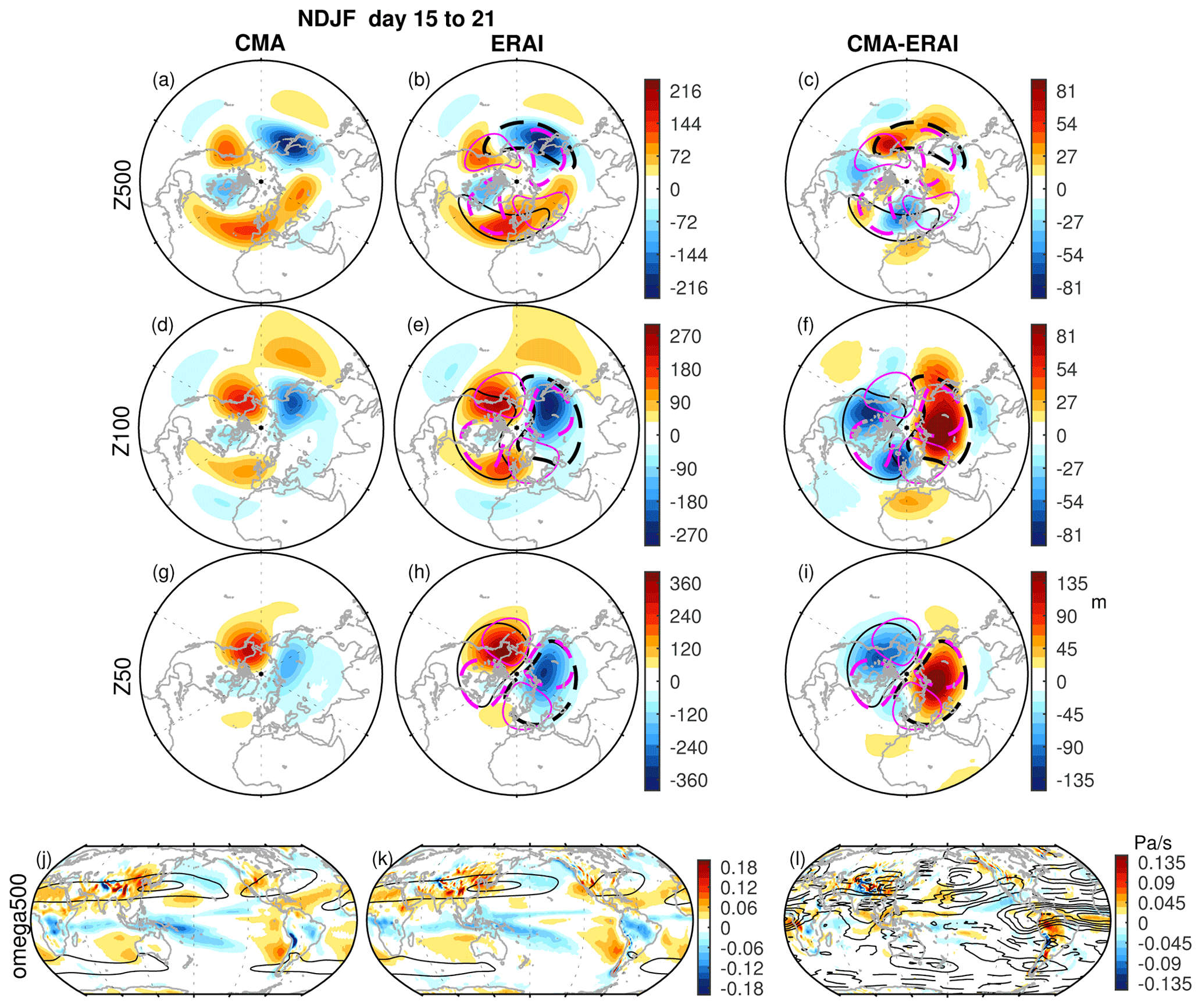
Figure 5Same as Fig. 4 but for the CMA model.
To better demonstrate the effect the regional biases in the troposphere have on the planetary-scale time-mean tropospheric NH circulation, which is particularly relevant for the stratospheric mean state, we compare in Fig. 6 biases in the regional SW field to those in the amplitude of the stationary wave 1 and wave 2, obtained by Fourier decomposition.
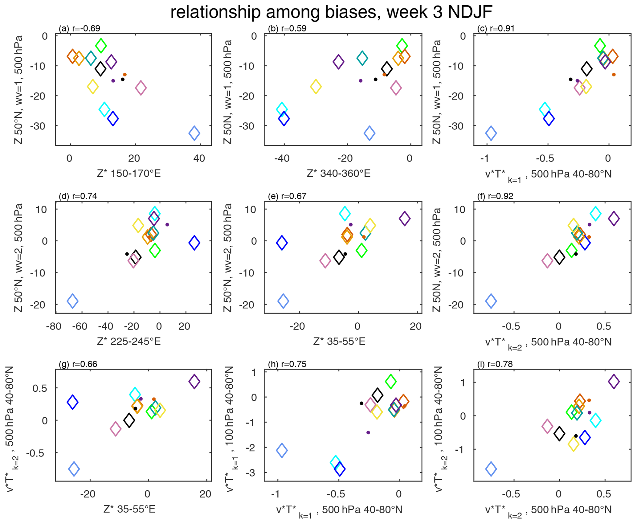
Figure 6Summary of relationships among the biases in the S2S models during NDJF (the different models are represented by colors similarly to the legend of Fig. 3). Panels (a)–(c): Z at 50∘ N wavenumber 1 and (a) 500 hPa Z* over the northwestern Pacific (150–170∘ E), (b) 500 hPa Z* over the North Atlantic (340–360∘ E), and (c) 500 hPa mid-latitude (40–80∘ N) wavenumber 1 . Panels (d)–(f): Z at 50∘ N wavenumber 2 and (d) 500 hPa Z* over western North America (225–245∘ E), (e) 500 hPa Z* over western Eurasia (35–55∘ E), and (f) 500 hPa mid-latitude (40–80∘ N) wavenumber 2 . Panels (g)–(i): (g) 500 hPa mid-latitude (40–80∘ N) wavenumber 2 and 500 hPa Z* over western Eurasia (35–55∘ E), (h) 100 hPa mid-latitude (40–80∘ N) wavenumber 1 and 500 hPa mid-latitude (40–80∘ N) wavenumber 1 , (i) 100 hPa mid-latitude (40–80∘ N) wavenumber 2 and 500 hPa mid-latitude (40–80∘ N) wavenumber 2 ; r denotes the correlation between indices; dots are for older versions of ECMWF, UKMO, and CNRM; all correlations are significant at the 95 % level using a two-tailed Student t test.
Figure 6a contrasts biases in the northwestern Pacific trough with the zonal wavenumber 1 component of the eddy height field at 500 hPa. From Fig. 6a, it is evident that models with a weaker-than-observed northwestern Pacific trough also have too weak of a wave 1 (). The same relationship is evident for wave 2 (; not shown). Over the North Atlantic, a shallower ridge is associated with a biased too-weak wave 1 with a correlation of r=0.59 (Fig. 6b). Figure 6c contrasts the magnitude of the wave 1 component of eddy height with wave 1 heat flux at 500 hPa and indicates a strong connection (r=0.91), as expected from Garfinkel et al. (2010). Figure 6d and e also show a strong connection between mid-tropospheric wave 2 biases and regional biases over western North America (r=0.74) and over western Eurasia (r=0.67), respectively. Similarly to wave 1, a strong relationship is evident between biases in wave 2 mid-tropospheric height and biases in the wave 2 component of meridional eddy heat flux (Fig. 6f). The importance of the western Eurasian ridge to upward coupling of wave 2 has been stressed in previous works such as Garfinkel et al. (2019) and Karpechko et al. (2018). In both works, an error in the simulated western Eurasian ridge in S2S models is linked to a weaker simulated upward propagation of planetary wave activity and, as a result, erroneous stratospheric variability. Figure 6g demonstrates that this connection is present in the time mean, with biases over western Eurasia significantly linked to biases in upward propagation of planetary wave 2 activity, indicated by biases in mid-tropospheric wave 2 meridional eddy heat flux (r=0.66).
The connection of biases in the mid-troposphere to biases in lower-stratospheric planetary wave activity is shown in Fig. 6h and i for wave 1 and wave 2, respectively. In both cases, models that are more biased in their simulated wave 1 and wave 2 in the mid-troposphere are also more biased in their upward coupling of wave 1 (r=0.75) and wave 2 (r=0.78).
In general, the connection between the regional biases and the planetary wave 1 and wave 2 is strong across all regions. In particular, biases in regional mid-tropospheric SWs are closely related to biases in wave 1 and wave 2 meridional eddy heat flux, which in turn lead to a biased wave activity that enters the stratosphere.
The wintertime stratospheric polar vortex in the NH is weaker than its Southern Hemisphere (SH) counterpart. This is because of the time-mean stationary waves and in particular the wavenumber 1 and 2 components that originate in the troposphere. Therefore, a key ingredient for a realistic stratospheric mean state is realistic time-mean eddy fluxes originating in the troposphere. Figure 7 shows the time evolution of meridional heat flux of wavenumbers 1 and 2 and the stratospheric polar vortex (zonal mean at 60∘ N), for both the models (solid lines) and the corresponding days in reanalysis (dots) during NDJF. We examine both the mid-tropospheric and lower-stratospheric meridional eddy heat flux over the mid-latitudes (40–80∘ N), , which is used as a proxy for upward coupling between the troposphere and the stratosphere.
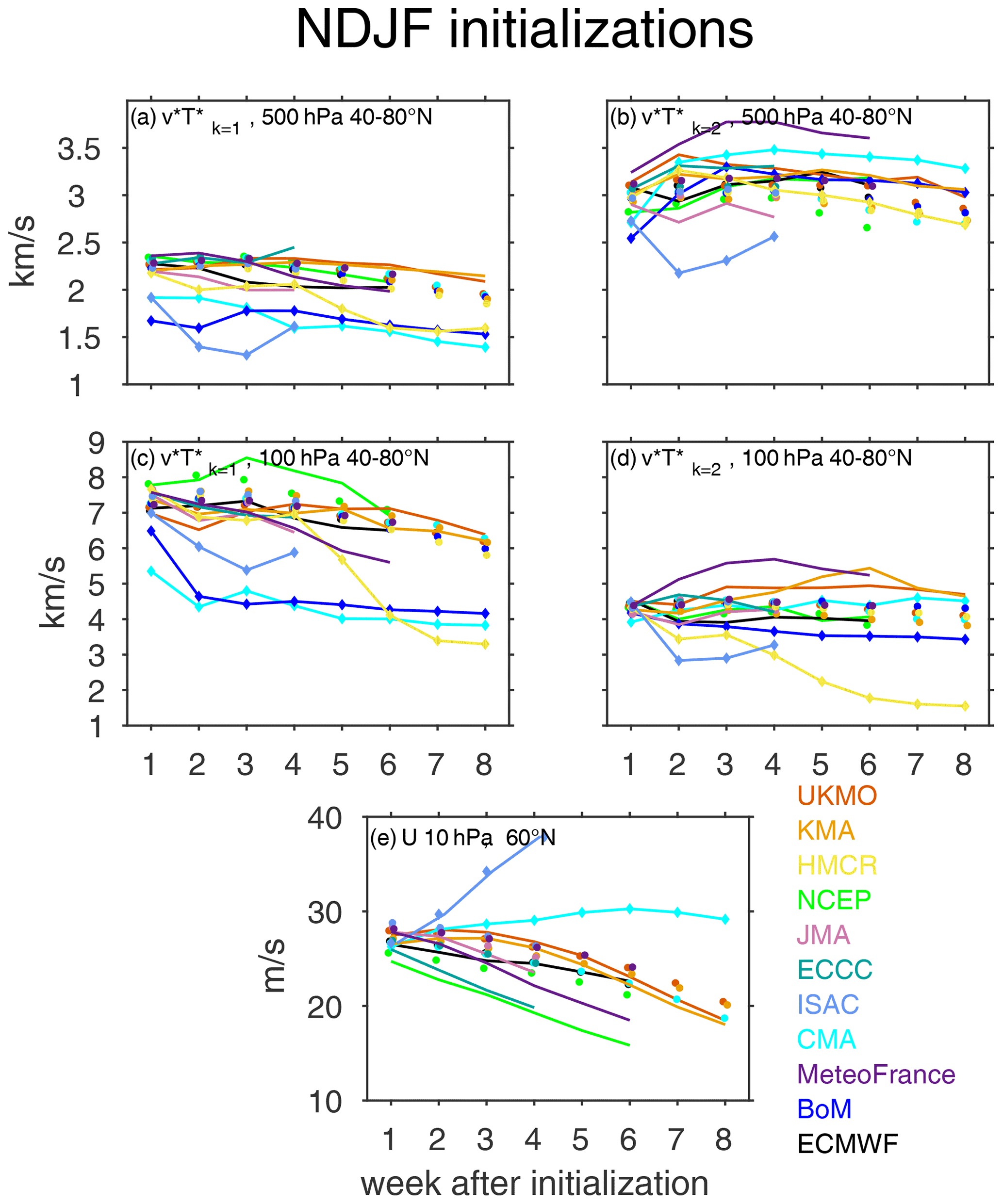
Figure 7Time evolution of all integrations during November–December–January–February for S2S models (solid lines) and corresponding days from ERA-I (dots). (a) Mid-latitude wave 1 at 500 hPa, (b) mid-latitude wave 2 at 500 hPa, (c) mid-latitude wave 1 at 100 hPa, (d) mid-latitude wave 2 at 100 hPa, (e) zonal-mean zonal wind at 10 hPa at 60∘ N. Low-top models are indicated with diamonds on the line.
In the mid-troposphere, wave 1 is better simulated by NCEP, UKMO, ECCC, and the KMA models. The ECMWF, JMA, and to a lesser degree CNRM at later weeks underestimate the amplitude, particularly following week 2. The biases are much more pronounced in the low-top models than in any of the aforementioned high-top models. Specifically, the amplitude in the BoM, ISAC, HMCR (to a lesser degree), and CMA is poorly simulated, and the bias is large already in week 2 (Fig. 7a). For mid-tropospheric wave 2, too-strong biases exist in the NCEP, ECMWF, and UKMO models after week 3, while the models that fail to simulate realistic amplitudes are the CMA, CNRM 2019, and ISAC (Fig. 7b). Only the HMCR model shows consistency, with small biases throughout the run.
In the lower stratosphere, biases in are noticeable in most models. For wave 1, the KMA and ECMWF models decently simulate wave 1 throughout the run, while the UKMO model has a slightly weaker wave 1 signal than that observed during weeks 2–4, but then it simulates the amplitudes very well. Nevertheless, other models struggle to simulate a realistic wave 1 throughout the run. The NCEP model largely overestimates the amplitude of wave 1 following week 2, while the CMA, ISAC, and BoM models considerably underestimate its amplitude after week 1 (Fig. 7c). Similarly to the mid-troposphere, the CNRM and JMA models start with a relatively realistic wave 1 amplitude during the first 2 weeks, but then the simulated amplitude weakens compared to observations. For wave 2 shown in Fig. 7d, the UKMO and KMA models overestimate the amplitude following week 3, whereas the ECMWF slightly underestimates the amplitude from week 2. The CNRM 2019 model has the largest positive bias of any model, while BoM, ISAC, and HMCR all have a substantially too-weak wave 2 bias after week 1, though their negative bias is not as large as in wave 1. The CMA has a decently simulated amplitude of wave 2 during the first 6 weeks of the integration, despite its poorly simulated wave 2 amplitude in the mid-troposphere. In contrast to its overly strong wave 1, the simulated wave 2 in the NCEP model is relatively realistic.
As mentioned earlier, during winter, the presence of stationary wavenumbers 1 and 2 in the stratosphere is the reason for a weakened vortex relative to its SH winter counterpart, which enables transients to propagate into the stratosphere and perturb the vortex even further. Therefore, a realistically simulated mean-state vortex is an important factor for upward wave propagation and vortex daily variability. Figure 7e shows the time evolution of the stratospheric polar vortex, represented as the 10 hPa zonal-mean zonal wind at 60∘ N in both models and reanalysis. Consistent with the large negative bias of wave 1 in the lower stratosphere, the CMA and ISAC models simulate a too-strong polar vortex. The NCEP model starts with a realistic vortex strength during the first week, but then diverges from observations and simulates a weaker vortex that becomes even weaker as the run progresses. This is congruent with the substantial positive bias of wave 1 in the lower stratosphere shown in Fig. 7c. The KMA, ECMWF, and UKMO models show only small biases, which may be a result a successful simulation of wave 1 in the lower stratosphere by these models. Similar to the NCEP model, the CNRM 2019 model also simulates a too-weak polar vortex following the first week, but in contrast, this is possibly more due to the positive bias in wave 2 shown in Fig. 7d. Interestingly, the ECCC is unable to simulate a realistic polar vortex after the first week, despite its decently simulated waves 1–2 in both the mid-troposphere and lower stratosphere.
Overall, the CMA, HMCR, ISAC, and BoM models, i.e, those with a low-resolution stratosphere (the latter three are also low-top), struggle to simulate realistic , particularly in the stratosphere, which may be a result of poorly represented upward coupling. This, in turn, affects the stratospheric mean-state zonal circulation, and as a consequence, temporal variability is too weak, as demonstrated in previous works (Domeisen et al., 2020a; Schwartz and Garfinkel, 2020). Despite its high model top and stratospheric resolution, the NCEP and CNRM 2019 models have a too-weak vortex strength during winter, which is a result of too strong a wave flux in the lower stratosphere for wave 1 and wave 2, respectively.
As noted in Sect. 1, the biases in the stationary wave pattern, in both the troposphere and the stratosphere, may be a result of a poorly represented time-mean tropical convection. For example, deep convection in the tropical western Pacific may be one of the drivers that directly (Hoskins and Karoly, 1981; Jin and Hoskins, 1995) and indirectly (Simmons et al., 1983) form a Pacific–North American (PNA)-like pattern. Figures 4 and 5 show the time-mean pressure velocity, ω, and zonal winds during week 3 of the integration in the NCEP and CMA models (panel j), the corresponding days in ERA-I (panel k), and the bias (panel l). In the NCEP model, tropical convection is weaker over the Maritime Continent region compared to ERA-I. This might contribute to the too-weak low and a too-strong downstream extension of the low to the central and eastern Pacific that was evident in Fig. 4. Consistent with this, the northward-directed flux of Takaya and Nakamura (2001) is too weak in the western Pacific and too strong in the eastern Pacific (not shown). In the CMA model, the tropical convection along the South Pacific Convergence Zone (SPCZ) is slightly stronger than that observed, but even more evident are the biases in the mean zonal flow that extend from the eastern Pacific far into the North Atlantic and may contribute to errors in Rossby wave generation and propagation. The positive bias in ω over the Maritime Continent and West Pacific Warm Pool is evident in all other models (see Supplement).
Next, we examine the regional biases in the tropics that possibly have an impact on the extratropical mean state. Figure 8 shows a longitudinal cross-section of 500 hPa ω, averaged between 15∘ S–10∘ N, during week 3 of integration in the models (solid line) and the corresponding days in ERA-I (dots) in panel a, while the bias of the models is in panel b.

Figure 8Longitudinal cross-section of NDJF 500 hPa pressure–velocity (ω) averaged between 15∘ S–10∘ N during week 3 of integration for (a) S2S models (solid lines) and corresponding days in ERA-I (dots) and (b) the difference between S2S models and the corresponding days in ERA-I.
From panel a, there are three main convection centers along the tropics during NDJF: over Central Africa, the Maritime Continent/western Pacific, and the Amazon. Previous works have shown that convection in these regions can impact the extratropical North Pacific and North Atlantic circulation (Hoskins and Ambrizzi, 1993; Jin and Hoskins, 1995). Panel b shows that biases in the models, in large, are confined to these regions and extend to the eastern Pacific as well. The performance of the models in simulating realistic mean tropical convection is not the goal of this paper; however, the divergent wind and subtropical convergence and downwelling in the Northern Hemisphere associated with this tropical upwelling can help seed Rossby waves (Sardeshmukh and Hoskins, 1988). Therefore, we focus now on how the biases in three regions within the tropics and subtropics are connected to the simulation of SWs in the key regions in the extratropics.
Figure 9 summarizes the relationships between NDJF 500 hPa ω biases in the subtropical western Pacific, tropical eastern Pacific, and the Caribbean and the extratropical mid-tropospheric stationary height biases in the North Pacific, western North America, and the North Atlantic, respectively, during week 3 of integration. Note that following Sardeshmukh and Hoskins (1988), Rossby wave sources (RWSs) are formed in regions of downwelling (and upper-tropospheric convergence). Therefore, we examine subtropical regions where downwelling is considerably strong as a result of tropical convection in the deep tropics. One exception is the deep tropical eastern Pacific, which is located in the descending branch of the Walker Cell and is embedded in the mean upper-tropospheric westerlies and therefore is able to seed poleward-propagating Rossby waves despite being closer to the Equator.
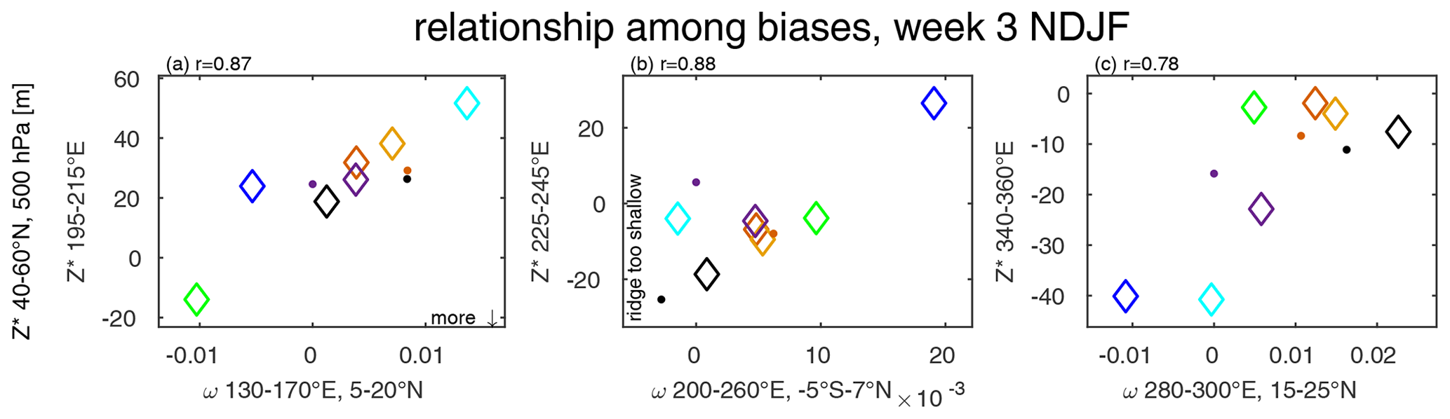
Figure 9Summary of relationship among mid-latitude (40–60∘ N) regional biases of 500 hPa Z* over (a) the northwestern Pacific (195–215∘ E) and ω over the subtropical western Pacific (5–20∘ N, 130–170∘ E), (b) western North America (225–245∘ E) and 500 hPa ω over the tropical eastern Pacific (5∘ S–7∘ N, 200–260∘ E), and (c) the North Atlantic (340–360∘ E) and ω over the Caribbean (15–25∘ N, 280–300∘ E); r denotes the correlation between indices; dots are for older versions of ECMWF, UKMO, and CNRM; and all correlations are significant at the 95 % level. Note that for panel (a), we focus on the eastward extension of the North Pacific low, which differs more dramatically among the models, rather than the northwestern Pacific low itself, which is better represented by the models.
Figure 9a indicates that a weaker eastward extension of the trough over the mid-troposphere North Pacific is associated with a too-strong downwelling compared to that observed in the subtropical western Pacific (r=0.87). Over the eastern Pacific, enhanced descending motion is positively correlated with a stronger ridge over western North America (Fig. 9b; r=0.88). Similarly, downwelling near the Caribbean is associated with a North Atlantic ridge (r=0.78). In general, Fig. 9 shows that biases over lower latitudes have a direct impact on the simulated SWs in the extratropics. These biases in convection are already present in week 1 (Fig. S13) and hence develop before the biases in the mid-latitude stationary waves, indicating that the tropical biases lead to extratropical biases rather than the reverse.
Figure 9 demonstrated a connection between ω in specific regions and the extratropical SWs; however it is important to note that robust correlations are also evident in other regions, and hence the relationships in Fig. 9 do not unambiguously demonstrate a connection. Specifically, Fig. S14 shows the correlation between regional 500 hPa Z* height biases and ω for each of the three regions of Fig. 9. In addition to the regions enclosed with boxes which we focus on for Fig. 9, correlations are evident elsewhere. Hence future work is needed to demonstrate a causal connection; however it is well known that tropical and subtropical divergence and convergence can help seed Rossby waves propagating poleward. In summary, biases emanating from erroneous simulation of tropical convection in the models are associated with the strength of the extratropical NH stationary SWs and result in a biased response over the Pacific and Atlantic mid-upper troposphere.
The Northern Hemisphere SWs play a major role in fluxing heat and momentum away from the subtropics as well as modulating the storm tracks and large-scale circulation in both the troposphere and stratosphere. In particular, realistically simulated SWs by global atmospheric models used for both future climate projections and medium-range forecasts are crucial for accurate weather and climate surface predictions, which have significant and potentially life-saving societal and economic implications.
In this work, we investigated how well tropospheric and stratospheric planetary SWs are simulated in 11 operational subseasonal models during NDJF. We showed that biases in the troposphere evolve with lead time and are pronounced already by week 2–3. Nearly all models have like-signed biases over the North Pacific, western North America, and North Atlantic regions, regions where the amplitude of SWs peaks, and nearly all models simulate too weak a SW in these regions. More specifically, it has been shown that the biases in the North Pacific sector are already evident from week 1, in both amplitude and phase. However, they are smaller compared to those over the western North America and North Atlantic regions; specifically some models suffer from biases of 50 % or more in the northwestern North American and North Atlantic ridge.
We also considered SW biases in the context of troposphere–stratosphere upward coupling, with a particular emphasis on wave 1 and wave 2, which are particularly relevant to upward propagation of waves into the stratosphere. In the troposphere, the models vary in their ability to simulate wave 1 meridional eddy heat flux, while wave 2 is at least decently simulated by most of them, with the KMA model the most realistic in simulated wave 1 and wave 2. Next, we showed that a connection exists between regional biases of SWs in the troposphere and upward propagation of planetary waves, further stressing the importance of realistically simulated SWs in key regions in the mid-latitude troposphere.
In the stratosphere, it is demonstrated that the models with finer vertical resolution in the stratosphere and high model top generally do a better job in simulating the stratospheric mean state and potentially are more skillful in forecasting variability in the stratosphere on subseasonal timescales (Domeisen et al., 2020b). Interestingly, models with a less complex stratosphere have a more biased wave 1, while those with a finer vertical resolution generally represent wave 1 well but tend to have biases in their simulated wave 2. It is not clear if this difference might be a result of small sample size or alternately a systematic effect of stratosphere complexity in the models. Nevertheless, a more complex stratosphere is only one ingredient for a realistic stratospheric mean state as demonstrated in the case of the NCEP model, which is positively biased in its wave 1 meridional heat flux in the lower stratosphere, and as a result, its simulated time-mean polar vortex is too weak, even as its tropospheric SWs and heat flux are well represented. This is also shown in Butler et al. (2016), who showed that the models that participated in the Climate System Historical Forecast Project with a higher-complexity stratosphere are not necessarily better skilled in forecasting seasonal sea-level pressure over the North Pole regions in winters when no SST anomalies are present in the tropical Pacific. Nevertheless, biases in the stratospheric SWs are closely related to biases in the tropospheric SWs, and overall high-top models do a better job in both the troposphere and stratosphere. In addition, radiative processes can also contribute to mean-state biases in the stratosphere, and future work should consider the relative role of radiative vs. dynamical processes for mean-state biases.
Finally, we also considered whether biases in the tropics and subtropics may play a role in the simulated tropospheric mid-latitude SW field in the models. Large biases in the models are evident in oceanic basins immediately to the south and west of the strongest features of the SW pattern, namely in the western Pacific, eastern Pacific, and Caribbean. We examined whether regional biases in SWs are related to a biased subtropical (and tropical in the case of the eastern Pacific) downwelling and found a significant connection in the models between a biased downwelling in the subtropical western Pacific and Caribbean and biases in the northwestern Pacific trough and northwestern Atlantic. In addition, a significant relationship exists between downwelling in the tropical eastern Pacific, associated with the descending branch of the Walker Cell, and the western North America ridge. This apparent relationship between subtropical and tropical downwelling and mid-latitude SWs does not demonstrate causality however, and further work that integrates both the models’ mean state and idealized modeling has to be done in order to better identify sources for SW biases in the S2S models.
Our results demonstrate the importance of accurately simulated SWs for both the tropospheric and stratospheric mean state in the models. Most subseasonal models, and in particular low-top models, show little consistency in their simulated SWs at lead times longer than 1–2 weeks, which may enhance forecast errors on subseasonal timescales, particularly those induced by the stratospheric variability. This has significant implications on forecast skill of timescales longer than 1–2 weeks, as demonstrated in Domeisen et al. (2020b), who showed that high-top S2S models have higher predictability skill of stratospheric variability compared to low-top models and therefore better simulate the surface impacts on subseasonal timescales.
Overall, it is shown that a well-simulated SW field in the troposphere is a necessary, though not sufficient ingredient for a realistically simulated stratospheric mean circulation, which in turn enables more accurate temporal variability and surface predictability on subseasonal timescales.
This work is based on S2S data. S2S is a joint initiative of the World Weather Research Programme (WWRP) and the World Climate Research Programme (WCRP). The original S2S database is hosted at the ECMWF as an extension of the TIGGE database and can be downloaded from the ECMWF server: http://apps.ecmwf.int/datasets/data/s2s/levtype=sfc/type=cf/ (Vitart et al., 2017).
The supplement related to this article is available online at: https://doi.org/10.5194/wcd-3-679-2022-supplement.
CIG initiated and designed the study; CS provided the data and the majority of writing; and PY, WC, and DIVD gave comments and contributed to the writing and analysis.
The contact author has declared that neither they nor their co-authors have any competing interests.
Publisher’s note: Copernicus Publications remains neutral with regard to jurisdictional claims in published maps and institutional affiliations.
We sincerely thank Ian P. White for the meaningful discussion throughout the work.
Chaim I. Garfinkel, Chen Schwartz, and Wen Chen are supported by the ISF‐-NSFC joint research program (grant no. 3259/19), and Daniela Domeisen and Priyanka Yadav are supported by the Swiss National Science Foundation through projects PP00P2_170523 and PP00P2_198896.
This paper was edited by Silvio Davolio and reviewed by two anonymous referees.
Baldwin, M. P., Ayarzagüena, B., Birner, T., Butchart, N., Butler, A. H., Charlton-Perez, A. J., Domeisen, D. I., Garfinkel, C. I., Garny, H., Gerber, E. P., Heggelin, M. I., Langematz, U., and Pedatella, N. M.: Sudden stratospheric warmings, Rev. Geophys., 59, e2020RG000708, https://doi.org/10.1029/2020RG000708, 2021. a
Butler, A. H., Arribas, A., Athanassiadou, M., Baehr, J., Calvo, N., Charlton-Perez, A., Déqué, M., Domeisen, D. I., Fröhlich, K., Hendon, H., Imada, Y., Ishii, M., Iza, M., Karpechko, A. Y., Kumar, A., MacLachlan, C., Merryfield, W. J., Müller, W. A., O'Neill, A., Scaife, A. A., Scinocca, J., Sigmond, M., Stockdale, T. N., and Yasuda, T.: The Climate-system Historical Forecast Project: do stratosphere-resolving models make better seasonal climate predictions in boreal winter?, Q. J. Roy. Meteor. Soc., 142, 1413–1427, 2016. a
Charney, J. G. and Drazin, P. G.: Propagation of planetary-scale disturbances from the lower into the upper atmosphere, J. Geophys. Res., 66, 83–109, https://doi.org/10.1029/JZ066i001p00083, 1961. a
Cohen, J. and Jones, J.: Tropospheric Precursors and Stratospheric Warmings, J. Climate, 24, 6562–6572, https://doi.org/10.1175/2011JCLI4160.1, 2011. a
Dee, D. P., Uppala, S. M., Simmons, A. J., Berrisford, P., Poli, P., Kobayashi, S., Andrae, U., Balmaseda, M., Balsamo, G., Bauer, d. P., Bechtold, P., Beljaars, A. C. M., van de Berg, L., Bidlot, J., Bormann, N., Delsol, C., Dragani, R., Fuentes, M., Geer, A. J., Haimberger, L., Healy, S. B., Hersbach, H., Hólm, E. V., Isaksen, L., Kållberg, P., Köhler, M. Matricardi, M., McNally, A. P., Monge-Sanz, B. M., Morcrette, J.-J., Park, B.-K., Peubey, C., de Rosnay, P., Tavolato, C., Thépaut, J.-N., and Vitart, F.: The ERA-Interim reanalysis: Configuration and performance of the data assimilation system, Q. J. Roy. Meteor Soc., 137, 553–597, 2011. a
Domeisen, D. I. and Plumb, R. A.: Traveling planetary-scale Rossby waves in the winter stratosphere: The role of tropospheric baroclinic instability, Geophys. Res. Lett., 39, 0094–8276, 2012. a
Domeisen, D. I., Martius, O., and Jiménez-Esteve, B.: Rossby wave propagation into the Northern Hemisphere stratosphere: The role of zonal phase speed, Geophys. Res. Lett., 45, 2064–2071, 2018. a
Domeisen, D. I. V., Butler, A. H., Charlton-Perez, A. J., Ayarzagüena, B., Baldwin, M. P., Dunn-Sigouin, E., Furtado, J. C., Garfinkel, C. I., Hitchcock, P., Karpechko, A. Y., Kim, H., Knight, J., Lang, A. L., Lim, E.-P., Marshall, A., Roff, G., Schwartz, C., Simpson, I. R., Son, S.-W., and Taguchi, M.: The Role of the Stratosphere in Subseasonal to Seasonal Prediction: 2. Predictability Arising From Stratosphere-Troposphere Coupling, J. Geophys. Res.-Atmos., 125, 2169–897X, https://doi.org/10.1029/2019jd030923, 2020a. a, b
Domeisen, D. I. V., Butler, A. H., Charlton-Perez, A. J., Ayarzagüena, B., Baldwin, M. P., Dunn-Sigouin, E., Furtado, J. C., Garfinkel, C. I., Hitchcock, P., Karpechko, A. Y., Kim, H., Knight, J., Lang, A. L., Lim, E.-P., Marshall, A., Roff, G., Schwartz, C., Simpson, I. R., Son, S.-W., and Taguchi, M.: The Role of the Stratosphere in Subseasonal to Seasonal Prediction: 1. Predictability of the Stratosphere, J. Geophys. Res.-Atmos., 125, 2169–897X, https://doi.org/10.1029/2019jd030920, 2020b. a, b, c
Garfinkel, C. I. and Hartmann, D. L.: Different ENSO Teleconnections and Their Effects on the Stratospheric Polar Vortex, J. Geophys. Res.-Atmos., 113, 0148–0227, https://doi.org/10.1029/2008JD009920, 2008. a
Garfinkel, C. I., Hartmann, D. L., and Sassi, F.: Tropospheric Precursors of Anomalous Northern Hemisphere Stratospheric Polar Vortices, J. Climate, 23, 3282–3299, https://doi.org/10.1175/2010jcli3010.1, 2010. a, b
Garfinkel, C. I., Schwartz, C., Domeisen, D. I. V., Son, S.-W., Butler, A. H., and White, I. P.: Extratropical Atmospheric Predictability From the Quasi-Biennial Oscillation in Subseasonal Forecast Models, J. Geophys. Res.-Atmos., 123, 7855–7866, https://doi.org/10.1029/2018jd028724, 2018. a
Garfinkel, C. I., Schwartz, C., Butler, A. H., Domeisen, D. I., Son, S.-W., and White, I. P.: Weakening of the teleconnection from El Niño–Southern Oscillation to the Arctic stratosphere over the past few decades: What can be learned from subseasonal forecast models?, J. Geophys. Res.-Atmos., 124, 7683–7696, 2019. a, b
Garfinkel, C. I., White, I., Gerber, E. P., Jucker, M., and Erez, M.: The building blocks of Northern Hemisphere wintertime stationary waves, J. Climate, 33, 5611–5633, 2020. a, b, c, d
Held, I. M., Ting, M., and Wang, H.: Northern winter stationary waves: Theory and modeling, J. Climate, 15, 2125–2144, https://doi.org/10.1175/1520-0442(2002)015<2125:NWSWTA>2.0.CO;2, 2002. a, b
Hoskins, B. J. and Ambrizzi, T.: Rossby Wave Propagation on a Realistic Longitudinally Varying Flow, J. Atmos. Sci., 50, 1661–1671, https://doi.org/10.1175/1520-0469(1993)050<1661:RWPOAR>2.0.CO;2, 1993. a
Hoskins, B. J. and Karoly, D.: The Steady Linear Response of a Spherical Atmosphere to Thermal and Orographic Forcing, J. Atmos. Sci., 38, 1179–1196, 1981. a, b
Jin, F. and Hoskins, B. J.: The direct response to tropical heating in a baroclinic atmosphere, J. Atmos. Sci., 52, 307–319, 1995. a, b
Karpechko, A. Y., Charlton-Perez, A., Balmaseda, M., Tyrrell, N., and Vitart, F.: Predicting Sudden Stratospheric Warming 2018 and Its Climate Impacts With a Multimodel Ensemble, Geophys. Res. Lett., 45, 13–538, 2018. a
Kidston, J., Scaife, A. A., Hardiman, S. C., Mitchell, D. M., Butchart, N., Baldwin, M. P., and Gray, L. J.: Stratospheric influence on tropospheric jet streams, storm tracks and surface weather, Nat. Geosci., 8, 433–440, https://doi.org/10.1038/ngeo2424, 2015. a
Kolstad, E. W., Breiteig, T., and Scaife, A. A.: The association between stratospheric weak polar vortex events and cold air outbreaks in the Northern Hemisphere, Q. J. Roy. Meteor. Soc., 136, 886–893, 2010. a
Limpasuvan, V., Hartmann, D. L., Thompson, D. W. J., Jeev, K., and Yung, Y. L.: Stratosphere-troposphere evolution during polar vortex intensification, J. Geophys. Res., 110, D24101, https://doi.org/10.1029/2005jd006302, 2005. a
Neelin, J. D., Langenbrunner, B., Meyerson, J. E., Hall, A., and Berg, N.: California winter precipitation change under global warming in the Coupled Model Intercomparison Project phase 5 ensemble, J. Climate, 26, 6238–6256, 2013. a
Park, M. and Lee, S.: Is the Stationary Wave Bias in CMIP5 Simulations Driven by Latent Heating Biases?, Geophys. Res. Lett., 48, e2020GL091678, https://doi.org/10.1029/2020GL091678, 2021. a, b
Sardeshmukh, P. D. and Hoskins, B. J.: The Generation of Global Rotational Flow by Steady Idealized Tropical Divergence, J. Atmos. Sci., 45, 1228–1251, 1988. a, b, c
Schwartz, C. and Garfinkel, C. I.: Troposphere-stratosphere coupling in subseasonal-to-seasonal models and its importance for a realistic extratropical response to the Madden-Julian Oscillation, J. Geophys. Res.-Atmos., 125, e2019JD032043, https://doi.org/10.1029/2019JD032043, 2020. a, b, c
Simmons, A., Wallace, J., and Branstator, G.: Barotropic wave propagation and instability, and atmospheric teleconnection patterns, J. Atmos. Sci., 40, 1363–1392, 1983. a
Simpson, I. R., Seager, R., Ting, M., and Shaw, T. A.: Causes of change in Northern Hemisphere winter meridional winds and regional hydroclimate, Nat. Clim. Change, 6, 65–70, 2016. a
Smith, K. L. and Kushner, P. J.: Linear interference and the initiation of extratropical stratosphere-troposphere interactions, J. Geophys. Res.-Atmos., 117, 0148–0227, https://doi.org/10.1029/2012jd017587, 2012. a
Takaya, K. and Nakamura, H.: A formulation of a phase-independent wave-activity flux for stationary and migratory quasigeostrophic eddies on a zonally varying basic flow, J. Atmos. Sci., 58, 608–627, 2001. a
Vitart, F., Ardilouze, C., Bonet, A., Brookshaw, A., Chen, M., Codorean, C., Déqué, M., Ferranti, L., Fucile, E., Fuentes, M., Hendon, H., Hodgson, J., Kang, H.-S., Kumar, A., Lin, H., Liu, G., Liu, X., Malguzzi, P., Mallas, I., Manoussakis, M., Mastrangelo, D., MacLachlan, C., McLean, P., Minami, A., Mladek, R., Nakazawa, T., Najm, S., Nie, Y., Rixen, M., Robertson, A.W., Ruti, P., Sun, C., Takaya, Y., Tolstykh, M., Venuti, F., Waliser, D., Woolnough, S., Wu, T., Won, D.-J., Xiao, H., Zaripov, R., and Zhang, L.: The Subseasonal to Seasonal (S2S) Prediction Project Database, B. Am. Meteorol. Soc., 98, 163–173, https://doi.org/10.1175/BAMS-D-16-0017.1, 2017 (data available at: http://apps.ecmwf.int/datasets/data/s2s/levtype=sfc/type=cf/., last access: 25 May 2021). a, b, c
Watt-Meyer, O. and Kushner, P. J.: The Role of Standing Waves in Driving Persistent Anomalies of Upward Wave Activity Flux, J. Climate, 28, 9941–9954, https://doi.org/10.1175/jcli-d-15-0317.1, 2015. a
- Abstract
- Introduction
- Data and methods
- Fidelity of tropospheric stationary waves in subseasonal models
- Impact of simulated SWs on troposphere–stratosphere upward coupling
- Possible sources for the biases
- Conclusions
- Data availability
- Author contributions
- Competing interests
- Disclaimer
- Acknowledgements
- Financial support
- Review statement
- References
- Supplement