Pacific Decadal Oscillation modulates the Arctic sea-ice loss influence on the midlatitude atmospheric circulation in winter

The modulation of the winter impacts of Arctic sea-ice loss by the Pacific Decadal Oscillation (PDO) is investigated in the IPSL-CM6A-LR ocean–atmosphere general circulation model. Ensembles of simulations are performed with constrained sea-ice concentration following the Polar Amplification Model Intercomparison Project (PAMIP) and initial conditions sampling warm and cold phases of the PDO. Using a general linear model, we estimate the simulated winter impact of sea-ice loss, PDO and their combined effects. On the one hand, a negative North Atlantic Oscillation (NAO)-like pattern appears in response to sea-ice loss together with a modest deepening of the Aleutian Low. On the other hand, a warm PDO phase induces a large positive Pacific–North America pattern, as well as a small negative Arctic Oscillation pattern. Both sea-ice loss and warm PDO responses are associated with a weakening of the poleward flank of the eddy-driven jet, an intensification of the subtropical jet and a weakening of the stratospheric polar vortex. These effects are partly additive; the warm PDO phase therefore enhances the response to sea-ice loss, while the cold PDO phase reduces it. However, the effects of PDO and sea-ice loss are also partly non-additive, with the interaction between both signals being slightly destructive. This results in small damping of the PDO teleconnections under sea-ice loss conditions, especially in the stratosphere. The sea-ice loss responses are compared to those obtained with the same model in atmosphere-only simulations, where sea-ice loss does not significantly alter the stratospheric polar vortex.

1 Introduction

Since the late 1970s, the Arctic sea-ice extent has exhibited a significant decline in all seasons, which is due to human influence (IPCC, 2021) and is expected to continue. Climate models project a summer ice-free Arctic Ocean by 2050, although this date varies depending on the climate scenario considered (SIMIP Community, 2020). Many studies have shown that the Arctic sea-ice loss could change the midlatitude climate, but its extent is still a matter of debate (Cohen et al., 2014; Blackport and Screen, 2020; Hay et al., 2022).

Studies with observations have linked the loss of Arctic sea ice in late autumn to a negative North Atlantic Oscillation (NAO) in winter (King et al., 2016; Garcia-Serrano et al., 2015; Simon et al., 2020). Different physical mechanisms have been proposed to explain the reduced sea ice and negative NAO relationship. It involves a tropospheric pathway, with a reduction of the equatorward-to-pole lower-tropospheric temperature gradient weakening the eddy activity, followed by feedback related to the eddy–mean flow interactions (Smith et al., 2022). A stratospheric pathway was also found, where upward-propagating planetary waves into the stratosphere are intensified with sea-ice loss. Such waves lead to a weakening of the polar vortex propagating downward into an Arctic Oscillation (AO) pattern. However, the observational period is too short to accurately assess the amplitude of sea-ice loss impact. On the one hand, most atmospheric models forced by a reduction of Arctic sea-ice cover simulate a negative NAO-type response in winter (Sun et al., 2015; Peings and Magnusdottir, 2014; Liang et al., 2021; Levine et al., 2021; Smith et al., 2022). Nevertheless, this result is not quite robust as some studies reported a positive NAO (Screen et al., 2014; Cassano et al., 2014) or a weak response that does not project onto the NAO (Screen et al., 2014; Blackport and Kushner, 2016; Dai and Song, 2020). Some of the differences across models can be explained by different regional expressions of Arctic sea-ice loss (Levine et al., 2021). On the other hand, all coupled models show a negative NAO response (Deser et al., 2015; Blackport and Kushner 2016, 2017; McCusker et al., 2017; Oudar et al., 2017; Screen et al., 2018; Sun et al., 2018; England et al., 2020; Simon et al., 2021; Hay et al., 2022), but fewer studies exist. Furthermore, when comparing observational and modeling studies, the amplitude of the negative NAO response is much weaker for models than in observations (Smith et al., 2020; Liang et al., 2021). Understanding these differences within models and between models and observations is an active topic of research (Cohen et al., 2020). Moreover, among the coupled model studies, there are very contrasting impacts of sea-ice loss on the Aleutian Low. Screen et al. (2018) found, in six sensitivity experiments involving different models or methodologies to melt sea ice, a strengthening of the Aleutian Low, as well as Hay et al. (2022), while Cvijanovic et al. (2017), Simon et al. (2021) and Seidenglanz et al. (2021) found a weakening of the Aleutian Low or a ridge in the North Pacific, and Blackport and Screen (2019) found no clear Aleutian Low response. A weakening of the Aleutian Low in late winter has been associated with less vertical propagation of planetary waves into the stratosphere and an acceleration of the polar vortex (Nakamura and Honda, 2002; Garfinkel et al., 2010; Smith et al., 2010). Therefore, whether the Arctic sea-ice loss affects the polar vortex is still an open question (Cohen et al., 2020). Indeed, some studies found a weakening of the polar vortex in response to Arctic sea-ice loss (Kim et al., 2014; Peings and Magnusdottir, 2014; King et al., 2016; Kretschmer et al., 2016; Screen, 2017; Zhang et al., 2016; Hoshi et al., 2019), while others found no robust winter stratospheric circulation response (Smith et al., 2022). A lack of stratospheric polar vortex changes could be potentially related to canceling effects of sea-ice loss in the Atlantic and Pacific sectors (Sun et al., 2015).

The various responses to Arctic sea-ice loss among the previous studies suggest that there might be concomitant signals that interfere with the Arctic sea-ice loss impacts (Ogawa et al., 2018). Labe et al. (2019) found that sea-ice loss reinforces the stationary wavenumber one as identified in 300 hPa geopotential height fields under the east phase of the Quasi-Biennial Oscillation (QBO) in December. Gastineau et al. (2017) and Simon et al. (2020) using multivariate regressions found that early winter snow cover in Eurasia and sea ice in the Arctic could constructively interfere to weaken the polar vortex. Peings (2019) and Blackport and Screen (2020) showed that Ural blocking can more effectively drive a weakening of the polar vortex than a concomitant sea-ice reduction. Arctic midlatitude linkages may also be affected by sea surface temperature (SST) variability, as discussed by Ogawa et al. (2018), Cohen et al. (2020), Dai and Song (2020) and Simon et al. (2020). The Atlantic Multidecadal Variability (AMV) could regulate the Arctic sea-ice loss impact on Arctic Oscillation (AO) through a stratospheric pathway (Li et al., 2018) or on Pacific–North America atmospheric circulation through horizontal wave propagation (Osborne et al., 2017). Liang et al. (2021) showed that Arctic sea-ice concentration in December induces a negative NAO in late winter while the concomitant North Atlantic horseshoe SST pattern (Czaja and Frankignoul, 1999, 2002) induces an opposite NAO response. Also, Park and Ahn (2016) revealed that the North Pacific SST could modulate the effect of the Arctic Oscillation on winter temperature in East Asia. Using a composite analysis, Screen and Francis (2016) investigated observations and atmospheric model simulations forced with different PDO patterns and sea-ice extents. They found that during the warm phase of the PDO, the contribution of sea-ice loss to Arctic amplification was smaller than during the cold PDO phase. Many of the model results discussed above are based on individual models, are based on a small selection of models and/or use one particular methodology. It is therefore essential to extend the analyses to other models or new methodological approaches.

In the present paper, we focus in particular on how persistent PDO-like SST anomalies could modulate the influence of Arctic sea-ice loss on the Northern Hemisphere atmospheric circulation. We will be revisiting the previous results of Screen and Francis (2016) with the novelty to account for atmosphere–ocean feedback using a coupled model and under the light of a new method based on general linear models to assess the interaction between sea-ice loss and the PDO. The results agree with Screen and Francis (2016) in the sense that the PDO modulates the Arctic sea-ice teleconnections in the midlatitudes in winter. In addition, the presented method allows accurate quantification of the additive and non-additive effects.

2 Methodology

We use the Institut Pierre Simon Laplace coupled model (IPSL-CM6A-LR; Boucher et al., 2020), which contributed to the sixth phase of the international Coupled Model Intercomparison Project (CMIP6; Eyring et al., 2016). The IPSL-CM6A-LR uses the atmospheric component LMDZ6A (Hourdin et al., 2020), which includes the land model ORCHIDEE version 2 (Cheruy et al., 2020). It has a 79-layer vertical discretization ranging from about 10 m to 80 km above surface (top at 1 Pa) and a horizontal resolution of 144 × 143 points (2.5^∘ in longitude and 1.25^∘ in latitude). The ocean component is the 3.6 stable version of NEMO (Nucleus for European Modelling of the Ocean), which includes the ocean physics module OPA (Madec et al., 2017), sea-ice dynamics and thermodynamics module LIM3 (Vancoppenolle et al., 2009; Rousset et al., 2015), and the ocean biogeochemistry module PISCES (Aumont et al., 2015). All NEMO components share the same tripolar grid, eORCA1xL75, with a horizontal resolution of about 1^∘ except in the tropics where the latitudinal resolution increases to $\mathrm{1}/\mathrm{2}$^∘. There are 75 vertical levels with 1 m resolution near the surface and 200 m in the abyss.

The experiments are part of the PAMIP (Polar Amplification Model Intercomparison Project) panel of CMIP6 and are described in detail in Smith et al. (2019). Three sets of simulations are performed, with the coupled model using an online restoration to constrain the SIC. The specific names of these experiments are pa-pdSIC, pa-piArcSIC and pa-futArcSIC (tier 2) in Smith et al. (2019). The present-day ensemble, hereafter called PD, uses the observed SIC climatology from 1979–2008 in HadISST (Rayner et al., 2003). The pre-industrial ensemble, called PI, uses an Arctic SIC retrieved from the CMIP5 simulations, with a global mean surface temperature that is 0.57 ^∘C colder than for the reference period 1979–2008. The future ensemble, called FUT, is calculated in a similar way, but using the CMIP5 scenario simulations to produce the SIC corresponding to a global mean surface temperature 2 ^∘C warmer. The SIC field used to constrain the coupled model simulations is called the target SIC in the following. Details on the calculation of their boundary conditions are given in Smith et al. (2019). Complementary experiments to determine the uncoupled atmospheric response have also been conducted and analyzed (see discussion). The specific names of these experiments are pdSST-pdSIC, pdSST-piArcSIC and pdSST-futArcSIC (tier 1) in Smith et al. (2019). These experiments are atmosphere-only simulations, using the same SIC as the one used as target in the coupled simulations. The simulations use a repeated climatological SST calculated from HadISST and the 1979–2008 period, with a local adjustment of SST to the prescribed sea ice (Smith et al., 2019).

All experiments used the CMIP6 external forcing corresponding to the year 2000. The experiments have a duration of 14 months (from 1 April 2000 to 31 May 2001). Unless stated otherwise, the first 2 months of spin-up are excluded to avoid potential initialization adjustments, so that time series of 12 months are finally analyzed. As previously suggested, a large number of members are needed to characterize the response to sea-ice changes (Peings et al., 2021). Therefore, we performed initial-condition ensembles of 200 members for each Arctic sea-ice experiment. This makes a total of 600 14-month simulations for the coupled and also for the atmosphere-only configurations. For the coupled model simulations, the initial conditions were chosen from the available ensemble of 32 historical CMIP6 simulations with the IPSL-CM6A-LR (Bonnet et al., 2021) in the 1990–2009 period. For the atmosphere-only simulations, the initial conditions are similarly sampled from the available ensemble of AMIP runs (22 members) realized in CMIP6 with IPSL-CM6A-LR. The difference between two sets with different concentrations of sea-ice reveals the impact of changing sea ice.

To constrain sea ice in the coupled model simulations, we use a method analogous to a nudging of the SIC, already used in Acosta Navarro et al. (2022) with the EC-Earth model.

We apply a heat flux anomaly, called F, calculated as

$$\begin{array}{}\text{(1)}& F=\mathit{\alpha }H\mathrm{\Delta }\mathrm{SIC},\end{array}$$

where H is the online sea-ice thickness at a given grid point, ΔSIC is the difference of actual SIC for the grid point and the target SIC, and α is a relaxation coefficient. Given the short period of the simulations (14 months), we aim at reproducing the target SIC field within a few days. We found that a relaxation constant of 3500 W m⁻² m leads to little difference between the simulated and target sea ice (see Fig. 1). This corresponds to a time constant of about 1 d for typical values of the latent heat of fusion and ice density. To achieve an effective nudging at a short timescale, an additional flux anomaly is applied under the ice, as SST is either nudged with a relaxation coefficient of 100 W m⁻² K (if ΔSIC < 0) or prescribed to the freezing point (if ΔSIC > 0).

Figure 1 (a) Arctic sea-ice area (in 106 km²) for the ensemble mean of coupled model simulations using constrained SIC for (red, dash-dotted line) FUT, (blue, dotted line) PD, and (green, dash line) PI. The corresponding target sea ice is shown with solid lines. Vertical bars represent the 95 % confidence interval for the ensemble mean. (b) Simulated Arctic sea-ice concentration fraction changes in the coupled model ensembles for PI minus FUT and (c) PI minus PD averaged from December to February.

Figure 1 shows the Arctic SIC simulated in the coupled “pre-industrial” (PI), “present-day” (PD) and “future” (FUT) simulations. As described in Smith et al. (2019), the winter sea-ice loss in FUT is mostly located in the Barents–Kara, Labrador and Chukchi seas compared to PI. The upper panel of Fig. 1 shows the simulated ensemble mean Arctic sea-ice area and compares it to the target one. From August to February, the simulated SIC of the three coupled experiments is in good agreement with the target SIC. However, they underestimate by ∼ 0.5 to 1×10⁶ km² sea-ice area from April to July, with differences smaller in FUT (red lines) than in PI (green lines). The size of the confidence intervals of the ensemble mean, assuming Gaussian distribution, is small for all months, which implies that the nudging method has effectively reduced the large internal variability of the Arctic sea-ice obtained in IPSL-CM6A-LR (Jiang et al., 2021).

To characterize the Pacific Ocean decadal variability, an empirical orthogonal function (EOF) analysis of the yearly sea surface temperature (SST) between 20 and 60^∘ N in the Pacific Ocean (Fig. 2, black lines) is performed using the concatenated outputs of the ensembles PI, PD and FUT. This EOF analysis uses the member dimension instead of the time dimension, as classically used. Performing an EOF analysis using the member dimension allows capturing all timescales (Maher et al., 2018). It is equivalent to a classical annual EOF over the time dimension. We also verified that the same pattern can be found using an EOF over the time dimension using control simulations of the same model. The EOFs are defined as the regression of the SST onto the standardized principal components (PCs). The first EOF (Fig. 2 top) shows large loadings in the Chukchi, Okhotsk and Bering seas, where sea ice was removed in PD and FUT conditions (see Fig. 1). It is associated with anomalies of the same sign in the North Atlantic at the edges of the Arctic sea-ice cover. The first PC explains 29.4 % of the variability of the concatenated PI, PD and FUT members. It shows the dominant influence of the mean sea-ice changes, with standardized values around 1, 0 and −1 for simulations PI, PD and FUT, respectively (not shown). The second EOF explains 17.1 % of the variance and shows a horseshoe-shaped anomaly in the eastern Pacific that typically characterizes the PDO (Fig. 2, bottom). The anomalies in the eastern Pacific are associated with an equatorial Pacific SST of the same sign, reflecting the role of the El Niño–Southern Oscillation (ENSO) in generating the PDO. Conversely, anomalies with the opposite sign are located in the western and central North Pacific, with maximum amplitude off Japan. This pattern is similar to the observed Pacific Decadal Oscillation in the warm phase but with the midlatitude horseshoe and the equatorial SST extending too much toward the western Pacific, as found in many other climate models (Sheffield et al., 2013; Coburn and Pryor, 2021). Although this pattern appears here as the second EOF, a very similar pattern is found as the first EOF conducting separate EOF analyses for each of the PI, PD, and FUT, or using the 2000 yr preindustrial control simulations of the same model (not shown). We also verified that the associated time series have important decadal variability in preindustrial control simulation (not shown). Hereafter, the PDO index is defined as the standardized second principal component. A positive PDO index corresponds to a warm PDO phase and a negative PDO index to a cold PDO phase.

Figure 2 (a) First and (b) second empirical orthogonal function of the yearly averaged SST between 20 and 60^∘ N in the Pacific Ocean in the ensembles of coupled simulations.

In order to investigate the simultaneous atmospheric influence of sea-ice changes and the PDO, we use an analysis of covariance based on a general linear model. This methodology benefits from the use of the three ensemble simulations together (600 members) and avoids building composites dependent on the arbitrary choice of a threshold. Hereafter, we only focus on the atmospheric anomalies in winter, defined as the 3-month mean in December–January–February. The atmospheric variables from the concatenated 600 members are regressed using the PDO index as a covariate and sea-ice state as a categorical independent variable with three levels. We use the PI conditions as the reference. We also consider the interactions between sea ice and the PDO, as we find that it significantly improves the explained variance of the general linear model in many locations (see Fig. S1 in the Supplement).

At each grid point, the general linear model is defined as follows:

$$\begin{array}{}\text{(2)}& \begin{array}{rl}Y\left(n\right)& ={\mathit{\beta }}_{\mathrm{0}}+{\mathit{\beta }}_{\mathrm{PD}}\left[\mathrm{PD}\right]\left(n\right)+{\mathit{\beta }}_{\mathrm{FUT}}\left[\mathrm{FUT}\right]\left(n\right)\\ & +{\mathit{\beta }}_{\mathrm{PDO}}\mathrm{PDO}\left(n\right)+{\mathit{\beta }}_{\mathrm{PD}:\mathrm{PDO}}\left[\mathrm{PD}\right]\left(n\right)\mathrm{PDO}\left(n\right)\\ & +{\mathit{\beta }}_{\mathrm{FUT}:\mathrm{PDO}}\left[\mathrm{FUT}\right]\left(n\right)\mathrm{PDO}\left(n\right)+\mathit{\epsilon },\end{array}\end{array}$$

where Y(n) designates the dependent variable, here an atmospheric variable, in simulation n; [PD](n) is a dummy variable with a value of 1 if the simulation n is from PD ensemble, and 0 otherwise (same for [FUT](n) with FUT); PDO(n) is the PDO index for simulation n; β₀ is the intercept for the reference simulation (hereby PI); β_PD is the regression coefficient determining the effect of sea ice in PD when compared to PI; β_FUT is the same as β_PD but refers to FUT instead of the PD; β_PDO is the regression coefficient determining the effect of the PDO for the reference simulation (hereby PI); β_PD:PDO is the regression coefficient determining the interaction between the PDO and the PD sea ice – it evaluates to what extent their contributions are non-additive; β_FUT:PDO is the same as β_PD:PDO but refers to FUT instead of the PD; and ε is a residual.

When using outputs from the present-day experiment, Eq. (2) becomes

$$\begin{array}{}\text{(3)}& Y\left(n\right)={\mathit{\beta }}_{\mathrm{0}}+{\mathit{\beta }}_{\mathrm{PD}}+{\mathit{\beta }}_{\mathrm{PDO}}\mathrm{PDO}\left(n\right)+{\mathit{\beta }}_{\mathrm{PD}:\mathrm{PDO}}\mathrm{PDO}\left(n\right)+\mathit{\epsilon }.\end{array}$$

The coefficients β₀ and β_PDO are the intercept and slope of the regression lines for the PI simulations. β_PD and β_PD:PDO then quantify the change in the intercept and slope in PD compared to PI.

Statistical significance is estimated using a two-tailed Student t test for each of the regression coefficients, assuming all members independent. The interpretation of statistical tests at multiple grid points is often difficult. For instance, when choosing an α % level of statistical significance, if the null hypothesis is verified, it will be on average falsely rejected over α % of the grid points, but global significance requires a larger rate of rejection (Von Storch and Zwiers, 2002). The false discovery rate (FDR; Wilks, 2016) procedure avoids such overestimation, known as false positives, and estimates field significance over a given domain, enabling a more accurate interpretation. Therefore, we calculate the field significance with the FDR in the Northern Hemisphere between 20 and 80^∘ N. We choose a FDR p value of a_FDR=20 % to achieve a global test level at 10 %, assuming a spatial decorrelation of $\sim \mathrm{1.54}\times {\mathrm{10}}^{\mathrm{3}}$ km, which is consistent with the previous estimations using the 500 hPa geopotential height (Polyak, 1996).

3 Results

We first analyze the effect of sea-ice loss in winter by comparing PD with PI (PD-PI) and FUT with PI (FUT-PI) in the coupled simulations, using the general linear model. We then investigate the impacts of the PDO and how they are modulated by sea-ice loss, using a warm (i.e., positive) PDO phase for illustration.

The air temperature at 2 m (Fig. 3) shows as expected significant warming over the polar cap of about 4 ^∘C when comparing PD and PI (top left) and about 10 ^∘C when comparing FUT and PI (top middle). In its warm phase, the PDO induces warming over northwestern North America of about 2 ^∘C and cooling over the North Pacific, over Siberia and south of the North American continent of about 1 ^∘C (top right). The interaction term between sea-ice loss and the PDO is significant; thus, the effects of the PDO and the sea-ice loss are not additive (bottom). This interaction results in cooling over North America and warming over northeast Siberia, which thus contributes to slight regional damping of the PDO teleconnections. However, this interaction term is larger for FUT than for PD and is barely significant for PD sea-ice loss. A warm PDO modulates sea-ice impact by reducing the warming in North America and enhancing the warming in northeast Asia. As the analysis is linear, a cold PDO phase will lead to the opposite effect of a warm PDO phase, but the interaction between sea-ice loss and the cold PDO still results in a damping of the PDO teleconnections.

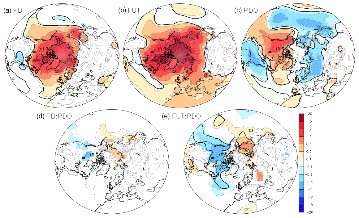
Figure 3 Surface air temperature at 2 m (in ^∘C) in response to sea-ice loss and PDO in the coupled simulations when using an analysis of the covariance: (a) effect of the PD sea-ice loss (β_PD in Eq. 2), (b) effect of the FUT sea-ice loss (β_FUT in Eq. 2), (c) effect of a warm PDO (β_PDO in Eq. 2), (d) effect of the interaction between PD sea-ice loss and the PDO (β_PD:PDO in Eq. (2), and (e) effect of the interaction between the FUT sea-ice loss and the PDO (β_FUT:PDO in Eq. 2). The color shades indicate a p value below 10 %. The black line indicates field significance, as given by the false discovery rate.

Arctic sea-ice loss additionally induces a significant deepening of the Aleutian Low and a negative NAO-like response. This is shown by the negative sea level pressure anomalies over the northern Pacific and central Atlantic, together with positive sea level pressure anomalies from Greenland to Norway (Fig. 4, top left and top center), with larger and broader anomalies in FUT than in PD. The geopotential height at 500 hPa (Fig. 5, top left and top center) also shows a strong increase over the polar cap in response to sea-ice loss. It increases above Greenland by as much as 20 m in PD and 40 m in FUT, which is consistent with the surface warming and the associated increase of the lower-tropospheric thickness. A negative AO pattern is also found: the geopotential height at 500 hPa decreases by approximately 15 m over a band from western North America to the Iberian Peninsula. Melting Arctic sea-ice also induces a small but significant deepening of the Aleutian Low at 500 hPa. In the stratosphere, the geopotential at 50 hPa increases over the polar cap in both FUT and PD cases and slightly decreases over southern Europe for PD and over northern Europe for FUT (Fig. 6, top left and top right). Figure 7 (top left and top right) further shows the zonal-mean zonal-wind changes, with a significant weakening of the poleward flank of the eddy-driven jet and of the polar vortex between 50 and 70^∘ N due to sea-ice loss. Between 30 and 40^∘ N the zonal wind is intensified from the surface to 70 hPa, at the core of the subtropical jet. The zonal wind also decreases south of 20^∘ N, in line with a shrinking of the subtropical jet.

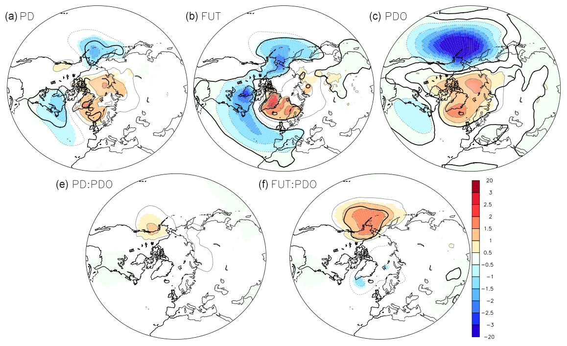
Figure 4 Same as Fig. 3 but for sea level pressure, in hectopascals (hPa).

The experiments can also be used to investigate the influence of a positive PDO on the atmosphere. A warm PDO induces a significant positive Pacific–North American (PNA)-like pattern, with a strong strengthening of the Aleutian Low, a ridge over northwestern North America/polar cap, and a small geopotential height increase over southeastern North America (Figs. 4 and 5, top right). Such impacts are consistent with the influence of the warm equatorial Pacific SST anomalies associated with the PDO onto the PNA (Trenberth and Hurrell, 1994; Newman et al., 2016). In the stratosphere, the geopotential height at 50 hPa shows a tripole pattern with a high over the Arctic and two lows over the eastern North Pacific and Europe, resembling the negative phase of the Arctic Oscillation (Fig. 6, top right). The warm PDO induces a significant weakening of the poleward flank of the eddy-driven jet from 50 to 70^∘ N, as well as a weakening of the stratospheric polar vortex between 50 and 80^∘ N (Fig. 7, top right). The zonal winds show a large increase between 20 and 40^∘ N at the core of the subtropical jet. Hence, if the PDO and the Arctic sea-ice loss impacts are considered to be additive, a warm PDO would enhance the Arctic sea-ice loss teleconnections in both the troposphere and stratosphere. Such PDO impacts are consistent with findings linking the PDO to the stratosphere based on observations (Woo et al., 2015) and models (Hurwitz et al., 2012; Kren et al., 2016). Nevertheless, it remains unclear whether the stratospheric impacts of the PDO are linked to the extratropical part of the PDO pattern or to the associated equatorial SST anomalies. Indeed, warm equatorial SST anomalies associated with an El Niño have been previously shown to drive a weakening of the Aleutian Low, which leads to decreased momentum flux from upward-propagating planetary waves that weaken the stratospheric polar vortex (Manzini et al., 2006; Hurwitz et al., 2012; Woo et al., 2015; Kren et al., 2016; Domeisen et al., 2019), a response that is consistent with our regression result for the PDO.

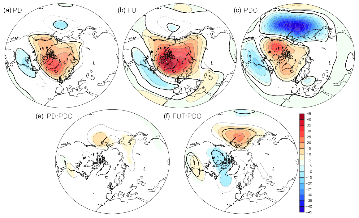
Figure 5 Same as Fig. 3 but for geopotential height at 500 hPa, in meters (m).

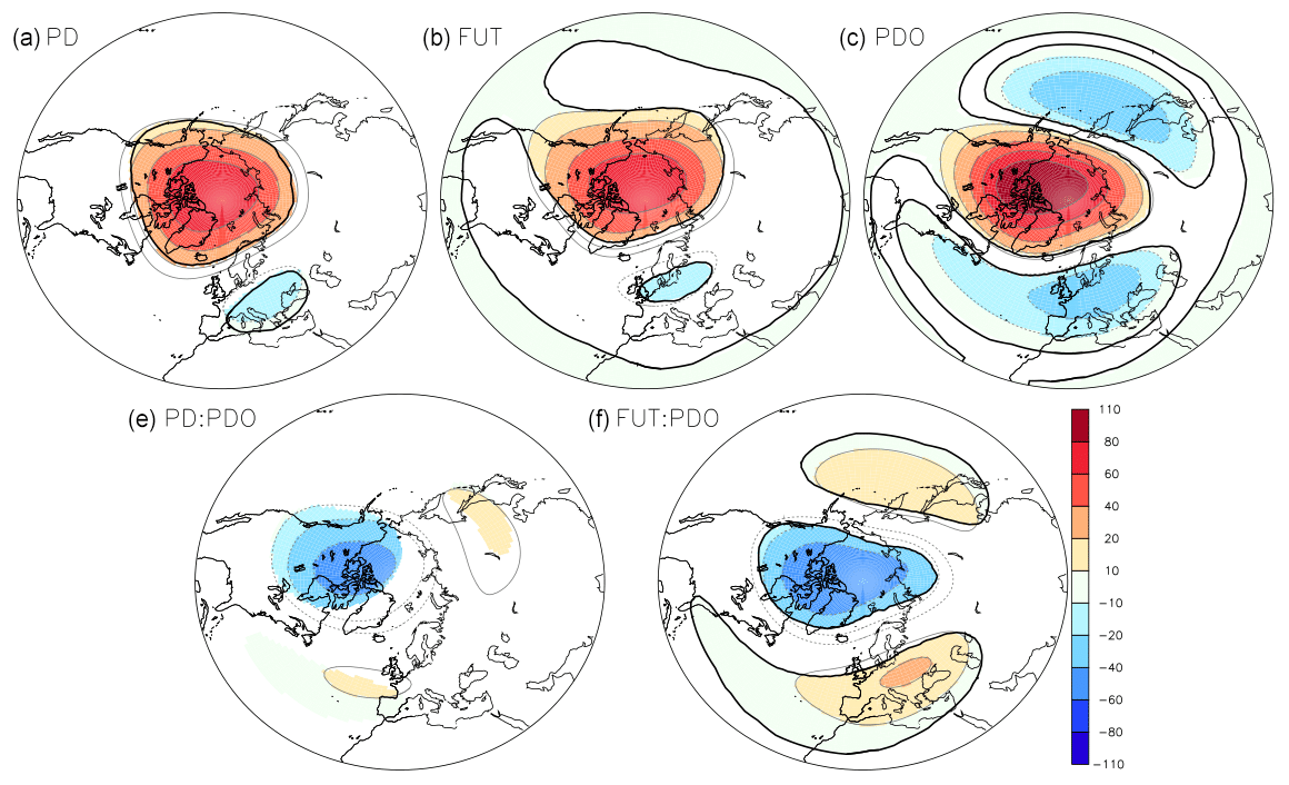
Figure 6 Same as Fig. 3 but for geopotential height at 50 hPa, in meters (m).

The interaction between sea-ice loss and the PDO leads to a weakening of the Aleutian Low (Fig. 4, bottom) and a pattern reminiscent of a wave train at 500 hPa, resembling a negative PNA phase (Fig. 5, bottom). The results of the interaction between sea-ice loss and PDO are qualitatively robust regardless of the magnitude of sea-ice loss (e.g., FUT or PD), but the amplitude of the interaction is small, and it is only significant in FUT. In PD, the interaction shows local p values below 10 % but is not field significant. Also, the effect of interaction is stronger and more significant in the stratosphere. At 50 hPa, a significant strengthening of the polar vortex is found, with negative anomalies above the polar cap and positive anomalies over the northwest Pacific and Europe (Fig. 6, bottom). Again, the stratospheric polar vortex increase is stronger and more significant for FUT than for PD. The interaction between PDO and sea-ice loss also shows zonal-wind changes consistent with a strengthening of the polar vortex (Fig. 7, bottom). Hence, the PDO and sea-ice loss impacts are not additive. The non-additive effect is given by the interaction term, with a reduction of the PDO and sea-ice loss teleconnections in both troposphere and stratosphere, in particular in the stratosphere.

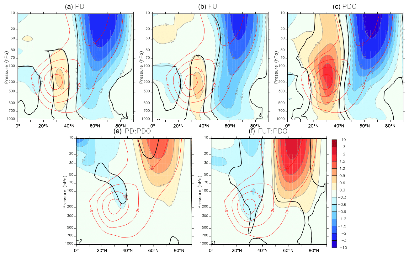
Figure 7 Same as Fig. 3 but for zonal-mean zonal winds, in meters per second (m s⁻¹). The black line indicates a p value below 10 %.

To understand the causes of the zonal-mean wind changes, the zonal-mean diagnostics of transformed Eulerian mean quantities are derived following Andrews et al. (1987). In response to FUT sea-ice melting, the warming located north of 40^∘ N is amplified toward the surface in the lower troposphere but extends throughout the troposphere (Fig. 8, top left). There is also important warming in the stratosphere from 100 to 10 hPa over the polar cap, north of 60^∘ N. The troposphere also warms between 20 and 30^∘ N, which can be linked to the shrinking of the subtropical jet (see Fig. 7). A warm PDO phase also leads to stratospheric warming (Fig. 8, top right) and a polar vortex weakening (Fig. 7, top right). However, it is associated with a warming of the tropical troposphere that is intensified in the upper troposphere. The warming over the Arctic associated with a positive PDO is rather uniform and is not intensified at the surface. A quasi-barotropic cooling is also located at 40^∘ N.

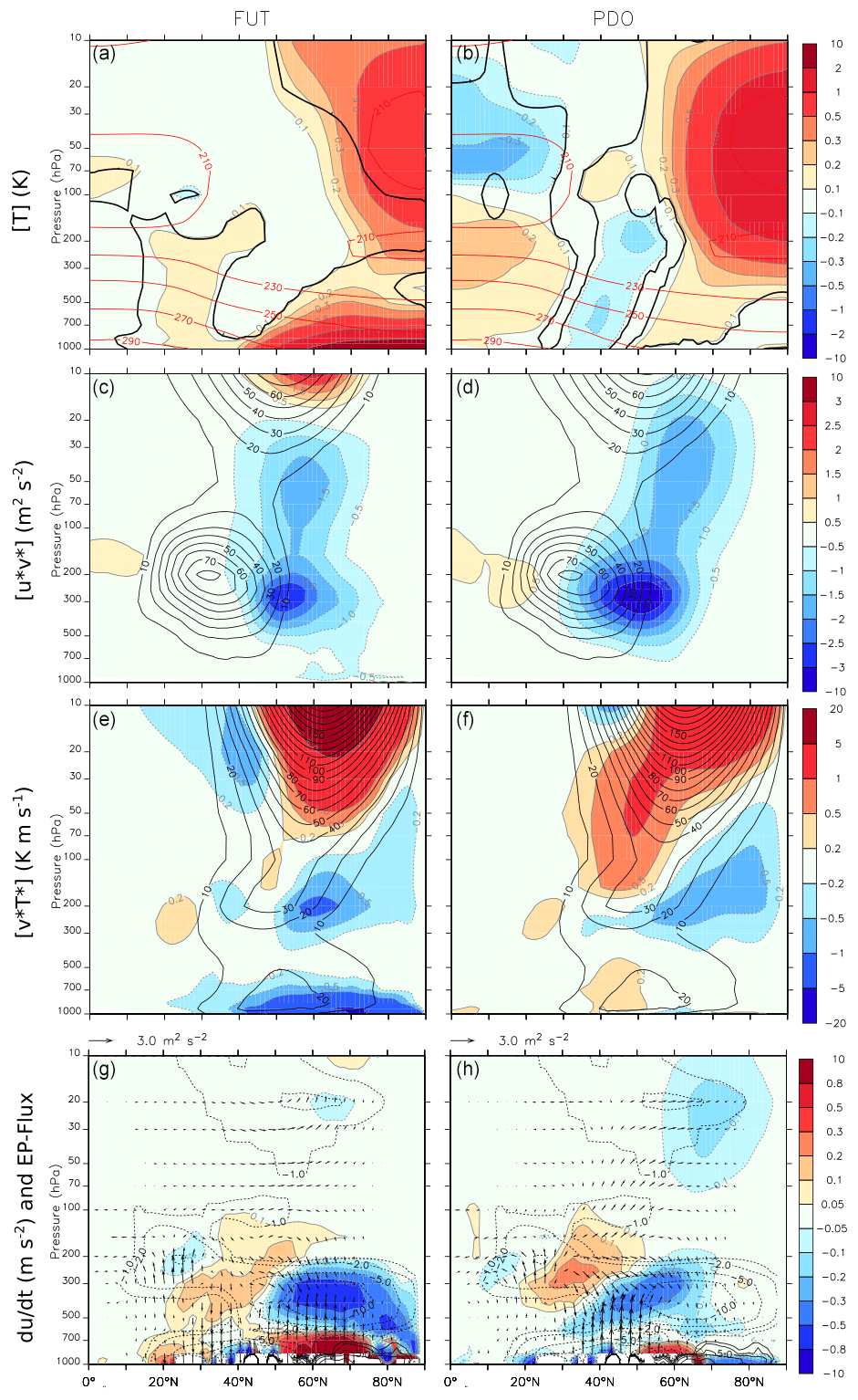
Figure 8 Zonal-mean temperature and atmospheric circulation changes related to (left panels) sea-ice loss in FUT and (right panels) PDO. Temperature (in K; first row), eddy momentum flux ($u^{*}{v}^{*}$ in m² s⁻²; second row), eddy heat flux ($v^{*}{T}^{*}$ in K m s⁻¹; third row), zonal-wind tendency implied by the Eliassen–Palm flux divergence (in 10² m s⁻¹ d⁻¹; bottom row, color shade) and Eliassen–Palm flux (m² s⁻²; bottom row, vectors). In the bottom row, the black contours show the zonal-wind tendency implied by the Eliassen–Palm flux divergence in the PI ensemble, chosen as a reference. The regressions with a p value below 10 % are indicated by a thick black line in the top panel.

Both sea-ice loss and PDO lead to a reduced eddy momentum flux at the poleward flank of the subtropical jet peaking around 300 hPa and extending into the stratosphere (Fig. 8, second row). The eddy heat flux (third row) weakens at the lower troposphere in response to sea-ice loss. In addition, both sea-ice loss and warm PDO decrease the eddy heat flux between 50 and 80^∘ N in the lower stratosphere at 200 hPa while increasing it above 100 hPa. The anomalous Eliassen–Palm (EP) flux is shown in Fig. 8 (bottom row; vectors), as well as the zonal-wind acceleration implied by the EP flux divergence (bottom row; shading). In normal conditions, the EP flux is directed upward and equatorward (not shown), and it converges into the upper troposphere, with two local maximums (Fig. 8, bottom row; contours). One maximum is located at 25^∘ N 200 hPa, while the other maximum is between 55 and 75^∘ N at 400 hPa. This convergence acts to decelerate the zonal wind. The FUT sea-ice loss reinforces the convergence between 55 and 75^∘ N at 400 hPa, with an anomalous upward EP flux in the lower troposphere below (Fig. 8, bottom; color shade). We verified that the convergence is due to the vertical component of the EP flux, which is proportional to the ratio between the eddy heat flux and the stratification. As the meridional eddy heat flux shows negative anomalies in this region, the intensification of the upward heat flux in 55–75^∘ N mainly results from the weaker atmospheric stratification, leading to a more unstable atmosphere. Between 30 and 40^∘ N, the EP flux is instead oriented downward in the troposphere, which leads to anomalous divergence between 500 and 200 hPa. It corresponds to the intensification of the core of the subtropical jet in Fig. 7 (top center). This change is again dominated by the vertical component of the EP flux (not shown) and might reflect the weakening of the meridional eddy heat flux. The same analysis for the PDO influence shows EP flux anomalies somehow similar to those associated with sea-ice loss. However, the intensification of the EP flux convergence is located between 40 and 60^∘ N, and the EP flux upper-tropospheric divergence at 30^∘ N is more intense. These changes are again associated with the vertical component of the EP flux (not shown) associated with an intensification of the tropospheric meridional eddy heat flux between 30 and 40^∘ N. In both sea-ice loss and PDO cases, the changes in the eddy momentum flux can be described as a positive feedback reinforcing the changes of the eddy heat flux, as in Smith et al. (2022). In the stratosphere, a clear intensification of the EP flux is simulated poleward and upward in response to sea-ice loss and PDO, consistent with the weakening of the polar vortex.

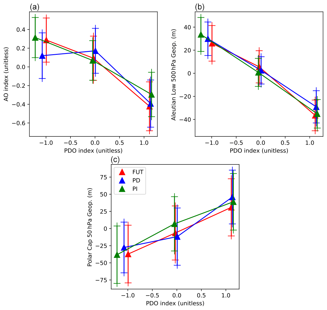
Figure 9 Composites of the AO index (a; unitless), Aleutian Low (b; in m) and polar cap 50 hPa geopotential height (c, in m), for members sorted following their PDO index in the PI (green lines), PD (blue lines) and FUT (red lines) ensembles. The dashed lines show the regression lines of the corresponding ensemble. The triangles indicate the value for each composite, constructed using PDO < $Q_{\mathrm{1}/\mathrm{3}}$, $Q_{\mathrm{1}/\mathrm{3}}$ < PDO < $Q_{\mathrm{2}/\mathrm{3}}$ and PDO > $Q_{\mathrm{2}/\mathrm{3}}$, where the threshold are given by $Q_{\mathrm{1}/\mathrm{3}}=-\mathrm{0}$.43 and $Q_{\mathrm{2}/\mathrm{3}}=\mathrm{0}$.43, the first and second tercile of a standard normal distribution. The error bar provides the 95 % confidence interval. The AO index is calculated as the first principal component of the 500 hPa geopotential height using all the members. The Aleutian Low index is the anomaly of the 500 hPa geopotential height in 40–50^∘ N, 150–180^∘ E. The polar cap 50 hPa anomalies is calculated with the mean value of the 50 hPa geopotential north of 60^∘ N.

4 Summary and discussion

We performed sensitivity experiments with the IPSL-CM6A climate model to study the short-term response (within 14 months) to the Arctic sea-ice loss. We focused on the winter (DJF) atmospheric circulation changes and how the PDO interacts with sea-ice impacts. The simulations show a robust negative NAO-like pattern in response to sea-ice melting, in line with most studies (Deser et al., 2015; Blackport and Kushner, 2016, 2017; McCusker et al., 2017; Oudar et al., 2017; Screen et al., 2018; Sun et al., 2018; England et al., 2020; Simon et al., 2021; Hay et al., 2022). A positive PNA with a strong deepening of the Aleutian Low is simulated in response to warm PDO, which is a well-established teleconnection (Trenberth et al., 1998; Mantua and Hare, 2002; Li et al., 2007). The response to Arctic sea-ice loss also includes a modest deepening of the Aleutian Low, as in Blackport and Screen (2019). The discrepancy with other studies in sign (Cjivanovic et al., 2017; Simon et al., 2021) or in amplitude (Screen et al., 2018; Hay et al., 2022) can be explained by the timescale investigated. Both Blackport and Screen (2019) and our study are focused on short response timescales of less than 5 years, which might be too short to affect the trade winds and generate SST anomalies in the tropics. Sea-ice melting and the PDO were found to generate similar atmospheric circulation changes. Both lead to a weakening of the eddy-driven jet on its poleward flank, an intensification of the subtropical jet and a weakening of the polar vortex. However, for sea-ice loss, these changes are governed by the lower-tropospheric warming north of 50^∘ N and the weaker lower-tropospheric meridional temperature gradient. The weakening of the eddy-driven jet on its poleward flank is induced by weaker surface stratification leading to an increased upward Eliassen–Palm flux and acting to reduce the mean zonal flow. Conversely, we show that a warm PDO phase mainly intensifies the Aleutian Low and the transient eddy heat flux at 30–40^∘ N into the stratosphere. The wintertime tropospheric stationary wave deepens during strong Aleutian Low, which is known to lead to a weakening of the polar vortex (Nakamura and Honda, 2002; Garfinkel et al., 2010; Smith et al., 2010). The combined response of the midlatitude atmospheric circulation to a warm PDO and sea-ice melting is not additive, with the interaction between both signals being partly destructive. For reduced sea-ice extent and a warm PDO phase, the impacts are smaller than the ones expected by the addition of the two effects. This applies to the anomalies simulated in both the troposphere and stratosphere. The overall results agree with Screen and Francis (2016), with sea-ice loss contribution to Arctic amplification being modulated by PDO. However, their results indicate that Arctic warming in response to the ongoing long-term sea-ice decline is smaller during warm PDO phases. The framework proposed here assesses that the additional effect of the Arctic sea-ice loss and warm PDO enhances the Arctic sea-ice teleconnections while the non-additive effect, linked to the atmospheric circulation in the stratosphere, reduces them. Screen and Francis (2016) used sea-ice loss and PDO forcings larger than the ones investigated here. They found slightly larger responses than ours in the near-surface temperature or zonal winds. We also found a broader near-surface temperature increase over the Arctic due to sea-ice loss and a broader PDO response in the North Pacific.

Figure 10 Difference between the 200-member ensemble of FUT and PI (color and gray outline) in DJF for the geopotential height at 500 hPa (m; top), the geopotential height at 50 hPa (m; middle top), the zonally averaged zonal wind (m s⁻¹; middle bottom), and the zonally averaged temperature (K; bottom) in the coupled (left) and atmosphere-only (right) configurations of the IPSL-CM6A-LR. Colors are masked if the confidence level of the Student t test is less than 90 %. The 90 % confidence level based on the false discovery rate (FDR) is given in black contours for the two top rows. On the middle bottom and bottom panels, the zonal mean of the wind zonal of the PI simulation in DJF is indicated by the red contours with an interval of 5 m s⁻¹, the thick red line indicates zero, the solid line indicates positive values and the dashed line indicates negative values.

The general linear model presented here can be applied to the analysis of other modes of climate variability or ensembles of sensitivity experiments, such as the idealized experiments of the DCPP (Decadal Climate Prediction Project) panel of CMIP6. The model uses all the ensemble members when estimating the different influences, which are thus based on a larger sample than in traditional methods, and it does not involve the choice of an arbitrary threshold, as when building composites. However, the method does not account for non-linearities, and the impacts of warm and cold PDO could be asymmetric. Therefore, we performed a composite analysis by averaging members of the PI, PD and FUT ensemble for warm, neutral and cold phases of the PDO. The composites are built using members with a PDO index lower than −0.43 (cold phase), between −0.43 and 0.43 (neutral phase), and higher than 0.43 (warm phase). The thresholds of −0.43 and 0.43 correspond to the first and second tercile of the standard normal distribution. For Gaussian climate indices, this leads to a composite of approximately the same size. We found that the changes of the AO, Aleutian Low and the polar vortex are symmetric in most of the composites (Fig. 9). The AO pattern is only slightly asymmetric in the present-day sea-ice conditions, as the neutral and cold PDO states have a similar AO impact (Fig. 9; top left). This is also the case for the polar vortex anomalies in FUT (Fig. 9; bottom). Hence, the linear analysis seems applicable to a good approximation.

Observational studies estimate that winter Arctic sea-ice loss could have led to a much larger NAO-like anomaly than the one found here, with as much as 200 m over Iceland at 500 hPa over the last four decades if linearity and perpetual winter conditions could be assumed (Simon et al., 2020). Nonetheless, the Arctic sea-ice loss impact on the NAO is smaller in our sensitivity experiments (30 to 50 m). The reasons for this discrepancy are under active debate (Cohen et al., 2020). Although the effect of the surface sea-ice condition is weak (Smith et al., 2022), this lack of sensitivity in models might contribute to explain the much too weak persistence of climate variability in models. This deficiency might stem from the so-called signal-to-noise paradox in seasonal-to-decadal climate prediction systems (Scaife et al., 2014; Scaife and Smith, 2018; Zhang and Kirtman, 2019; Smith et al., 2020), which remains to be solved. The discrepancy might be explained by too weak eddy feedback represented in models (Smith et al., 2022) but also by the difficulty to cleanly attribute a response to Arctic sea-ice decline in observations. Here, we show that the PDO is an important concomitant factor that has an impact on the Arctic similar to that of Arctic sea-ice loss, especially in the stratosphere. Much care is therefore needed to separate these two effects when using observations. The analysis presented in this paper could be repeated in a multi-model framework to investigate the robustness of these conclusions, such as through PAMIP simulations. For this, it is important to keep in mind that depending on the protocol used to constrain sea ice in coupled model sensitivity experiments, the amplitude of the atmospheric response to sea-ice loss can vary by a factor of 2 (Simon et al., 2021). Moreover, sea-ice thickness was not constrained in the sensitivity experiments but might play an important role in the atmospheric circulation response (Lang et al., 2017). Great caution is therefore required when interpreting the results of different models using different ice-constraining methods.

The bulk of our analysis was based on simulations with an ocean–atmosphere general circulation model. However, a different response to sea-ice loss might be obtained with atmospheric-only configurations where the two-way air–sea coupling is not allowed. Studies have primarily investigated the ocean feedback on timescales from decadal to centennial. Deser et al. (2015) found that full ocean coupling amplifies the Arctic sea-ice loss impact in 100-year simulations, while no feedback was found in an atmospheric model coupled to a slab ocean at decadal timescales in Cvijanovic et al. (2017). However, few studies have investigated short simulations of 14 months, where only fast feedbacks can operate. To determine the role of the coupling, we have performed the same sensitivity experiments but using the atmosphere-only configuration of the IPSL-CM6A-LR model (hereafter ATM). We find that the tropospheric circulation response to sea-ice loss is very similar to that in the coupled experiments, although the increase of the 500 hPa geopotential height over the Arctic is weaker in the ATM model (Fig. 10, top). Moreover, the coupled simulations present a stronger weakening of the stratospheric polar vortex than the atmospheric-only simulations (Fig. 10, middle rows). The lower-troposphere warming is more intense in the coupled model and extends more upward, which reflects the presence of sea-ice–ocean–atmosphere feedbacks, such as those involving thinner sea ice. The eddy heat flux reduction also extends more toward the tropics in the coupled runs compared to the atmosphere-only simulations (Fig. S2, bottom left). Both changes intensify the subtropical jet at 30^∘ N and are associated with intensified upward propagation of planetary waves into the stratosphere (compare Fig. 8 bottom left to Fig. S2 bottom right), which might explain the reduction of the stratospheric polar vortex in the coupled experiments. Since the tropospheric response to a weakened polar vortex resembles the negative AO (Baldwin and Dunkerton, 1999; Kidston, 2015; Cohen et al., 2017; Hoshi et al., 2019), the stronger stratospheric polar vortex weakening might explain the larger AO anomaly in the coupled experiments.

We applied the same analysis as for the PDO to investigate the AMV, defined as the SST over the box 0–60^∘ N, 0–80^∘ W; the influence; and its modulation by sea-ice loss in the sensitivity experiments with the coupled model, similarly using its distribution among members resulting from the different initial North Atlantic conditions. It was further applied to the QBO defined as the equatorial zonal wind at 30 hPa. In both QBO and AMV cases, their identified impacts onto the atmospheric circulation were barely significant, and there was no significant interaction with sea-ice loss (see Fig. S1, bottom).

The ocean changes were not investigated in these short simulations, as they are likely to be small and confined to the surface mixed layer. However, sea-ice loss impacts on the ocean could be very different in longer simulations. Indeed, the atmospheric response to sea-ice loss can be different in transient (a few decades) or equilibrium conditions (more than five decades) (Simon et al., 2021; Blackport and Kushner, 2016; Liu and Fedorov, 2019). In particular, the changes in the Beaufort Gyre (Lique et al., 2018), North Atlantic inflow (Simon et al., 2021), subpolar North Atlantic (Hay et al., 2022) and Atlantic Meridional Oceanic Circulation (Sévellec et al., 2017) would play an important role.