the Creative Commons Attribution 4.0 License.
the Creative Commons Attribution 4.0 License.
 | 04 Aug 2022
Diabatic processes modulating the vertical structure of the jet stream above the cold front of an extratropical cyclone: sensitivity to deep convection schemes
Gwendal Rivière
Philippe Arbogast
Jean-Marcel Piriou
Julien Delanoë
Carole Labadie
Quitterie Cazenave
Jacques Pelon
The effect of deep convection parameterisation on the jet stream above the cold front of an explosive extratropical cyclone is investigated in the global numerical weather prediction model ARPEGE, operational at Météo-France. Two hindcast simulations differing only in the deep convection scheme used are systematically compared with each other, with (re)analysis datasets and with NAWDEX airborne observations.
The deep convection representation has an important effect on the vertical structure of the jet stream above the cold front at 1-d lead time. The simulation with the less active scheme shows a deeper jet stream, associated with a stronger potential vorticity (PV) gradient in the middle troposphere. This is due to a larger deepening of the dynamical tropopause on the cold air side of the jet and a higher PV destruction on the warm air side, near 600 hPa. To better understand the origin of this stronger PV gradient, Lagrangian backward trajectories are computed.
On the cold air side of the jet, numerous trajectories undergo a rapid ascent from the boundary layer to the mid-levels in the simulation with the less active deep convection scheme, whereas they stay at mid-levels in the other simulation. This ascent explains the higher PV noted on that side of the jet in the simulation with the less active deep convection scheme. These ascending air masses form mid-level ice clouds that are not observed in the microphysical retrievals from airborne radar-lidar measurements.
On the warm air side of the jet, in the warm conveyor belt ascending region, the Lagrangian trajectories with the less active deep convection scheme undergo a higher PV destruction due to a stronger heating occurring in the lower and middle troposphere. In contrast, in the simulation with the most active deep convection scheme, both the heating and PV destruction extend further up into the upper troposphere.
- Article
(14003 KB) - Full-text XML
-
Supplement
(2537 KB) - BibTeX
- EndNote


Midlatitude high-impact weather (HIW) events are usually dynamically forced by near-tropopause disturbances and by specific configurations of the jet stream. Their surface imprints largely depend on the structure and intensity of the jet stream aloft. For instance, the rapid deepening of wind storms depends on the intensity of the jet stream (Wernli et al., 2002; Pinto et al., 2009; Rivière et al., 2010) and is favoured by the presence of a jet streak (Uccelini, 1990; Fink et al., 2009). As a second example, heavy precipitation and flood events are often forced by an elongated trough along the jet stream or a cut-off that just separated from the jet stream following wave breaking (Massacand et al., 1998; Martius et al., 2008; Nuissier et al., 2011; Grams et al., 2014). Since the near-tropopause disturbance triggering the HIW event is often part of a Rossby wave train, the skill of numerical weather prediction (NWP) models to accurately predict a HIW event depends on their ability to represent the troughs and ridges propagating along the jet stream during the days prior to the event (Parsons et al., 2017; Wirth et al., 2018). Consequently, there is a growing body of literature identifying systematic NWP biases along these downstream propagating near-tropopause wave-like disturbances (Rodwell et al., 2013; Gray et al., 2014) and investigating dynamics of forecast errors along the midlatitude waveguide (Davies and Didone, 2013; Baumgart et al., 2018).
Looking at different NWP models, Gray et al. (2014) found systematic forecast errors in the jet representation increasing with forecast lead times. In particular, the potential vorticity (PV) gradient becomes smoother on the poleward flank of ridges and Rossby wave amplitudes get smaller, the two being closely related (Harvey et al., 2016). Another consequence of the too smooth PV gradient is the slowdown of phase speed with forecast lead time (Harvey et al., 2018). It is in that particular context that the international field campaign NAWDEX (North Atlantic Waveguide Downstream Impact EXperiment) occurred in September–October 2016 (Schäfler et al., 2018). The objective of NAWDEX was to investigate the diabatic origin of forecast errors in the ascending part of extratropical cyclones along the so-called warm conveyor belts (WCBs), to analyse their downstream propagation along the waveguide and how they may affect the predictability of HIW events. Using NAWDEX observations as a reference, Schäfler et al. (2020) showed underestimation of vertical wind shear in the vicinity of the tropopause in very short-term forecasts (up to 10 h) and analysed that this could affect Rossby wave propagation by altering the strength of the PV gradient.
Regions of strongest forecast errors and systematic analysis of forecast busts suggest that forecast errors originate from diabatic processes (Rodwell et al., 2013; Gray et al., 2014). Because of the PV invertibility properties and its conservation under adiabatic and frictionless processes, the PV perspective offers a classical and useful framework to investigate the influence of diabatic processes on the atmospheric flow. The PV tracer technique that decomposes the PV rate of change into different model processes has been widely used during the last decade, mainly to study the near-tropopause PV anomalies associated with the jet stream (Chagnon et al., 2013; Martinez-Alvarado et al., 2014; Saffin et al., 2017; Spreitzer et al., 2019; Harvey et al., 2020). Such a technique has also been used to study low-level PV anomalies associated with extratropical cyclones (Crezee et al., 2017; Attinger et al., 2021).
The former cited studies found that near-tropopause PV is strongly affected by diabatic processes, mainly by latent heating, turbulence and longwave radiation, and these processes maintain the strong PV gradient there. Saffin et al. (2017) showed that the decrease in tropopause sharpness with forecast lead time, originally diagnosed by Gray et al. (2014), is mainly due to the advection scheme and is only partially compensated by the increase in tropopause sharpness due to nonconservative processes.
The PV and potential temperature (θ) Lagrangian framework in general, can also be used to explain atmospheric circulation (Chagnon et al., 2013; Crezee et al., 2017; Spreitzer et al., 2019; Harvey et al., 2020) differences between simulations performed with distinct models (Martinez-Alvarado et al., 2014) or between sensitivity numerical experiments made with the same model but using different parameterisation schemes (Martinez-Alvarado and Plant, 2014; Joos and Forbes, 2016; Mazoyer et al., 2022; Rivière et al., 2021).
Joos and Forbes (2016) and Mazoyer et al. (2022) used this approach to analyse the sensitivity of jet stream structure and WCB to distinct cloud microphysics schemes at 2–3 d lead times. Both found some effects of the microphysics representation on the WCB and the tropopause position along the edge of the ridge building, using the ECMWF-IFS global model in Joos and Forbes (2016) and using a regional convection permitting model in Mazoyer et al. (2022).
The PV-θ framework has been also used to analyse WCB differences and impact on the tropopause with different deep convection parameterisation schemes (Martinez-Alvarado and Plant, 2014; Rivière et al., 2021) but the amplitude of the impact on the upper-level circulation varies from case to case. Martinez-Alvarado and Plant (2014) found relatively modest differences in the tropopause location after 24 h for a moderate cyclone between reduced and intense parameterised convection, while Rivière et al. (2021) found important differences with a jet stream shift of a few hundred kilometers after 24 h for an explosive cyclone.
Recent NAWDEX-related studies have emphasised the importance of embedded convection within WCBs by comparing satellite observations and convective-permitting simulations to airborne radar measurements gathered during NAWDEX (Oertel et al., 2019, 2020, 2021; Blanchard et al., 2020, 2021). Oertel et al. (2020) and Blanchard et al. (2021) showed that the heating associated with embedded convection generates a PV dipole near the tropopause that reinforces the PV gradient and hence the jet stream. The ability of convectively created PV dipole to reinforce the jet depends on the region where convection occurs and on the vertical wind shear (Chagnon and Gray, 2009; Harvey et al., 2020; Oertel et al., 2021).
Following the same approach as in a companion paper (Rivière et al., 2021, hereafter RW21), the present study investigated the effect of parameterised deep convection on WCB and jet stream. RW21 compared three simulations of the Météo-France global model ARPEGE: two simulations were performed with two distinct deep convection parameterisation schemes developed within ARPEGE, the one described in Bougeault (1985, thereafter B85) and the prognostic condensates microphysics and transport scheme of Piriou et al. (2007, hereafter PCMT). The third simulation was performed without any deep convection parameterisation.
Without deep convection parameterisation the heating ahead of the cold front is organised in distinct cells of high values with a few degrees extent in longitude and latitude because convective instability is released at the resolved scales. In contrast, in presence of parameterised deep convection, the heating is much smoother because convective instability is released at subgrid scales. The consequence is that WCB ascents are more sustained with parameterised deep convection, while they are more abrupt without. This regulating effect of deep convection parameterisation on WCB was already noticed by Martinez-Alvarado and Plant (2014). However, this does not mean that the impact on the tropopause is stronger without deep convection parameterisation. RW21 showed that the run in which deep convection is more active (namely, the simulation with B85) is also the one for which the total heating (from all parameterisation) extends further upward above the warm front of the extratropical cyclone and has a stronger PV destruction at upper levels. This leads to a shift of the jet stream of about 100 km to the west compared to the other two runs, the one with PCMT deep convection scheme and the other without any active scheme. In addition, a clear dependence of the jet stream structure on the closure of the deep convection scheme has been noticed in the WCB outflow region.
In RW21, the focus was on the WCB outflow region above the bent back warm front and the horizontal structure of the jet stream, while in the present study, the focus is on the WCB ascending region above the cold front. As in RW21, the aim is to analyse differences between the same three simulations and in contrast to the previous study, to highlight differences in the vertical structure of the jet stream.
The extratropical cyclone hereafter studied, called the Stalactite cyclone (1–4 October 2016), is of particular interest in a number of aspects. It was formed off the Newfoundland coast and intensified over the North Atlantic with a deepening rate of 24 hPa in 24 h (Flack et al., 2021) as a classical bomb event (Sanders and Gyakum, 1980). It has been intensively observed during NAWDEX (Schäfler et al., 2018) by three flights: two flights of the French Falcon 20 from the Service des Avions Français Instrumentés pour la Recherche en Environnement (SAFIRE) and one flight from the Deutsches Zentrum für Luft- und Raumfahrt (DLR) Dassault Falcon. Its development was accompanied by a burst in latent heating (Steinfeld et al., 2020) and the ridge building aloft led to the onset stage of the “Thor” block (Maddison et al., 2019) that lasted until the end of NAWDEX in mid-October 2016.
The paper is organised as follows. Section 2 presents the data and methods. It includes the description of the model simulations and the main characteristics of the two deep convection schemes B85 and PCMT. It also provides information on various (re)analysis datasets and on airborne observations made during the flight of the SAFIRE Falcon aircraft on 2 October over the ascending WCB region of the Stalactite cyclone. Finally, Sect. 2 details the computation of PV-θ Lagrangian budgets. Section 3 shows differences in the jet stream representation between the different simulations and (re)-analysis datasets. Section 4 provides an explanation for these differences in terms of the PV-θ framework. Section 5 compares model simulations to airborne observations to highlight the more realistic forecasts in the different regions. Finally Sect. 6 is dedicated to the concluding remarks and discussion.
2.1 Model and simulation set-up
As in the companion paper RW21, the study relies on simulations of the operational Météo-France global model, Action de Recherche Petite Echelle Grande Echelle (ARPEGE Courtier et al., 1991) and in particular on different members of its associated ensemble prediction system, called Prévision d'Ensemble ARPEGE (PEARP, Descamps et al., 2015).
For all PEARP members, the vertical resolution has 90 levels while the horizontal grid corresponding to T798 resolution, is stretched by a factor of 2.4 and centred on France. Consequently, this resolution is about 10 km on France, 15 km on the zone of interest of this study and 60 km on the antipode of France. The time step of the model is 7.5 min. Model outputs are available with a temporal resolution of 15 min and a horizontal resolution of 0.5∘, while the vertical resolution is 50 hPa.
While operational PEARP members include perturbations in both model physics and initial conditions, the present study is based on PEARP reforecast dataset corresponding to 10 members that have the same initial conditions (ARPEGE operational 4D-Var analysis at 12:00 UTC 1 October 2016) and only differ in their physics as in Ponzano et al. (2020), Binder et al. (2021) and RW21.
Among the 10 members 2 are hereafter investigated more deeply. They only differ in their deep convection scheme: one with B85, the other with PCMT. They are referred as the REF and member 7 in Ponzano et al. (2020). In addition, a third simulation, called NoConv, has no deep convection scheme activated. For more details on these three simulations, particularly concerning physical parameterisation, the reader is referred to RW21.
2.2 Differences between the two deep convection schemes
The two simulations studied in the present paper use two distinct parameterisation schemes of deep convection, both being based on the mass-flux approach. Detrainment in the environment, precipitation and downdraft phenomena are modellised in both B85 and PCMT, but in contrast to B85, the PCMT scheme is able to estimate the prognostic mixing ratios of the different hydrometeors inside the mass flux (updraft). It includes the same four hydrometeors (liquid cloud water, pristine ice, rain and snow) involved in the large-scale cloud microphysical scheme of Lopez (2002), and the same microphysical phenomena, such as accretion, autoconversion, riming.
The two schemes are activated with two distinct closures. Bougeault's (1985) scheme is activated with the convergence of total moisture fluxes (including both resolved and turbulent moisture fluxes) integrated from the surface to the considered level and when the atmosphere presents an unstable profile. In contrast, the PCMT scheme considers a closure based on the convective available potential energy (CAPE).
2.3 Airborne observations and (re)analyses
To better compare the effects of the deep convection scheme and to better estimate their realism, two types of references are used: observations from the NAWDEX IOP6, as well as operational analyses and reanalysis.
2.3.1 Observations from NAWDEX IOP6
The flight of the French Falcon 20 of SAFIRE, studied in the present study, occurred between 13:01 and 16:16 UTC on 2 October during the NAWDEX field campaign (Schäfler et al., 2018). Figure 1 shows the position of the flight in relation to the Stalactite cyclone. The aircraft took off at Keflavik, went south, realised a clockwise loop triangular in shape to the northeast of the cyclone.
The major part of the flight occurred in the cloudy region ahead of the cold front close to the cyclone centre, which likely corresponds to the ascending part of the WCB (Fig. 1b) but the clear sky zone appearing near the westernmost vertex of the triangle suggests that the flight crossed the cold front from east to west near 58∘ N.
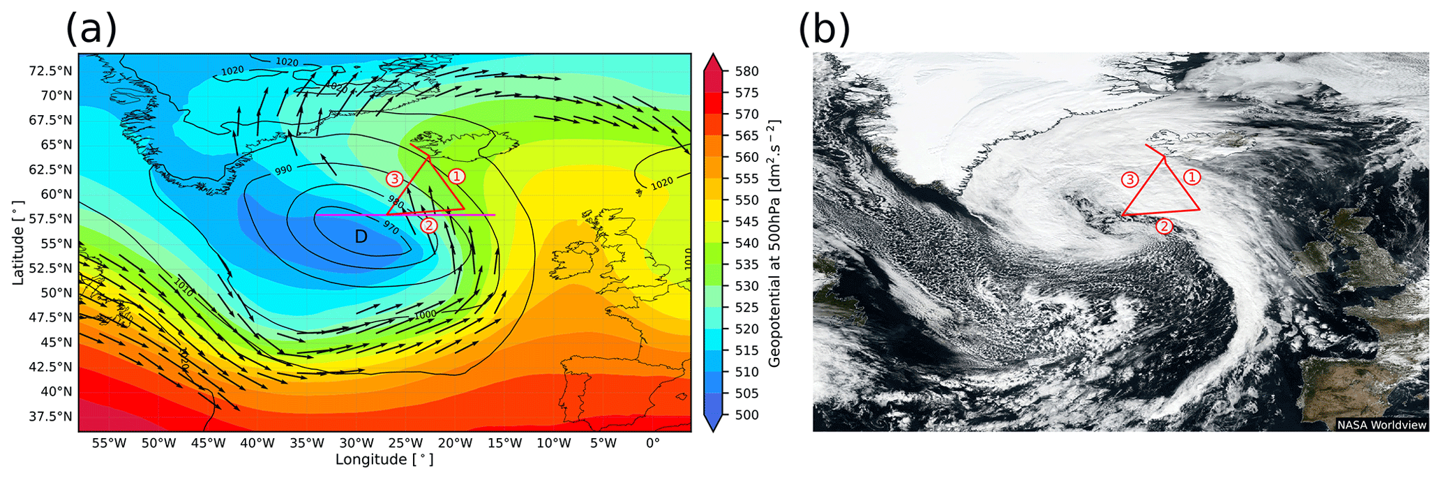
Figure 1Visualisation of the Stalactite cyclone during its mature stage on 2 October 2016. (a) Geopotential at 500 hPa (shading), sea level pressure (thin black contour) at 12:00 UTC, wind direction at 300 hPa for wind speed superior to 40 m s−1 (arrows), Falcon flight (bold red line) and vertical cross-section at 58∘ N (bold magenta line) (b) visible picture from VIIRS of the Suomi NPP satellite (NASA Worldview) with the Falcon flight in red.
In situ sensors on board the SAFIRE Falcon 20 measured pressure, wind and temperature at the flight level near 300 hPa. In addition, the RALI (RAdar-LIdar) platform was on board the aircraft. This platform includes a multi-beam 95 GHz Doppler cloud radar (RASTA, radar airborne system; Delanoe et al., 2013) and a Doppler high-spectral-resolution lidar (LNG; Bruneau et al., 2015). The RASTA measures both reflectivity and Doppler velocity along three non-collinear directions thanks to three downward antennas (nadir, backward and transverse). This configuration allows the 3D wind field to be retrieved in the vertical below the Falcon with a range resolution of 60 m and every 0.75 s leading to a horizontal resolution of about 300 m at the speed of the aircraft. The lidar operates at 532 and 1064 nm in backscatter mode only but measures Doppler velocity, polarisation and the backscattered light from molecules and particles separately at 355 nm. It gives information about optical parameters of aerosol and thin clouds together with wind below the aircraft at 15 m and 5 s range and time resolution, respectively. Additional wind measurements were also made by drop sondes.
To better compare observations with model outputs, in situ and RALI measurements have been averaged over intervals of 180 s as the Falcon 20 (with its mean speed of about 200 m s−1) travels, in that time, a distance of 36 km corresponding approximately to the horizontal grid spacing of the model outputs.
2.3.2 Operational analysis and reanalysis
The ERA5 reanalysis (Hersbach et al., 2018a) and operational analyses of the ARPEGE and integrated forecasting system (IFS) models are used at same vertical resolution of 50 hPa and horizontal resolution of 0.5∘ than the ARPEGE simulation outputs.
2.4 Lagrangian warm conveyor belt trajectories
2.4.1 Initialisation in the warm sector
The same forward trajectories as those shown in RW21 are used. They are initialised at 12:00 UTC on 1 October in the warm sector of the extratropical cyclone and last 48 h. These trajectories are seeded in a box from 50–20∘ W, 35–56∘ N and 1000–800 hPa, with a horizontal resolution of 0.5∘ and a vertical resolution of 20 hPa. To select WCB trajectories, a criterion of an ascent exceeding 300 hPa within 1 d during the period between 12:00 UTC on 1 October and 12:00 UTC on 3 October is applied. This is a less selective criterion than the more usual ascent of 600 hPa in 2 d but has the advantage of selecting a larger set of trajectories.
2.4.2 Initialisation along the flight
To better characterise properties of the WCB air masses of the Stalactite cyclone crossing the flight F7, another set of trajectories has been computed with the same trajectory algorithm as in RW21. It consists of 24 h backward and 24 h forward trajectories starting from the flight legs over the whole vertical axis. For each flight leg, the trajectories are seeded on a vertical regular grid spacing of 12.5 hPa from 975 to 200 hPa (63 seeding points on the vertical axis) and on a horizontal grid spacing of about 0.3∘ in longitude and latitude (84 seeding points on the horizontal axis, whose index, ordered according to flight travel, defines the trajectory index).
As the flight lasted more than 3 h, trajectories from each flight leg must be seeded at a different time. The time of seeding is the time when the aircraft is in the middle of each leg. Hence, the first leg trajectories are seeded at 26.25 h forecast range, namely 14:15 UTC on 2 October, the second leg trajectories at 27 h forecast range corresponding to 15:00 UTC and finally the third leg trajectories at 27.75 h forecast range, at 15:45 UTC.
Overall, 5292 trajectories lasting 48 h have been computed with 5292 seeding points along the flight path (63 in the vertical × 84 in the horizontal). To prevent trajectories crossing the surface, pressure is limited at 975 hPa. Trajectories with a minimum ascending rate of 300 hPa in 24 h are considered as belonging to the WCB. This leads to 1870 WCB trajectories for B85 and 1972 WCB trajectories for PCMT.
2.5 Heating and PV tendencies
As in RW21, the heating is computed in two different manners. The first method uses instantaneous temperature tendency datasets associated with the different diabatic processes parameterised in the model (large-scale cloud microphysics, convection, radiation, turbulence). These temperature tendencies are first provided on the ARPEGE stretched grid and model levels before being interpolated on the 0.5∘ × 0.5∘ horizontal grid and pressure levels. The second method computes the heating using centred finite-difference schemes applied to the potential temperature at the resolution of the model outputs chosen for this study: 0.5∘ × 0.5∘ in the horizontal, 50 hPa in the vertical and 15 min in time. Since the Lagrangian trajectories are also computed on the latter grid, the variations in θ along trajectories are very close to the integrated heating obtained with the second method (not shown). The first method only roughly approximates the variations in θ along trajectories for mainly two reasons: firstly, the dynamical core of ARPEGE does not strictly conserve θ because of numerical diffusion in the advection scheme and secondly the various interpolation steps in the offline trajectory algorithm to get the temperature tendency terms on the model output grid generate uncertainties. Both methods are hereafter used and information on the choice of the method is provided in the captions of the figures: the second method has the advantage to nearly close the heating budget while the first method has the advantage to provide a decomposition of the heating into various diabatic processes.
As the PV tendency depends on spatial variations of the heating and frictional terms (see Eq. 4 in RW21), their computation is made by applying finite-difference schemes to the heating and frictional terms. The frictional terms in the zonal and meridional momentum equations are available in the stretched and rotated Gaussian reduced model grid and at model levels. They are first interpolated on the 0.5∘ × 0.5∘ horizontal and 50 hPa vertical grids before applying the finite-difference schemes to them. The heating is computed following the second method described above as it leads to a much more accurate approximation of the total PV tendency than the first method.
The vertical structure of the jet stream at 58∘ N is shown for the three simulations and different (re)analysis datasets in Fig. 2. This latitude roughly corresponds to the southern leg of the flight (see grey line in Fig. 1a) and to the western edge of the upper-level ridge. In the three references (i.e. the two analyses and ERA5), the maximum wind speed is located near 24∘ W between 300 and 400 hPa at the interface between stratospheric and tropospheric air and varies between 55 and 60 m s−1. The height of maximum wind speed fluctuates from dataset to dataset with greater heights in the two analyses than in ERA5. Such differences in wind speed are accompanied by similar differences in PV: the dynamic tropopause (2 PVU isoline) descends until about 400 hPa in the two analyses while it descends further down to 500 hPa in ERA5. The jet stream is narrower and slightly deeper in ERA5 than in the analyses, consistent with stronger PV gradient between 400 and 500 hPa in the former than in the latter datasets. The three ARPEGE forecasts with distinct deep convection representation simulate the speed and position of the jet stream reasonably well in comparison with the three references: the jet stream is also centred at 24∘ W with a maximum between 50 and 60 m s−1 in both simulations. However, the vertical structure differs from one run to another. The PCMT and NoConv simulate a deeper jet stream with a centre located at 390 hPa with wind speed values up to 40 m s−1 reaching 650 hPa. In contrast, in B85, such high wind speed values do not go further down than 575 hPa. The deeper jet stream in PCMT and NoConv is associated with a lower tropopause to the west, going until 650 hPa in both PCMT and NoConv and only to 400 hPa in B85. It is associated with negative PV values going further down to the east until 525 hPa in PCMT and until 475 hPa in NoConv while it reaches higher altitude until 250 hPa in B85.

Figure 2Vertical cross-section at 58∘ N (grey line in Fig. 1) of the zonal wind (shadings) and potential vorticity (black contours with hatched areas for values superior to 2 PVU, bold contour for 0 PVU) at 15:00 UTC, 2 October 2016 for (a) ECMWF-IFS analysis, (b) ARPEGE analysis, (c) ERA reanalysis, (d) simulation with B85, (e) simulation with PCMT and (f) simulation without deep convection parameterisation. The thick crosses represent the location of wind speed maxima.
Table 1Root mean square of the difference with ERA5 reanalysis of the ECMWF-IFS and ARPEGE analyses and the three forecasts in PV and wind speed at 600 hPa over the domain shown in Fig. 3.
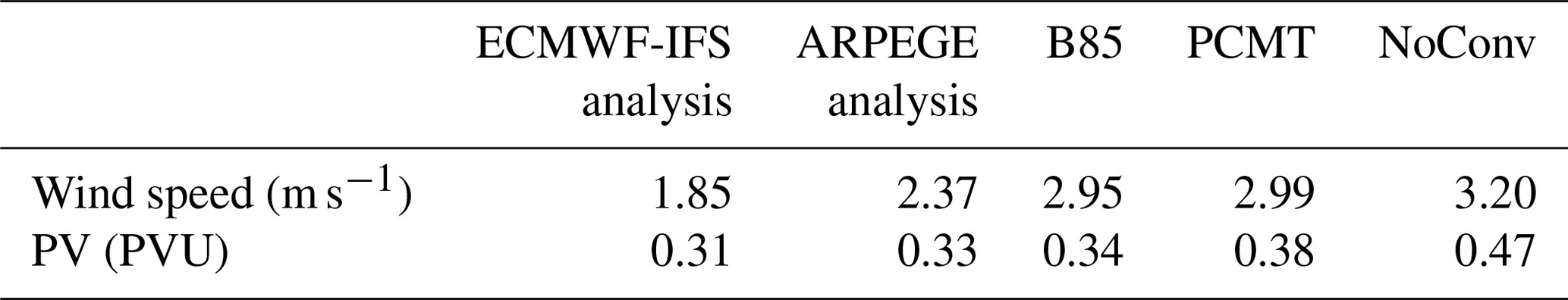
As the largest differences between the two forecasts appear in the middle of the troposphere, horizontal cross-sections of wind speed and PV are shown at 600 hPa in Fig. 3. In all simulations (references as well as forecasts), wind speed values higher than 40 m s−1, corresponding to the lower part of the jet stream, are located above and along the cold front of the Stalactite cyclone which is noticeable by a high gradient of potential temperature averaged between 750 and 850 hPa along an axis oriented from southeast to northwest.
Among the six datasets, PCMT and NoConv are the two simulations exhibiting the most intense jet stream with wind speed values beyond 40 m s−1 located east of a band of PV values exceeding 2 PVU along the cold front. The other datasets do not exhibit PV values as large as in PCMT and NoConv at 600 hPa in that region. More to the east, near the easternmost vertex of the triangular-shaped flight, a less well-defined secondary jet with values close to 30 m s−1 appears in ECMWF-IFS, ERA5, B85 and PCMT with different shapes and extensions. For instance, this secondary jet in B85 extends further to the northwest than in PCMT or in ECMWF-IFS and ERA5. This wind speed maximum around 600 hPa is somewhat reminiscent of the mid-level tropospheric jets described in Georgiev and Santurette (2009) and Kaplan et al. (2009). The ARPEGE analysis brings similarities with B85, which is not surprising as they both use the same model and the same deep convection scheme (B85). The ERA5 and ECMWF-IFS analyses are similar too as they both use the IFS model. This is confirmed by computing the root mean square (RMS) of the differences of each dataset with ERA5 (Table 1). Since the two analyses have a lower RMS difference with respect to ERA5 than the forecasts, it gives confidence in assessing the performance of the three forecasts as the three references are closer to each other than to the forecasts. Among the three forecasts, NoConv is the one leading to the highest RMS difference and in that sense it is less skilful than the other two. The PCMT and B85 have rather similar RMS values with those of PCMT being slightly higher. In terms of PV, it is clearly the band of high PV values to the west of the jet stream that increases the RMS error of PCMT with respect to ERA5, and more importantly that of NoConv. However, PCMT does not perform so differently from B85 because B85 has other significant differences with ERA5 along the third leg of the flight and related to the secondary jet that is extended too far northwestward as confirmed in Sect. 5.
The other PEARP members, differing only in their physical parameterisation of deep convection, turbulence, shallow convection and surface oceanic fluxes, as described in RW21, are also compared in an additional sensitivity study (Figs. S1 and S2 in the Supplement). Members 1, 2, 4, 5, and 9 predict a maximum of the jet stream near 300 hPa just as the B85 simulation (member 0) (Fig. S1). In contrast, members 3, 6 and 8 are marked by a jet stream maximum located lower, between 350 and 400 hPa and, in that sense, behave as in the PCMT simulation (member 7). Furthermore, the first group of members does not show any stratospheric air with a PV superior to 2 PVU in the mid-troposphere (600 hPa) whereas the second group shows systematic areas with PV higher than 2 PVU (Fig. S2). Notice that the common point of each group is the type of closure used in the deep convection schemes. Members 0, 1, 2, 4, 5 and 9 share the same deep convection scheme, namely B85 with a moisture convergence closure. In the other group, all members share a CAPE closure: members 6, 7 and 8 use the PCMT scheme and member 3 uses a modified version of B85 with a CAPE closure too. By analysing hindcasts of heavy precipitation events, Ponzano et al. (2020) also emphasised a clustering of the 10 PEARP members into 2 groups but their partition was dependent on the deep convection used (B85 vs. PCMT). In the present case as well as in RW21, the separation more clearly emerges according to the convection-parameterisation closure (moisture vs. CAPE).
To conclude, PCMT has a deeper jet stream than B85 over the cold front in association with higher positive PV values to the west and smaller negative PV values to the east in the mid-troposphere around 600 hPa. At this stage, it is rather difficult to determine which deep convection scheme is more realistic because the height and vertical structure of the jet in the three references (two analyses and ERA5) are usually in between the two runs. Since the two simulations with activated deep convection scheme behave in opposite ways and exhibit a large difference in the vertical structure of the jet stream, it is worth investigating the reasons of this difference as done in the next sections, in particular by analysing the properties of the WCB.
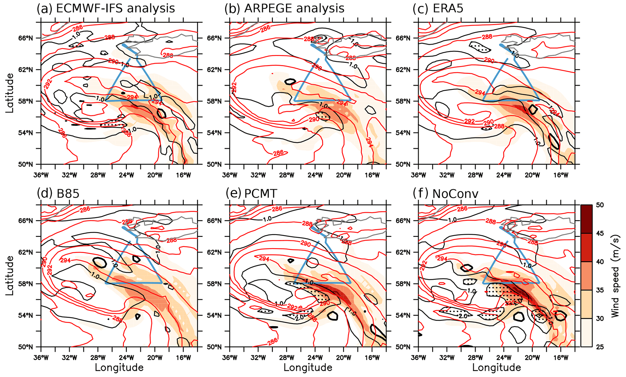
Figure 3Wind (shadings) and potential vorticity (black contours with hatched areas for values superior to 2 PVU and bold contours for 0 PVU) at 600 hPa with potential temperature averaged between 750 and 850 hPa (red contours) at 15:00 UTC, 2 October 2016 for (a) ECMWF-IFS analysis, (b) ARPEGE analysis, (c) ERA reanalysis, (d) simulation with B85, (e) simulation with PCMT and (f) simulation with explicit deep convection. The Flight F7 of the SAFIRE Falcon is shown as a blue line.
As the main difference in the jet stream highlighted in the previous section occurs during and near the SAFIRE flight on 2 October in the afternoon, the air streams crossing the flight are studied in the present section. They are represented by 48 h Lagrangian trajectories centred on the flight (see Sect. 2.4.2 for definitions). Trajectories satisfying the WCB criterion (300 hPa ascent in 24 h) are represented in Fig. 4a for B85 and Fig. 4b for PCMT. All WCB trajectories have a poleward direction along the cold front and then may turn cyclonically or anticyclonically as in the classical picture of the WCB (Schemm et al., 2013; Martinez-Alvarado et al., 2014).
The pressure along these trajectories, represented in colour, shows two ascending regions in the vicinity of the flight (e.g. near 25∘ W; 50∘ N and 40∘ W; 62.5∘ N). This confirms the flight clearly occurred in the main ascending region of the WCB.
Meridional section of the trajectories coloured by the heating rate are shown in Fig. 4c for B85 and Fig. 4d for PCMT. In both simulations the maximum heating undergone by the trajectories is about 2 K h−1 and logically occurs in the ascending part of the trajectories. Some cooling stage occurs in the lower troposphere before the trajectories reach the freezing point 0 ∘C (purple dots) due to evaporative or melting processes. In B85, strong cooling is obvious just below the freezing point between 45 and 50∘ N that is likely due to snow melting. Another slightly cooling area appears in both simulations: in the upper troposphere due to longwave radiation. Some large differences also exist between the two simulations. A large part of the PCMT trajectories present a strong heating of 2 K h−1 mainly coming from the large-scale heating (see Fig. S4) below the freezing level, while this phenomenon is much more reduced in B85, questioning the different behaviour between these two convection schemes in the liquid phase. This more intense heating occurring earlier along the trajectories and at lower altitude in PCMT has some implications in terms of PV tendencies as shown later.
Figure 4(a, b) Horizontal section of the pressure (shadings) along the warm conveyor belt trajectories crossing the Flight F7 for (a) B85 and (b) PCMT. (c, d) Meridional section of heating (shadings; 1st method of computation) along the warm conveyor belt trajectories crossing F7 for (c) B85 and (d) PCMT. Intersection with the iso-0 ∘C is represented by purple dots.
Figure 5a and b show the wind speed at 15:00 UTC on 2 October 2016 along the last half of the flight for B85 and PCMT, respectively, together with the difference in PV between PCMT and B85 (PCMT − B85) in each panel. Additionally, the positions of the WCB trajectories initialised along the legs of the flight are represented by the grey circles. Only the second and third legs of the Flight F7 are considered as very few trajectories satisfying the WCB criterion cross the first leg. Note that the abscissa is not the time but a trajectory index, which is the number of horizontal trajectory seeds along the flight.
Between 300 and 500 hPa, dipolar PV differences appear in the vicinity of the wind speed maxima with positive values to the east and anticyclonic to the west. It means that the PV gradient is stronger in B85 in the upper troposphere and is logically associated with stronger wind speed maxima at those levels. Between 500 and 700 hPa, opposite sign PV differences also appear on both sides of the jet, but here the positive values are to the west and negative ones to the east of the jet. It means there is a stronger PV gradient, which is associated with a stronger wind speed maxima in the mid troposphere and thus a deeper jet for PCMT. At the same levels but further away from the jet, the PV difference changes sign again (see trajectory index higher than 70). The opposite sign PV differences centred at trajectory index 70 reinforce the PV gradient in B85 with respect to PCMT and leads to the presence of a secondary jet at those levels for the former run, which has already been discussed when commenting Fig. 3d. Therefore, between 500 and 700 hPa, the PV difference exhibits a tripole in each leg, which is symptomatic for all sections crossing the cold front from 12∘ W–50∘ N to 28∘ W–62∘ N (Fig. 5c–d).
The positions of the WCB trajectories are located between 900 and 300 hPa for both simulations, but they are more numerous in the upper layer between 400 and 300 hPa in B85, particularly in leg 2 (compare Fig. 5a and b). The more numerous upper level WCB trajectories in B85 are in a positive PV difference, which means a lower PV in B85. As a strong heating occurs between 800 and 400 hPa followed by a rapid decrease above the 400 hPa level (see Fig. 4c and d), it indicates that the vertical gradient of the heating is negative at 400 hPa and above. Hence, the WCB trajectories at the time of the flight undergo a negative PV tendency above 400 hPa and the more numerous WCB trajectories in B85 at those levels induce more PV destruction than those in PCMT. It provides an explanation for the smaller PV east of the jet, stronger PV gradient, and stronger wind speed in B85 at pressure lower than 400 hPa. Between 500 and 700 hPa along the cold front, most of the WCB trajectories initialised in the warm sector are located in the negative PV difference (Fig. 5c, d). Very few of them, initialised along the flight, are within the positive PV difference to the east of the main jet (see trajectory index between 45 and 60 in Fig. 5a–b).
To better explain the deeper jet stream in PCMT, the next section focuses on the jet between 500 and 700 hPa, where differences between PCMT and B85 are the highest. Particularly, the origins of the positive PV difference (black dots in Fig. 5a–b) and negative PV difference (green dots) located on the warm side of the jet stream are studied. The reasoning is the following: wind differences observed in Figs. 2 and 3 at 600 hPa are related to PV gradient differences, which themselves can be explained by following backward Lagrangian trajectories initialised in the area with the highest PV differences. Computation of these trajectories allows identification of the time when the PV values of the two runs diverge and the underlying processes.
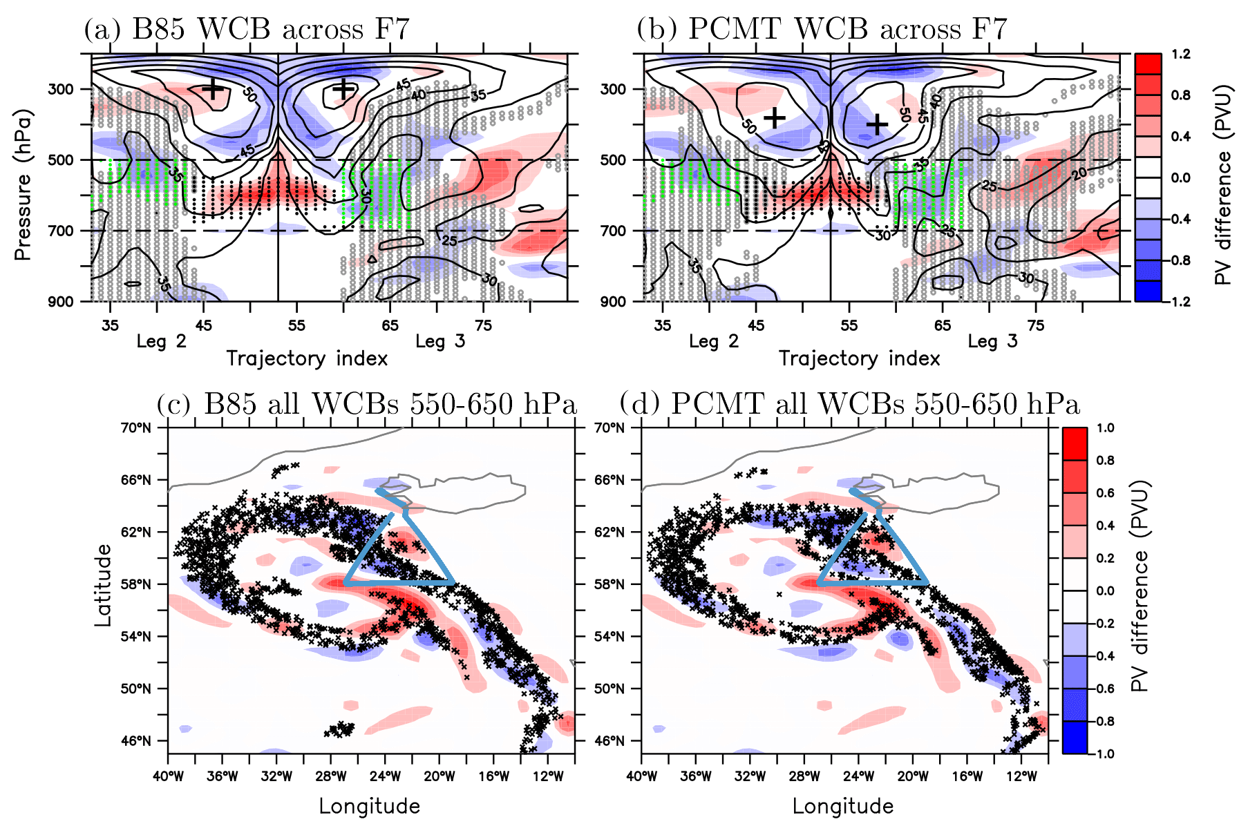
Figure 5(a, b) Vertical cross-section of the difference (PCMT − B85) in PV (shading) along the second and third leg of Flight F7 at 15:00 UTC, 2 October 2016. The wind speed (black contours) and intersection of WCB trajectories with an ascent of 300 hPa in 24 h with F7 (grey circles) are shown for (a) B85 and (b) PCMT. In panels (a) and (b), the thick crosses represent the wind speed maxima in legs 2 and 3 for B85 and PCMT, respectively. Trajectories where PV differences are positive and negative between 500 and 700 hPa are in black and green dots, respectively. (c, d) PV difference at 600 hPa (shading) and WCB trajectories, initialised in the warm sector, positions between 550–650 hPa (crosses) at 15:00 UTC 2 October 2016 for (c) B85 and (d) PCMT. The flight is shown by the blue line.
4.1 Positive PV difference on the cold air side of the jet
To investigate the origin of the positive PV difference, the 24 h backward trajectories, whose seeding point is represented by black dots on Fig. 5a and b, are considered. Figure 6a shows the time evolution of PV averaged over all trajectories reaching the positive PV difference along legs 2 and 3 (red and orange, respectively for B85; blue and cyan, respectively for PCMT). The first striking result is that the averaged PV is almost the same at the initial time (16:00 UTC on 1 October) between the two simulations while they differ by about 0.3 PVU at the final time (16:00 UTC on 2 October). It clearly shows that the higher PV in PCMT than B85 at the time of the flight (15:00 and 15:45 UTC on 2 October for leg 2 and 3, respectively) is solely due to diabatic PV modification along trajectories. More precisely, between 00:00 and 04:00 UTC on 2 October the B85 and PCMT curves move away from each other (compare the red and blue curves or the orange and cyan curves). After 04:00 UTC, the PV difference between B85 and PCMT is maintained whatever the leg, even though the separation distance between the curves may be temporarily reduced.
The time evolution of the PV tendencies computed by summing the tendencies due to heating and friction is shown in Fig. 6b for leg2 (bold solid lines). The good correspondence between the sign of that sum (Fig. 6b) and the slope of the PV evolution (Fig. 6a) shows that the budget is correctly done. For B85, between 16:00 and 22:00 UTC, PV increases and the sum of all terms is positive, while after 22:00 UTC, PV tends to slightly decrease consistent with near zero or negative PV tendency. Only at later times, after 12:00 UTC on 2 October, PV increases slightly. For PCMT, the tendency is first near zero and the PV does not change much prior to 20:00 UTC on 1 October but after that short period, the PV tendency is most of the time positive and higher than that of B85 except near 03:00 UTC on 2 October or 10:00 UTC on 2 October.
The PV tendencies decomposition into heating (thin line) and friction (thin dashed line) parts clearly shows that the PV fluctuations are dominated by the heating. In particular, positive PV tendencies are solely due to the heating. Figure 6c and d represent the vertical profiles of PV tendencies and heating averaged over all grid points where there is a trajectory from leg 2 for B85 and PCMT, respectively. One large difference between the two figures concerns the pressure distribution along the trajectories (red or blue dashed curves). For B85, they are clustered in a single group always transported in the middle of the troposphere during 24 h before reaching the positive difference of leg 2 (see dashed red curves in Fig. 6c). Depending on how they are positioned relative to the heating or cooling regions, they may undergo PV increase or decrease. Indeed, as the PV tendency is proportional to the vertical heating gradient (see e.g. Fig. 4 of Wernli and Davies, 1997), the PV tendency is positive under the heating and negative above. For instance, the slight PV increase between 16:00 and 22:00 UTC on 1 October or after 12:00 UTC on 2 October is explained by the fact that the trajectories are above a cooling region. In contrast, for PCMT, the trajectories are clustered into two well-separated groups, one half transported in the middle of the troposphere as in B85 but the other half starting in the boundary layer and suddenly rising at 04:00 UTC 2 October (see dashed blue curves in Fig. 6d). Slightly before and during the beginning of the ascents of the latter trajectories (i.e. from 00:00 to 04:00 UTC on 2 October), PV rapidly increases because the trajectories are below a region of strong heating. It is precisely during this period that the two averaged PV in B85 and PCMT diverge from each other (Fig. 6a) and the PV tendencies are largely different (Fig. 6b). When the same trajectories go above the heating, they undergo a short period of PV decrease between 08:00 and 10:00 UTC but they rapidly go above a cooling region after 12:00 UTC when they catch up the first group of trajectories and their PV increases once again.
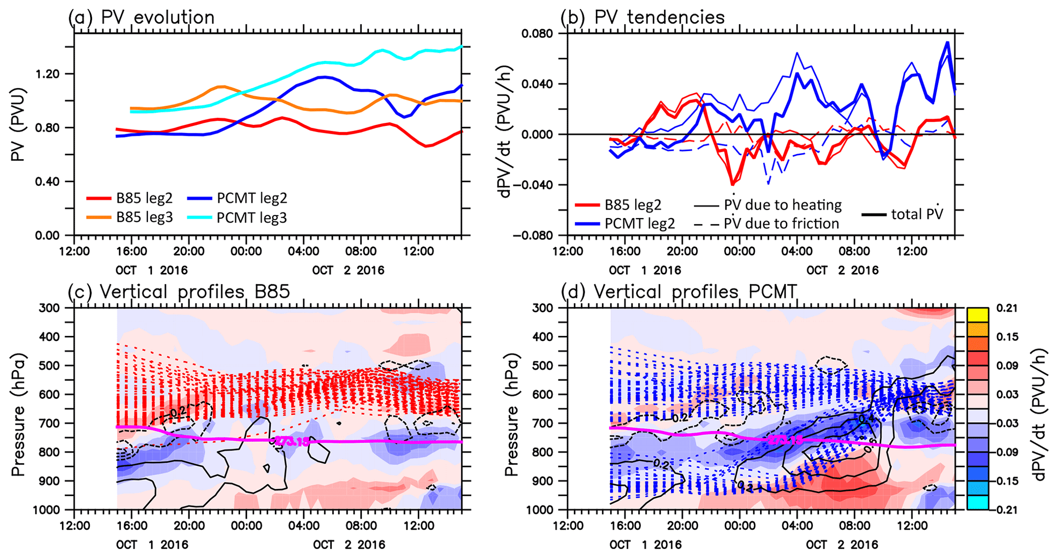
Figure 6(a) Time evolution of PV for trajectories reaching the positive PV difference in leg 2 (red line for B85 and blue line for PCMT) and leg 3 (orange line for B85 and cyan line for PCMT). (b) Time evolution of PV tendencies due to heating (thin solid lines), friction (thin dashed lines) and total (bold solid lines) for B85 (red) and PCMT (blue). Vertical profiles, according to time, of heating (dashed and solid contours for negative and positive values, respectively; second method of computation) and PV tendency due to heating (shading) along trajectories reaching the positive PV difference for (c) B85 (dashed red curves) and (d) PCMT (dashed blue curves), respectively. The iso-0 ∘C is the purple line.
Figure 7 helps to further visualise the position of the trajectories with respect to the heating when PV values of each simulation are sufficiently different from each other (Fig. 6a). For this purpose, the chosen time is 03:00 UTC on 2 October. As previously observed in Fig. 6c, trajectories from the positive difference do not present any ascent in B85 (Fig. 7a). They are all transported west of the heating area behind the cold front around 650 hPa and the iso-304 K (Fig. 7a, c). In PCMT, the group of trajectories around 650 hPa have more or less the same position relative to the main heating area as the one in B85 (Fig. 7b, d). However they are above a well-marked cooling region near 24–26∘ W and 700 hPa and undergo a slightly larger PV increase than those for B85. The heating budgets in Figs. S3 and S4 for B85 and PCMT, respectively, show that the cooling region is due to both radiation and turbulence at the top of mid-level convective clouds in the cold sector of the cyclone. This increase in PV for trajectories moving in the mid-troposphere over the cold sector can be seen at different time intervals in both runs (between 15:00 UTC on 1 October and 00:00 UTC on 2 October or after 12:00 UTC on 2 October in Fig. 6c, d) but the PV increase appears to be more important on average in PCMT (compare the reddish colours between 700 and 600 hPa in Fig. 6c and d). The other group of trajectories found in PCMT is located at 22∘ W and 900 hPa. They are located in the lowest and most western part of the main heating area ahead of the cold front, which is dominated by large-scale cloud heating (Fig. S4), and will rapidly ascend during the following hours (Fig. 6d).
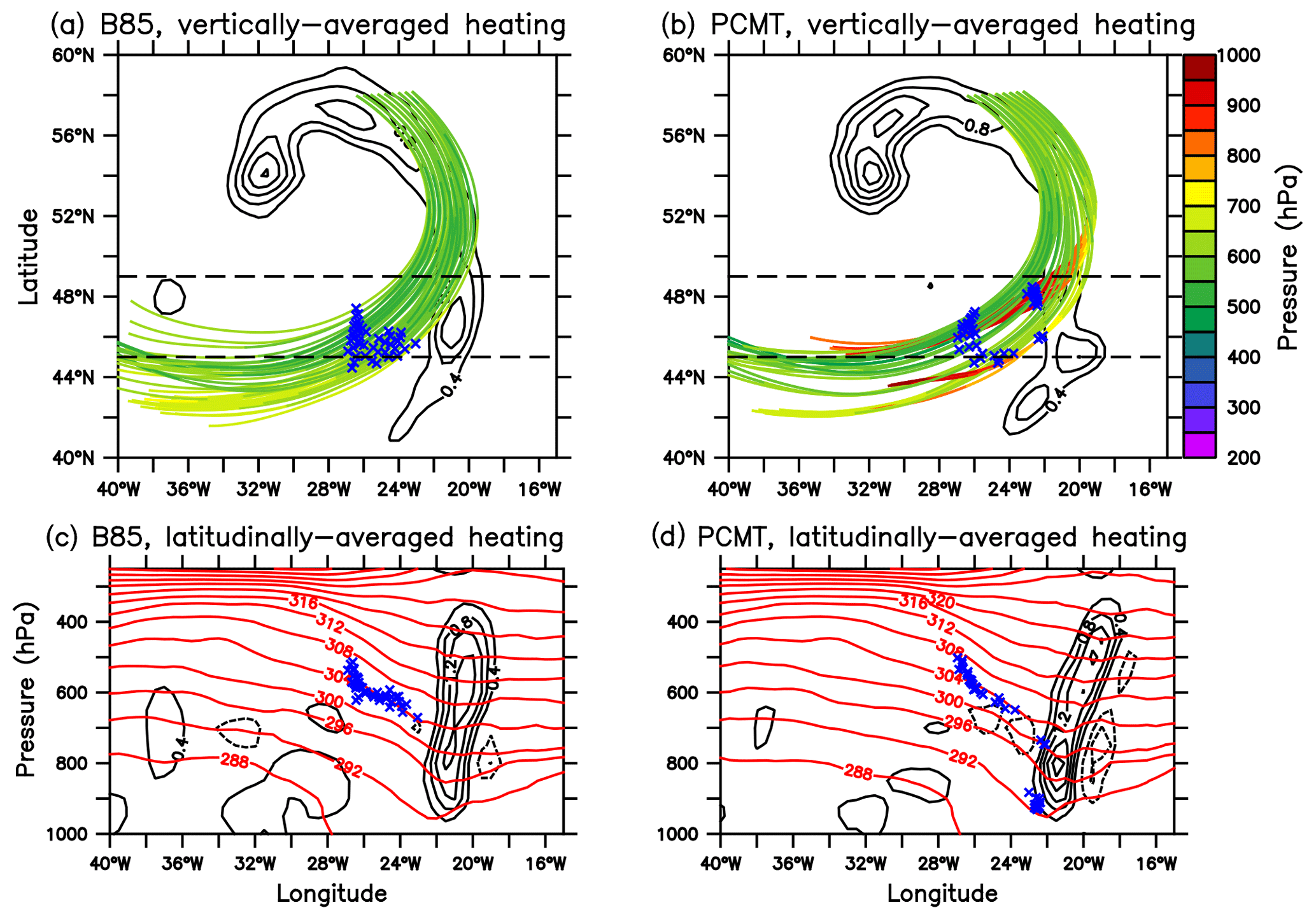
Figure 7Pressure (shading) along trajectories reaching the positive PV difference in leg 2 for (a) B85 and (b) PCMT, vertically averaged heating between 300 and 900 hPa (black contours; units: 0.4 K h−1) and trajectories position (blue crosses) at 03:00 UTC, 2 October. Vertical cross-sections of heating averaged between 45∘ and 49∘ N (black contours; second method of computation), potential temperature (red contours) and trajectory positions (blue crosses) at 03:00 UTC 2 October for (c) B85 and (d) PCMT.
To conclude, the higher PV obtained in PCMT than B85 on the cold air side of the jet stream is mainly due to diabatic processes occurring between 00:00 and 04:00 UTC 2 October during which half of the PCMT trajectories rapidly ascend and undergo a PV increase below a strong heating area. This heating is mainly due to large-scale latent heating and, to a lesser extent, due to convection heating (Figs. S3, S4). Some of these trajectories exceeding a 300 hPa ascent in 24 h satisfy the WCB criterion and are thus identified with grey circles in Fig. 5b near trajectory indexes 45–50. The presence of such ascending trajectories very near the core of the cold front is unexpected and is associated with a more important overlapping of the heating area and the horizontal temperature gradient in PCMT than in B85 (not shown). An additional factor to explain the difference in PV between the two runs concerns the group of trajectories evolving in the middle of the troposphere: in PCMT, they are more often subject to PV increase in the presence of cooling areas below them at the top of convective mid-level clouds in the cold sector of the cyclone. In B85, this happens less regularly along similar trajectories.
4.2 Negative PV difference on the warm air side of the jet
The same approach based on backward trajectory (seeded at the green dots in Fig. 5a, b) is adopted to better understand the origin of the negative PV difference to the east of the jet, which is mainly embedded in the WCB region. At the time of the flight (15:00 UTC on 2 October), the averaged PV is about 0.3 PVU lower in PCMT than in B85 whatever the leg (Fig. 8a). For leg 3, the difference in PV rapidly increases from 04:00 to 08:00 UTC on 2 October while for leg 2, it increases from 12:00 to 15:00 UTC on 2 October. Even though the timing is different, for both legs the PV difference is small at the initial time (16:00 UTC on 1 October) and the PV difference has a diabatic origin occurring during the last 12 h before reaching the flight legs.
Let us now focus on the negative PV difference of leg 2. For both PCMT and B85, PV first increases and then decreases. However, the PV variations are larger in PCMT than B85. This difference is due to a higher PV tendency in PCMT which results from the higher heating term in the PV tendency budget. The friction contribution only partly offsets the differences due to the heating terms during the PV increase phase (Fig. 8b). The heating being stronger in PCMT than B85 (maxima are about 2 K h−1 for PCMT and 1.4 K h−1 for B85), its gradient is stronger leading to higher amplitude PV tendency in the former case (Fig. 8c–d). The heating is also more vertically stacked in the lower troposphere in PCMT in such a way that the trajectories are already all advected in a region above the heating maximum in PCMT after 10:00 UTC on 2 October and undergo a negative PV tendency (Fig. 8b, d). During this later period, the B85 trajectories are advected near a region of maximum heating and have thus near zero PV tendency (Fig. 8b, c).
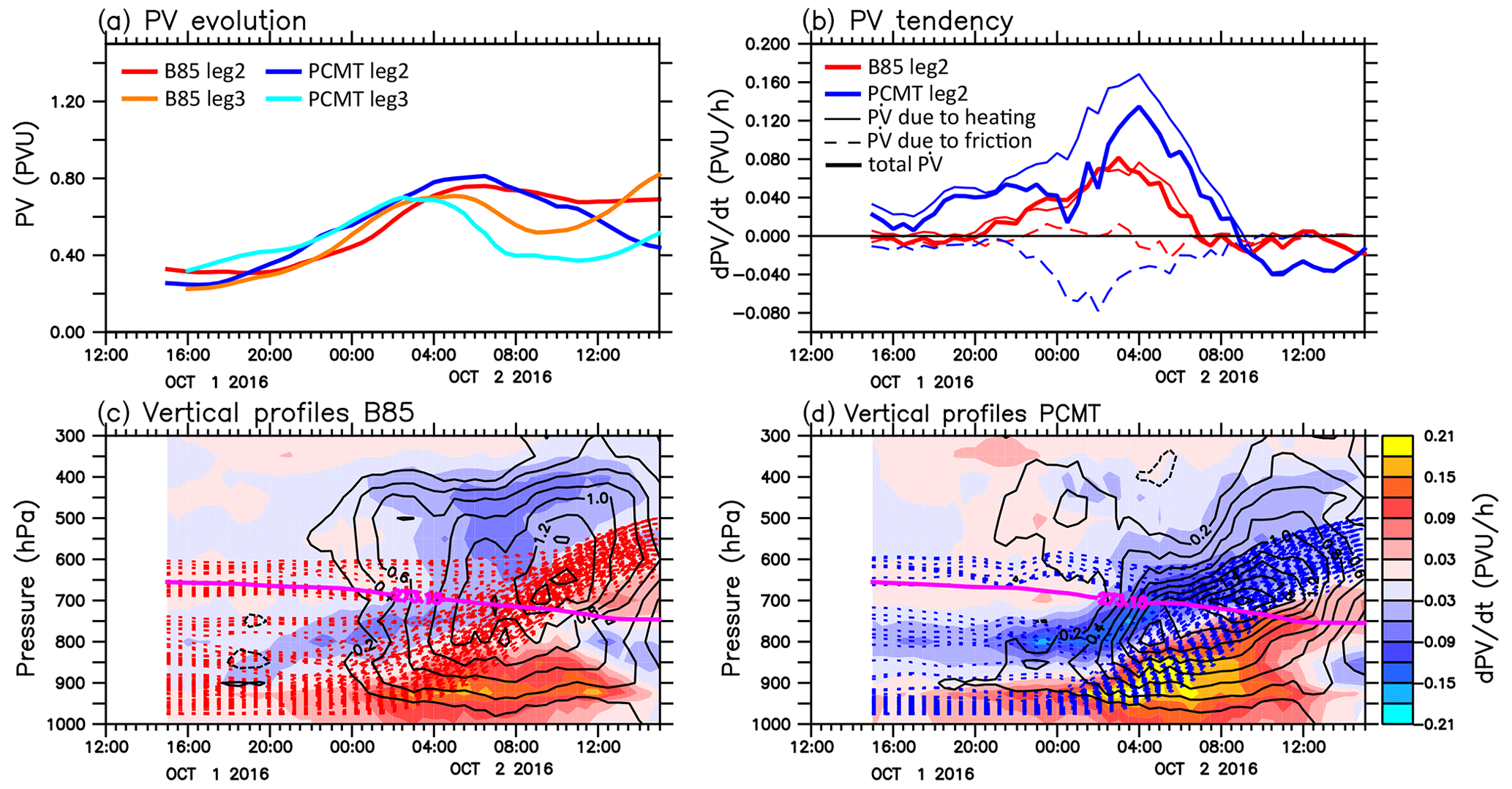
Figure 9 provides horizontal and zonal sections of the position of the trajectories with respect to the heating at 12:00 UTC on 2 October, i.e. the time when the PV difference between PCMT and B85 starts to increase. At the initial time, the majority of trajectories were located in the boundary layer of the warm sector of the cyclone whatever the simulation (Fig. 9a–b). At the time of the figure, all trajectories lie within the strong heating region ahead of the cold front. However, their positions relative to the vertical heating gradient largely differ between PCMT and B85. This is mainly due to two distinct features in the heating fields. The B85 heating extends more to the upper troposphere and is more vertical whereas PCMT heating is more confined in the middle troposphere and is marked by an eastward tilt with height. The latter tilt is rather systematic whatever the time chosen (see Figs. 7d and 9d). These two distinct features place the trajectories in a region of negative heating gradient and thus negative PV tendency in PCMT while the heating gradient is weak for the B85 trajectories. Thus, contrary to B85, the PCMT trajectories are already passing over the main heating area ahead of the cold front and already lose PV before reaching the flight leg.
In summary, the deeper jet stream in PCMT than B85 can be explained by distinct diabatic processes occurring on both sides of the jet in the middle troposphere. On the cold air side, half of the PCMT trajectories undergo some PV increase as they travel below the heating before reaching the middle troposphere while all B85 trajectories keep travelling in the middle troposphere. On the warm air side, PCMT trajectories undergo a more rapid PV decrease because they already pass over the heating, which is more confined at lower levels and appears earlier than in B85. Such difference in vertical heating has already been observed in Fig. 4 and is partly linked to a different behaviour of deep convection schemes in the liquid phase. This leads to a negative PV difference in mid-troposphere in PCMT while this anomaly appears more in the upper level in B85. This induces a PV difference between PCMT and B85 that reinforces the PV gradient at mid-levels and thus the jet in PCMT relative to B85.

As it is the difference in the heating structure that makes the difference in the vertical structure of the jet stream, and as the heating is linked to cloud formation and microphysics, a comparison is made between the ice water content (IWC) of the model simulations and the one retrieved from the RALI observations in Fig. 10.
Only the second half of the flight is considered. To better compare to ARPEGE simulations, observations are interpolated at the model outputs resolution (0.5∘ grid spacing roughly corresponding to 180 s at the aircraft speed) in Fig. 10. Two IWC products are retrieved from the observations using the Varcloud algorithm (Delanoë and Hogan, 2008; Cazenave et al., 2019): one is based on the radar RASTA measurements only (Fig. 10a) using both reflectivity and Doppler velocity, and the other on RALI measurements, i.e. assimilating radar reflectivity and lidar backscatter (Fig. 10b). Since the lidar is more sensitive to small particle and small hydrometeor contents, the RALI retrieval usually leads to smaller IWC than the RASTA retrieval as confirmed by comparing Fig. 10a and b. Note that these two retrievals do not use the same microphysical assumptions due to the difference in sensitivity and penetration capability of these two instruments. As described in Cazenave et al. (2019), the main uncertainties in the retrieval come from the mass : size and area : size relationships. Therefore, the comparison between these two retrievals gives an idea of the uncertainties related to those retrievals.
As the flight crosses the WCB region twice, two zones with high IWC are observed in each retrieval: one between 14.5 and 15 h and the second between 15.4 and 16 h. The peak values of the retrieved IWC are near 2000 mg m−3 (Fig. 10a, b) whereas those of the model simulations do not exceed 400 mg m−3 (Fig. 10c, d). The IWC values of the model simulations strongly depend on the snow falling speed which is a constant prescribed in the model. In the present simulations, its value is 1.5 m s−1. Additional sensitivity experiments made by setting its value to 0.6 m s−1 led to IWC peak values near 800 mg m−3 (not shown). So even in the case of low snow falling velocity, the IWC is largely underestimated in the model. In a supplementary figure (Fig. S5), the IWC divided by the cloud fraction, which could be thought as being more relevant to compare to observations, also fails to reproduce the high IWC values detected in the observations. This result is not surprising following Mazoyer et al. (2022) who found similar underestimation in regional model simulations of the Stalactite cyclone. The comparison between the two simulations shows that the peak values are slightly higher in B85 than in PCMT but the difference is too weak to be conclusive.
The difference in IWC spatial distribution is worth commenting on, especially with respect to the previous sections. The flight crossed the separating area between the cloudy WCB region with high IWC values and the clear sky region close to the cyclone center twice, at 14.9 and 15.5 h. These two transitions are easily visible at 15.0 and 15.5 h in B85 but are much less clear in PCMT. In the latter run, in the observed clear-sky region, there are clouds (Fig. 10d) whose tops are at about 500 hPa. Also many trajectories belonging to that area between 15.0 and 15.5 h satisfy the WCB criterion (see grey circles in Fig. 10c) and correspond to the trajectories which undergo strong heating during their ascent between 900 and 600 hPa (Fig. 6d). Figure S6 shows the same patterns but with model outputs and interpolation made over a 0.1∘ × 0.1∘ grid. The results are qualitatively the same but the scales of the clouds are more representative of the model resolution.
To conclude, even though both simulations fail to produce the high values of IWC seen in the observations, the spatial distribution of IWC differs between the two simulations. B85 better represents the abrupt transition between the cloudy region of the WCB and the clear sky region behind the cold front.
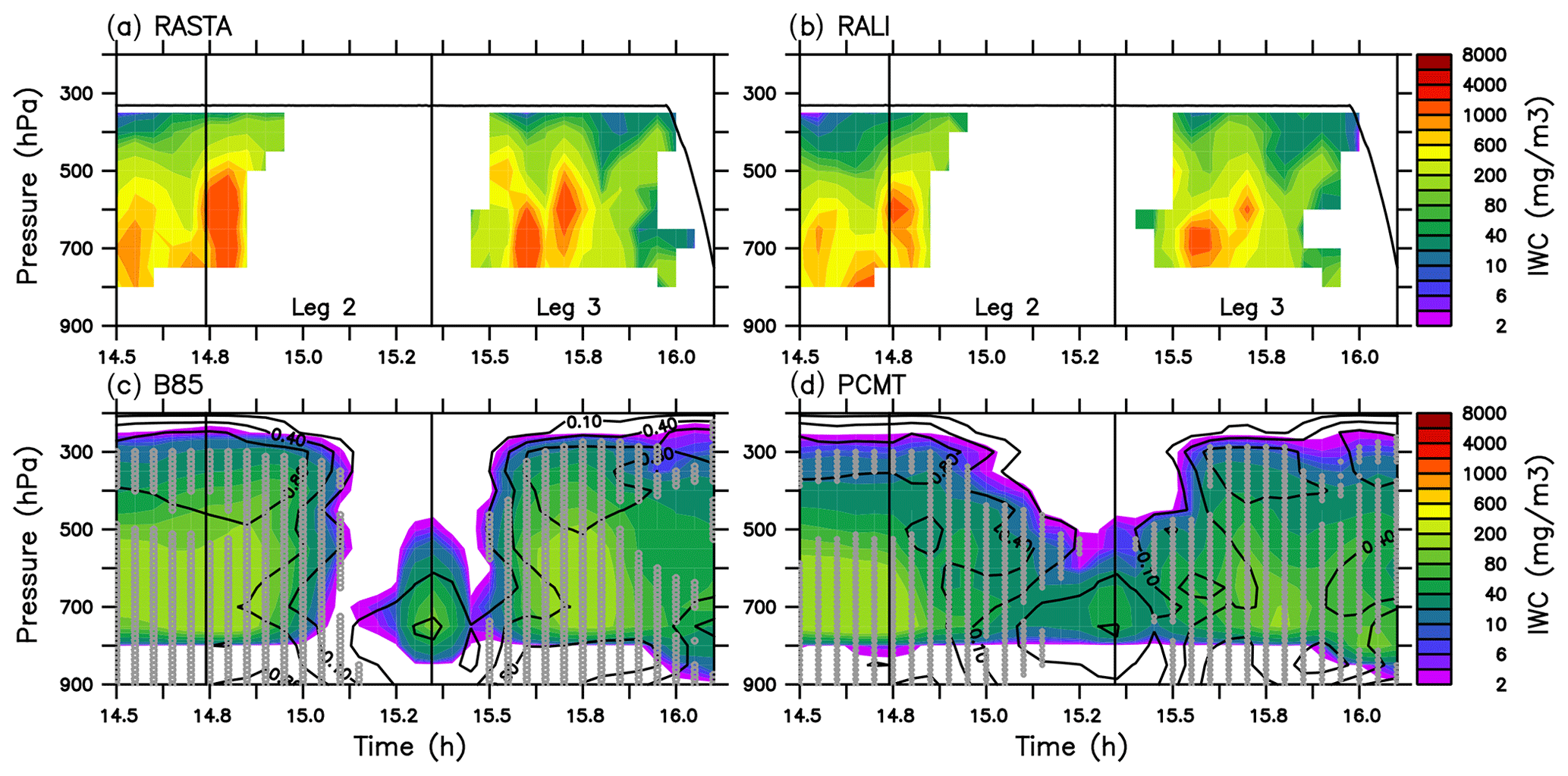
Figure 10Ice water content (mg m−3) for (a) retrieval from radar RASTA (b) retrieval from radar-lidar RALI along legs 2 and 3 of F7 (airborne level in black line). Total ice water content (snow+cloud ice water; mg m−3; shading) and cloud fraction (black contours) for (c) B85 and (d) PCMT respectively. Grey circles represent WCB trajectories crossing F7.
To determine which run better represents the jet stream, the wind speed of the simulations is compared with those measured by the radar RASTA and on board the aircraft in Fig. 11. There is generally a good correspondence between the wind speed measured by the aircraft and that measured by the radar (Fig. 11a). However, as there are no clouds from 14.9 and 15.5 h, no wind speed observations from the radar are available. Hence, the jet stream, which is crossed twice at 15.1 and 15.5 h, is only very partially covered by the radar measurements (compare the colour shadings with the contours). The radar measurements are useless to look precisely at the vertical structure of the jet stream and the aircraft measurements provide information at a given level only. At the aircraft level, the two runs give similar differences with some underestimation of winds between 15.6 and 16.0 h. There is only one region where the two simulations behave very differently: this is between 15.6 and 16 h and near the 500–700 hPa layer (Fig. 11b–c). While there is a minimum in wind speed in the observations as well as in PCMT in that region, a secondary jet is present in B85 with values near 30 m s−1, which was already discussed in Sect. 3. The wind speed in B85 is overestimated by about 6–9 m s−1. According to Fig. 5a, this wind speed anomaly is linked to the stronger PV gradient in B85 than PCMT associated with the dipolar PV difference located at 600 hPa at the end of the flight (trajectory index from 65 to 75). Comparison with radar measurements leads to the same conclusion as the comparison made with (re)analyses in Sect. 3. The secondary jet in B85 along leg 3 is not present in any of these references.
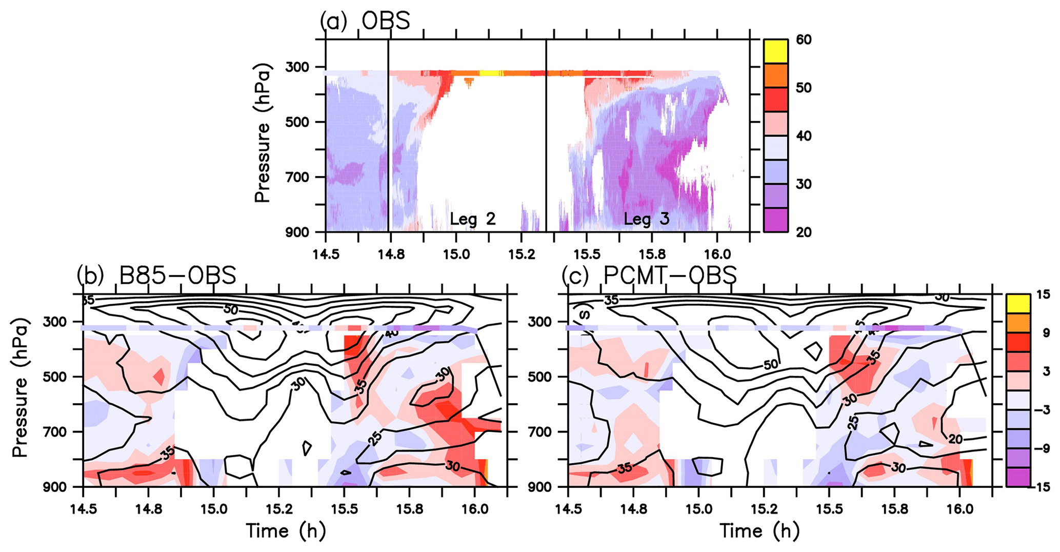
Figure 11(a) Wind speed observations from RASTA and aircraft at full resolution. Wind speed anomaly with respect to observations interpolated at model resolution (shading) and wind speed (black contour) for B85 (b difference B85-Obs.) and PCMT (c difference PCMT-Obs.).
The present study and our companion paper (Rivière et al., 2021, RW21) provide a general view of the impact of deep convection representation in a global numerical weather model on the WCB of an explosive extratropical cyclone observed during NAWDEX and on the jet stream aloft. Three simulations of the Météo-France global model ARPEGE, which only differ by their deep convection representation, are investigated. Two of them use the model with a distinct deep convection scheme activated: one with the scheme developed in Bougeault (1985, B85), the other one with the one from Piriou et al. (2007, PCMT). In the last ARPEGE simulation, called NoConv, no deep convection scheme is activated. The companion paper investigated the general behaviour of WCB activity in the three simulations and its impact on the jet stream in the WCB outflow region above the bent back warm front. The present study was dedicated to the impact of these parameterisation schemes on the jet stream in the WCB ascending region above the cold front.

Figure 12Schematic representing differences between the two convection schemes in latent heating and PV tendencies.
The systematic comparison made between the three simulations led to the following conclusions:
-
The deep convection representation has an important effect on the vertical structure of the jet stream above the cold front: the jet stream is deeper in NoConv simulation, i.e. without parameterised deep convection, and in PCMT simulation than in B85 simulation.
-
The deeper jet stream in NoConv and PCMT compared to B85 is associated with a deepening of the dynamical tropopause (i.e. higher PV) behind the cold front and with more PV destruction ahead of the cold front in middle troposphere (600 hPa). The difference in PV between PCMT and B85 is marked by a dipolar PV difference centred on the jet core which reinforces the PV gradient and thus the jet in middle troposphere. This dipolar PV difference is due to differences in diabatic processes between the two simulations.
-
The same tropopause deepening is observed for PEARP members sharing the same deep convection closure, suggesting, as in RW21, the key role played by that closure on the jet stream structure.
-
On the cold air side of the jet, the high PV area of the dipolar difference is due to different behaviours of the Lagrangian trajectories reaching that area. In B85, they form an homogeneous group of trajectories staying at the same pressure level in middle troposphere and undergoing modest PV fluctuations in the cold sector. In contrast, the PCMT trajectories are clearly separated into two groups. One group of trajectories behaves like in B85 with weak pressure variations but is more subject to PV increase because the trajectories pass over a more marked cooling due to radiation and turbulence above cold sector convective clouds. The second group behaves in a totally different manner; they come from the boundary layer, ascend on the western flank of the region of strong latent heating and undergo PV increase, before joining the first group at the same altitude. The strong latent heating is mainly due to large-scale cloud and to a lesser extent to convection. The trajectories of the second group satisfy the WCB criterion of 300 hPa ascent in 24 h chosen in the present study.
-
On the warm air side of the jet, WCB Lagrangian trajectories are quite similar but their behaviour, synthesised in Fig. 12, is clearly different between the two deep convection schemes. With PCMT, WCB trajectories pass earlier through the main heating area as it is located at lower altitude than in B85 (Fig. 12a). Hence, an earlier decrease of PV occurs for the trajectories in PCMT and negative PV tendency appears in the middle troposphere (Fig. 12b). This is to be contrasted with B85 where the peak values of the heating extend further upward and much less PV destruction occurs at mid-tropospheric levels. This difference in the altitude of the heating maximum explains the difference in PV ahead of the cold front in middle troposphere.
Then, the question of the realism of the different hindcasts has been addressed by comparing them to different (re)analysis datasets and to NAWDEX airborne observations. It led to the following conclusions:
-
The jet stream structure in (re)analysis datasets as provided by ERA5 and ECMWF/Météo-France operational analyses lies in between the B85 simulation on the one hand and the PCMT and NoConv simulations on the other hand. For instance, the altitude of the jet stream maximum in B85 is located above those in (re)analysis datasets, which themselves are above those in PCMT and NoConv. Another example concerns the peak values of PV near 600 hPa: in descending order there are the PCMT and NoConv values followed by (re)analysis datasets and finally B85 values.
-
The ice water content retrieved from the radar-lidar measurements using the Varcloud algorithm (Delanoë and Hogan, 2008; Cazenave et al., 2019) shows a clear separation between the cloudy region ahead of the cold front and the ice-cloud free region behind it. This separation is well identified in B85 but not in PCMT. Behind the cold front, B85 is more realistic than PCMT which exhibits too many mid-level clouds.
-
As the main jet is largely embedded in clear sky regions, the Doppler cloud radar observations are useless to determine which run is more realistic. However, analysis of the wind speed anomalies with respect to the observations in cloudy regions ahead of the cold front indicate that B85 creates a secondary jet in the mid-troposphere which does not appear in the observations nor in PCMT. Therefore, in that particular region, the PCMT simulation performs better and this is due to the earlier PV destruction in PCMT.
Therefore, the present analysis cannot state which hindcasts better represent the observations as the conclusion is strongly dependent on the regions we are looking at. However, it shows that PCMT and B85 have drastically different behaviours with the former being close to the simulation without parameterised convection. The overall picture provided by the present study and the companion paper is the following: in the B85 simulation the heating is more homogeneously distributed ahead of the cold front and along the bent back warm front, it extends further up leading to stronger PV destruction in the upper troposphere that accelerates the ridge building in the WCB outflow region. In PCMT and NoConv simulations the heating is more heterogeneous, especially in NoConv, it extends less in the upper troposphere and the loss of PV happens at a lower altitude ahead of the cold front and makes the jet deeper in that region. Finally, note that such a difference between the two deep convection schemes is systematic as it was also found for other lead times and initial conditions but also above the cold front of the following extratropical cyclone on 4–5 October 2016 (NAWDEX IOP7; not shown).
The important question that follows is: where do these different behaviours come from? A first answer found in this study is the different deep convection parameterisation closure used, namely the CAPE for PCMT and moisture convergence closure for B85. However, further sensitivity studies will be planned in order to better identify effects of different parts of the deep convection schemes on mid-latitude cyclogenesis and the jet stream.
Data are available by contacting the corresponding author. ERA5 data are accessible via the climate data store (https://cds.climate.copernicus.eu, last access: April 2021; DOI: https://doi.org/10.24381/cds.bd0915c6, Hersbach et al., 2018b).
Worldview NASA picture is available at https://go.nasa.gov/3xOhRhv (last access: May 2022, Schmaltz et al., 2021).
The supplement related to this article is available online at: https://doi.org/10.5194/wcd-3-863-2022-supplement.
GR and PA designed the initial study. MW and GR performed the data analysis and made the figures. MW computed the Lagrangian trajectories. CL performed the ARPEGE simulations with the help of JMP. PA developed the Lagrangian trajectory algorithm. JD, QC, and JP provided the observational datasets. All authors contributed to the scientific discussions and to the paper writing
The contact author has declared that neither they nor their co-authors have any competing interests.
Publisher's note: Copernicus Publications remains neutral with regard to jurisdictional claims in published maps and institutional affiliations.
The study benefited from discussions with the participants of the DIP-NAWDEX (DIabatic Processes in the North Atlantic Waveguide and Downstream impact EXperiment) project which is supported and funded by the Agence Nationale de la Recherche (ANR). It also benefited from discussions with our international NAWDEX partners during annual workshops. ERA5 datasets have been generated under the framework of the Copernicus Climate Change Service (C3S). We thank Heini Wernli for downloading the ECMWF-IFS operational analysis data and Hanin Binder for sending them to us. We acknowledge the use of imagery from the NASA Worldview application (https://worldview.earthdata.nasa.gov, last access: May 2022), part of the NASA Earth Observing System Data and Information System (EOSDIS).
This research has been supported by the Agence Nationale de la Recherche (grant no. ANR-17-CE01-0010-01). The airborne measurements and the SAFIRE Falcon flights received direct funding from IPSL, Météo-France, INSU-LEFE, EUFAR-NEAREX, and ESA (EPATAN, contract no. 4000119015/16/NL/CT/gp).
This paper was edited by Lukas Papritz and reviewed by two anonymous referees.
Attinger, R., Spreitzer, E., Boettcher, M., Wernli, H., and Joos, H.: Systematic assessment of the diabatic processes that modify low-level potential vorticity in extratropical cyclones, Weather Clim. Dynam., 2, 1073–1091, https://doi.org/10.5194/wcd-2-1073-2021, 2021. a
Baumgart, M., Riemer, M., Wirth, V., and Teubler, F.: Potential Vorticity Dynamics of Forecast Errors: A Quantitative Case Study, Mon. Weather Rev., 146, 1405–1425, https://doi.org/10.1175/MWR-D-17-0196.1, 2018. a
Binder, H., Rivière, G., Arbogast, P., Maynard, K., Bosser, P., Joly, B., and Labadie, C.: Dynamics of forecast-error growth along cut-off Sanchez and its consequence for the prediction of a high-impact weather event over southern France, Q. J. Roy. Meteor. Soc., 147, 3263–3285, https://doi.org/10.1002/qj.4127, 2021. a
Blanchard, N., Pantillon, F., Chaboureau, J.-P., and Delanoë, J.: Organization of convective ascents in a warm conveyor belt, Weather Clim. Dynam., 1, 617–634, https://doi.org/10.5194/wcd-1-617-2020, 2020. a
Blanchard, N., Pantillon, F., Chaboureau, J.-P., and Delanoë, J.: Mid-level convection in a warm conveyor belt accelerates the jet stream, Weather Clim. Dynam., 2, 37–53, https://doi.org/10.5194/wcd-2-37-2021, 2021. a, b
Bougeault, P.: A simple parameterization of the large-scale effects of cumulus convection., Mon. Weather Rev., 113, 2105–2121, 1985. a, b, c, d
Bruneau, D., Pelon, J., Blouzon, F., Spatazza, J., Genau, P., Buchholtz, G., Amarouche, N., Abchiche, A., and Aouji, O.: 355-nm high spectral resolution airborne lidar LNG: system description and first results, Appl. Optics, 54, 8776–8785, https://doi.org/10.1364/AO.54.008776, 2015. a
Cazenave, Q., Ceccaldi, M., Delanoë, J., Pelon, J., Groß, S., and Heymsfield, A.: Evolution of DARDAR-CLOUD ice cloud retrievals: new parameters and impacts on the retrieved microphysical properties, Atmos. Meas. Tech., 12, 2819–2835, https://doi.org/10.5194/amt-12-2819-2019, 2019. a, b, c
Chagnon, J. and Gray, S. L.: Horizontal potential vorticity dipoles on the convective storm scale, Q. J. Roy. Meteor. Soc., 135, 1392–1408, 2009. a
Chagnon, J., Gray, S. L., and Methven, J.: Diabatic processes modifying potential vorticity in a North Atlantic Cyclone, Q. J. Roy. Meteor. Soc., 139, 1270–1282, 2013. a, b
Courtier, P., Freydier, C., Geleyn, J., Rabier, F., and Rochas, M.: The ARPEGE project at Météo-France, in: ECMWF Seminar Proceedings, Reading, volume II, 193–231, 1991. a
Crezee, B., Joos, H., and Wernli, H.: The Microphysical Building Blocks of Low-Level Potential Vorticity Anomalies in an Idealized Extratropical Cyclone, J. Atmos. Sci., 74, 1403–1416, 2017. a, b
Davies, H. C. and Didone, M.: Diagnostics and dynamics of forecast error growth, Mon. Weather Rev., 141, 2483–2501, 2013. a
Delanoë, J. and Hogan, R. J.: A variational scheme for retrieving ice cloud properties from combined radar, lidar, and infrared radiometer, J. Geophys. Res., 113, D07204m https://doi.org/10.1029/2007JD009000, 2008. a, b
Delanoe, J., Protat, A., Jourdan, O., Pelon, J., Papazonni, M., Dupuy, R., Gayet, J.-F., and Jouan, C.: Comparison of Airborne In Situ, Airborne Radar-Lidar, and Spaceborne Radar-Lidar Retrievals of Polar Ice Cloud Properties Sampled during the POLARCAT Campaign, J. Atmos. Ocean. Tech., 30, 57–73, 2013. a
Descamps, L., Labadie, C., Joly, A., Bazile, E., Arbogast, P., and Cébron, P.: PEARP, the Météo-France short-range ensemble prediction system., Q. J. Roy. Meteor. Soc., 141, 1671–1685, 2015. a
Fink, A. H., Brücher, T., Ermert, V., Krüger, A., and Pinto, J. G.: The European storm Kyrill in January 2007: synoptic evolution, meteorological impacts and some considerations with respect to climate change, Nat. Hazards Earth Syst. Sci., 9, 405–423, https://doi.org/10.5194/nhess-9-405-2009, 2009. a
Flack, D. L. A., Rivière, G., Musat, I., Roehrig, R., Bony, S., Delanoë, J., Cazenave, Q., and Pelon, J.: Representation by two climate models of the dynamical and diabatic processes involved in the development of an explosively deepening cyclone during NAWDEX, Weather Clim. Dynam., 2, 233–253, https://doi.org/10.5194/wcd-2-233-2021, 2021. a
Georgiev, C. G. and Santurette, P.: Mid-level jet in intense convective environment as seen in the 7.3 µm satellite imagery, Atmos. Res., 93, 277–285, https://doi.org/10.1016/j.atmosres.2008.10.024, 2009. a
Grams, C. M., Binder, H., Pfahl, S., Piaget, N., and Wernli, H.: Atmospheric processes triggering the central European floods in June 2013, Nat. Hazards Earth Syst. Sci., 14, 1691–1702, https://doi.org/10.5194/nhess-14-1691-2014, 2014. a
Gray, S. L., Dunning, C. M., Methven, J., Masato, G., and Chagnon, J. M.: Systematic model forecast error in Rossby wave structure, Geophys. Res. Lett., 41, 2979–2987, 2014. a, b, c, d
Harvey, B., Methven, J., and Ambaum, M. H. P.: Rossby wave propagation on potential vorticity fronts with finite width, J. Fluid Mech., 794, 775–797, 2016. a
Harvey, B., Methven, J., and Ambaum, M. H. P.: An Adiabatic Mechanism for the Reduction of Jet Meander Amplitude by Potential Vorticity Filamentation, J. Atmos. Sci., 75, 4091–4106, 2018. a
Harvey, B., Methven, J., Sanchez, C., and Schafler, A.: Diabatic generation of negative potential vorticity and its impact on the North Atlantic jet stream, Q. J. Roy. Meteor. Soc., 146, 1477–1497, 2020. a, b, c
Hersbach, H., Bell, B., Berrisford, P., Hirahara, S., Horanyi, A., Munoz-Sabater, J., Nicolas, J., Peubey, C., Radu, R., Schepers, D., Simmons, A., Soci, C., Abdalla, S., Abellan, X., Balsamo, G., Bechtold, P., Biavati, G., Bidlot, J., Bonavita, M., Chiara, G. D., Dahlgren, P., Dee, D., Diamantakis, M., Dragani, R., Flemming, J., Forbes, R., Fuentes, M., Geer, A., Haimberger, L., Healy, S., Hogan, R. J., Hólm, E., Janisková, M., Keeley, S., Laloyaux, P., Lopez, P., Lupu, C., Radnoti, G., de Rosnay, P., Rozum, I., Vamborg, F., Villaume, S., and Thépaut, J.-N.: The ERA5 global reanalysis, Q. J. Roy. Meteor. Soc., 146, 1999–2049, https://doi.org/10.1002/qj.3803, 2018a. a
Hersbach, H., Bell, B., Berrisford, P., Biavati, G., Horányi, A., Muñoz Sabater, J., Nicolas, J., Peubey, C., Radu, R., Rozum, I., Schepers, D., Simmons, A., Soci, C., Dee, D., and Thépaut, J.-N.: ERA5 hourly data on pressure levels from 1979 to present, Copernicus Climate Change Service (C3S) Climate Data Store (CDS) [data set], https://doi.org/10.24381/cds.bd0915c6, 2018b. a
Joos, H. and Forbes, R. M.: Impact of different IFS microphysics on a warm conveyor belt and the downstream flow evolution, Q. J. Roy. Meteor. Soc., 142, 2727–2739, https://doi.org/10.1002/qj.2863, 2016. a, b, c
Kaplan, M. L., Adaniya, C. S., Marzette, P. J., King, K. C., Underwood, S. J., and Lewis, J. M.: The Role of Upstream Midtropospheric Circulations in the Sierra Nevada Enabling Leeside (Spillover) Precipitation. Part II: A Secondary Atmospheric River Accompanying a Midlevel Jet, J. Hydrometeorol., 10, 1327–1354, https://doi.org/10.1175/2009JHM1106.1, 2009. a
Lopez, P.: Implementation and validation of a new prognostic large-scale cloud and precipitation scheme for climate and data-assimilation purposes, Q. J. Roy. Meteor. Soc., 128, 229–257, https://doi.org/10.1256/00359000260498879, 2002. a
Maddison, J. W., Gray, S. L., Martinez-Alvarado, O., and Williams, K. D.: Upstream cyclone influence on the predictability of block onsets over the Euro-Atlantic region, Mon. Weather Rev., 147, 1277–1296, https://doi.org/10.1175/MWR-D-18-0226.1, 2019. a
Martinez-Alvarado, O. and Plant, R. S.: Parametrized diabatic processes in numerical simulations of an extratropical cyclone, Q. J. Roy. Meteor. Soc., 140, 1742–1755, https://doi.org/10.1002/qj.2254, 2014. a, b, c, d
Martinez-Alvarado, O., Joos, H., Chagnon, J., Boettcher, M., Gray, S. L., Plant, R. S., Methven, J., and Wernli, H.: The dichotomous structure of the warm conveyor belt, Q. J. Roy. Meteor. Soc., 140, 1809–1824, 2014. a, b, c
Martius, O., Schwierz, C., and Davies, H.: Far upstream precursors of heavy precipitation events on the Alpine south side, Q. J. Roy. Meteor. Soc., 134, 417–428, 2008. a
Massacand, A., Wernli, H., and Davies, H.: Heavy precipitation on the Alpine southside: an upper-level precursor, Geophys. Res. Lett., 25, 1435–1438, 1998. a
Mazoyer, M., Ricard, D., Rivière, G., Delanoë, J., Arbogast, P., Vié, B., Lac, C., Cazenave, Q., and Pelon, J.: Microphysics Impacts on the Warm Conveyor Belt and Ridge Building of the NAWDEX IOP6 Cyclone, Mon. Weather Rev., 149, 3961–3980, 2021. a, b, c, d
Nuissier, O., Joly, B., Joly, A., Ducrocq, V., and Arbogast, P.: A statistical downscaling to identify the large-scale circulation patterns associated with heavy precipitation events over southern France, Q. J. Roy. Meteor. Soc., 137, 1812–1827, 2011. a
Oertel, A., Boettcher, M., Joos, H., Sprenger, M., and Wernli, H.: Convective activity in an extratropical cyclone and its warm conveyor belt – a case-study combining observations and a convection-permitting model simulation, Q. J. Roy. Meteor. Soc., 145, 1406–1426, https://doi.org/10.1002/qj.3500, 2019. a
Oertel, A., Boettcher, M., Joos, H., Sprenger, M., and Wernli, H.: Potential vorticity structure of embedded convection in a warm conveyor belt and its relevance for large-scale dynamics, Weather Clim. Dynam., 1, 127–153, https://doi.org/10.5194/wcd-1-127-2020, 2020. a, b
Oertel, A., Sprenger, M., Joos, H., Boettcher, M., Konow, H., Hagen, M., and Wernli, H.: Observations and simulation of intense convection embedded in a warm conveyor belt – how ambient vertical wind shear determines the dynamical impact, Weather Clim. Dynam., 2, 89–110, https://doi.org/10.5194/wcd-2-89-2021, 2021. a, b
Parsons, D. B., Beland, M., Burridge, D., Bougeault, P., Brunet, G., Caughey, J., Cavallo, S. M., Charron, M., Davies, H. C., Niang, A. D., Ducrocq, V., Gauthier, P., Hamill, T. M., Harr, P. A., Jones, S. C., Langland, R. H., Majumdar, S. J., Mills, B. N., Moncrieff, M., Nakazawa, T., Paccagnella, T., Rabier, F., Redelsperger, J.-L., Riedel, C., Saunders, R. W., Shapiro, M. A., Swinbank, R., Szunyogh, I., Thorncroft, C., Thorpe, A. J., Wang, X., Waliser, D., Wernli, H., and Toth, Z.: THORPEX research and the science of prediction, B. Am. Meteorol. Soc., 98, 807–830, 2017. a
Pinto, J., Zacharias, S., Fink, A. H., Leckebusch, G., and Ulbrich, U.: Factors contributing to the development of extreme North Atlantic cyclones and their relationship with the NAO, Clim. Dynam., 32, 711–737, 2009. a
Piriou, J.-M., Redelsperger, J.-L., Geleyn, J.-F., Lafore, J.-P., and Guichard, F.: An approach for convective parameterization with memory: Separating microphysics and transport in grid-scale equations, J. Atmos. Sci., 64, 4127–4139, https://doi.org/10.1175/2007JAS2144.1, 2007. a, b
Ponzano, M., Joly, B., Descamps, L., and Arbogast, P.: Systematic error analysis of heavy-precipitation-event prediction using a 30-year hindcast dataset, Nat. Hazards Earth Syst. Sci., 20, 1369–1389, https://doi.org/10.5194/nhess-20-1369-2020, 2020. a, b, c
Rivière, G., Arbogast, P., Maynard, K., and Joly, A.: The essential ingredients leading to the explosive growth stage of the European wind storm “Lothar” of Christmas 1999, Q. J. Roy. Meteor. Soc., 136, 638–652, 2010. a
Rivière, G., Wimmer, M., Arbogast, P., Piriou, J.-M., Delanoë, J., Labadie, C., Cazenave, Q., and Pelon, J.: The impact of deep convection representation in a global atmospheric model on the warm conveyor belt and jet stream during NAWDEX IOP6, Weather Clim. Dynam., 2, 1011–1031, https://doi.org/10.5194/wcd-2-1011-2021, 2021. a, b, c, d, e
Rodwell, M. J., Magnusson, L., Bauer, P., Bechtold, P., Bonavita, M., Cardinali, C., Diamantakis, M., Earnshaw, P., Garcia-Mendez, A., Isaksen, L., Källén, E., Klocke, D., Lopez, P., McNally, T., Persson, A., Prates, F., and Wedi, N.: Characteristics of occasional poor medium-range weather forecasts for Europe, B. Am. Meteorol. Soc., 94, 1393–1405, 2013. a, b
Saffin, L., Gray, S. L., Methven, J., and Williams, K. D.: Processes Maintaining Tropopause Sharpness in Numerical Models, J. Geophys. Res., 122, 9611–9627, 2017. a, b
Sanders, F. and Gyakum, J.: Synoptic-dynamic climatology of the “Bomb”, Mon. Weather Rev., 108, 1589–1606, 1980. a
Schäfler, A., Craig, G., Wernli, H., Arbogast, P., Doyle, J. D., McTaggart-Cowan, R., Methven, J., Rivière, G., Ament, F., Boettcher, M., Bramberger, M., Cazenave, Q., Cotton, R., Crewell, S., Delanoë, J., Dörnbrack, A., Ehrlich, A., Ewald, F., Fix, A., Grams, C. M., Gray, S. L., Grob, H., Groß, S., Hagen, M., Harvey, B., Hirsch, L., Jacob, M., Kölling, T., Konow, H., Lemmerz, C., Lux, O., Magnusson, L., Mayer, B., Mech, M., Moore, R., Pelon, J., Quinting, J., Rahm, S., Rapp, M., Rautenhaus, M., Reitebuch, O., Reynolds, C. A., Sodemann, H., Spengler, T., Vaughan, G., Wendisch, M., Wirth, M., Witschas, B., Wolf, K., and Zinner, T.: The North Atlantic Waveguide and Downstream Impact Experiment, B. Am. Meteorol. Soc., 99, 1607–1637, 2018. a, b, c
Schäfler, A., Harvey, B., Methven, J., Doyle, J. D., Rahm, S., Reitebuch, O., Weiler, F., and Witschas, B.: Observation of Jet Stream Winds during NAWDEX and Characterization of Systematic Meteorological Analysis Errors, Mon. Weather Rev., 148, 2889–2907, 2020. a
Schemm, S., Wernli, H., and Papritz, L.: Warm conveyor belt in idealized moist baroclinic wave simulation, J. Atmos. Sci., 70, 627–652, https://doi.org/10.1175/JAS-D-12-0147.1, 2013. a
Schmaltz, J. E., Ilavajhala, S., Plesea, L., Hall, J. R., Boller, R. A., Chang, G., Sadaqathullah, S., Kim, R., Murphy, K. J., and Thompson, C. K.: Global Imagery Browse Services (GIBS) – Rapidly Serving NASA Imagery for Applications and Science Users, American Geophysical Union, Fall Meeting 2012, abstract id. IN51F-01, 2012. a
Spreitzer, E., Attinger, R., Boettcher, M., Forbes, R., Wernli, H., and Joos, H.: Modification of Potential Vorticity near the Tropopause by Nonconservative Processes in the ECMWF Model, J. Atmos. Sci., 76, 1709–1726, 2019. a, b
Steinfeld, D., Boettcher, M., Forbes, R., and Pfahl, S.: The sensitivity of atmospheric blocking to upstream latent heating – numerical experiments, Weather Clim. Dynam., 1, 405–426, https://doi.org/10.5194/wcd-1-405-2020, 2020. a
Uccelini, L. W.: Processes contributing to the rapid development of extratropical cyclones, in: Extratropical cyclones, edited by: Newton, C. W. and Holopainen, E. O., chap. 6, American Meteorological Society, https://doi.org/10.1007/978-1-944970-33-8_6, 1990. a
Wernli, H. and Davies, H. C.: A Lagrangian-based analysis of extratropical cyclones. I: The method and some applications, Q. J. Roy. Meteor. Soc., 123, 467–489, 1997. a
Wernli, H., Dirren, S., Liniger, M. A., and Zillig, M.: Dynamical aspects of the life cycle of the winter storm 'Lothar' (24–26 December 1999), Q. J. Roy. Meteor. Soc., 128, 405–429, 2002. a
Wirth, V., Riemer, M., Chang, E. K. M., and Martius, O.: Rossby Wave Packets on the Midlatitude Waveguide – A Review, Mon. Weather Rev., 146, 1965–2001, 2018. a
- Abstract
- Introduction
- Data and method
- Impact of deep convection representation on the Stalactite cyclone dynamics
- Heating and potential vorticity differences in the warm conveyor belt
- Comparison with observations from the NAWDEX IOP6
- Conclusions
- Data availability
- Author contributions
- Competing interests
- Disclaimer
- Acknowledgements
- Financial support
- Review statement
- References
- Supplement