the Creative Commons Attribution 4.0 License.
the Creative Commons Attribution 4.0 License.
 | 08 Aug 2022
Summertime Rossby waves in climate models: substantial biases in surface imprint associated with small biases in upper-level circulation
Frank Selten
Kathrin Wehrli
Kai Kornhuber
Philippe Le Sager
Wilhelm May
Thomas Reerink
Sonia I. Seneviratne
Hideo Shiogama
Daisuke Tokuda
Hyungjun Kim
Dim Coumou
In boreal summer, circumglobal Rossby waves can promote stagnating weather systems that favor extreme events like heat waves or droughts. Recent work showed that amplified Rossby wavenumber 5 and 7 show phase-locking behavior which can trigger simultaneous warm anomalies in different breadbasket regions in the Northern Hemisphere. These types of wave patterns thus pose a potential threat to human health and ecosystems. The representation of such persistent wave events in summer and their surface anomalies in general circulation models (GCMs) has not been systematically analyzed. Here we validate the representation of wavenumbers 1–10 in three state-of-the-art global climate models (EC-Earth, CESM, and MIROC), quantify their biases, and provide insights into the underlying physical reasons for the biases. To do so, the ExtremeX experiments output data were used, consisting of (1) historic simulations with a freely running atmosphere with prescribed ocean and experiments that additionally (2) nudge towards the observed upper-level horizontal winds, (3) prescribe soil moisture conditions, or (4) do both. The experiments are used to trace the sources of the model biases to either the large-scale atmospheric circulation or surface feedback processes. Focusing on wave 5 and wave 7, we show that while the wave's position and magnitude are generally well represented during high-amplitude (> 1.5 SD) episodes, the associated surface anomalies are substantially underestimated. Near-surface temperature, precipitation and mean sea level pressure are typically underestimated by a factor of 1.5 in terms of normalized standard deviations. The correlations and normalized standard deviations for surface anomalies do not improve if the soil moisture is prescribed. However, the surface biases are almost entirely removed when the upper-level atmospheric circulation is nudged. When both prescribing soil moisture and nudging the upper-level atmosphere, then the surface biases remain quite similar to the experiment with a nudged atmosphere only. We conclude that the near-surface biases in temperature and precipitation are in the first place related to biases in the upper-level circulation. Thus, relatively small biases in the models' representation of the upper-level waves can strongly affect associated temperature and precipitation anomalies.
- Article
(39883 KB) - Full-text XML
- BibTeX
- EndNote


The past decade has witnessed a series of unprecedented boreal summer weather extreme events around the globe, such as the 2010 Russian heat wave; 2012 North American heat wave; and the record-breaking heat waves of 2015, 2018, and 2019 in Europe (Barriopedro et al., 2011; Kornhuber et al., 2019; Krzyżewska and Dyer, 2018; Wang et al., 2014; Huntingford et al., 2019; Xu et al., 2021). Some of these events also happened simultaneously with other types of extremes such as the persistent Russian heat wave and Pakistan flood in July and August 2010 (Lau and Kim, 2012; Martius et al., 2013). Persistent weather extremes are often induced by certain Rossby wave patterns. For instance, recurring Rossby wave packets (RRWPs) can lead to cold spells in winter and hot spells in summer (Röthlisberger et al., 2019). These persistent weather extremes can have disastrous impacts on human health and societies, such as widespread crop failure, infrastructure damage, and property loss, especially when they co-occur (Zscheischler et al., 2018). Several other studies have identified that amplified circumglobal waves favor the occurrence of weather extremes in specific regions (Screen and Simmonds, 2014; Kornhuber et al., 2020). Specifically, in summer, wave 5 (Ding and Wang, 2005; Kornhuber et al., 2020) and wave 7 (Kornhuber et al., 2019, 2020) have preferred phase positions and thereby favor simultaneous extremes in major breadbasket regions (Kornhuber et al., 2020).
Several mechanisms can promote quasi-stationary Rossby waves including strong convective forcing from monsoons (Di Capua et al., 2020), extratropical sea surface temperature (SST) anomalies (McKinnon et al., 2016; Vijverberg et al., 2020), soil moisture anomalies (Teng and Branstator, 2019), waveguide effect (Hoskins and Ambrizzi, 1993), and wave resonances (Petoukhov et al., 2013, 2016; Kornhuber et al., 2017a; Thomson and Vallis, 2018). Recent work by Di Capua et al. (2020) found that the latent heat release during the Indian summer monsoon initiates a circumglobal teleconnection pattern, which reflects a wave-5-type pattern in the northern mid-latitudes. Extratropical SSTs can interact with atmospheric waves, creating quasi-stationary atmospheric Rossby waves favorable for hot days, for example, in the eastern United States (McKinnon et al., 2016; Vijverberg and Coumou, 2022). Moreover, waves can be excited by reduced soil moisture and then maintained by waveguides in the Northern Hemisphere mid-latitudes (Teng et al., 2019). Quasi-resonant amplification (QRA) theory suggests that synoptic-scale Rossby waves can be trapped within the mid-latitude waveguides, where they can get amplified given suitable forcing conditions (Petoukhov et al., 2013). Since the wave's energy is not lost via meridional dispersion, waves tend to propagate over long longitudinal distances and can sometimes form a circumglobal wave pattern (Hoskins and Ambrizzi, 1993; Branstator, 2002; Teng and Branstator, 2019).
Climate models are important tools for process understanding and assessment of future climate risks. However, most of the previous studies that link specific Rossby wave patterns to regional extreme events are based on reanalysis or observational data. Although studies such as Garfinkel et al. (2020) and Wills et al. (2019) have analyzed waves in models, their focus is not on summer. Moreover, no study has analyzed the phase-locking behavior of amplified, quasi-stationary Rossby waves in summer, despite the risks these waves can create for society. Furthermore, most studies have not analyzed waves above wavenumber 6. Studies by Branstator (2002) and Branstator and Teng (2017) have also looked into models, but the former focused on winter and latter with summer but on seasonal/subseasonal means. A multi-model validation study of quasi-stationary Rossby waves in boreal summer is still lacking. Another key issue here is the general underestimation of models in atmospheric blocking in summer (Davini and D'Andrea, 2020), likely linked to a misrepresentation of the processes that maintain blocking. This reduces the reliability of future model projections, in particular for extreme weather events (Scaife et al., 2010; Shepherd 2014). A recent study by Davini and D'Andrea (2020) analyzed the representation of both winter and summer blocking in models from the Coupled Model Intercomparison Project Phase 3 (CMIP3, 2007), CMIP5 (2012), and CMIP6 (2019). Although biases in CMIP6 models were reduced by 50 % compared to CMIP3, in some key regions like Europe, the biases still remain. Thus, even CMIP6 models can neither truthfully reproduce blocking frequencies over Europe nor capture the observed significant increase in summertime blocking over Greenland (Davini and D'Andrea, 2020).
Furthermore, while here we focus on wave 5 and 7, extreme events can also occur with other wavenumbers. High-amplitude slow-moving planetary waves are associated with persistent surface weather conditions. For example, a QRA mechanism can explain the generation of circumglobal Rossby waves with wavenumbers 6 to 8 in the Northern Hemisphere (Coumou et al., 2014). The evidence for QRA in the Southern Hemisphere (SH) is also found to exist for wavenumbers 4 and 5 (Kornhuber, 2017b). Whether climate models can also reproduce this wide range of wavenumbers and their associated surface anomalies needs to be tested.
Thus, to increase confidence in future projections of extreme summer weather, a validation of state-of-the-art climate models in their representation of quasi-stationary Rossby waves in summer is essential. We analyze the upper-level dynamical characteristics, in terms of the wave's amplitude and phase position, as well as the associated anomalies in surface variables. We systematically validate the representation of summertime Rossby waves in three state-of-the-art climate models, focusing on wave 5 and 7 in the northern mid-latitudes, their phase-locking behavior, and surface anomalies. Further, by nudging the upper-level atmosphere or prescribing soil moisture, we aim to understand the origin of the biases in surface variables during high-amplitude wave episodes.
This paper aims to address the following questions:
-
Can models capture the key characteristics of high-amplitude quasi-stationary Rossby waves in summer?
-
What are the near-surface temperature, precipitation, and mean sea level pressure anomalies from such waves, and how do they compare to observations?
-
Do potential model biases in surface variables originate primarily from the atmospheric circulation or from land surface feedbacks?
2.1 ExtremeX experiment
We use simulation output from three earth system models (ESMs) that participated in the ExtremeX modeling experiment (Wehrli et al., 2021): European Community Earth System Model version 3.3.1 (EC-Earth 3.3.1; Döscher et al., 2022), Community Earth System Model version 1.2 (CESM1.2; Hurrell et al., 2013), and Model for Interdisciplinary Research on Climate version 5 (MIROC5; Watanabe et al., 2010). The configuration of CESM and MIROC was used for CMIP5 (CMIP5; Taylor et al., 2012), whereas EC-Earth is the latest third-generation model which was used for CMIP6 (Eyring et al., 2016). The ExtremeX modeling experiments were designed to disentangle the influence from atmospheric dynamics vs. soil moisture feedback on extreme events such as heat waves, droughts, and other extremes. By either nudging the upper-level atmosphere or prescribing the soil moisture state, or both, the individual effects can be compared across different models. Details on the experimental setup and atmospheric nudging approach are described in a recent study which examined five individual heat waves in the period of 2010–2016 (Wehrli et al., 2019).
2.2 Model data output
Here we use four out of five sets of simulations from ExtremeX, which are all run in Atmospheric Model Intercomparison Project (AMIP) (Gates et al., 1999) style with prescribed monthly mean SSTs and sea ice. The four experiments are run respectively with (1) interactive atmosphere and soil moisture as the control simulation (AISI), (2) nudged atmosphere (mostly above 700 hPa) but interactive soil moisture (AFSI), (3) nudged atmosphere with prescribed soil moisture (AFSF), and (4) interactive atmosphere with prescribed soil moisture (AISF). The experiment period extends from January 1979 to December 2016 for both EC-Earth and CESM and till December 2015 for MIROC. Overall output is provided 6-hourly on different model grids (in number of longitude grid points × number of latitude grid points): EC-Earth (512 × 256), CESM (288 × 192), and MIROC (256 × 128). There are five ensemble members for the free-atmosphere experiments (AISI and AISF) for the full period. However, for the nudged atmosphere experiments (AFSI and AFSF) only one simulation was sufficient. All model and reference data are regridded to the same resolution (256 × 128) for comparisons.
2.3 Atmospheric nudging
To constrain the natural variability in large-scale atmospheric circulation, a grid-point nudging method was implemented in the AFSI and AFSF experiments (Jeuken et al., 1996). This approach forces the atmospheric large-scale circulation by introducing a tendency term in the horizontal wind components. By taking the differences between the model simulations and reference dataset, the added tendency term is computed. Kooperman et al. (2012) demonstrated that when the horizontal wind is nudged towards a reference state, the impact of natural variability is substantially reduced. The strength of the nudging can be modified by a relaxation timescale, which was chosen to be 6 h following other studies (Kooperman et al., 2012). All models use 6-hourly wind field data from the ERA-Interim reanalysis as reference data (Dee et al., 2011). The vertical profile of the atmospheric nudging (see Appendix Fig. B1) shows that nudging starts around 700hPa but only with a very weak nudging strength. The nudging strength increases gradually in the upward direction, and full nudging is only applied above ca. 400 hPa. Thus, the mid- to upper atmosphere is nudged, and it is important to note that the planetary boundary layer is free to adjust in the nudged experiments.
2.4 ERA5 reanalysis data
For the study period 1979 to 2016, weekly meridional wind data at 250 hPa (v250), near-surface temperature (t2m), and mean sea level pressure (mslp) are taken from the ERA5 reanalysis for the summer months June, July, and August (JJA) (Hersbach et al., 2020). For precipitation (prcp), land-only data are used from bias-adjusted ERA5 (WFDE5_CRU; Cucchi et al., 2020). Also, weekly t2m data are detrended to their climatological mean (1979–2016) values of that week.
2.5 Extracting circumglobal waves and phase-locking analysis
High-amplitude-wave episodes are selected based on the Fourier transformation analysis of weekly mean v250 averaged over 35 to 60∘ N, in both ERA5 and models analogous to previous studies (Kornhuber et al., 2019, 2020). Wave events are identified as those weeks with wave amplitudes higher than 1.5 standard deviations (SD) of the climatology calculated from 494 weeks (38 years times 13 summer weeks per year) for ERA5. Since the AISI and AISF runs both have five ensemble members, the total numbers of weeks are as follows: 494 × 5 = 2470 for EC-Earth and CESM and 481 × 5 = 2405 for MIROC. For AFSI and AFSF, only one member is used for each model. Then, the composite surface imprints of near-surface temperature, precipitation, and mean sea level anomalies were obtained from those wave episode periods. By imprint we understand anomalies in variables at various atmospheric levels as well as anomalies in the surface variables, occurring during high-amplitude (over 1.5 SD) events of waves 5 and 7. We note here that the subset of high-amplitude events in free-running experiments may differ significantly from events in ERA5 and nudged experiments; hence, some imprints may be associated with processes not directly related to wave amplification. To analyze preferred phase positions of individual waves, we determine the probability density functions of phase position for high-amplitude wave episodes.
2.6 Model bias definition
Our model experiments can be used to better understand the source of the models' biases in surface anomalies and analyze whether those are primarily coming from the upper-level atmosphere or from the land surface component. To do so, we compare the biases in our different modeling experiments. Here we define “bias” as the difference between a model composite and a reanalysis composite. Using our different model setups, we can then define specific biases for various variables: the total bias (B_tot), the bias from the upper-level atmospheric circulation (B_atm), the bias from land–atmosphere interactions (B_land), and the remaining residual bias (B_res).
In the AISI experiment, both the atmosphere and land surface component are allowed to interact and evolve freely, and this experiment thus defines the total bias of surface variables:
When prescribing soil moisture in AISF, we assume that the bias originating from the land component is effectively removed, and only the bias from the atmosphere acting upon near-surface variables remains. Thus
In contrast, when nudging the upper-level atmosphere, the upper-level circulation pattern is constrained in the model, and thus the bias arises from land–atmosphere interactions.
When both nudging the upper-level atmosphere and prescribing soil moisture, the biases in surface variables are expected to be strongly reduced with only a residual bias remaining:
3.1 Climatology of summertime Rossby waves
We first assess whether the climate models are able to represent the mean state in terms of wave amplitude and variability for wavenumbers 1–10 in June, July, and August. Figure 1 compares wave spectra for wavenumbers 1 to 10 from the AISI experiment with those of the ERA5 reanalysis. Overall, the wave amplitudes, regardless of wavenumbers and models, are reasonably well reproduced, with errors in the model climatology ranging from 5 % (wave 10) to 12 % (wave 3). This also applies to the variance in wave amplitude as given by the whisker bars for each model at different wavenumbers. For all models, the wave amplitudes and variabilities follow the same behavior, with increasing values from wavenumber 1 to 5 and decreasing values from wavenumber 6 to 10. ERA5 shows the peak for both the wave amplitude and variance at wavenumber 6, which might suggest a systematic bias in the models, or alternatively it might be an under-sampling issue in ERA5.
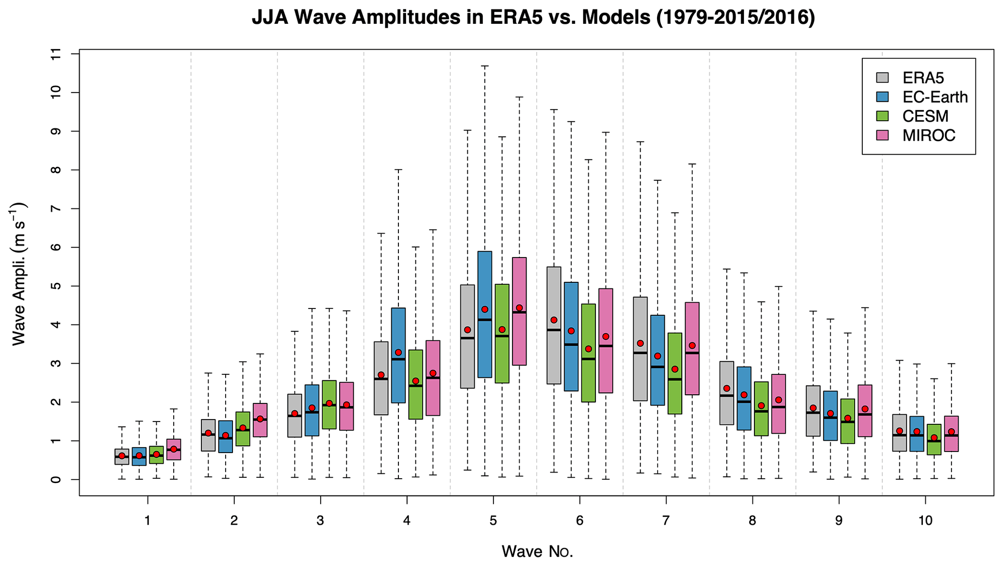
Figure 1Boxplot for wave amplitudes in AISI climatology runs for climate models EC-Earth, CESM, and MIROC as well as reanalysis data ERA5 for the period of June, July, and August in 1979–2015/2016. Red dots indicate the mean, and thick black lines represent the median. The lower hinge of each box is the Q1 quartile (25th), and the upper hinge is the Q3 quartile (75th). The upper and lower bars are based on 1.5 times the interquartile range (IQR) value. The outliers are not shown in the plot.
3.2 Wave phase-locking behaviors
Following Kornhuber et al. (2020), we use 1.5 SD above the mean wave amplitude as a threshold to define high-amplitude wave events to analyze phase-locking behavior of high-amplitude waves 5–8. The phase positions of high-amplitude episodes are shown in Fig. 2. In ERA5 waves have inherent phase-locking properties, especially for waves 5 and 7, as visible by a single peak in the probability density function. This is consistent with the work from Kornhuber et al. (2019), who used different reanalysis data, i.e., NCEP-NCAR (Kalnay et al., 1996). Also, in the NCEP-NCAR reanalysis data, waves 6 and 8 do not really show a preferred phase position. In our experiments, across all three models, strong phase-locking behavior is detected for wave 7. For wave 5, two models (CESM and MIROC) show phase locking that is comparable to ERA5; however EC-Earth underestimates the peak and thus the strength of phase locking.
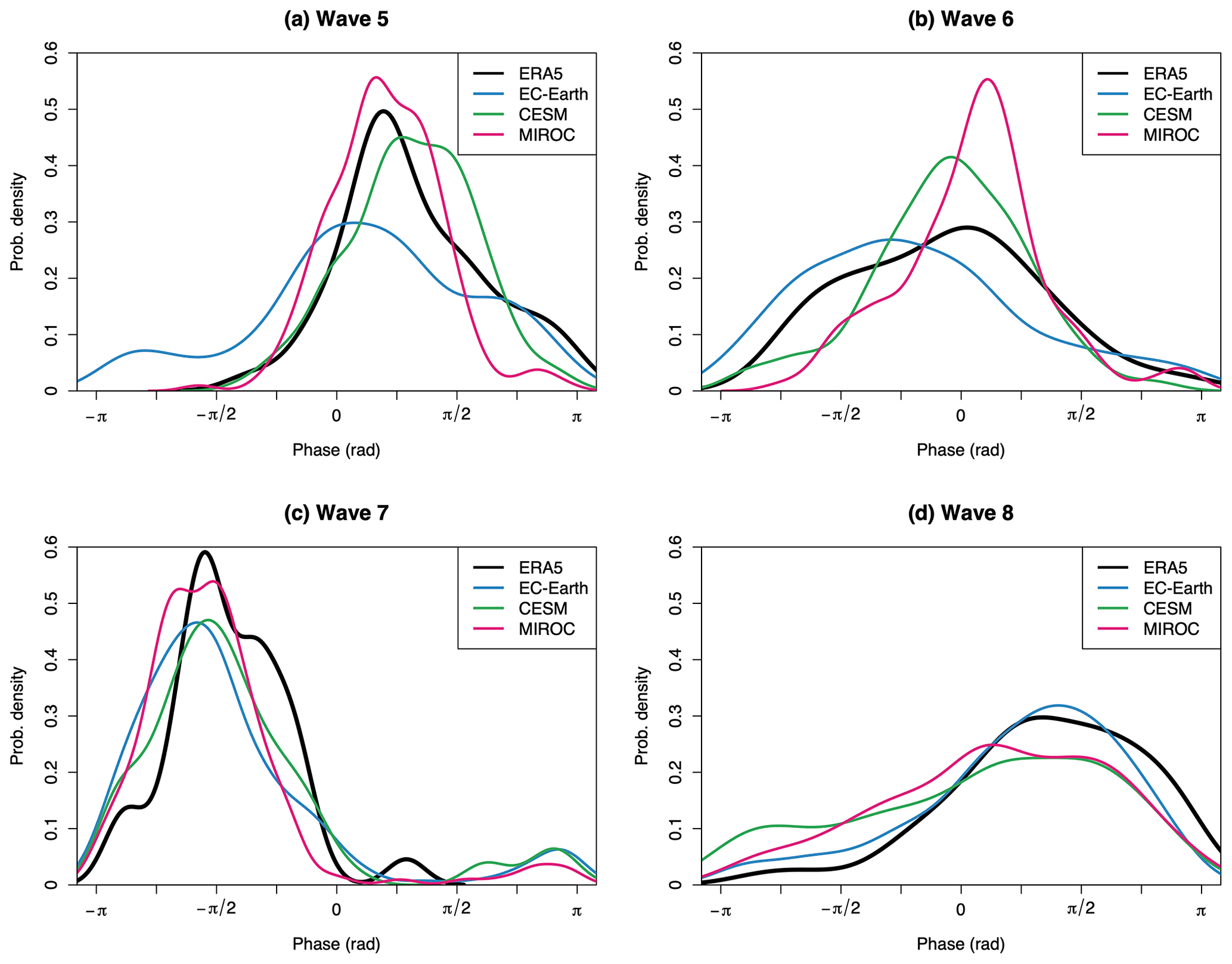
Figure 2Phase locking of Rossby waves for JJA ERA5 and model waves 5–8 in control run AISI for high-wave-amplitude episodes (> 1.5 SD). (a–d) Probability density functions of the phase positions of waves 5–8 in ERA5, EC-Earth, CESM, and MIROC during JJA for the period of 1979–2015/2016: wave 5 (a), wave 6 (b), wave 7 (c), wave 8 (d). The bandwidths for ERA5 and models are as follows. (a) Wave 5: 0.35(ERA5), 0.40 (EC-Earth), 0.25 (CESM), 0.22 (MIROC); (b) wave 6: 0.53 (ERA5), 0.45 (EC-Earth), 0.30 (CESM), 0.25 (MIROC); (c) wave 7: 0.25 (ERA5), 0.29 (EC-Earth), 0.27 (CESM), 0.22 (MIROC); (d) wave 8: 0.49 (ERA5), 0.39 (EC-Earth), 0.52 (CESM), 0.46 (MIROC).
ERA5 shows no phase locking for wave 6 and wave 8 but rather only a mild preference for some phase positions. The models capture this, with only MIROC showing fairly pronounced phase-locking behavior for wave 6. Detailed histograms comparing the models with ERA5 are provided in Fig. B2.
3.3 High-amplitude wave episodes and their surface imprint
We find that the preferred phase position of waves 5 and 7 is reasonably well represented in models. We next analyze high-amplitude episodes (i.e., those exceeding 1.5 SD) in more detail. The wave episode occurrence is computed as the percentage of weeks showing high-amplitude-wave episodes during the 1979 to 2015/16 summer. For ERA5, this is the case for 8.1 % and 7.1 % of all weeks for wave-5 and wave-7 events, respectively. The occurrence frequencies are quite comparable for the models: 7.7 % (EC-Earth), 8.0 % (CESM), and 7.9 % (MIROC) for wave 5 and 8.1 % (EC-Earth), 7.8 % (CESM), and 8.0 % (MIROC) for wave 7. Figures 3 and 4 show the upper-level meridional wind (v at 250 hPa, absolute field) and anomalies of near-surface temperature (t2m), precipitation (prcp), and sea level pressure (mslp) during high-amplitude events in ERA5 (Figs. 3a and 4a). The same variables are shown for the free-running atmosphere and soil moisture (AISI) experiments using the three climate models (Figs. 3b–d and 4b–d). Extended analysis for other wavenumbers revealed that the evaluated models are capable of reproducing the high-amplitude Rossby waves 4 to 8 and their associated surface anomalies reasonably well (Figs. B3–B5). The results imply that the model is able to reproduce summertime surface anomalies associated with different wavenumber episodes. Using anomalies for the upper-level meridional winds, in contrast to absolute v250, gives consistent results (compare Figs. 3 and 4 and Figs. B10 and B11, respectively). Furthermore, Figs. B12 and B13 show that the composite anomalies for v250, t2m, and mslp are significant for both waves 5 and 7, accounting also for the false discovery rate (FDR; Benjamini and Hochberg, 1995).
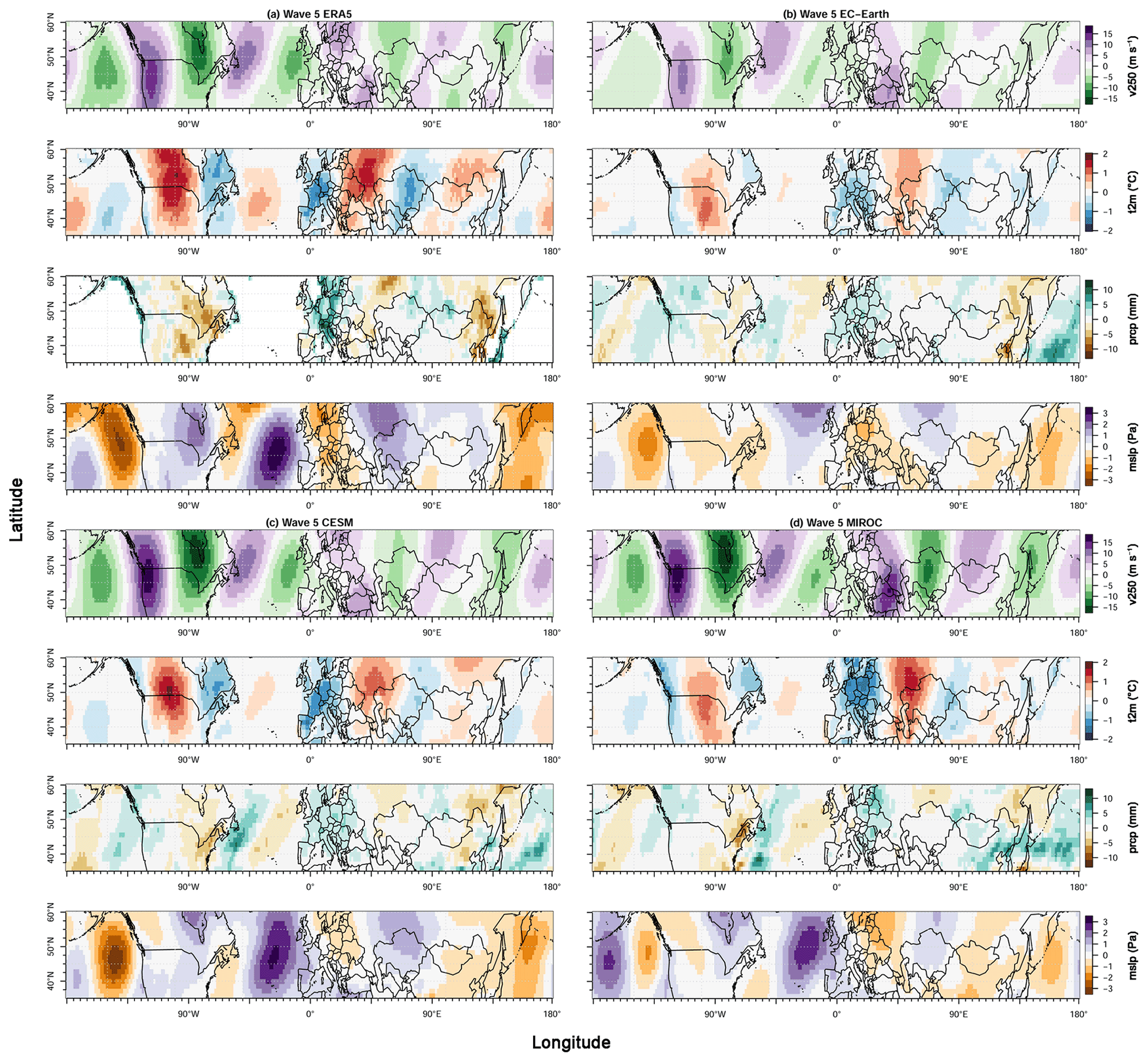
Figure 3Composite anomaly plots of weeks with high-amplitude wave-5 episodes for meridional wind velocity at 250 hPa (v250, absolute field), near-surface temperature (t2m, anomaly), precipitation (prcp, anomaly), and sea level pressure (mslp, anomaly) in ERA5 (a), EC-Earth (b), CESM (c), and MIROC (d) based on the AISI control runs.
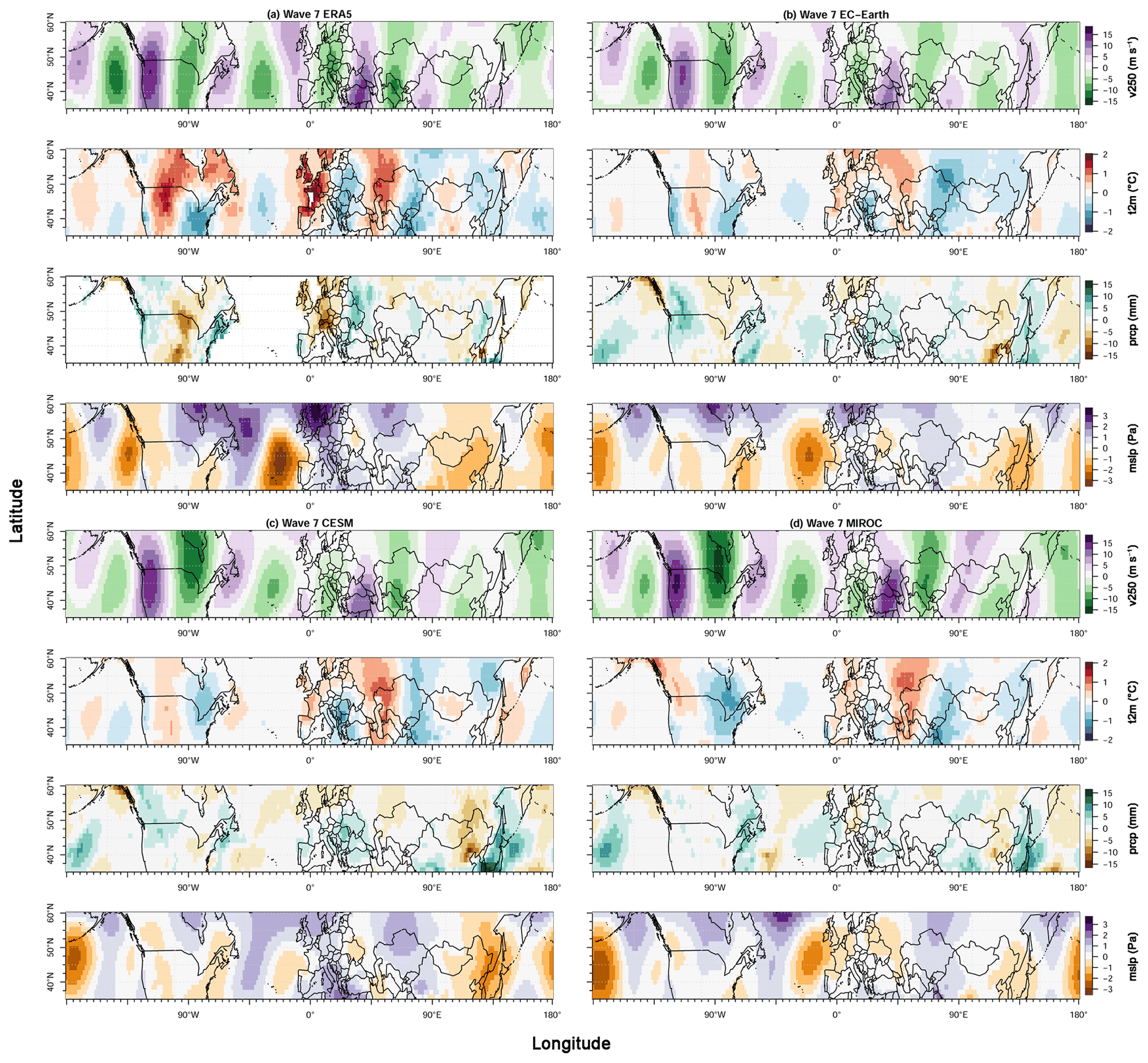
Figure 4Composite anomaly plots of weeks with high-amplitude wave-7 episodes for meridional wind velocity at 250 hPa (v250, absolute field), near-surface temperature (t2m, anomaly), precipitation (prcp, anomaly), and sea level pressure (mslp, anomaly) in ERA5 (a), EC-Earth (b), CESM (c), and MIROC (d) based on the AISI control runs.
Additionally, to quantify the bias of all models and to visualize how close the models are to the ERA5 reanalysis data, we present our findings in a Taylor diagram (Taylor, 2001) for wave 5 (Fig. 5) and wave 7 (Fig. 6). A Taylor diagram presents three key statistics in one single plot: the Pearson correlation between the observed and modeled spatial pattern; the centered root mean square error (RMSE) of the modeled field compared to observed; and the normalized spatial standard deviation of the modeled field, as compared to observed. Thus, v250 during high-amplitude wave episodes and t2m, prcp, and mslp anomalies from the different models are plotted in the Taylor diagram, showing their correspondence to ERA5 reanalysis data.
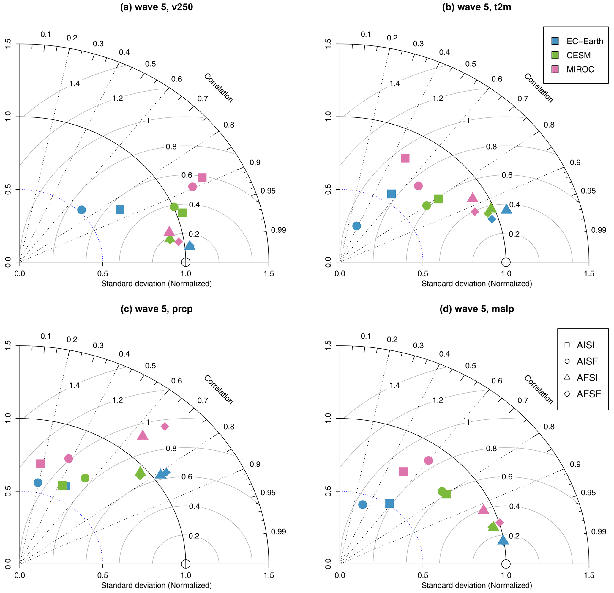
Figure 5Taylor diagram for all experiments in models compared to ERA5 for wave-5 events and episodes. For (a) v250, (b) t2m, (c) prcp, and (d) mslp, the Taylor diagram presents three statistics for each model and each experiment: the Pearson correlation (dashed lines), the RMSE (gray contours), and the normalized spatial standard deviation (solid black contours).
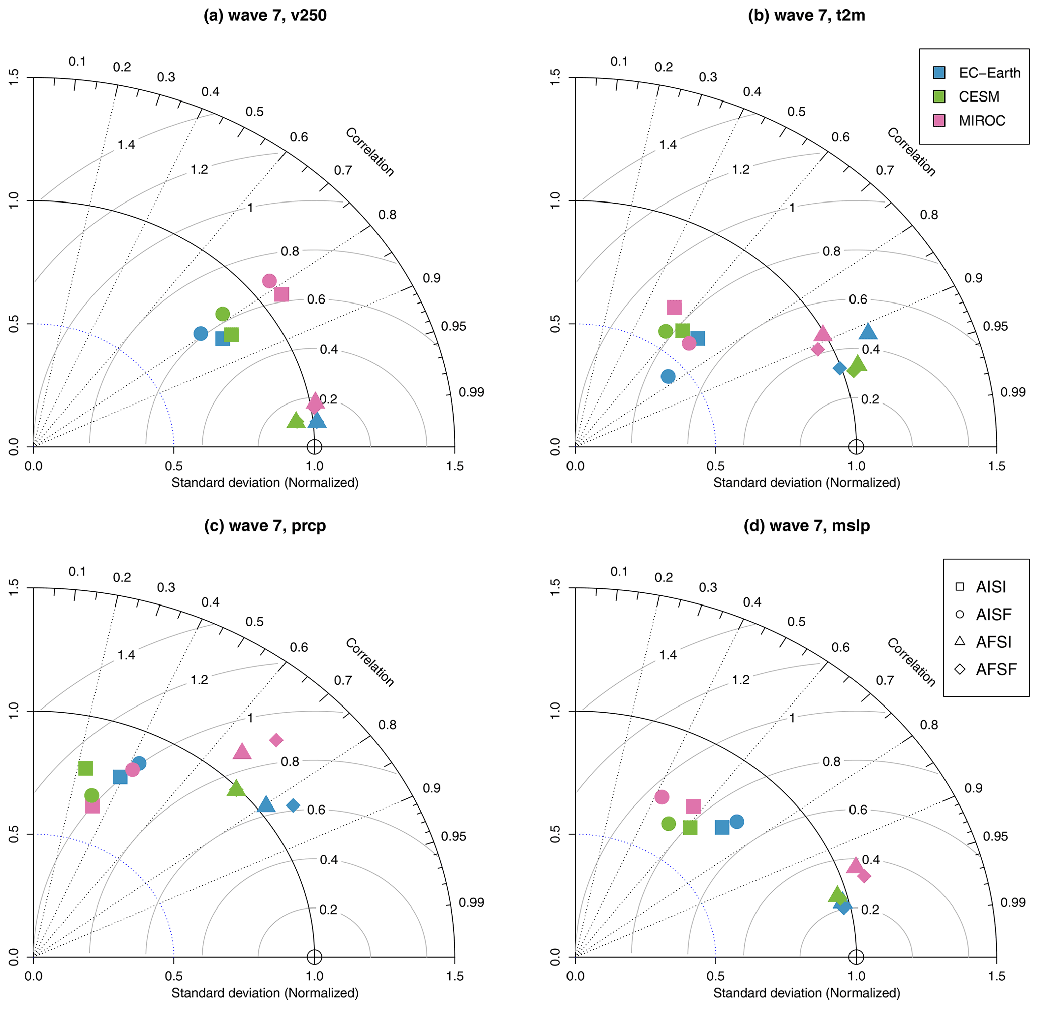
Figure 6Taylor diagram for all experiments in models compared to ERA5 for wave-7 events and episodes. For (a) v250, (b) t2m, (c) prcp, and (d) mslp, the Taylor diagram presents three statistics for each model and each experiment: the Pearson correlation (dashed lines), the RMSE (gray contours), and the normalized spatial standard deviation (solid black contours).
All models are able to capture the mean upper-level circulation patterns reasonably well for wave 5 with correlations for v250 of 0.86 (EC-Earth), 0.95 (CESM), and 0.88 (MIROC) (Fig. 5 and Table A1). This is consistent with our findings from Figs. 1 and 2. For the wind speed anomalies, CESM and MIROC have similar magnitudes compared to ERA5 data, whereas the signal from EC-Earth is weaker. The normalized standard deviation (n.s.d.) for EC-Earth is 0.70, for CESM it is 1.04, and for MIROC it is 1.24. This also holds for t2m anomalies during wave-5 events as all models are able to reproduce the patterns found in ERA5, such as the continental-scale patterns of positive and negative temperature anomalies for central North America (+), western Europe (−), and central Europe (+). However, the strength of the patterns is weaker in EC-Earth, especially for eastern Eurasia. The correlations of the t2m anomalies are substantially smaller for EC-Earth (0.55) and MIROC (0.48) than for CESM (0.81). As for prcp, all model correlations are below 0.50, with MIROC showing the lowest correlation (0.18), followed by CESM (0.43) and EC-Earth (0.46). The correlation values for mslp in models vary from 0.52 (MIROC) and 0.58 (EC-Earth) to 0.80 (CESM). As for the multi-model mean (MMM) n.s.d. of the different examined variables, there is a decline from v250 (0.99) to the surface variables t2m (0.71), mslp (0.69) and prcp (0.63). Thus, surface anomalies are consistently too weak. Both reanalysis data and models show strong positive anomalies in sea level pressure in the eastern basin of the Atlantic Ocean (west coast of Europe) during wave-5 episodes (Fig. 3).
For wave-7 episodes, the upper-level circulation patterns compare well to ERA5 data as shown by the field correlations in Table A1: 0.84 (EC-Earth), 0.84 (CESM), and 0.82 (MIROC). Again, this confirms that the models give a satisfactory performance in producing correct upper-level circulation patterns during high-amplitude wave episodes. This thus again indicates that models capture phase locking well. Correlations for surface variables are lower, with t2m correlation of 0.70 (EC-Earth), 0.63 (CESM), and 0.53 (MIROC). The positive t2m anomalies are quite pronounced in the regions of central North America, western Europe, northern Europe, and central Eurasia. All models are able to reproduce the sign of t2m anomalies in these regions but with smaller magnitudes than in ERA5. The n.s.d. values of the t2m anomalies are 0.62 (EC-Earth), 0.61 (CESM), and 0.67 (MIROC) (Table A2). The large-scale precipitation anomaly patterns in EC-Earth relate well to WFDE5_CRU data for North America, whereas in both CESM and MIROC there is more noise. The correlation of precipitation anomalies is 0.32 in the MMM. The large-scale patterns of mslp during wave-7 episodes match relatively well with ERA5 data, with a MMM correlation value of 0.63. On the eastern side of the Atlantic Ocean (west coast of Europe), strong negative mslp anomalies can be seen for the wave-7 composites, which is opposite to the wave-5 signal here. Also, positive mslp anomalies are found during wave-7 episodes on the east coast of North America (Fig. 4), whereas the location shows negative anomalies during wave-5 episodes (Fig. 3).
One common finding from both wave-5 and wave-7 episodes is that the biases (n.s.d. ≥ 0.75) in upper-level circulation are smaller compared to more pronounced biases in the t2m, prcp, and mslp surface anomalies. All models substantially underestimate the magnitude of t2m, prcp, and mslp anomalies associated with wave-5 and wave-7 episodes, typically by a factor of 1.5 (Table A4).
3.4 Investigating sources of model biases
Next, we aim to infer the biases from composites of anomalies shown in Figs. 3 and 4 for the upper-level wind and surface fields. As defined in the “Data and methods” section, the bias maps were computed as the differences between the selected variables' anomalies in the models and in the ERA5 reanalysis data during high-amplitude wave-5 and wave-7 events. Note that the biases that we refer to in surface variables are the biases of the anomalies instead of the absolute bias of the models. Here we present and describe the EC-Earth bias maps only. Equivalent plots for the other two models, with qualitatively similar outcomes, can be found in Figs. B6 to B9.
Here, we also employ the different nudged experiments: AISF (soil moisture prescription), AFSI (upper-level atmosphere nudging), and AFSF (nudging both) (see “Data and methods” section above for details). Overall, when nudging both the atmosphere and soil moisture, the residual bias B_res is, as expected, negligible. This is true for both wave-5 and wave-7 episodes in all models and all analyzed variables (Figs. 7 and 8).
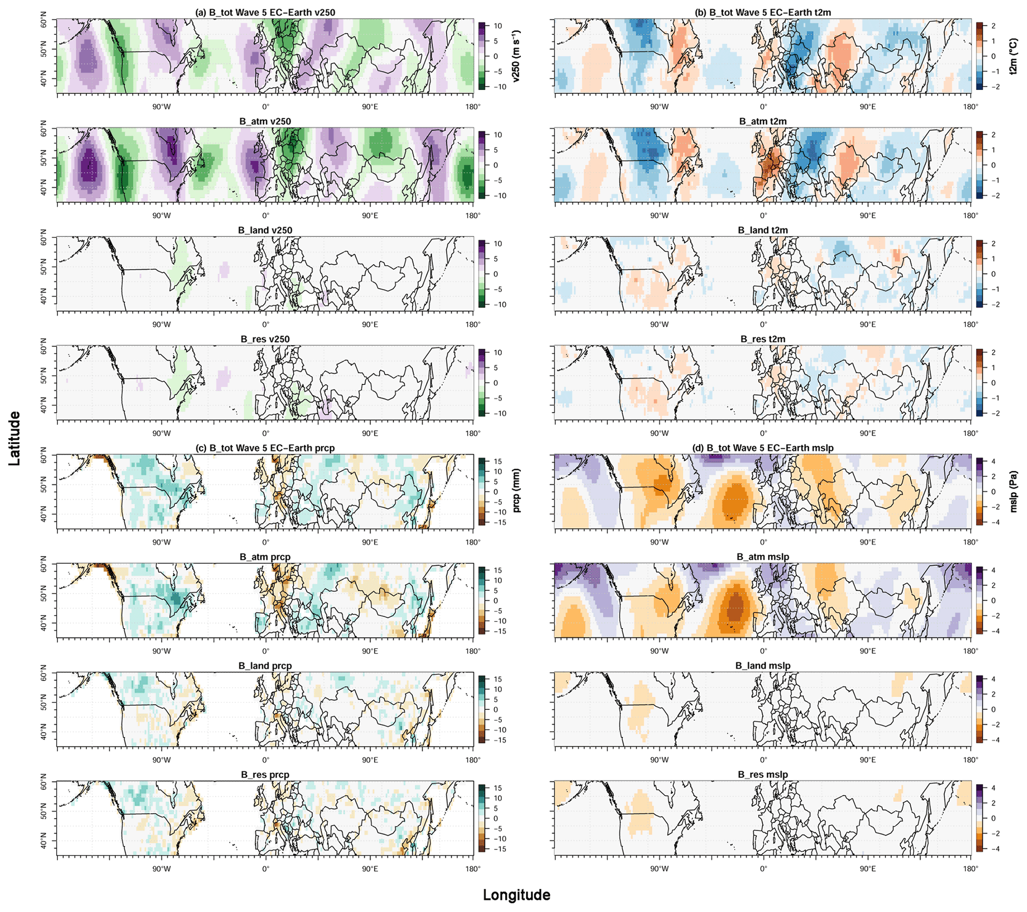
Figure 7Bias plots for high-amplitude wave-5 events and episodes in different experiments for EC-Earth. Total bias (B_tot), atmospheric bias (B_atm), land–atmosphere interaction bias (B_land), and residual bias (B_res) for meridional wind velocity at 250 hPa (a), surface temperature (b), precipitation (c), and sea level pressure (d).
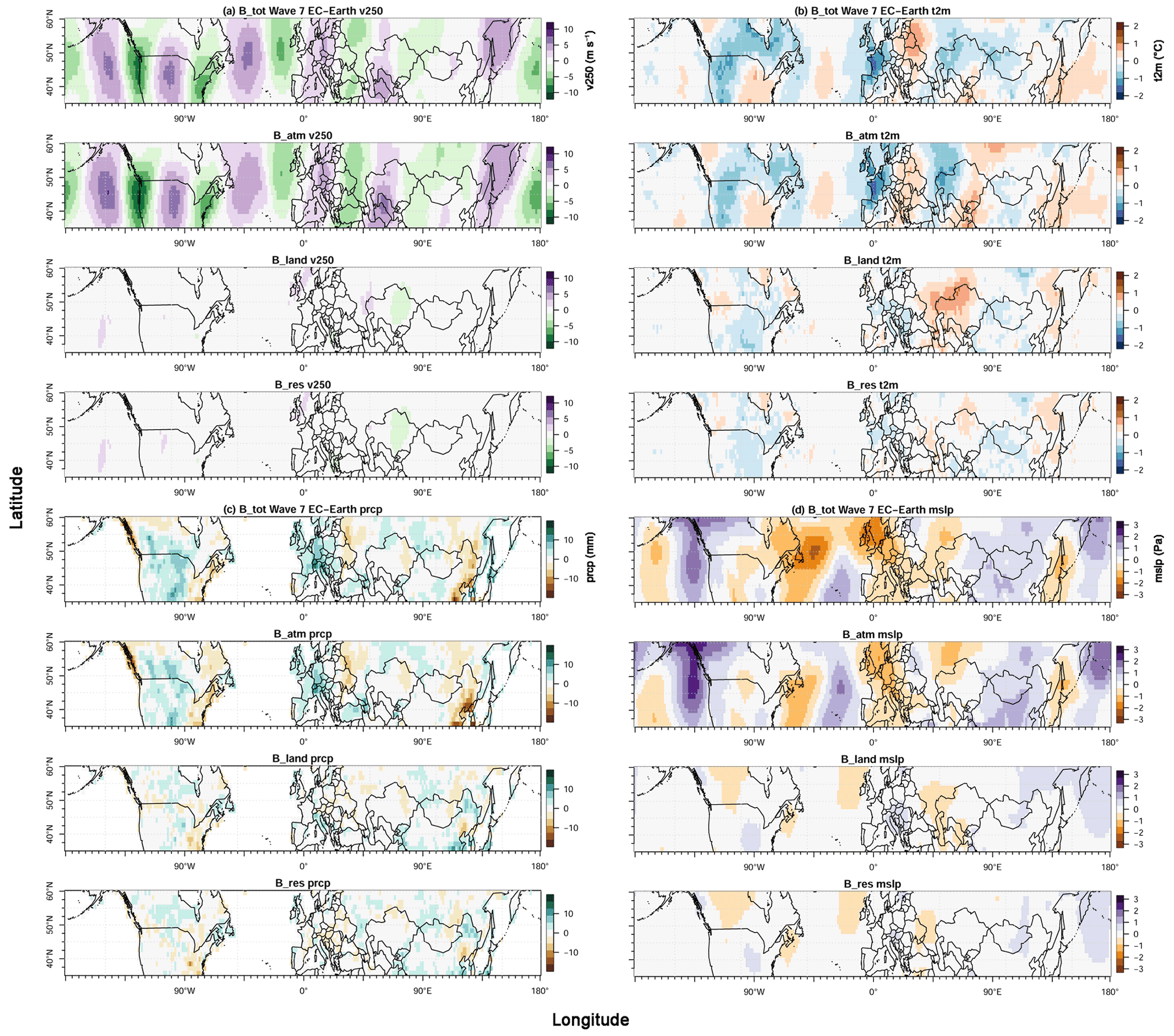
Figure 8Bias plots for high-amplitude wave-7 events and episodes in different experiments for EC-Earth. Total bias (B_tot), atmospheric bias (B_atm), land–atmosphere interaction bias (B_land), and residual bias (B_res) for meridional wind velocity at 250 hPa (a), surface temperature (b), precipitation (c), and sea level pressure (d).
By nudging the atmosphere, the bias from the atmospheric part (B_atm) is (of course) almost completely removed for the v250 anomaly across all models (see Fig. 7a, B_land). More interestingly, Fig. 7b shows that most of the EC-Earth t2m anomaly bias is also removed when we nudge the upper-level atmosphere. Thus, the total bias (B_tot) in t2m is almost completely explained by the upper-level atmospheric bias (B_atm), and the contribution of the land–atm bias (B_land) is negligible (Fig. 7b).
As for wave 5, the free-running EC-Earth (AISI) has a relatively smaller bias in v250 (blue square in Fig. 5a), with a correlation of ∼ 0.9, a RMSE of ∼ 0.5, and a n.s.d. of ∼ 0.7 compared to the biases in the surface variables. In other words, the pattern is very similar but with a somewhat underestimated strength in terms of wind speed. Still the bias in t2m (B_tot, blue square in Fig. 5b) is substantially larger, with a correlation of ∼ 0.6, RMSE ∼ 0.9, and n.s.d. ∼ 0.6. Thus, the t2m anomaly is underestimated by about a factor of 1.7 (n.s.d. ∼ 0.6). This substantial bias in t2m is almost completely removed when nudging the upper-level wind field, i.e., removing the bias in v250. This is shown by the blue triangle in Fig. 5b for AFSI, which has a correlation of 0.94, a RMSE of 0.36, and a n.s.d. of 1. As can be seen in Fig. 5, the other models behave qualitatively in a similar way, with substantial biases in near-surface temperature (in AISI, squares in Fig. 5b) which are largely removed when the bias in upper-level wind is removed by nudging (in AFSI, triangles in Fig. 5b).
Errors in precipitation anomalies are not fully removed when nudging upper-level circulation. Figure 5c shows some reduction in the overall magnitude of errors in precipitation; in particular the field correlation and n.s.d. improve by almost a factor of 2 (Fig. 5c). Still the RMSE only marginally reduces when upper-level atmospheric nudging is applied. Biases in sea surface pressure anomalies, on the other hand, are almost completely removed with nudging (Fig. 5d).
Similarly, for wave-7 episodes, Fig. 8b confirms our finding that nudging the upper-level atmosphere alone reduces the bias in surface temperature dramatically. Therefore, the total bias (B_tot) in t2m can be explained to a large extent by B_atm, and again the land contribution to the total bias is insignificant (Fig. 8b). Specifically, with the aid of a Taylor diagram (Fig. 6b and d), there is a clear improvement when nudging the atmosphere (AFSI) as compared to the control run AISI and the prescribed soil moisture run AISF. The t2m bias still remains substantial when prescribing the soil moisture. The actual n.s.d. and RMSE values for v250 in AFSI are 1.0 and 0.10, compared to 0.8 and 0.55 for AISI, respectively. Figure 6 also exhibits that CESM and MIROC have similar characteristics, with substantial biases of t2m and mslp that are effectively removed by upper-level atmospheric nudging. Still in EC-Earth, for t2m, n.s.d. improves from 0.62 to 1.1 and mslp from 0.74 to 1.0. Thus, by nudging the upper-level atmosphere the surface variables get the correct magnitude. Figure 6c also shows that the spatial pattern correlation improves for prcp from 0.39 for the free-running AISI run to 0.80 in the AFSI run. Another interesting observation obtained from comparing wave-5 and wave-7 Taylor diagrams is that the models are more clustered for all variables for wave 7 compared to wave 5.
In general, nudging the soil moisture does not affect the upper-atmospheric flow. AISF runs have similar biases in terms of correlation, n.s.d., and RMSE for t2m and prcp compared to AISI across the different models. The same conclusion stands for the AISF and AFSI runs for prcp and mslp. The aforementioned observations are location-specific as one component within a climate model might, erroneously, be tuned in such a way that it compensates for biases in other components of the climate model. If so, nudging only that component would not reduce the overall bias. In this case, prescribing only the soil moisture part does not guarantee a reduction in the overall bias.
4.1 Discussion
Large atmospheric circulation patterns, especially amplified wave-5 and wave-7 circumglobal Rossby waves, play an important role in climate variability and can trigger and maintain persistent extreme events such as heat waves and prolonged precipitation periods during the summer months. In this study, we demonstrate that individual Fourier modes are well captured in different climate models in terms of their climatology and variability. The phase-locking behavior, in particular for wave 5 and wave 7, is captured. Both amplitude and week-to-week variability, in terms of standard deviations, are reasonably well reproduced in all models for all relevant wavenumbers. The composites and bias metrics for the upper-level wave (v250) during wave-5 and wave-7 episodes show that the wave's amplitude and pattern are well captured. Although the upper-level wind flows are satisfactorily reproduced across all models, their associated anomalies in surface variables (temperature, precipitation, and sea level pressure) during high-amplitude wave-5 and wave-7 episodes are too weak. The MMM n.s.d.'s for t2m and prcp are typically underestimated by a factor of 1.5 in wave-5 and wave-7 episodes. These model biases can be largely corrected by nudging the upper-level atmosphere. For instance, the n.s.d.'s for the t2m, prcp, and mslp improve approximately by a factor in the range of 1.4 to 1.6 for wave-5 and wave-7 episodes. Such reductions in bias metrics are not observed when prescribing the soil moisture. This implies that when removing an unsubstantial bias in the upper-atmospheric levels (by nudging the circulation), this removes the relatively large biases in surface anomalies relevant for extremes. A full analysis of the underlying reasons is outside the scope of this paper, but here we discuss some potential mechanisms. First, nudging zonal (u) and meridional (v) winds in the upper atmosphere strongly constrains the large-scale vertical wind component (ω), which is a key input for cloud parameterization schemes. In models, large-scale vertical wind is primarily defined by divergence in the horizontal wind fields, ensuring mass conservation, and thus nudging u and v will also effectively nudge ω. Likewise, biases in u and v will propagate in ω and can then have a strong, possibly non-linear impact on the number of clouds in models (Satoh et al., 2019; Rio et al., 2019). Regions with anomalously high pressure associated with a quasi-stationary Rossby wave will have pronounced subsidence in ERA5, but this is likely too weak in the models as this subsidence might not be well represented in the models because of biases in the upper-level flow. As a consequence, the models might have hazier cloud conditions as compared to clear-sky conditions in ERA5. This would impact the surface by reduced shortwave radiation and hence less pronounced warm anomalies. Potential limitations in the cloud parametrization schemes could exacerbate this as models have difficulties reproducing clear-sky conditions (Lacagnina and Selten, 2014). The resolution for general circulation models (GCMs) often does not allow sub-grid-scale convective systems and their associated clouds to be resolved. More generally, particularly in mid-latitude continents, climatological biases in both clouds and precipitation persist in major GCMs (Rio et al., 2019). Specifically for EC-Earth, it has been shown that there are too many clouds in this model that are optically thick but too few clouds that are optically thin (Lacagnina and Selten, 2014). Thus, this way, a relatively small bias in the upper-level horizontal wind fields could propagate via vertical wind and cloud scheme into more substantial biases at the surface.
While previous work has indicated that soil moisture can have pronounced effects on quasi-stationary Rossby waves, including circumglobal waves (Koster et al., 2016; Teng et al., 2019), our analyses show that adjusting for soil moisture biases (by prescribing soil moisture) has little effect on the representation of circumglobal waves and their associated surface anomalies. These differences could arise from different timescales and/or experiment setups. Earlier studies focused mainly on monthly to seasonal mean responses, while we analyze weekly timescales. In addition, Teng et al. (2019) apply a very strong soil moisture anomaly by setting it to zero over the western US, a region to which the climatological circumglobal wave might be particularly sensitive. In contrast, in our prescribed soil moisture experiments, the soil moisture is set to more realistic values, substantially larger than zero, coming from the model's land component forced by atmospheric fields from reanalysis. Our experiments thus represent much smaller forcings than those of Teng et al. (2019).
To be clear, our results are not questioning the importance of soil moisture as a prime driver of summer surface temperature extremes in various regions throughout the mid-latitudes. Rather, our study shows that prescribing the soil moisture in the models has little effect on surface variables and upper-level variables during high-amplitude wave episodes. Several studies have shown that soil moisture can play an important role in maintaining large-scale circulation anomalies associated with extremely warm and dry conditions (e.g., Erdenebat and Sato, 2018). In particular, under future climate change reduced soil moisture can lead to a higher probability of heat waves in Europe during summer via interactions between the land surface and the atmosphere (e.g., Seneviratne et al., 2006). This, however, does not say anything about the imprint of soil moisture biases on biases in near-surface climate in relation to the Rossby wave events investigated in our study. Apparently, it is the state of the atmosphere, i.e., circulation or clouds and precipitation, that governs the model biases in near-surface climate and not so much the state of the land surface. Further, in the interpretation of our results, one should be aware that in our prescribed soil moisture runs (AISF/AFSF), we prescribe the “approximately observed” soil moisture conditions (and not, for example, soil moisture climatology). This implies that the turbulent heat fluxes in AISF/AFSF still depend on this prescribed soil moisture condition. This means that during, for example, the heat wave period in Russia in 2010, the prescribed soil moisture will be anomalously dry, which will result in strong sensible heat fluxes.
4.2 Limitations and outlook
As with any choice of circulation metrics, our approach based on Fourier analyses of the zonally oriented wave component has its limitations. This approach implies that if a particular wavelength is pronounced in only one part of the hemisphere, this can result in a high-amplitude fast Fourier transform (FFT) signal. Thus, high-amplitude waves (as defined by our metrics) do not necessarily have to be circumglobal. They can result from either a circumglobal wave pattern or a pronounced regional wave pattern. Still, the fact that we find pronounced and significant wave patterns in our composite analyses reveals that those reflect preferred wave positions. In particular, wave 5 and wave 7 are subject to this phase-locking behavior. Whenever those quasi-stationary waves grow in amplitude, they tend to do so in the same longitudinal phase position, thereby causing temperature and precipitation anomalies in the same geographical regions. This has been reported before for observational data, highlighting the risks this creates for multiple breadbasket failures (Kornhuber et al., 2020). The prime motivation of our study is to see how well climate models reproduce these waves, and to that end our FFT-based metric is useful. Further, the number of high-amplitude waves in ERA5 might be under-sampled, which might lead to inconsistencies between models and ERA5. Since we use five ensemble members for the AISI experiment, the number of data is larger by a factor of 5 for the models compared to ERA5. As for the atmospheric nudging experiments, from the vertical nudging profile, it can be observed that in CESM and MIROC, the nudging intensity is identical, whereas in EC-Earth the nudging strength is weaker between 700 and 400 hPa. However, we do not think that these differences between exact model setup and potential under-sampling in ERA-5 have a large effect on our main findings.
Our findings have implications for climate model projections of persistent summer weather extremes in the key affected regions. Kornhuber et al. (2020) identified hotspots that are affected by summertime amplified wave-5 (central North America, eastern Europe, and eastern Asia) and wave-7 (west-central North America, western Europe, and western Asia) patterns. These regions are sensitive to simultaneous heat extremes, and to exacerbate the situation, some identified regions are also considered to be global breadbasket regions. In summers when wave-5 or wave-7 events persist more than 2 weeks, the average reduction in crop production is 4 % and even up to 11 % on a regional level (Kornhuber et al., 2020). In our study, for wave-5 and wave-7 events, all the aforementioned key regions are identified in our three models in terms of positive near-surface temperature anomalies. This gives more confidence that those state-of-the-art climate models can be used to study present and future agricultural risks associated with such wave patterns. Since the strength of the near-surface temperature anomalies is underestimated, the climate models are likely to underestimate heat waves as well. A potential way to adjust for this is to establish statistical links between upper-level atmospheric flows to near-surface temperatures based on observational data, then use this statistical link to adjust the effect of upper-level atmospheric circulation changes in climate models under future scenarios for heat wave risks. This approach is likely to be fruitful as our analyses suggest that upper-level waves are well represented across models. In addition, it will be important to assess how upper-level wave patterns change under future greenhouse gas forcing, in terms of position, strength, and persistence, and how that would affect surface extremes.
Our validation study shows that upper-level wave characteristics are reasonably well reproduced in three GCMs in historic AMIP runs, with MMM of n.s.d. for wave-5 and wave-7 episodes being 0.99 and 0.91. Both the climatology and phase-locking behaviors are captured in models for wavenumbers 5 and 7 as the MMM correlation values are 0.90 and 0.83. Surface temperature anomalies associated with amplified wave-5 and wave-7 patterns are weaker in models as compared to ERA5 reanalysis data. This bias in surface temperature anomalies during high-amplitude wave-5 and wave-7 episodes is effectively removed when nudging the mid- to upper-level atmosphere.
In summary, for the meteorological variables analyzed in this study, we find that
-
overall, v250 is accurately represented, and precipitation has the largest biases for both wave-5 and wave-7 episodes;
-
prescribing soil moisture does not improve the representation of surface anomalies in t2m and prcp;
-
nudging the upper-level atmosphere indicates that this is likely the prime origin of surface anomaly biases; we observe significant improvements from AISI and AISF runs to AFSI runs across all models and all variables.
We conclude that the relatively pronounced bias in the surface anomalies for amplified wave episodes mainly originates from smaller biases in the upper-level atmospheric circulation. Our study suggests that climate models can be used to study present and future wave characteristics but that care should be taken when analyzing the associated surface extremes.

Table A2Summary of model standard deviation values. NORM: normalized model mean value.


Table A4Summary of multi-model mean Taylor diagram values (corr.: correlation).
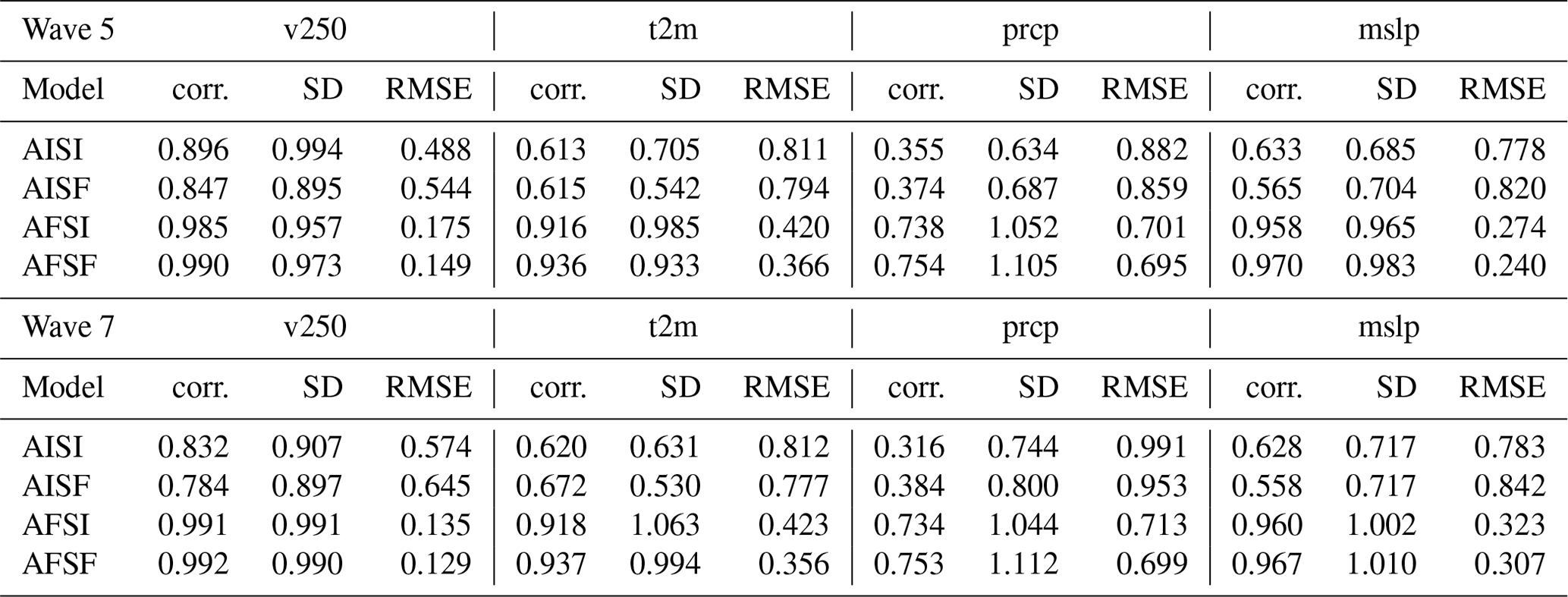
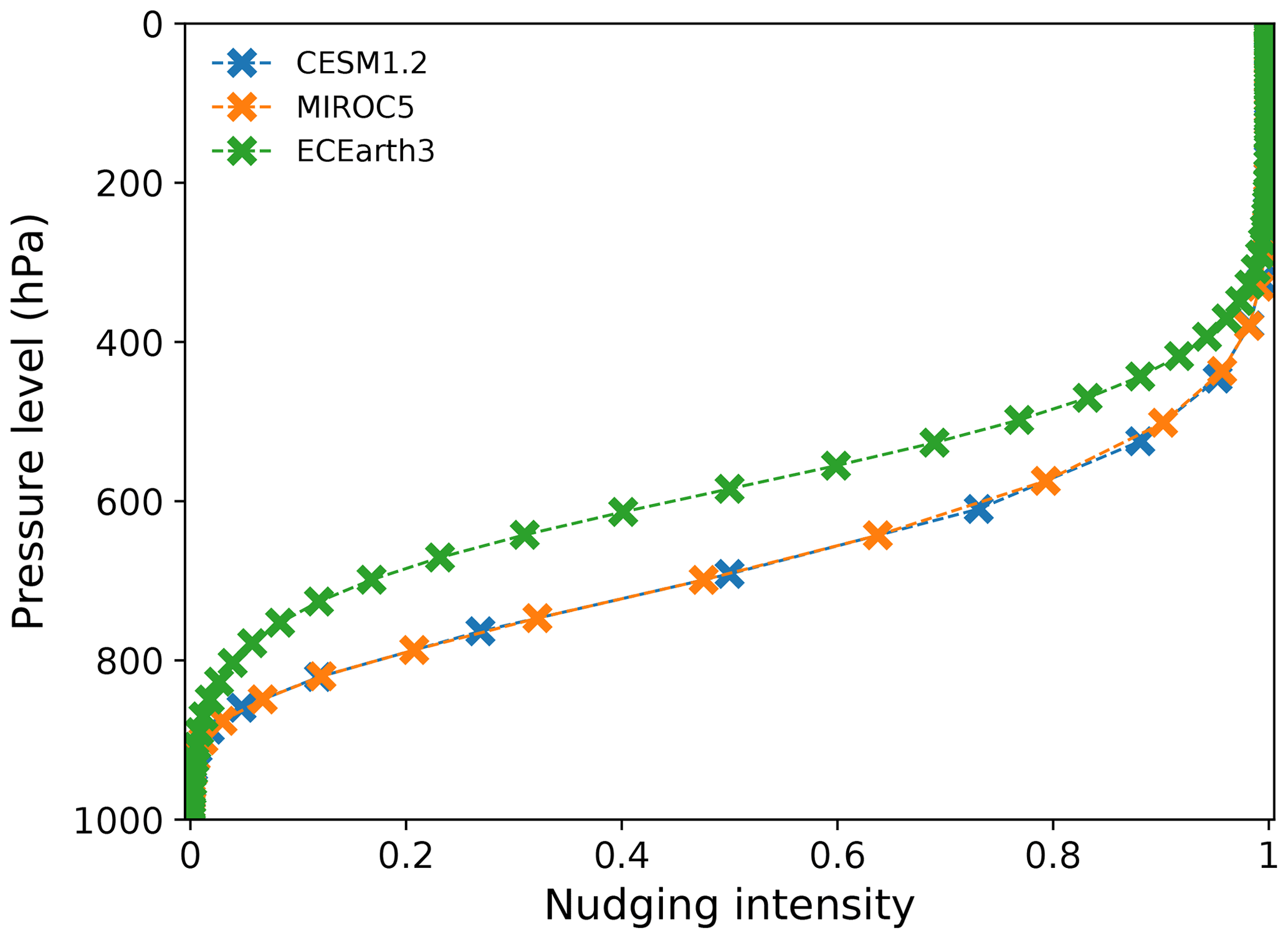
Figure B1Nudging profile for the three ExtremeX ESMs. The actual pressure levels are marked with an x and joined with lines. The nudging intensity is given from zero (no nudging) to one (fully nudged).
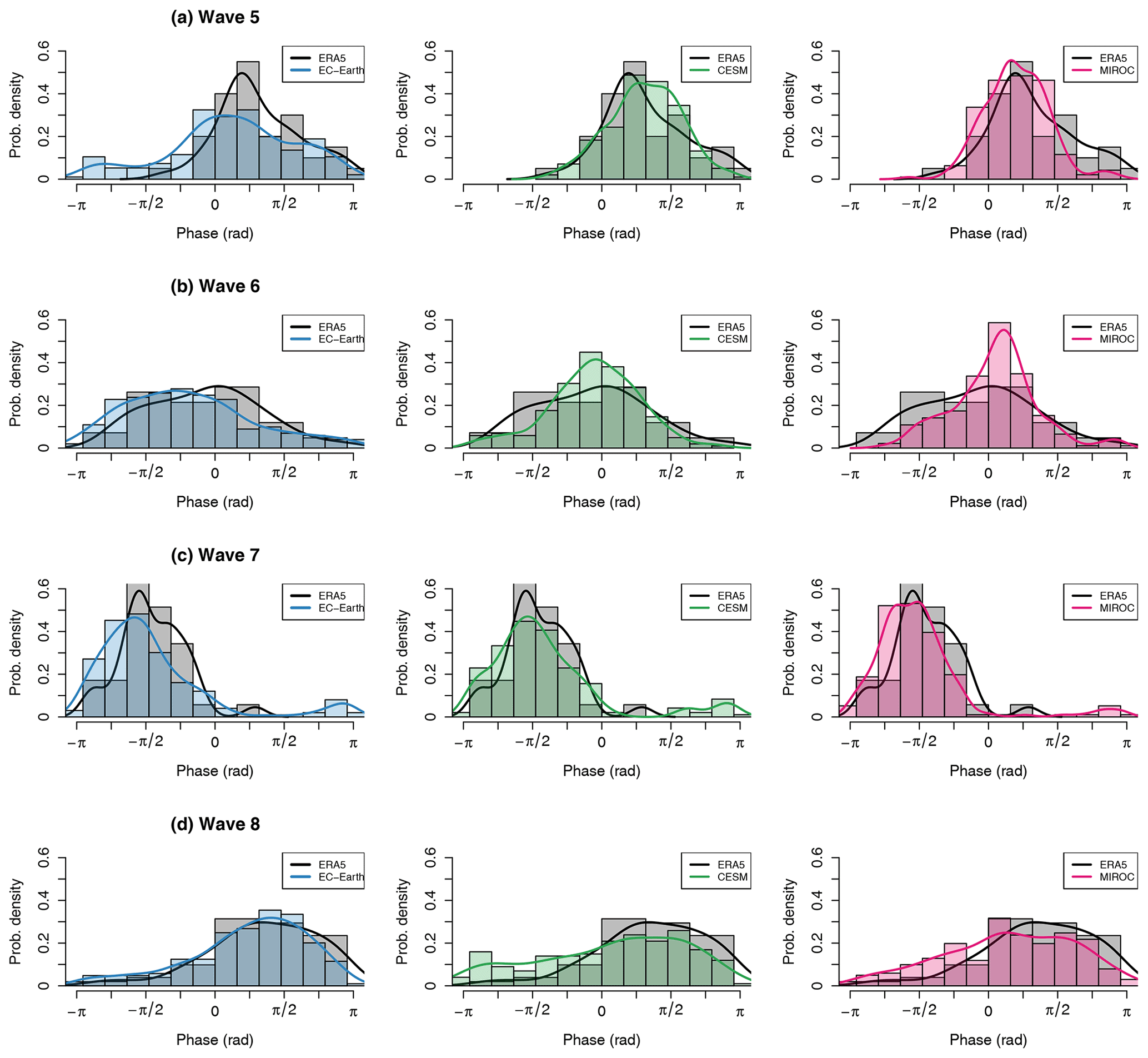
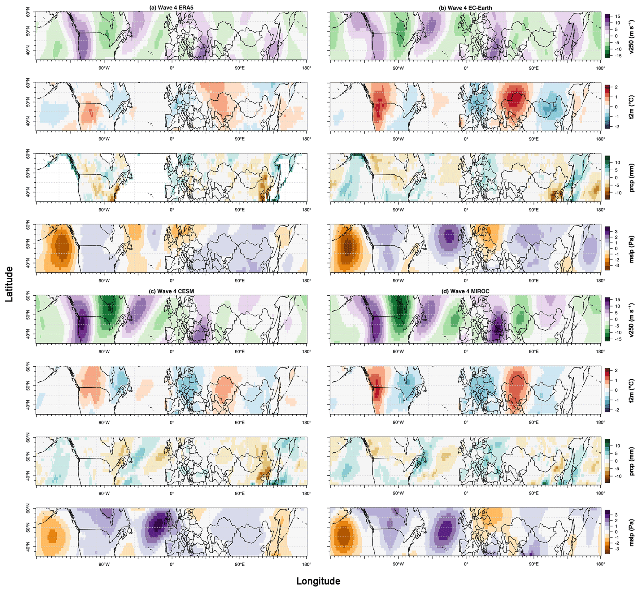
Figure B3Composite anomaly plots of weeks with high-amplitude wave-4 episodes for meridional wind velocity at 250 hPa (v250, absolute field), near-surface temperature (t2m, anomaly), precipitation (prcp, anomaly), and sea level pressure (mslp, anomaly) in ERA5 (a), EC-Earth (b), CESM (c), and MIROC (d) based on the AISI control runs.
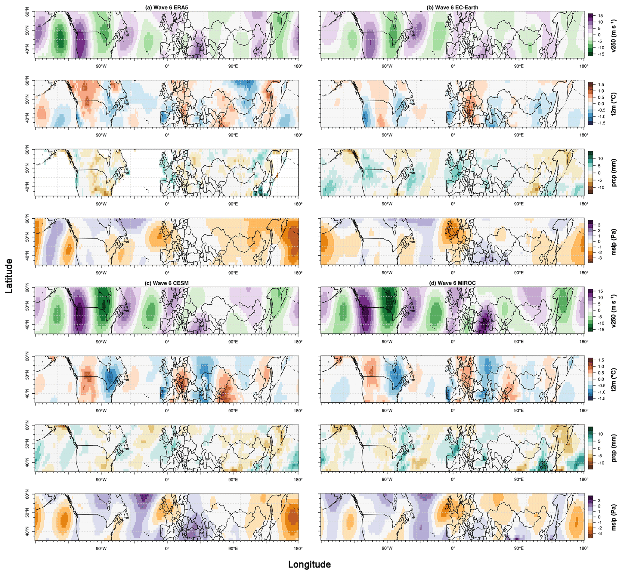
Figure B4Composite anomaly plots of weeks with high-amplitude wave-6 episodes for meridional wind velocity at 250 hPa (v250, absolute field), near-surface temperature (t2m, anomaly), precipitation (prcp, anomaly), and sea level pressure (mslp, anomaly) in ERA5 (a), EC-Earth (b), CESM (c), and MIROC (d) based on the AISI control runs.

Figure B5Composite anomaly plots of weeks with high-amplitude wave-8 episodes for meridional wind velocity at 250 hPa (v250, absolute field), near-surface temperature (t2m, anomaly), precipitation (prcp, anomaly), and sea level pressure (mslp, anomaly) in ERA5 (a), EC-Earth (b), CESM (c), and MIROC (d) based on the AISI control runs.

Figure B6Bias plots for high-amplitude wave-5 events and episodes in different experiments for CESM. Total bias (B_tot), atmospheric bias (B_atm), land–atmosphere interaction bias (B_land), and residual bias (B_res) for meridional wind velocity at 250 hPa (a), surface temperature (b), precipitation (c), and sea level pressure (d).
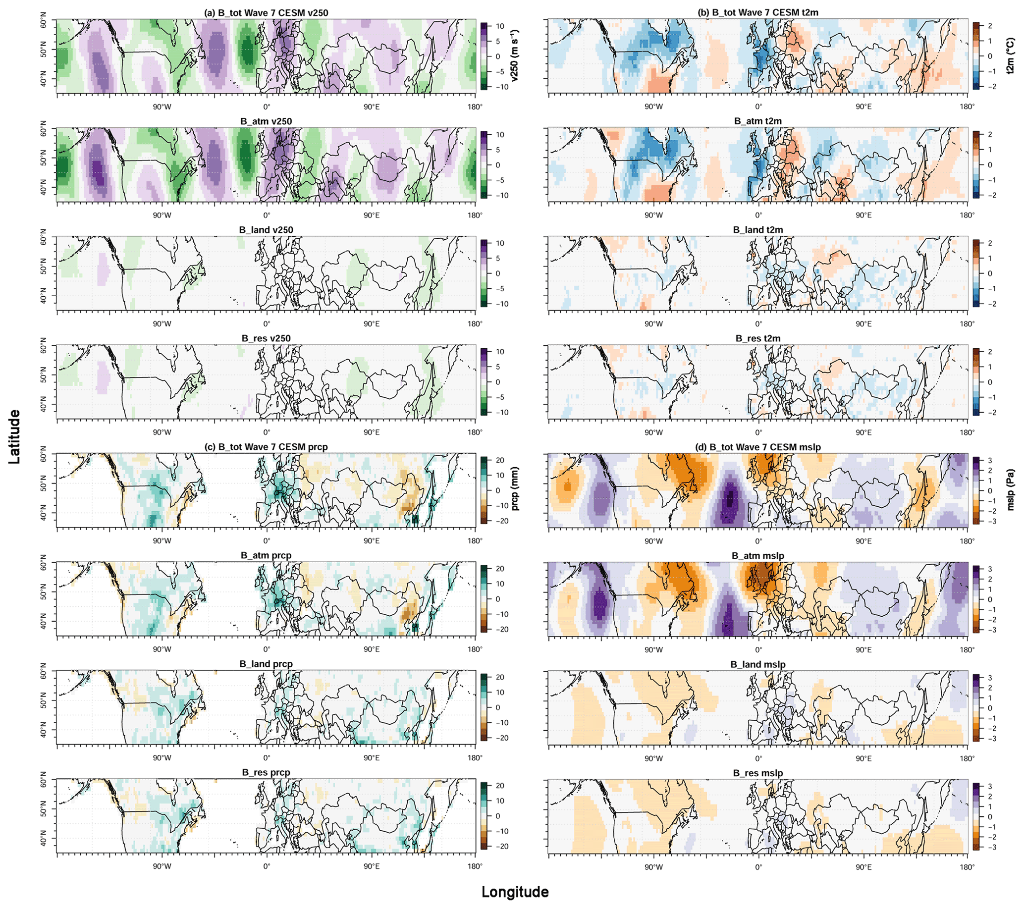
Figure B7Bias plots for high-amplitude wave-7 events and episodes in different experiments for CESM. Total bias (B_tot), atmospheric bias (B_atm), land–atmosphere interaction bias (B_land), and residual bias (B_res) for meridional wind velocity at 250 hPa (a), surface temperature (b), precipitation (c), and sea level pressure (d).

Figure B8Bias plots for high-amplitude wave-5 events and episodes in different experiments for MIROC. Total bias (B_tot), atmospheric bias (B_atm), land–atmosphere interaction bias (B_land), and residual bias (B_res) for meridional wind velocity at 250 hPa (a), surface temperature (b), precipitation (c), and sea level pressure (d).
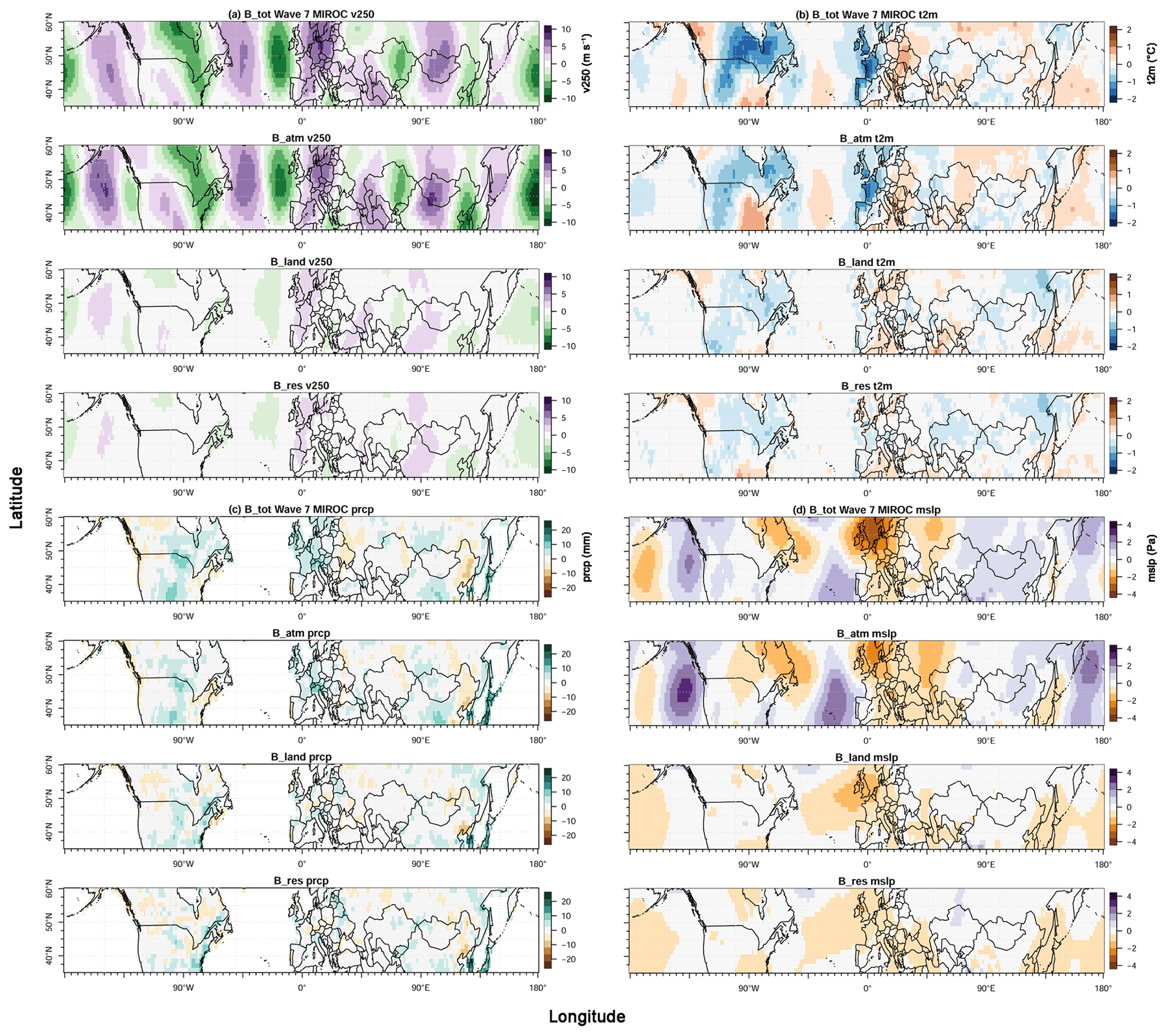
Figure B9Bias plots for high-amplitude wave-7 events and episodes in different experiments for MIROC. Total bias (B_tot), atmospheric bias (B_atm), land–atmosphere interaction bias (B_land), and residual bias (B_res) for meridional wind velocity at 250 hPa (a), surface temperature (b), precipitation (c), and sea level pressure (d).
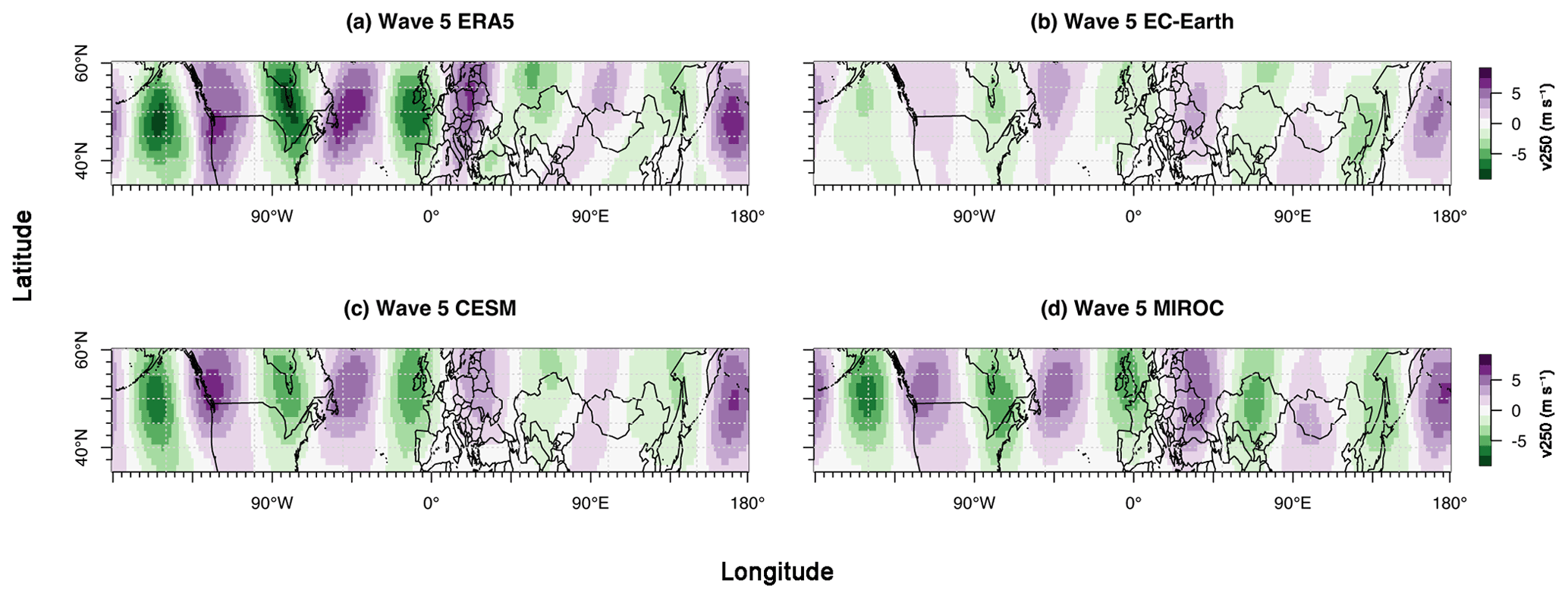
Figure B10Composite anomaly plots of weeks with high-amplitude wave-5 episodes for meridional wind velocity at 250 hPa (v250, anomaly) in ERA5 (a), EC-Earth (b), CESM (c), and MIROC (d) based on the AISI control runs.
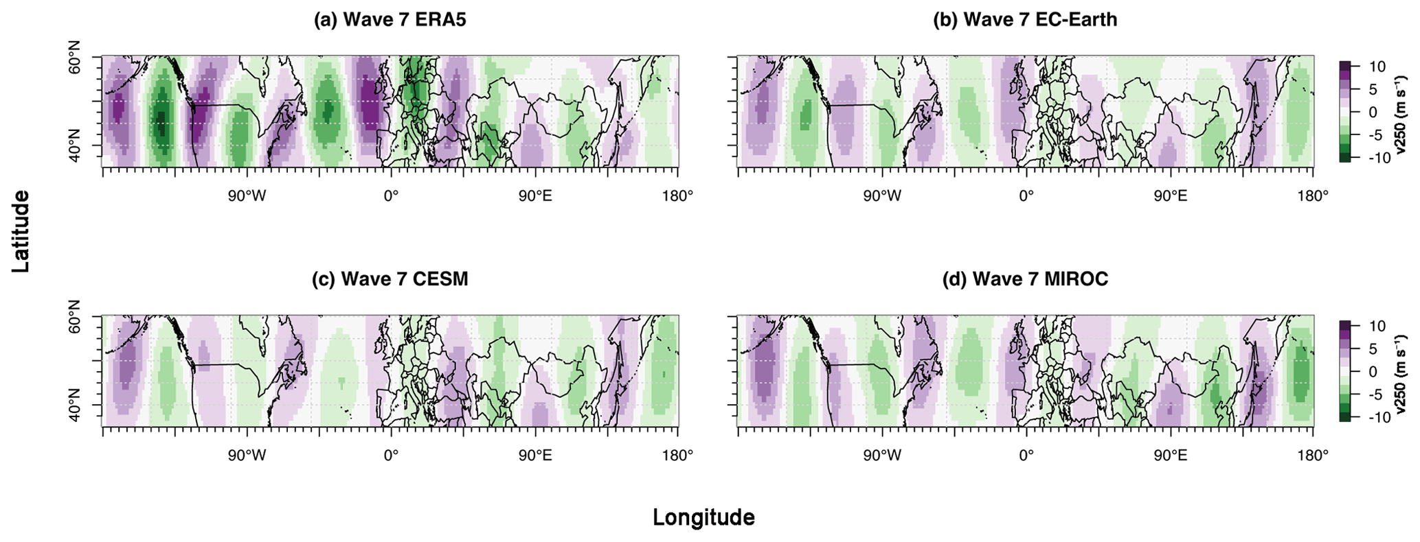
Figure B11Composite anomaly plots of weeks with high-amplitude wave-7 episodes for meridional wind velocity at 250 hPa (v250, anomaly) in ERA5 (a), EC-Earth (b), CESM (c), and MIROC (d) based on the AISI control runs.
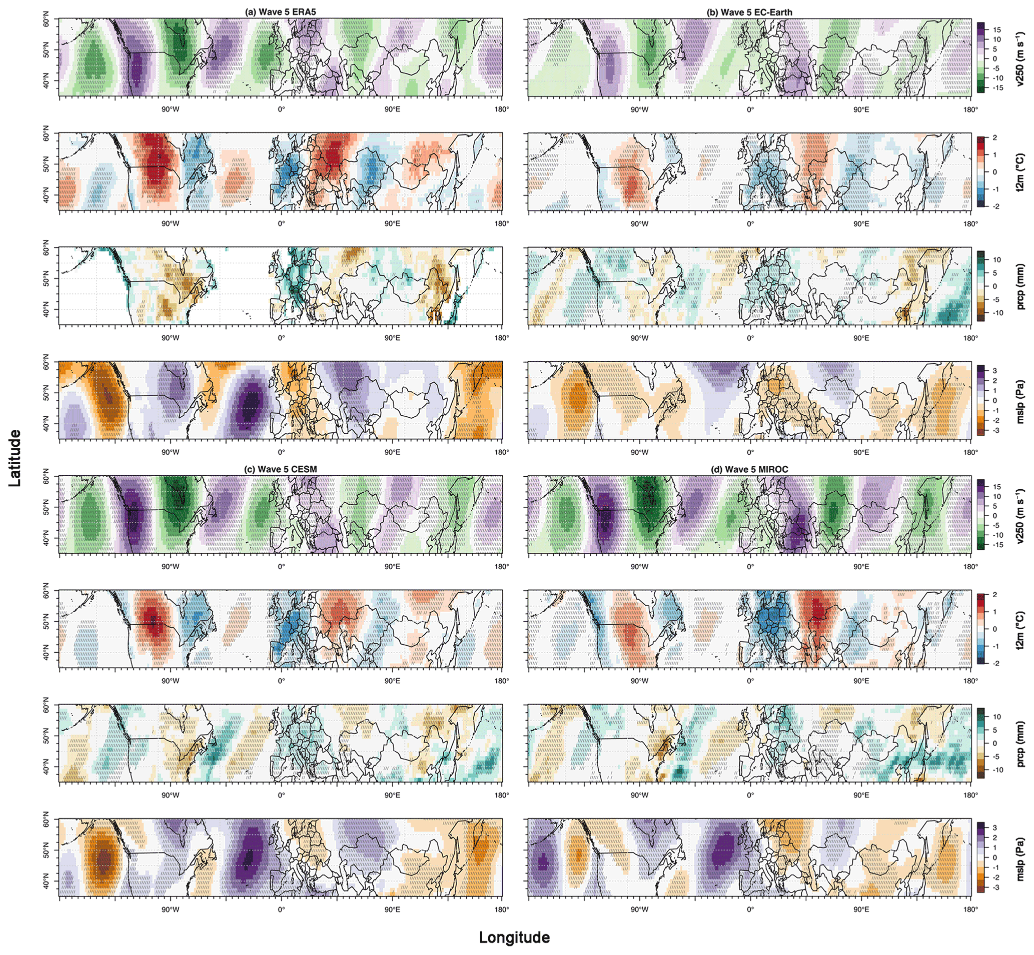
Figure B12Same as Fig. 3 but with significance test at 95 % confidence level applied. Values significantly exceeding the 95 % confidence level from composites between amplified and non-amplified periods are hatched.
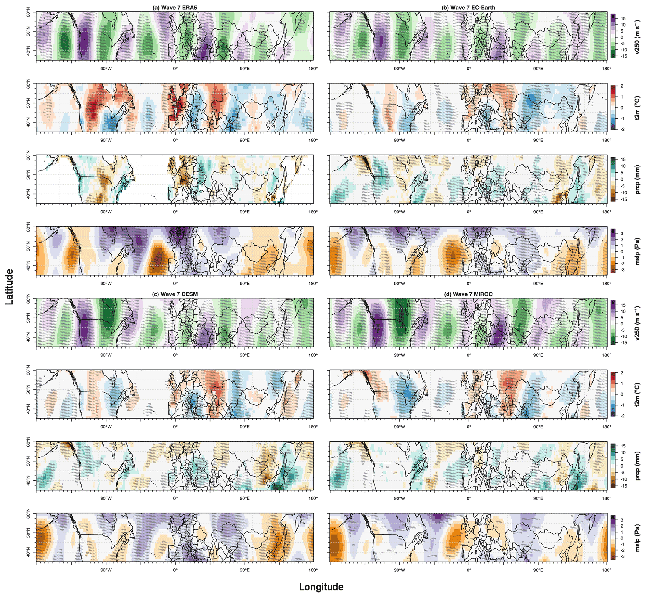
Figure B13Same as Fig. 4 but with significance test at 95 % confidence level applied. Values significantly exceeding the 95 % confidence level from composites between amplified and non-amplified periods are hatched.
The code and data can be made available by the authors upon request.
FL, DC, and FS designed the analysis with input from KK. FL ran the EC-Earth3 simulations with technical help from FS, WM, PLS, and TR. HS ran the interactive and atmosphere-nudged simulations with MIROC5. DT and HK ran the soil-moisture-nudged simulations with MIROC5. KW ran the CESM 1.2 model simulations, and SIS helped in the interpretations of these experiments. FL analyzed the results from all models. All authors contributed to the discussion of results. FL wrote the first draft, and all co-authors reviewed the paper and made comments and edits that led to the final form of the manuscript.
The contact author has declared that neither they nor their co-authors have any competing interests.
Publisher's note: Copernicus Publications remains neutral with regard to jurisdictional claims in published maps and institutional affiliations.
EC-Earth3 simulations were contributed by VU Amsterdam and the KNMI. The MIROC5 simulations were contributed by NIES Japan and the University of Tokyo. CESM1.2 simulations were contributed by ETH Zurich. The authors thank editor Irina Rudeva and the three anonymous reviewers for their constructive and insightful comments and suggestions regarding the manuscript. The authors would like to thank Mathias Hauser and Emanuel Dutra for their help in the discussions for the preparation of soil moisture prescription data and the applications in the models. Fei Luo, Dim Coumou, and Frank Selten acknowledge the VIDI award from the Netherlands Organization for Scientific Research (NWO) (Persistent Summer Extremes “PERSIST” project 016.Vidi.171.011). Kai Kornhuber was partially supported by the NSF project NSF AGS-1934358. Kathrin Wehrli and Sonia I. Seneviratne acknowledge funding from the European Research Council (ERC) (“DROUGHT-HEAT” project, grant no. 617518). Hideo Shiogama was supported by the Integrated Research Program for Advancing Climate Models (JPMXD0717935457). The MIROC5 simulations were performed by using Earth Simulator in JAMSTEC and the NEC SX in NIES. Wilhelm May is supported through the Swedish strategic research area ModElling the Regional and Global Earth system (MERGE). Hyungjun Kim acknowledges the National Research Foundation of Korea (NRF) grant funded by the Korean Government (MSIT) (2021H1D3A2A03097768). This project was partly funded by the European Union’s Horizon 2020 research and innovation program under grant agreement no. 101003469.
This research has been supported by the Aard- en Levenswetenschappen, Nederlandse Organisatie voor Wetenschappelijk Onderzoek (grant no. 016.Vidi.171.011).
This paper was edited by Irina Rudeva and reviewed by three anonymous referees.
Barriopedro, D., Fischer, E. M., Luterbacher, J., Trigo, R. M., and Garcia-Herrera, R.: The Hot Summer of 2010: Map of Europe, Science, 332, 220–224, https://doi.org/10.1126/science.1201224, 2011.
Benjamini, Y. and Hochberg, Y.: Controlling the false discovery rate: a practical and powerful approach to multiple testing, J. Roy. Stat Soc. B, 57, 289–300, https://doi.org/10.1111/j.2517-6161.1995.tb02031.x, 1995.
Branstator, G.: Circumglobal Teleconnections, the Jet Stream Waveguide, and the North Atlantic Oscillation, J. Climate, 15, 1893–1910, https://doi.org/10.1175/1520-0442(2002)015<1893:CTTJSW>2.0.CO;2, 2002.
Branstator, G. and Teng, H.: Tropospheric Waveguide Teleconnections and Their Seasonality, J. Atmos. Sci., 74, 1513–1532, https://doi.org/10.1175/JAS-D-16-0305.1, 2017.
Coumou, D., Petoukhov, V., Rahmstorf, S., Petri, S., and Schellnhuber, H. J.: Quasi-resonant circulation regimes and hemispheric synchronization of extreme weather in boreal summer, P. Natl. Acad. Sci. USA, 111, 12331–12336, https://doi.org/10.1073/pnas.1412797111, 2014.
Cucchi, M., Weedon, G. P., Amici, A., Bellouin, N., Lange, S., Müller Schmied, H., Hersbach, H., and Buontempo, C.: WFDE5: bias-adjusted ERA5 reanalysis data for impact studies, Earth Syst. Sci. Data, 12, 2097–2120, https://doi.org/10.5194/essd-12-2097-2020, 2020.
Davini, P. and D'Andrea, F.: From CMIP3 to CMIP6: Northern Hemisphere Atmospheric Blocking Simulation in Present and Future Climate, J. Climate, 33, 10021–10038, https://doi.org/10.1175/jcli-d-19-0862.1, 2020.
Dee, D. P., Uppala, S. M., Simmons, A. J., Berrisford, P., Poli, P., Kobayashi, S., Andrae, U., Balmaseda, M. A., Balsamo, G., Bauer, P., Bechtold, P., Beljaars, A. C. M., van de Berg, L., Bidlot, J., Bormann, N., Delsol, C., Dragani, R., Fuentes, M., Geer, A. J., Haim- berger, L., Healy, S. B., Hersbach, H., Hólm, E. V., Isaksen, L., Kållberg, P., Köhler, M., Matricardi, M., McNally, A. P., Monge-Sanz, B. M., Morcrette, J.-J., Park, B.-K., Peubey, C., de Rosnay, P., Tavolato, C., Thépaut, J.-N., and Vitart, F.: The ERA-Interim reanalysis: configuration and performance of the data assimilation system, Q. J. Roy. Meteor. Soc., 137, 553–597, https://doi.org/10.1002/qj.828, 2011.
Di Capua, G., Kretschmer, M., Donner, R. V., van den Hurk, B., Vellore, R., Krishnan, R., and Coumou, D.: Tropical and mid-latitude teleconnections interacting with the Indian summer monsoon rainfall: a theory-guided causal effect network approach, Earth Syst. Dynam., 11, 17–34, https://doi.org/10.5194/esd-11-17-2020, 2020.
Ding, Q. and Wang, B.: Circumglobal Teleconnection in the Northern Hemisphere Summer, J. Climate, 18, 3483–3505, https://doi.org/10.1175/JCLI3473.1, 2005.
Döscher, R., Acosta, M., Alessandri, A., Anthoni, P., Arsouze, T., Bergman, T., Bernardello, R., Boussetta, S., Caron, L.-P., Carver, G., Castrillo, M., Catalano, F., Cvijanovic, I., Davini, P., Dekker, E., Doblas-Reyes, F. J., Docquier, D., Echevarria, P., Fladrich, U., Fuentes-Franco, R., Gröger, M., v. Hardenberg, J., Hieronymus, J., Karami, M. P., Keskinen, J.-P., Koenigk, T., Makkonen, R., Massonnet, F., Ménégoz, M., Miller, P. A., Moreno-Chamarro, E., Nieradzik, L., van Noije, T., Nolan, P., O'Donnell, D., Ollinaho, P., van den Oord, G., Ortega, P., Prims, O. T., Ramos, A., Reerink, T., Rousset, C., Ruprich-Robert, Y., Le Sager, P., Schmith, T., Schrödner, R., Serva, F., Sicardi, V., Sloth Madsen, M., Smith, B., Tian, T., Tourigny, E., Uotila, P., Vancoppenolle, M., Wang, S., Wårlind, D., Willén, U., Wyser, K., Yang, S., Yepes-Arbós, X., and Zhang, Q.: The EC-Earth3 Earth system model for the Coupled Model Intercomparison Project 6, Geosci. Model Dev., 15, 2973–3020, https://doi.org/10.5194/gmd-15-2973-2022, 2022.
Erdenebat, E. and Sato, T.: Role of soil moisture-atmosphere feedback during high temperature events in 2002 over Northeast Eurasia, Progress in Earth and Planetary Science, 5, 1–15, https://doi.org/10.1186/s40645-018-0195-4, 2018.
Eyring, V., Bony, S., Meehl, G. A., Senior, C. A., Stevens, B., Stouffer, R. J., and Taylor, K. E.: Overview of the Coupled Model Intercomparison Project Phase 6 (CMIP6) experimental design and organization, Geosci. Model Dev., 9, 1937–1958, https://doi.org/10.5194/gmd-9-1937-2016, 2016.
Garfinkel, C. I., White, I., Gerber, E. P., Jucker, M. and Erez, M.: The Building Blocks of Northern Hemisphere Wintertime Stationary Waves, J. Climate, 33, 5611–33, https://doi.org/10.1175/jcli-d-19-0181.1, 2020.
Gates, W. L., Boyle, J. S., Covey, C., Dease, C. G., Doutriaux, C. M., Drach, R. S., Fiorino, M., Gleckler, P. J., Hnilo, J. J., Marlais, S. M., Phillips, T. J., Potter, G. L., Santer, B. D., Sperber, K. R., Taylor, K. E., and Williams, D. N.: An overview of the results of the Atmospheric Model Intercomparison Project (AMIP I), B. Am. Meteorol. Soc., 80, 29–56, https://doi.org/10.1175/1520-0477(1999)080<0029:AOOTRO>2.0.CO;2, 1999.
Hersbach, H., Bell, B., Berrisford, P., Hirahara, S., Horányi, A., Muñoz-Sabater, J., Nicolas, J., Peubey, C., Radu, R., Schepers, D., Simmons, A., Soci, C., Abdalla, S., Abellan, X., Balsamo, G., Bechtold, P., Biavati, G., Bidlot, J., Bonavita, M., De Chiara, G., Dahlgren, P., Dee, D., Diamantakis, M., Dragani, R., Flemming, J., Forbes, R., Fuentes, M., Geer, A., Haimberger, L., Healy, S., Hogan, R. J., Hólm, E., Janisková, M., Keeley, S., Laloyaux, P., Lopez, P., Lupu, C., Radnoti, G., de Rosnay, P., Rozum, I., Vamborg, F., Villaume, S., and Thépaut J.-N. : The ERA5 Global Reanalysis, Q. J. Roy. Meteor. Soc., 146, 1999–2049, https://doi.org/10.1002/qj.3803, 2020.
Hoskins, B. J. and Ambrizzi, T.: Rossby Wave Propagation on a Realistic Longitudinally Varying Flow, J. Atmos. Sci., 50, 1661–1671, https://doi.org/10.1175/1520-0469(1993)050<1661:RWPOAR>2.0.CO;2, 1993.
Huntingford, C., Mitchell, D., Kornhuber, k., Coumou, D., Osprey, S., and Allen, M.: Assessing Changes in Risk of Amplified Planetary Waves in a Warming World, Atmos. Sci. Lett., 20, 1–11, https://doi.org/10.1002/asl.929, 2019.
Hurrell, J. W., Holland, M. M., Gent, P.R., Ghan, S., Kay, J. E., Kushner, P. J., Lamarque, J.-F., Large, W. G., Lawrence, D., Lindsay, k., Lipscomb, W. H., Long, M. C., Mahowald, N., Marsh, D. R., Neale, R. B., Rasch, P., Vavrus, S., Vertenstein, M., Bader, D., Collins, W. D., Hack, J. J., Kiehl, J., and Marshall, S.: The Community Earth System Model: A Framework for Collaborative Research, B. Am. Meteorol. Soc., 94, 1339–1360, https://doi.org/10.1175/BAMS-D-12-00121.1, 2013.
Jeuken, A. B. M., Siegmund, P. C., Heijboer, L. C., Feichter, J., and Bengtsson, L.: On the potential of assimilating meteorological analyses in a global climate model for the purpose of model validation, J. Geophys. Res.-Atmos., 101, 16939–16950, https://doi.org/10.1029/96JD01218, 1996.
Kalnay, E., Kanamitsu, M., Kistler, R., Collins, W., Deaven, D., Gandin, L., Iredell, M., Saha, S., White, G., Woollen, J., Zhu, Y., Chelliah, M., Ebisuzaki, W., Higgins, W., Janowiak, J., Mo, K. C., Ropelewski, C., Wang, J., Leetmaa, A., Reynolds, R., Jenne, R., and Joseph, D.: The NCEP/NCAR 40-year reanalysis project, B. Am. Meteorol. Soc., 77, 437–472, https://doi.org/10.1175/1520-0477(1996)077<0437:TNYRP>2.0.CO;2, 1996.
Kooperman, G. J., Pritchard, M. S., Ghan, S. J., Wang, M., Somerville, R. C. J., and Russell, L. M.: Constraining the influence of natural variability to improve estimates of global aerosol indirect effects in a nudged version of the Community Atmosphere Model 5, J. Geophys. Res.-Atmos., 117, D23204, https://doi.org/10.1029/2012JD018588, 2012.
Kornhuber, K., Petoukhov, V., Petri, S., Rahmstorf, S., and Coumou, D.: Evidence for Wave Resonance as a Key Mechanism for Generating High-Amplitude Quasi-Stationary Waves in Boreal Summer, Clim. Dynam., 49, 1961–1979, https://doi.org/10.1007/s00382-016-3399-6, 2017a.
Kornhuber, K., Petoukhov, V., Karoly, D., Petri, S., Rahmstorf, S., and Coumou, D.: Summertime planetary wave resonance in the Northern and Southern Hemispheres, J. Climate, 30, 6133–6150, https://doi.org/10.1175/JCLI-D-16-0703.1, 2017b.
Kornhuber, K., Osprey, S., Coumou, D., Petri, S., Petoukhov, V., Rahmstorf, S., and Gray, L.: Extreme Weather Events in Early Summer 2018 Connected by a Recurrent Hemispheric Wave-7 Pattern, Environm. Res. Lett., 14, 054002, https://doi.org/10.1088/1748-9326/ab13bf, 2019.
Kornhuber, K., Coumou, D., Vogel, E., Lesk, C., Donges, J. F., Lehmann, J. and Horton, R. M.: Amplified Rossby Waves Enhance Risk of Concurrent Heatwaves in Major Breadbasket Regions, Nat. Clim. Change, 10, 48–53, https://doi.org/10.1038/s41558-019-0637-z, 2020.
Koster, R. D., Chang, Y., Wang, H., and Schubert, S. D.: Impacts of Local Soil Moisture Anomalies on the Atmospheric Circulation and on Remote Surface Meteorological Fields during Boreal Summer: A Comprehensive Analysis over North America, J. Climate, 29, 7345–7364, https://doi.org/10.1175/JCLI-D-16-0192.1, 2016.
Krzyżewska, A. and Dyer. J.: The August 2015 Mega-Heatwave in Poland in the Context of Past Events, Weather, 73, 207–14, https://doi.org/10.1002/wea.3244, 2018.
Lacagnina, C. and Selten, F.: Evaluation of Clouds and Radiative Fluxes in the EC-Earth General Circulation Model, Clim. Dynam., 43, 2777–2796, https://doi.org/10.1007/s00382-014-2093-9, 2014.
Lau, W. K. M. and Kim, K.: The 2010 Pakistan Flood and Russian Heat Wave: Teleconnection of Hydrometeorological Extremes, J. Hydrometeorol., 13, 392–403, https://doi.org/10.1175/JHM-D-11-016.1, 2012.
Martius, O., Sodemann, H., Joos, H., Pfahl, S., Winschall, A., Croci-Maspoli, M., Graf, M., Madonna, E., Mueller, B., Schema, S., Sedláček, J., Sprenger, M., and Wernli, H.: The Role of Upper-Level Dynamics and Surface Processes for the Pakistan Flood of July 2010, Q. J. Roy. Meteor. Soc., 139, 1780–1797, https://doi.org/10.1002/qj.2082, 2013.
McKinnon, K. A., Rhines, A., Tingley, M. P., and Huybers, P.: Long-Lead Predictions of Eastern United States Hot Days from Pacific Sea Surface Temperatures, Nat. Geosci., 9, 389–394, https://doi.org/10.1038/ngeo2687, 2016.
Petoukhov, V., Rahmstorf, S., Petri, S., and Schellnhuber, H. J.: Quasiresonant Amplification of Planetary Waves and Recent Northern Hemisphere Weather Extremes, P. Natl. Acad. Sci. USA, 110, 5336–5341, https://doi.org/10.1073/pnas.1222000110, 2013.
Petoukhov, V., Petri, S., Rahmstorf, S., Coumou, D., Kornhuber, K., and Schellnhuber, H. J.: Role of Quasiresonant Planetary Wave Dynamics in Recent Boreal Spring-to-Autumn Extreme Events, P. Natl. Acad. Sci. USA, 113, 6862–6867, https://doi.org/10.1073/pnas.1606300113, 2016.
Rio, C., Del Genio, A. D., and Hourdin, F.: Ongoing Breakthroughs in Convective Parameterization, Current Climate Change Reports, 5, 95–111, https://doi.org/10.1007/s40641-019-00127-w, 2019.
Röthlisberger, M., Frossard, L., Bosart, L. F., Keyser, D., and Martius, O.: Recurrent Synoptic-Scale Rossby Wave Patterns and Their Effect on the Persistence of Cold and Hot Spells, J. Climate, 32, 3207–3226, https://doi.org/10.1175/JCLI-D-18-0664.1, 2019.
Satoh, M., Stevens, B., Judt, F., Khairoutdinov, M., Lin, S., Putman, W. M., and Düben, P.: Global Cloud-Resolving Models, Current Climate Change Reports, 172–184, https://doi.org/10.1007/s40641-019-00131-0, 2019.
Scaife, A. A., Woollings, T., Knight, J., Martin, G., and Hinton, T.: Atmospheric Blocking and Mean Biases in Climate Models, J. Climate, 23, 6143–6152, https://doi.org/10.1175/2010JCLI3728.1, 2010.
Screen, J. A. and Simmonds, I.: Amplified Mid-Latitude Planetary Waves Favour Particular Regional Weather Extremes, Nat. Clim. Change, 4, 704–709, https://doi.org/10.1038/nclimate2271, 2014.
Seneviratne, S., Lüthi, D., Litschi, M., and Schär, C.: Land–atmosphere coupling and climate change in Europe, Nature, 443, 205–209, https://doi.org/10.1038/nature05095, 2006.
Shepherd, T. G.: Atmospheric Circulation as a Source of Uncertainty in Climate Change Projections, Nat. Geosci., 7, 703–708, https://doi.org/10.1038/NGEO2253, 2014.
Taylor, K. E.: Summarizing Multiple Aspects of Model Performance in a Single Diagram, J. Geophys. Res.-Atmos., 106, 7183–7192, https://doi.org/10.1029/2000JD900719, 2001.
Taylor, K. E., Stouffer, R. J. and Meehl, G. A.: An Overview of CMIP5 and the Experiment Design, B. Am. Meteorol. Soc., 93, 485–498, https://doi.org/10.1175/BAMS-D-11-00094.1, 2012.
Teng, H. and Branstator, G.: Amplification of Waveguide Teleconnections in the Boreal Summer, Current Climate Change Reports, 5, 421–432, https://doi.org/10.1007/s40641-019-00150-x, 2019.
Teng, H., Branstator, G., Tawfik, A. B., and Callaghan, P.: Circumglobal Response to Prescribed Soil Moisture over North America, J. Climate, 32, 4525–4545, https://doi.org/10.1175/JCLI-D-18-0823.1, 2019.
Thomson, S. I. and Vallis, G. K.: Atmospheric Response to SST Anomalies. Part II: Background-State Dependence, Teleconnections, and Local Effects in Summer, J. Atmos. Sci., 75, 4125–4138, https://doi.org/10.1175/JAS-D-17-0298.1, 2018.
Vijverberg, S. and Coumou, D.: The role of the Pacific Decadal Oscillation and ocean-atmosphere interactions in driving US temperature variability, npj Climate and Atmospheric Science, 5, 1–11, https://doi.org/10.1038/s41612-022-00237-7, 2022.
Vijverberg, S., Schmeits, M., van der Wiel, K., and Coumou. D.: Subseasonal Statistical Forecasts of Eastern U.S. Hot Temperature Events, Mon. Weather Rev., 148, 4799–4822, https://doi.org/10.1175/mwr-d-19-0409.1, 2020.
Wang, H., Schubert, S., Koster, R., Ham, Y. G., and Suarez, M.: On the Role of SST Forcing in the 2011 and 2012 Extreme U.S. Heat and Drought: A Study in Contrasts, J. Hydrometeorol., 15, 1255–1273, https://doi.org/10.1175/JHM-D-13-069.1, 2014.
Watanabe, M., Suzuki, T., O’ishi, R., Komuro, Y., Watanabe, S., Emori, S., Takemura, T., Chikira, M., Ogura, T., Sekiguchi, M., Takata, K., Yamazaki, D., Yokohata, T., Nozawa, T., Hasumi, H., Tatebe, H., and Kimoto, M.: Improved Climate Simulation by MIROC5: Mean States, Variability, and Climate Sensitivity, J. Climate, 23, 6312–6335, https://doi.org/10.1175/2010JCLI3679.1, 2010.
Wehrli, K., Guillod, B. P., Hauser, M., Leclair, M., and Seneviratne, S. I.: Identifying Key Driving Processes of Major Recent Heat Waves, J. Geophys. Res.-Atmos., 124, 11746–11765, https://doi.org/10.1029/2019JD030635, 2019.
Wehrli, K., Luo, F., Hauser, M., Shiogama, H., Tokuda, D., Kim, H., Coumou, D., May, W., Le Sager, P., Selten, F., Martius, O., Vautard, R., and Seneviratne, S. I.: The ExtremeX global climate model experiment: Investigating thermodynamic and dynamic processes contributing to weather and climate extremes, Earth Syst. Dynam. Discuss. [preprint], https://doi.org/10.5194/esd-2021-58, in review, 2021.
Wills, R. C. J., White, R. H., and Levine, X. J.: Northern Hemisphere Stationary Waves in a Changing Climate, Current Climate Change Reports, Springer, https://doi.org/10.1007/s40641-019-00147-6, 2019.
Xu, P., Wang, L., Huang, P., and Chen, W.: Disentangling Dynamical and Thermodynamical Contributions to the Record-Breaking Heatwave over Central Europe in June 2019, Atmos. Res., 252, 105446, https://doi.org/10.1016/j.atmosres.2020.105446, 2021.
Zscheischler, J., Westra, S., Van Den Hurk, B. J. J. M., Seneviratne, S. I., Ward, P. J., Pitman, A., Aghakouchak, A., Bresch, D. N., Leonard, M., Wahl, T., and Zhang, X.: Future Climate Risk from Compound Events, Nat. Clim. Change, 8, 469–477, https://doi.org/10.1038/s41558-018-0156-3, 2018.