Jet stream variability in a polar warming scenario – a laboratory perspective

We report on a set of laboratory experiments to investigate the effect of polar warming on the mid-latitude jet stream. Our results show that a progressive decrease in the meridional temperature difference slows down the eastward propagation of the jet stream and complexifies its structure. Temperature variability decreases in relation to the laboratory “Arctic warming” only at locations representing the Earth's polar and mid-latitudes, which are influenced by the jet stream, whilst such a trend is reversed in the subtropical region south of the simulated jet. The reduced variability results in narrower temperature distributions and hence milder extreme events. However, our experiments also show that the frequency of such events increases at polar and mid-latitudes with decreased meridional temperature difference, whilst it decreases towards the subtropics. Despite missing land–sea contrast in the laboratory model, we find qualitatively similar trends of temperature variability and extreme events in the experimental data and the National Centers for Environmental Prediction (NCEP) reanalysis data.

1 Introduction

Since 1980, the polar regions have been warming approximately twice as fast as the mid-latitudes in the Northern Hemisphere, a phenomenon known as Arctic warming amplification. Model simulations (the 40-member Community Climate System Model version 3 – CCSM3 – ensemble) imply that this trend will continue in the future due to a robust global warming signal (Wallace et al., 2014). The signal-to-noise ratio is relatively small at higher latitudes and more significant in the tropics. Despite its well-established presence, there is still a debate about the leading causes of Arctic warming amplification. Different models suggest that sea-ice loss, lapse-rate feedback, or increasing downwelling radiation at the surface could be the main contributor (Stuecker et al., 2018).

Regardless of the causes, it is unclear whether this faster Arctic warming impacts large-scale circulation and, if so, what the effects of such changes on extreme events are. Francis and Vavrus (2015) found that the Arctic amplification enlarges the north–south meandering of the mid-latitude jet stream and causes a slowdown in the eastward progression of Rossby waves. These waves are closely connected to the spatio-temporal distribution of extreme weather events. Cold outbreaks, for instance, occur when the crests of Rossby waves penetrate lower latitudes, whilst heatwaves may develop at their troughs. A slower progression of Rossby waves impacts extreme weather events – heatwaves, heavy downpours, and hurricanes – by increasing their duration.

Other studies have reported a reduction in the mid-latitude temperature variability, suggesting that the previously observed increase in meandering has reversed its course and questioning whether it is caused by internal variability or Arctic amplification (Blackport and Screen, 2020; Dai and Deng, 2021). A lowered variability in the future mid-latitude weather would lead to less extreme temperatures.

The two major wave features that have been connected to extreme events and Arctic warming are quasi-resonant amplification of Rossby waves trapped in a waveguide and blocking (Petoukhov et al., 2013), a persistent pressure anomaly that prevents the usual zonal propagation of atmospheric perturbations (Benzi et al., 1986). The latter is connected to Arctic warming, assuming that a reduced temperature gradient leads to slowing down of the background westerlies and the eastward-progressing Rossby waves. Hence, blocking and extreme events become more likely. For example, Screen and Simmonds (2014) report a higher frequency of extreme events in coincidence with high-amplitude planetary waves that seem to favour the occurrence of extreme weather. Other studies, however, indicate a decrease in blocks due to the decreasing mid-latitude-to-pole temperature difference (Hassanzadeh et al., 2014).

These contrasting results point towards the need for more studies to help resolve the matter of Arctic amplification consequences for the mid-latitude weather. However, the complex dynamics of the atmosphere and the multiple influences and feedbacks pose severe difficulties in finding a final answer (Overland et al., 2016). The analysis of historical changes and fully coupled model simulations is particularly challenging because many of these phenomena are correlated, and, therefore, cause and effect are difficult to distinguish through regression or correlation analysis (Dai and Song, 2020).

Laboratory experiments enable us to isolate the two key elements of mid-latitude variability from any other feedback process. Such isolation is fundamental in understanding the dynamical cause–effect connection. Furthermore, laboratory experiments are repeatable and can simulate very long time series, providing statistically significant data sets. Hence, we propose an experimental study to complement the widely used observational data. The differentially heated rotating annulus is a simple experiment that captures the essential dynamical processes driving the circulation of the terrestrial atmosphere at mid-latitudes, particularly the large-scale waves and the meandering of the jet stream. Such a laboratory model has been extensively used to understand the mechanism generating large-scale atmospheric waves (baroclinic waves): the so-called sloping convection (Hide, 1958; Read et al., 2014). The combined effect of the radial temperature difference produced by two thermal baths, analogous to the pole-to-Equator temperature gradient, and the rotation of the tank, analogous to the planetary rotation, reproduces the fundamental physical forcing of the atmospheric large-scale overturning circulation. Under certain combinations of temperature difference and rotation, baroclinic instability can develop in the middle gap, giving rise to baroclinic waves and driving the formation of the jet stream. In its most used configuration, the experiment captures the essential aspects of the dynamics and does not include other processes that bring secondary effects into the dynamics, among which is the β effect.

Over many years, these laboratory experiments have played a prominent role in geophysical fluid dynamics and climate studies. Several examples are given in the review article by Vincze and Jánosi (2016), such as investigating asymmetries of atmospheric temperature fluctuations and experiments on interdecadal climate variability. The emerging scenario reveals that local variability, e.g. in western Europe or North America, has increased in the past 40 years. Vincze et al. (2017) investigated the nature of connections between external forcing and climate variability conceptually using a laboratory experiment subject to continuously decreasing “pole-to-Equator” temperature contrast ΔT. Finally, Rodda and Harlander (2020) recently demonstrated the potential for using laboratory data to study multiple-scale interactions and explain even mesoscale atmospheric processes. Their study reveals that frequency spectra from the differentially heated annulus experiment are comparable to the power spectra from atmospheric field observations.

The paper is structured as follows. In Sect. 2, we briefly describe the experiment, and in Sect. 3, we give insight into typical flow regimes of the annulus experiment. We further study the impact of polar warming on the wave train structure and zonal phase speed. In Sects. 4 and 5, we focus on statistical properties that depend on the temperature. Section 4 is the core of this paper, where we investigate the temperature distributions and the impact of polar warming on extreme-event frequency from experimental data. We then inspect and compare some of these features in National Centers for Environmental Prediction (NCEP) reanalysis data in Sect. 5. Finally, in Sect. 6, we offer our concluding remarks.

2 Experimental apparatus and measurements

The experiments presented in this paper have been run with a differentially heated rotating annulus at the Brandenburg University of Technology Cottbus–Senftenberg laboratories (see von Larcher and Egbers, 2005, for more details about the experimental apparatus). The experimental setup, sketched in Fig. 1, consists of a cylindrical tank divided into three concentric rings filled with de-ionised water. The inner cylinder has a radius of a=4.5 cm and is made of anodised aluminium. The water filling the inner cylinder is cooled by an external thermostat connected to the experiment. The tank is made of borosilicate glass, and the outer ring is separated from the middle cavity by a wall placed at the radial distance b=12 cm. Heating wires, supplied with constant power by a control unit, warm the water in the outer ring. The mid-gap (of width $b-a=\mathrm{7.5}$ cm) is filled up to the height D=5 cm, and the fluid is subjected to a radial temperature difference ΔT imposed at the boundaries by the two thermally conducting walls. The tank is mounted on a turntable, which rotates anticlockwise around its vertical axis of symmetry at a constant rate Ω. The combined effect of the radial temperature difference produced by the two thermal baths and the rotation of the tank results in the setting in of the baroclinic instability in the middle gap, giving rise to baroclinic waves. These waves developing in the annulus are analogous to large-scale atmospheric waves, which shape the meandering of the mid-latitude jet stream.

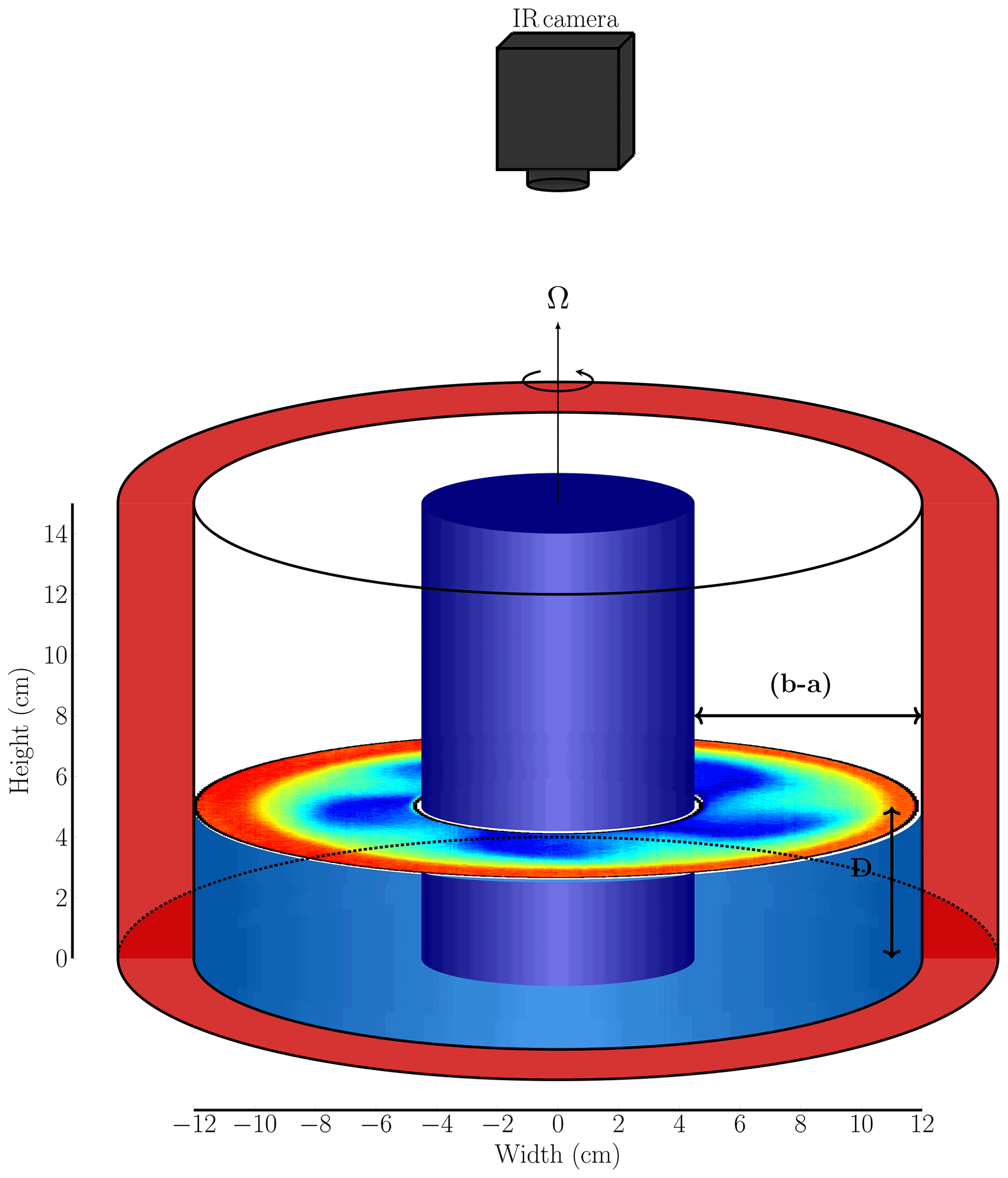
Figure 1 Schematic drawing of the experimental apparatus. The water in the inner cylinder (in blue) is cooled using a thermostat. Heating wires heat the water in the outer ring (in red). The water in the inner gap (b−a) is subjected to a radial differential temperature inferred by the insulating walls. The tank rotates anticlockwise at a constant rotation rate Ω. The surface temperature of the fluid in the gap is measured by an infrared camera aligned with the axis of rotation.

Our experimental data set consists of nine separate runs that differ in the temperature set at the boundaries. The temperatures are increased for each successive experiment in a way that reproduces a warming scenario similar to the Arctic amplification in the experiment; namely, the cold bath temperature is increased on average 1.75 times more than the temperature in the hot bath. In the rest of the paper, we use the more general term “polar warming” for this scenario. Sensors are placed in the outer warm and inner cold ring to measure the temperature in the two thermal baths, T_cold and T_warm, and calculate the radial temperature difference ΔT. Figure 2 and Table 1 show the mean temperature measured by these sensors as a function of the temperature set in the cooling basin of the thermostat for each experimental run. It can be seen in Fig. 2 that the mean temperature increases throughout the runs. More details about the technical setting of the two thermal baths are given in Appendix A.

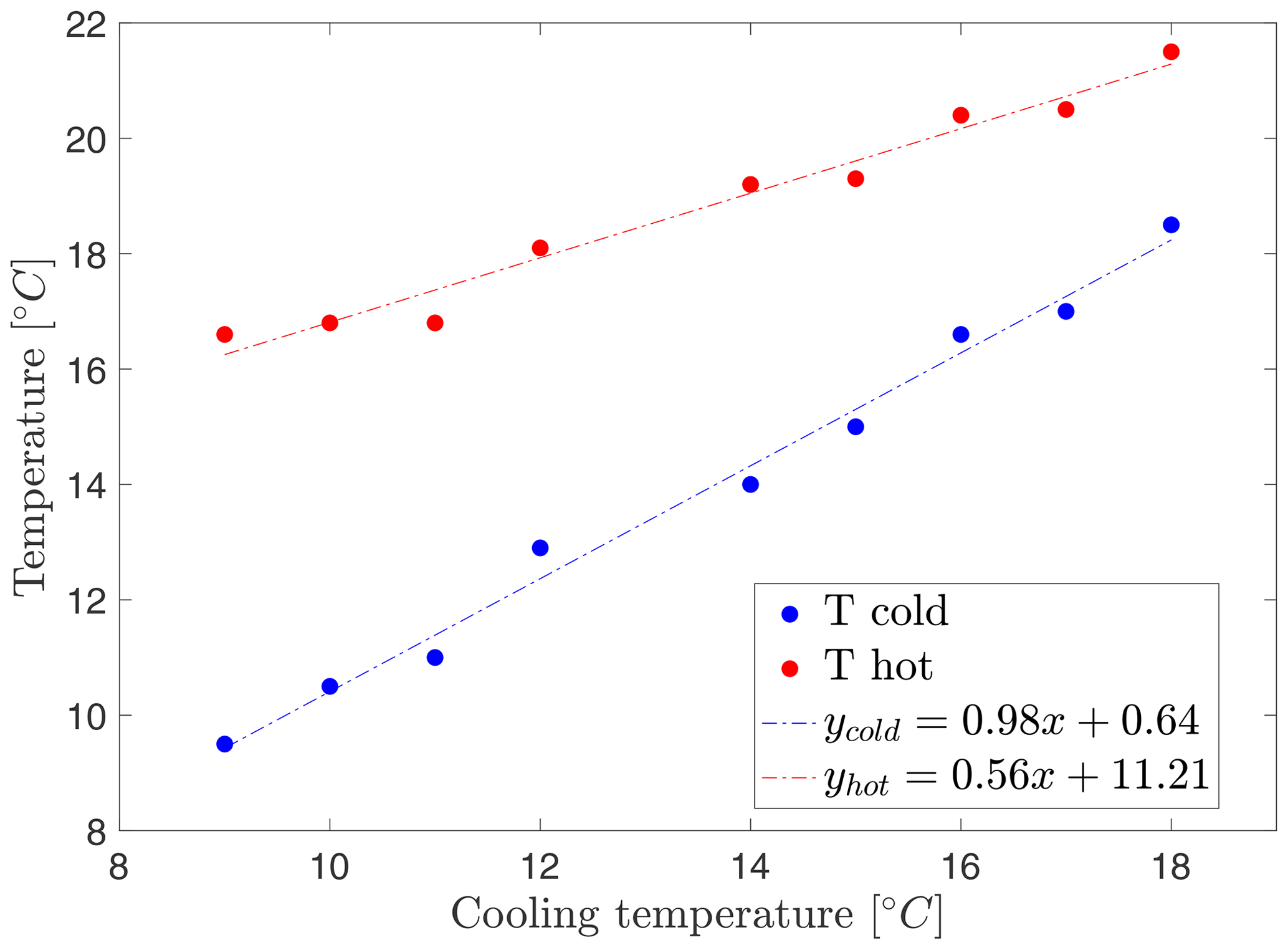
Figure 2 Temperature in the cold inner cylinder (blue) and hot outer ring (red) as a function of the cold thermostat target value. In the experiments discussed here (see Table 1), the temperature of the cooled water was increased 1.75 times more than the temperature of the heated water. The series of experiments form an Arctic amplification scenario with an increase in mean temperature but a decrease in the radial temperature gradient.

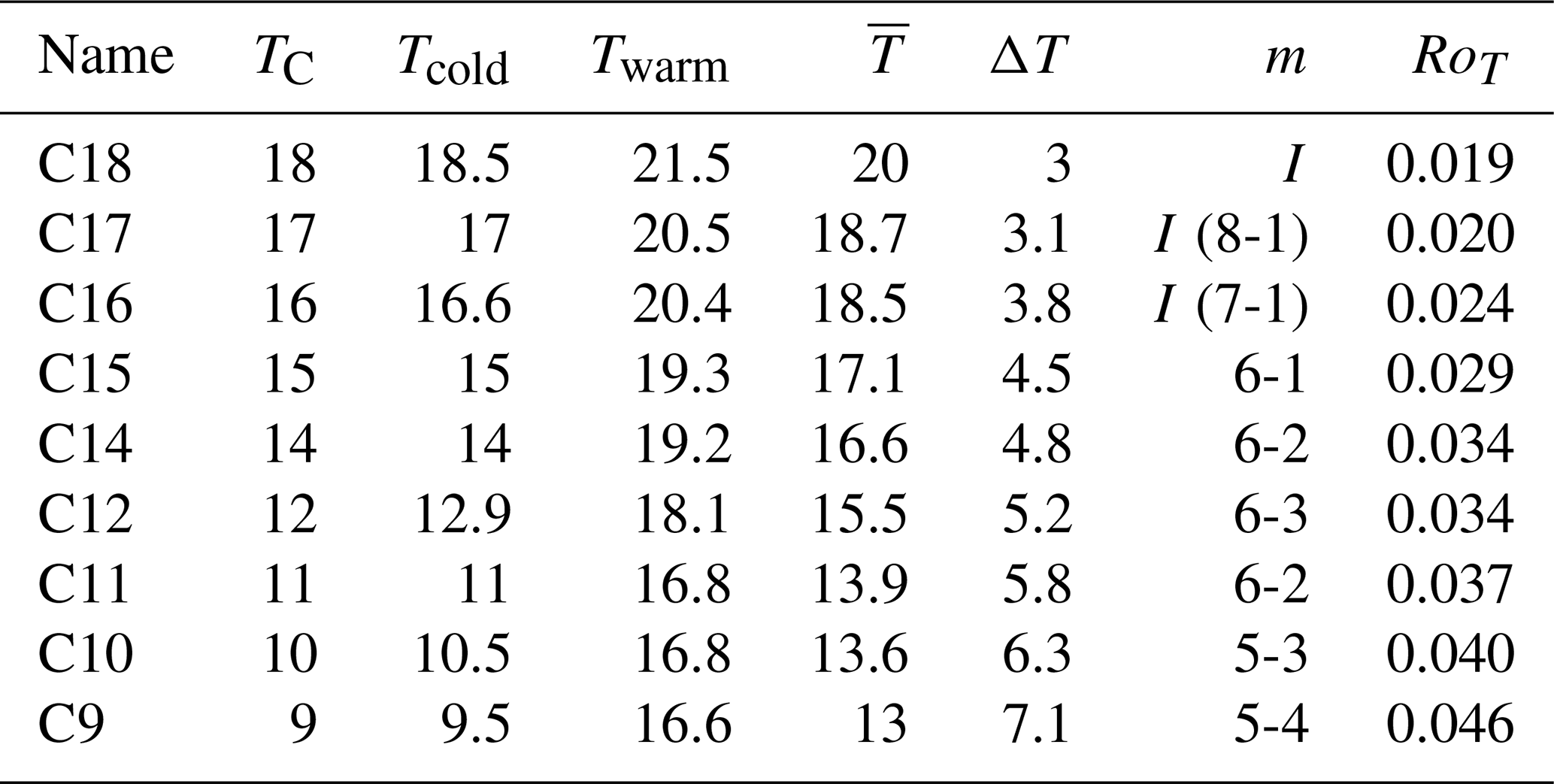
Table 1 Overview of the experimental runs. T_C is the temperature of the cooling thermostat. T_cold and T_warm are the measured temperatures in the inner and outer ring, respectively. $\stackrel{\mathrm{‾}}{T}=(T_{\mathrm{warm}}+T_{\mathrm{cold}})/\mathrm{2}$ is the mean temperature. $\mathrm{\Delta }T=T_{\mathrm{warm}}-T_{\mathrm{cold}}$ is the radial temperature difference. m is the azimuthal wavenumber of the baroclinic wave, and I indicates irregular waves. The rotation rate is Ω=8 rpm for all runs. Ro_T is the thermal Rossby number (Eq. 2). The Taylor number (Eq. 1) is $\mathit{Ta}=\mathrm{1.32}\times {\mathrm{10}}^{\mathrm{8}}$. All temperatures in the table are given in degrees Celsius.

After the experiment reaches thermal equilibrium, we start the rotation rate Ω set to 8 rpm anticlockwise. The centrifugal Froude number, defined as $\mathit{Fr}={\mathrm{\Omega }}^{\mathrm{2}}(b-a)/g$, where (b−a) is the gap width, is on the order of $\mathrm{5}\times {\mathrm{10}}^{-\mathrm{3}}$ and hence much smaller than 1. The system is allowed to run for the spin-up time (approximately 2 h), after which it reaches a stable state. Then, the data are collected for 7 h, corresponding to ca. 3000 revolutions of the tank. Given that each revolution corresponds to 1 terrestrial day, our experiment simulates nine cases with different pole-to-Equator temperature differences, each lasting for a little more than 8 years in the lab–Earth analogy.

The surface temperature is measured with an infrared camera, IR camera for short (Jenoptik camera module IR-TCM 640, with thermal sensitivity of 0.01 K and image resolution 640×480 pixels). The IR camera is fixed in the laboratory reference system and mounted at the top of the experiment (see Fig. 1). The IR camera outputs are the time series of the entire annulus 2D surface field measured once at each tank rotation, corresponding to a sampling interval dt=7.5 s. The advantage of having the 2D field is that some characteristics, such as dominant wave patterns, zonal phase speed (i.e. the speed at which the pattern drifts as a whole anticlockwise around the apparatus in the rotating frame), and changes in the structure, can be detected. The spatial and temporal resolutions are $\mathrm{400}\times \mathrm{400}\times \mathrm{3000}$ (pixels and times, $x,y,t$).

3 Flow regimes

This section discusses the dependency of the flow regimes on the radial temperature difference ΔT. Understanding how changes in ΔT impact the spatio-temporal flow features is a necessary first step for examining the effects on the temperature distribution.

Two nondimensional similarity parameters control the flow behaviour in a differentially heated rotating annulus (Hide and Mason, 1975): the Taylor number

$$\begin{array}{}\text{(1)}& \mathit{Ta}={\displaystyle \frac{f^{\mathrm{2}}(b-a{)}^{\mathrm{5}}}{{\mathit{\nu }}^{\mathrm{2}}D}}\end{array}$$

and the thermal Rossby number

$$\begin{array}{}\text{(2)}& {\mathit{Ro}}_T={\displaystyle \frac{gD\mathit{\alpha }\mathrm{\Delta }T}{f^{\mathrm{2}}(b-a{)}^{\mathrm{2}}}}.\end{array}$$

Here, g is gravity, f=2Ω the Coriolis parameter, Ω=8 rpm the tank rotation, $\mathit{\alpha }=\mathrm{0.207}\times {\mathrm{10}}^{-\mathrm{3}}$ K⁻¹ the volumetric thermal expansion coefficient, $\mathit{\nu }=\mathrm{1.004}\times {\mathrm{10}}^{-\mathrm{6}}$ m² s⁻¹ the kinematic viscosity of water, D=0.05 m the fluid depth, and $b-a=\mathrm{0.075}$ m the gap width. For relatively shallow fluid depths D, Rodda et al. (2020) found that the bottom Ekman layer has a significant impact on the dynamics of the flow and hinders the formation of baroclinic waves. For the experiments presented here, we chose a fluid depth such that the bottom drag is negligible.

A typical regime diagram can be drawn in the Ta–Ro space with the identification of flow regimes (Hide and Mason, 1975). Ro_T and Ta higher than the lower critical value define an anvil-shaped region where regular baroclinic waves develop in the fluid. Increases in Ta and decreases in Ro_T lead the flow towards a more irregular regime until it fully transitions to geostrophic turbulence, in which complex nonlinear wave interactions arise and the flow is irregular and non-periodic in time and space. Since we kept the tank rotation constant, the Taylor number, $\mathit{Ta}=\mathrm{1.32}\times {\mathrm{10}}^{\mathrm{8}}$, is constant as well, and Ro_T∼ΔT.

Table 1 lists the experimental runs and their parameters. T_C is the temperature of the cooling thermostat. T_cold and T_warm are the mean temperatures measured by sensors placed in the inner cold cylinder and warm outer ring, respectively, once a constant temperature difference ΔT is reached. Due to T_C rising, the mean temperature in the gap $\stackrel{\mathrm{‾}}{T}$ (resulting from a thermal equilibrium between the boundary walls) increases, even though the heating power supply to the outer ring is kept constant. T_cold and T_warm are plotted in Fig. 2 as a function of T_C. It can be noticed that T_cold (in blue) increases 1.75 times more than T_warm (in red in Fig. 2). This temperature change is well suited to experimentally mimicking the polar warming effect observed in the atmosphere.

3.1 Wavenumber transitions

It is enlightening to study the effects of lowering Ro_t on the flow regimes in the azimuthal wavenumber space. For our experiments $\mathit{Ta}=\mathrm{1.32}\times {\mathrm{10}}^{\mathrm{8}}$. Other experiments in similar setups have identified the threshold between regular baroclinic waves and geostrophic turbulence at Ta≈10⁸ (Harlander et al., 2011). Close to this transition, the flow becomes more complex due to the nonlinear interactions between the dominant mode and sidebands, resulting in mixed-mode states, and therefore the behaviour of the flow becomes less predictable (Früh and Read, 1997). Figure 3 displays surface temperature snapshots taken with the IR camera during different experimental runs and gives examples of flow regimes. Run C9 (Fig. 3a) is in a regular baroclinic-wave regime with a regularly shaped wave at wavenumber m=5. With smaller ΔT the complex interactions among waves result in wider spectra spanning several wavenumbers, as can be seen in Fig. 4, which shows the time evolution of the azimuthal wavenumber determined by calculating the spatial Fourier transform of the temperature data measured with a sampling rate of Δt=3.75 s along a constant radius r₀=0.063 m. In experiment C15 (Fig. 4a), the dominant wavenumber switches between m=3 and m=4 with sporadic transitions to higher and lower wavenumbers ranging between m=6 and m=1. This behaviour resembles that often referred to as structural vacillation in the baroclinic-wave literature (Hide and Mason, 1975). For decreasing Ro_T, it becomes more and more difficult to establish the dominant wavenumber associated with the flow as several transitions among other m values occur over time. In Table 1, we indicate the range of observed wavenumbers in the column marked by m. One can easily see that the range of wavenumbers broadens with decreasing ΔT. As it can be seen for experiment C18 (Fig. 4b), the flow is in a noticeably more irregular state, with a broad spectrum of excited wavenumbers. In the latter regime, it is challenging to identify a dominant azimuthal wavenumber m. We refer to this state as irregular (indicated by I in Table 1), where the flow has developed into geostrophic turbulence.

Figure 3 Flow regimes at ΔT=7.1 K (a), ΔT=5.2 K (b, c), and ΔT=3 K (d). The flow becomes more irregular for decreasing ΔT.

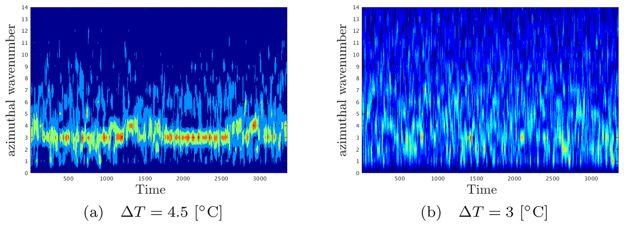
Figure 4 Azimuthal wavenumber evolution over time for experiments C15 (a) and C18 (b). The colour map represents the Fourier transform of temperature data sampled at a constant radius r₀=0.063 m. Larger ΔT values are associated with flows with a dominant wavenumber where sporadic transitions occur over time (a). When ΔT is decreased, the flow is irregular as a result of a superposition of wavenumbers (b).

3.2 Zonal phase speed

The zonal phase speed of the waves can be estimated by combining the thermal wind balance $U_T={\mathit{Ro}}_{T}fL/\mathrm{4}$ with Eq. (2):

$$\begin{array}{}\text{(3)}& U_T={\displaystyle \frac{g\mathit{\alpha }D\mathrm{\Delta }T}{f(b-a)}}.\end{array}$$

The linear theory by Eady (1949) predicts that the zonal phase speed of an unstable baroclinic wave in a zonal shear flow U=U₀z (U₀ constant) of depth D is $c=D{U}_{\mathrm{0}}/\mathrm{2}$. It follows that baroclinic Eady waves are non-dispersive, and each wave mode drifts with the same speed. Previous experimental studies (Fein, 1973; Vincze et al., 2015) have observed that the measured zonal phase speed as a function of $\mathit{\alpha }\mathrm{\Delta }T/f$ is better fitted by a more general power-law equation:

$$\begin{array}{}\text{(4)}& c=B(\mathit{\alpha }\mathrm{\Delta }T/f{)}^{\mathit{\zeta }},\end{array}$$

with $B=gD/(b-a)$ being a constant depending on the experimental configuration and the exponent ζ an empirical parameter. Note that for ζ=1, we obtain c=U_T given by Eq. (3). The Eady model can be used to make some quantitative predictions for the experimentally observed baroclinic waves, keeping in mind that the model is highly idealised and therefore some differences can be expected. The experiment has a free surface and bottom Ekman layer; therefore the zonal velocity, U, is not simply a linear function of z. Moreover, due to the lateral walls, the mean flow also shows a shear in the radial direction. Finally, rotation and the curvature of the sidewalls lead to slight free-surface deformation. These effects, taken together, introduce a weak dispersion into the baroclinic waves. Low-frequency vacillations might result from this dispersion even without nonlinear interactions, as discussed in detail by Harlander et al. (2011). Therefore, the zonal phase speed of the baroclinic wavefront, in our experiment taken as the contour line of the maximum velocity gradient along the radial direction, is challenging to predict, especially in regimes in which the dominant wavenumber changes over time (see Fig. 4).

In general, the zonal phase speed c_M can be defined as

$$\begin{array}{}\text{(5)}& c_M={\displaystyle \frac{\mathrm{1}}{m}}{\displaystyle \frac{\mathrm{d}\mathrm{\Phi }}{\mathrm{d}t}}={\displaystyle \frac{\mathrm{1}}{m}}\mathit{\omega }={\displaystyle \frac{\mathit{\lambda }}{T_{\mathrm{p}}}},\end{array}$$

where $\mathrm{\Phi }=\mathit{k}\mathit{x}-\mathit{\omega }t$ is the phase of a wave and $\mathit{\omega }=\mathrm{d}\mathit{\varphi }/\mathrm{d}t$, $\mathit{\lambda }=\mathrm{2}\mathit{\pi }/m$, and $T_{\mathrm{p}}=\mathrm{2}\mathit{\pi }/\mathit{\omega }$ are wave frequency, wavelength, and period, respectively. If we use the linear theory proposed by Eady, the waves can be assumed to be travelling with the same speed as the background flow, and therefore c_M≈U_T. To calculate c_M from the temperature data, we have extracted the temperature along a fixed radius R_d and plotted this as a function of time. In this way, we obtain a Hovmöller diagram with the azimuthal coordinate ϕ on the y axis and time on the x axis from which we can calculate the zonal phase speed graphically. The wavefronts appear in this plot as tilted lines of maximum temperature, and their slope is the zonal phase speed at which the baroclinic wave travels. We obtained the drift speeds by measuring the slope of 10 wavefronts and then calculating the mean value and the associated standard deviation. This procedure is repeated for each experimental run associated with a different ΔT.

The mean zonal phase speed c_M with the associated error is plotted in Fig. 5 as a function of $\mathit{\alpha }\mathrm{\Delta }T/f$. It is evident that decreasing ΔT slows down the zonal phase speed of the baroclinic waves. The dashed line in Fig. 5 depicts the general power-law equation (Eq. 4), where we calculated the coefficient ζ=0.55 by fitting the data. Figure 5 also shows that qualitatively the predictions from linear wave theory carry over to large-amplitude nonlinear waves. The zonal phase speed c predicted by Eq. (4) is close to the experimentally measured c_M, particularly for the regular flow regimes with a zonal wavenumber m=4 wave (the intermediate values of ΔT in runs C11–C15; see Table 1).

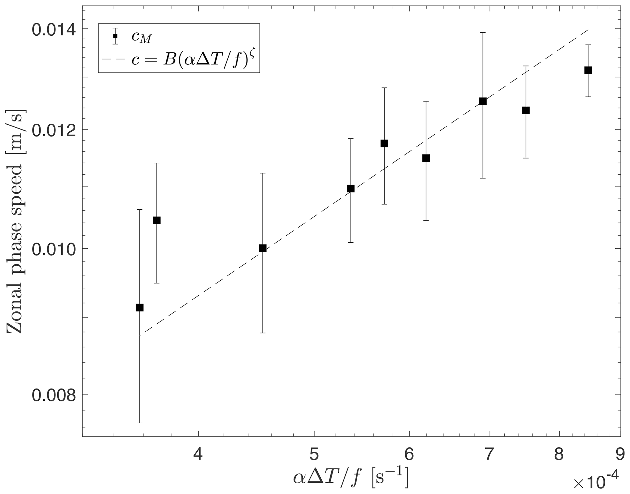
Figure 5 Log–log plot of the zonal phase speed c_M of the baroclinic wavefront for decreasing ΔT calculated from ϕ–t diagrams at a fixed radius R_d=0.087 m. The dashed line c is calculated from Eq. (4) with ζ=0.55.

Compared with Eady waves, dispersive Rossby waves are slower than the mean background flow for β>0. Note that a sloping topography can produce β<0, leading to faster propagation than the background flow. This holds in particular for long waves. Thus, from the zonal phase speed results, we can conclude that the effect of decreasing the radial temperature difference is to slow down the baroclinic wavefront. Hence, the propagation speed of extreme events embedded into the wave trains, e.g. in the form of exceptionally large meanders, will be slowed down, and the events in real atmospheric flows might unfold their local destructive potential over a more extended period.

4 Temperature distributions and variability

This section investigates how polar amplification affects temperature distributions, mainly focusing on the variability.

Figure 7 compares the probability density distributions of the temperature anomalies for all nine experimental runs. Temperature anomalies are calculated by subtracting the mean temperature from the measurements at each location “p”, “m”, and “e” (Fig. 6 shows their position in the annulus). Distributions at all three locations present a visible deviation from Gaussianity, which is more pronounced for larger ΔT. Noticeably, the polar and middle regions are characterised by broader temperature distributions, whilst the distribution in the outer region is much narrower. This difference tends to be less marked for smaller ΔT. For the polar and middle regions (left and middle plots), temperature variability consistently decreases for decreasing ΔT (red lines), with narrower and more symmetric distributions. In the subtropical regions, the tendency is the exact opposite: the distributions broaden for decreasing ΔT. The run “C9”, at the highest ΔT, stands out for its double-peaked distributions at all latitudes, which are also much broader than in all other runs.

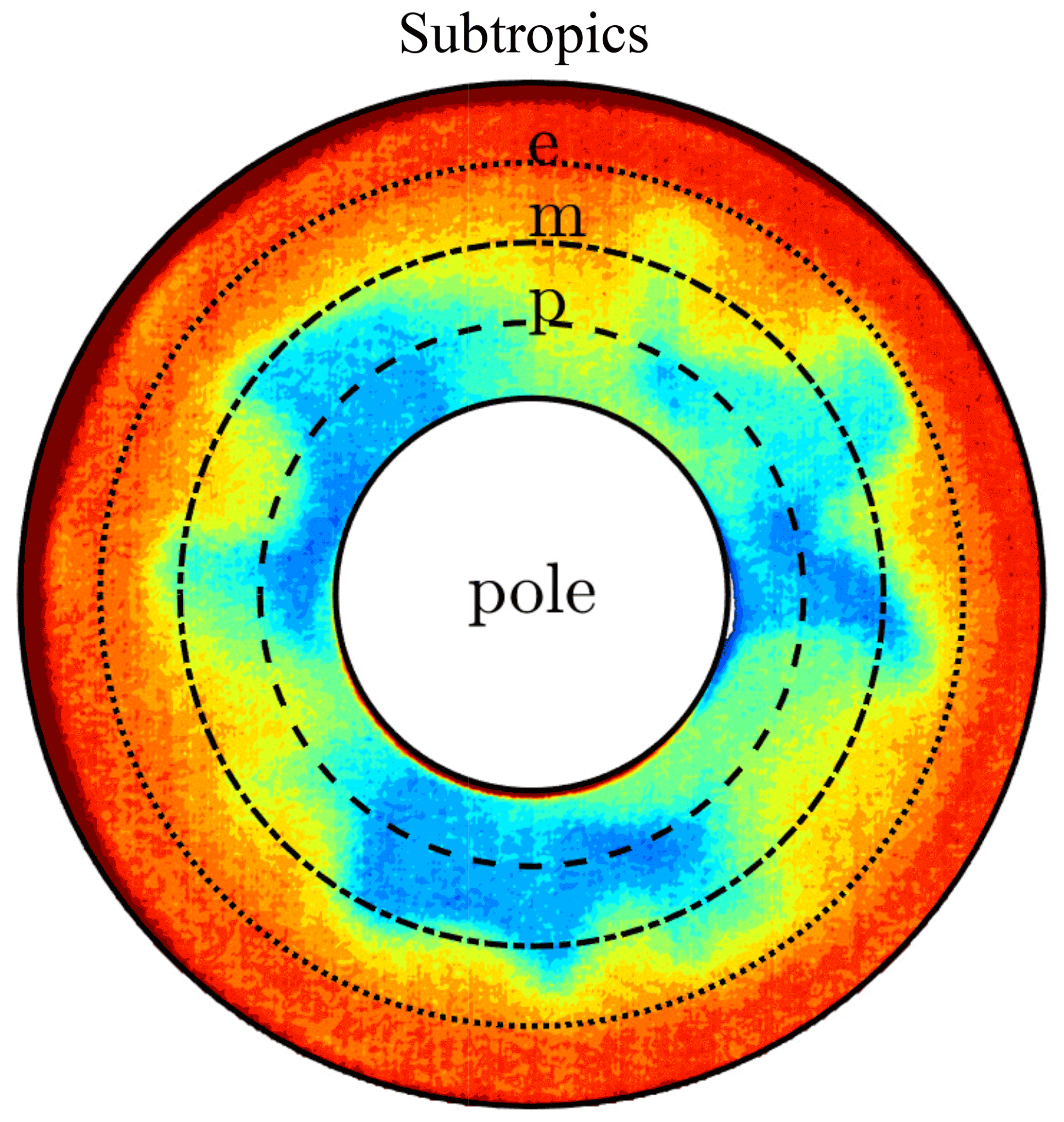
Figure 6 Three regions of the domain and location of the baroclinic wave: polar region (between the inner ring and the circle marked with p), mid-latitudes (between p and m), and subtropical regions (between e and the outer ring). The colours show the temperature measured for the experiment at ΔT=4.5.

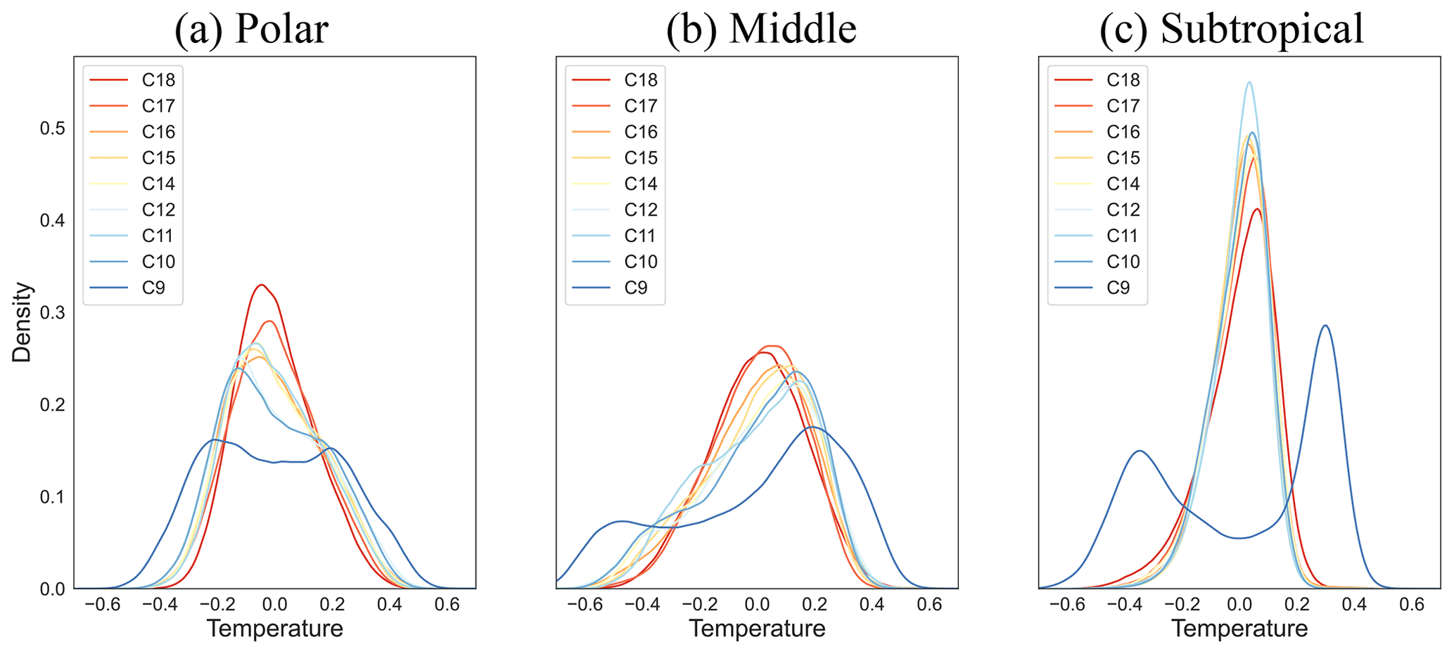
Figure 7 PDFs of temperature anomalies for the nine experimental runs at different ΔT values calculated at fixed latitudes p (a), m (b), and e (c); see Fig. 6 for the regions in the annulus.

The changes in temperature anomaly variability are quantified in Fig. 8, where standard deviation (left), skewness (middle), and excess of kurtosis (right) are plotted for the distributions at the three latitudes shown in Fig. 7.

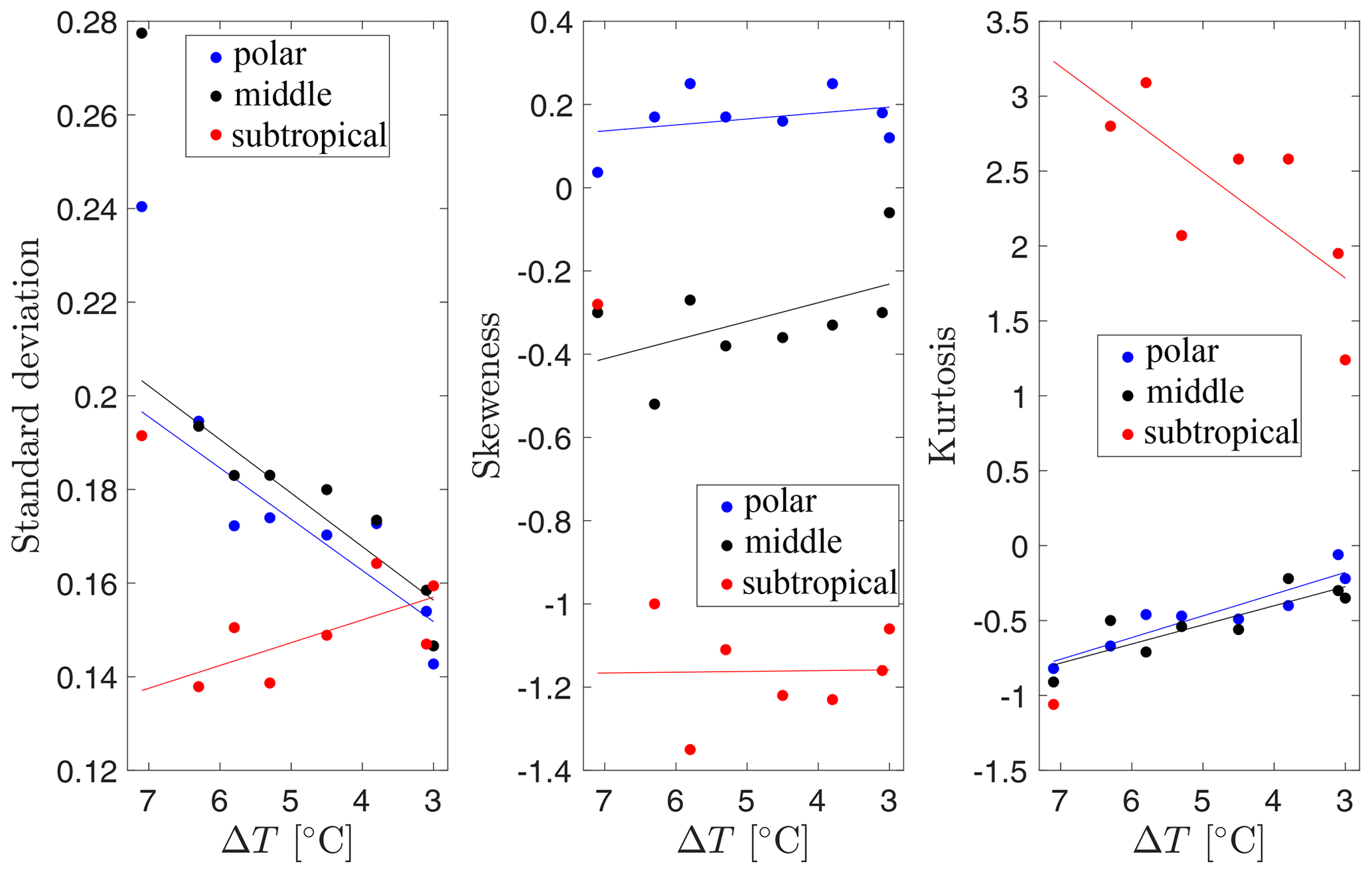
Figure 8 Standard deviation, skewness, and excess kurtosis trends for decreasing ΔT for the innermost ring (blue dots), the middle ring (black dots), and the outer ring (red dots).

The standard deviation decreases with decreasing ΔT in the polar and mid-latitude regions (blue and black lines), whilst it increases in the proximity of the subtropics (red line). To establish the statistical significance of the trends, we calculated the p value with the t test of the fit linear regression model fitlm, considering the 95 % significance level. Hence, we consider trends with p<0.05 as statistically significant, meaning that there is a probability higher than 95 % that the corresponding coefficient is different from zero.

The negative trends of the standard deviation are statistically significant (p=0.01 for the polar region, and p=0.003 for the middle region), but the positive trend in the subtropical region is nonsignificant (p=0.11). Note that the data point corresponding to the highest ΔT has been ignored to calculate the trends in Fig. 8 since it lies far off all the other data points. These points correspond to the double-peaked distributions in Fig. 7.

The excess kurtosis in Fig. 8 (right) shows an evolution towards more Gaussian distributions for decreasing ΔT, confirming what can be seen in Fig. 7. The polar and middle regions have a highly significant positive trend (p<0.001 in both cases). In the subtropical region, the excess kurtosis has a nonsignificant negative trend (p=0.5).

The skewness (Fig. 8 middle) is relatively robust under changes in ΔT: the polar data possess a right (positive) and the subtropical data a left (negative) skew without any significant trend. This opposite sign for the skewness is also observed in Garfinkel and Harnik (2017) in the case of measurements of near-surface tropospheric temperatures. Moreover, the skewness behaviour reminds us of the results by Belmonte and Libchaber (1996), who found for turbulent Rayleigh–Bénard convection that the temperature distribution skewness has a positive value at the cold (top) boundary and becomes more and more negative close to the warm (bottom) boundary. Belmonte and Libchaber (1996) attribute the observation of the negative skewness to the passing of a cold thermal front originating from the thermal boundary layer.

The skewness (Fig. 8 middle) does not show a statistically significant trend for any of the regions investigated. Linz et al. (2018) studied the effects of decreasing ΔT on temperature distributions in an idealised advection–diffusion model and concluded that whilst a smaller ΔT reduces the variance, it does not have any direct effect on the skewness and kurtosis. Changes in the kurtosis should be attributed to a response to changes in the flow field instead. Therefore, the lack of a clear trend in skewness in our data agrees with the results by Linz et al. (2018).

Our experimental data clearly show a relation between the decrease in meridional temperature difference and temperature variability. These results are consistent with what was found by Dai and Deng (2021) in model simulations and reanalysis data. Their analysis indicates that Arctic amplification decreases the temperature variability over the northern middle–high latitudes.

What does the reduction in temperature variability mean in terms of extreme events? Narrower and more symmetric probability distributions imply that cold and warm extreme events become weaker with decreasing ΔT. It follows that extreme events decrease in intensity in polar and middle regions, whilst near the subtropics, they become stronger. However, this does not help predict extreme events' duration or frequency. In the next section, we analyse the impact of changes in ΔT on the frequency of extreme events.

Extreme-event frequency

Extreme events are defined using a variety of metrics such as temperature thresholds and indices. The thresholds can be defined in different ways, the most common distinction being between relative thresholds (for example, defined by using specific percentiles of distribution or more straightforward measures like standard deviation) and absolute thresholds (for example, days with temperatures exceeding 35 ^∘C) (Seneviratne et al., 2021). Therefore, the choice of the definition used to calculate extreme events can affect the meaning of extremes and possibly the results.

We have discussed in Sect. 4 that the reduction in meridional temperature difference impacts the temperature variability and results in milder extreme temperatures from the poles to the mid-latitudes, whilst at low latitudes, the extremes might become stronger. To study whether this variability reduction impacts the frequency of extreme events, we define extreme temperature events based on a relative threshold. We chose such a threshold as the standard deviation (σ) calculated for each experimental run, corresponding to a fixed ΔT, on ensembles of data measured at fixed latitudes. We then call extreme cold/hot events all temperatures such that $|T-T_{\mathrm{mean}}|>\mathrm{2}\mathit{\sigma }$.

Note that the σ threshold is latitude-dependent. The extreme-event frequency is defined as the number of times the temperature crosses the set threshold normalised by the total length of the data set (which is, in any case, the same for all the data sets considered). The event duration is neglected; i.e. only the number of measurements (“days”) where the temperature exceeds the threshold is counted, without distinguishing whether such days are consecutive or isolated.

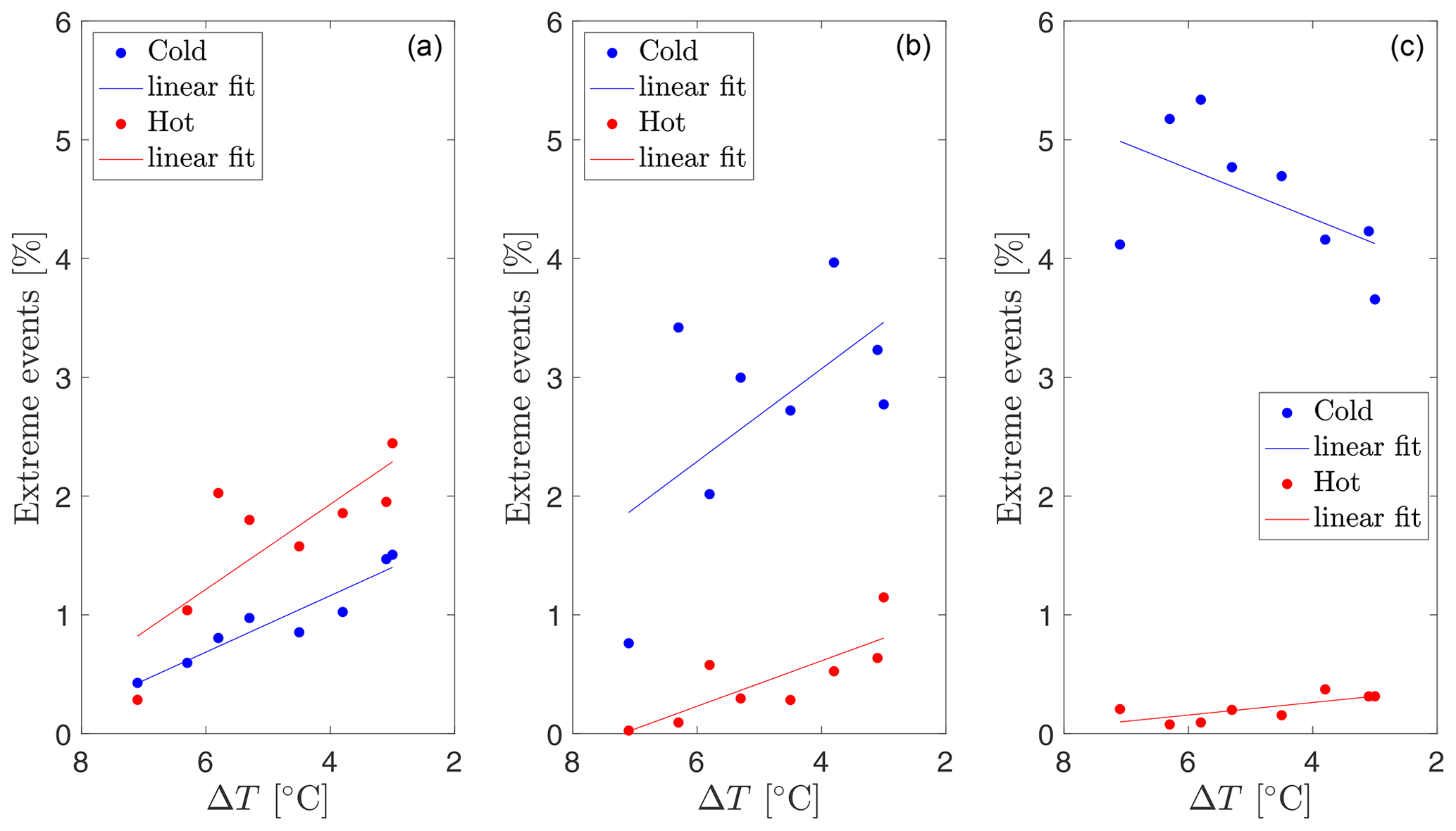
Figure 9 Trend of the cold (blue) and hot (red) extreme events with decreasing Equator–pole temperature difference. The trends are considered at three latitudes in the plot: polar latitude (a), mid-latitude (b), and subtropical latitude (c). The three latitudes are indicated in Fig. 10 by the labels p, m, and e, respectively.

The number of extreme events as a function of ΔT is plotted in Fig. 9 at the three locations p (in the left plot), m (in the middle plot), and e (in the right plot). The cold events are plotted in blue and the hot events in red. By comparing the three plots, one can immediately notice that the number of extreme cold and hot events is similar in the region near the pole (left plot). Still, the extreme cold events become increasingly frequent, moving towards the subtropics (middle and right plots). The second noticeable feature is that the hot extreme events show a statistically significant trend for all three regions (p=0.016 in the left plot, p=0.016 in the right plot, p=0.036 in the right plot in Fig. 9). This gives evidence for a hot extreme-event increment for decreasing ΔT. For the cold extremes, the left plot reveals a statistically significant positive trend (p<0.001) and the middle plot a positive trend as well, but it is statistically nonsignificant (p=0.055), whilst the right plot shows a statistically nonsignificant negative trend (p=0.08).

This difference in the cold trends can be partially explained by the fact that the baroclinic-wave dynamics do not govern the subtropical dynamics, and we have already suggested that the extreme-event distribution along the inner regions is tightly linked to the baroclinic waves. The decrease in cold events is consistent with a possible change in the subtropical extension of the baroclinic wave.

For a complete understanding, we also study how extreme events are distributed as a function of latitude. For this analysis, temperatures at fixed latitudes are collected into sets, where each set is constituted by 1.2×10⁶ temperature measurements for different times and longitudes. The standard deviation σ is calculated for each set, and, successively, the extreme-event frequency is calculated as a function of the latitude.

Figure 10 Number of extreme events (in percent) as a function of latitude in the experiment. Panel (a) depicts the cold events, whilst panel (b) depicts the hot events. The lines are solid for the experiment at ΔT=5.2 K, dashed at ΔT=3.8 K, and dotted at ΔT=3 K. The labels p, m, and e indicate the latitudes at which the trends shown in Fig. 9 are taken (see Fig. 6 to visualise their position).

The distributions are plotted in Fig. 10 for three experiments, namely at ΔT=5.2 K (solid line), ΔT=3.8 K (dashed line), and ΔT=3 K (dotted line). For easier visualisation, these three experiments have been chosen to represent the entire data set. The excluded data show similar results. The upper plot presents the extreme cold events, whilst we see the extreme hot events in the lower plot. Three latitudes labelled p, m, and e are indicated on the x axis for better readability.

For both plots, we notice that the three curves have similar shapes from the polar latitudes up almost to the point e, with more frequent extreme events for decreasing ΔT. Yet, the cold and hot extremes exhibit opposite trends: the cold-event frequency increases from the pole towards the subtropics with a maximum just before e and then decreases, whilst the extreme hot events behave in the opposite way. To some extent, the existence of a local maximum for warm and minimum for cold events at latitude e can be understood by looking at Fig. 6, where the latitude e (dotted line) marks the limit of the extension of the baroclinic-wave cold tongues, covering approximately three-quarters of the gap width. The external ring (between e and the subtropics in the figure) is unreached by the cold tongues; therefore, we can expect differences concerning extreme-event frequency in this part of the annulus where we find no baroclinic-wave activity. In this outer region, heat transport is mainly due to this meridional circulation, with some minor transport that might come from boundary layer instabilities and turbulent diffusion (von Larcher et al., 2018). The location of the maximum/minimum in cold-/warm-event frequency coincides with the utmost latitude to which the baroclinic waves extend. This clearly indicates that the baroclinic-wave activity shapes the frequency distribution.

In summary, we suggest that the large-scale baroclinic-wave dynamics govern the extreme-event spatial frequency distribution in the laboratory experiment.

5 High-variability events in NCEP data

After analysing the lab data for changes in variability and the distributions of high-variability events as a function of the north–south temperature gradient, it is instructive to see what atmospheric data show concerning changes in variability and variability extremes. We use the National Centers for Environmental Prediction (NCEP) reanalysis data (Kalnay et al., 1996). In contrast to operational counterparts, the reanalysis data do not suffer from inhomogeneities introduced by changes in the data assimilation system. In this respect, they are a good supplement to data based on individual instrumental records or climate-model simulations (Uppala et al., 2008). Moreover, reanalysis data cover historical data as well. We use two temperature data sets from the collection NOAA-CIRES 20th Century Reanalysis version 2 Daily Averages, covering the period from 1871 to 2012. The first set is the daily ensemble mean pressure level data (1000 to 10 hPa), from which we extracted just the 500 hPa level. The second set is the daily ensemble mean tropopause data. We start by considering the gradient and the standard deviation of the 500 hPa temperature from 1871 to 2012.

The upper panel of Fig. 11 shows the trend in the north–south temperature difference (ΔT) taken from the NCEP 500 hPa data for the Northern Hemisphere (blue line) and the Southern Hemisphere (red line). These temperature gradients are evaluated from the zonal mean temperature at 88^∘ N (88^∘ S) and the equatorial zonal mean temperature. We see that there is no significant change for the 500 hPa data in the Northern Hemisphere, except for a decline starting from the year 2000. In contrast, there is a long-term negative trend for the Southern Hemisphere. Despite some variability, the linear regressions (dashed lines) show a statistically significant trend towards more considerable north–south temperature differences for the Northern Hemisphere ($T\left(\mathrm{2012}\right)-T\left(\mathrm{1871}\right)=\mathrm{0.88}$ K, p=0.042) and smaller north–south temperature differences for the Southern Hemisphere ($T\left(\mathrm{2012}\right)-T\left(\mathrm{1871}\right)=-\mathrm{2.51}$ K, p=0.021). It is surprising at first glance that we do not see more clearly the warming of the Arctic (Arctic amplification) in the Northern Hemispheric data. However, the warming is pronounced particularly in surface data. For the lower stratosphere, the Arctic region is even cooled due to climate change (Stendel et al., 2021), and, as shown in the upper panel of Fig. 11, according to the NCEP data, even for the 500 hPa level, the warming is not obvious. This discrepancy between the change in the north–south temperature gradient for low and high levels of the troposphere drives the debate of whether climate change leads to more or less wavy jet streams (Stendel et al., 2021).

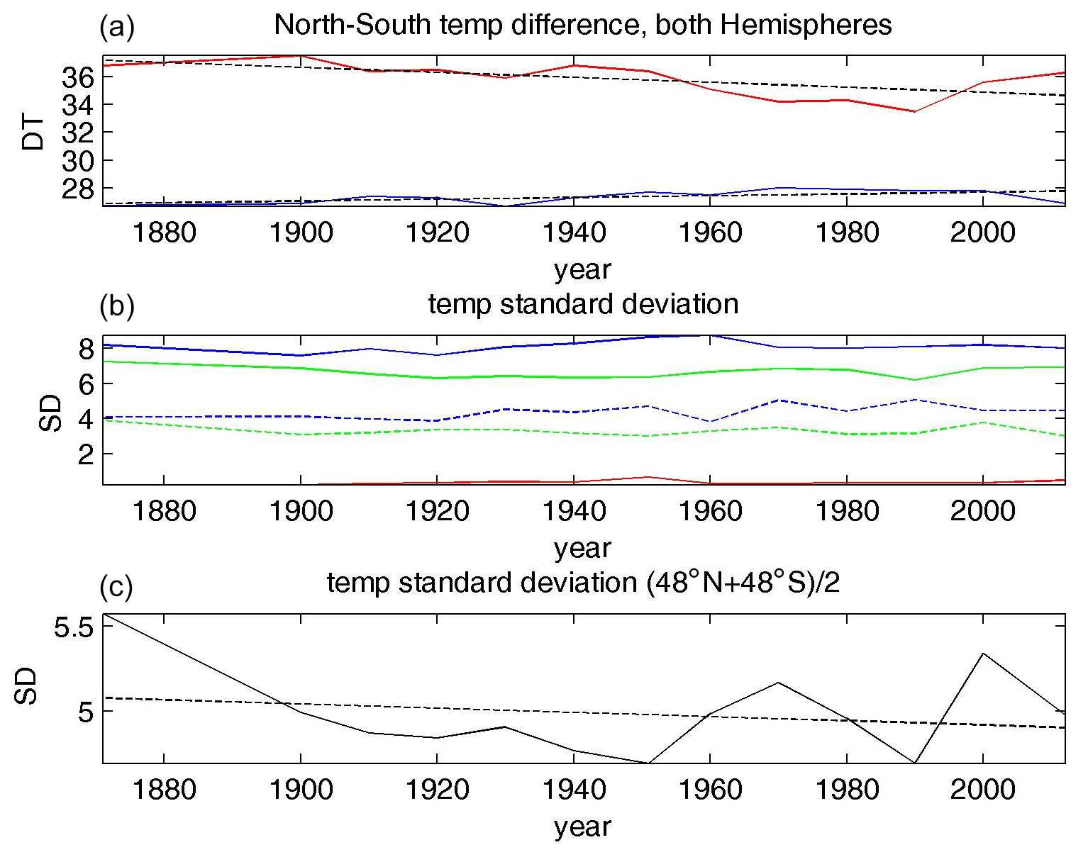
Figure 11 NCEP reanalysis data of 500 hPa temperature. (a) ΔT trend from 1871 to 2012, Northern Hemisphere (blue) and Southern Hemisphere (red). The linear regression (dashed line) shows a trend towards smaller north–south temperature differences in the Southern Hemisphere ($T\left(\mathrm{2012}\right)-T\left(\mathrm{1871}\right)=-\mathrm{2.51}$ K) but a slightly larger difference for the Northern Hemisphere ($T\left(\mathrm{2012}\right)-T\left(\mathrm{1871}\right)=\mathrm{0.88}$ K). (b) Zonal mean temperature standard deviations for 88^∘ N, 88^∘ S (solid blue, dashed blue), 48^∘ N, 48^∘ S (solid green, dashed green), and equatorial (red). (c) Mid-latitude zonal mean temperature standard deviation of ($\left(T\right(\mathrm{48}{}^{\circ }\mathrm{N})+T(\mathrm{48}{}^{\circ }\mathrm{S}\left)\right)/\mathrm{2}$) (solid line) and linear regression (dashed line). There is a weak trend towards decreasing standard deviation (${\mathit{\sigma }}_T\left(\mathrm{2012}\right)-{\mathit{\sigma }}_T\left(\mathrm{1871}\right)=-\mathrm{0.18}$ K).

The central panel displays the time evolution of the temporal standard deviation σ_T at different latitudes (solid blue, 88^∘ N; dashed blue, 88^∘ S; solid green, 48^∘ N; dashed green, 48^∘ S; red, Equator). The Northern Hemisphere exhibits a more significant variability, which might be related to a stronger land–sea contrast. For the mid-latitude time series, a small temporal decline can be seen (green lines), and the course of the curves looks very similar for both hemispheres. In the bottom panel, we highlight this trend by plotting just the mid-latitude zonal mean and the standard deviation of $\left(T\right(\mathrm{48}{}^{\circ }\mathrm{N})+T(\mathrm{48}{}^{\circ }\mathrm{S}\left)\right)/\mathrm{2}$ (solid line) and adding the linear regression (dashed line). Obviously, there is a weak but statistically not formally significant trend towards decreasing standard deviation (${\mathit{\sigma }}_T\left(\mathrm{2012}\right)-{\mathit{\sigma }}_T\left(\mathrm{1871}\right)=-\mathrm{0.18}$ K, p=0.49). Though not formally significant, this trend is consistent with other model data (Rind et al., 1989), and therefore it might still be physically significant. These observations are also in qualitative agreement with the results from the laboratory experiment.

To inspect the frequency of high-variability (extreme) events, we focused on NCEP reanalysis data of the tropopause temperature. These data are less prone to the effects of land–sea contrasts and might be closer to the lab experiment. Rodda and Harlander (2020) have shown that spectra from tropopause data are comparable to the frequency spectra of the baroclinic-wave experiment, and we suggest a similar connection concerning extreme values. We highlighted three 10-year periods: 1871 to 1880, 1951 to 1960, and 2003 to 2012. The seasonal cycle has been removed from the data. The frequency of extreme values, defined as values larger or smaller than twice the standard deviation, has been calculated for all longitude circles with an increment of 20^∘. Subsequently, for enhancing the robustness of the analysis, we took the mean of the Northern Hemisphere and Southern Hemisphere frequencies, and finally we zonally averaged the frequency data. This gives the mean frequency of extreme values as a function of latitude ranging from 90–0^∘.

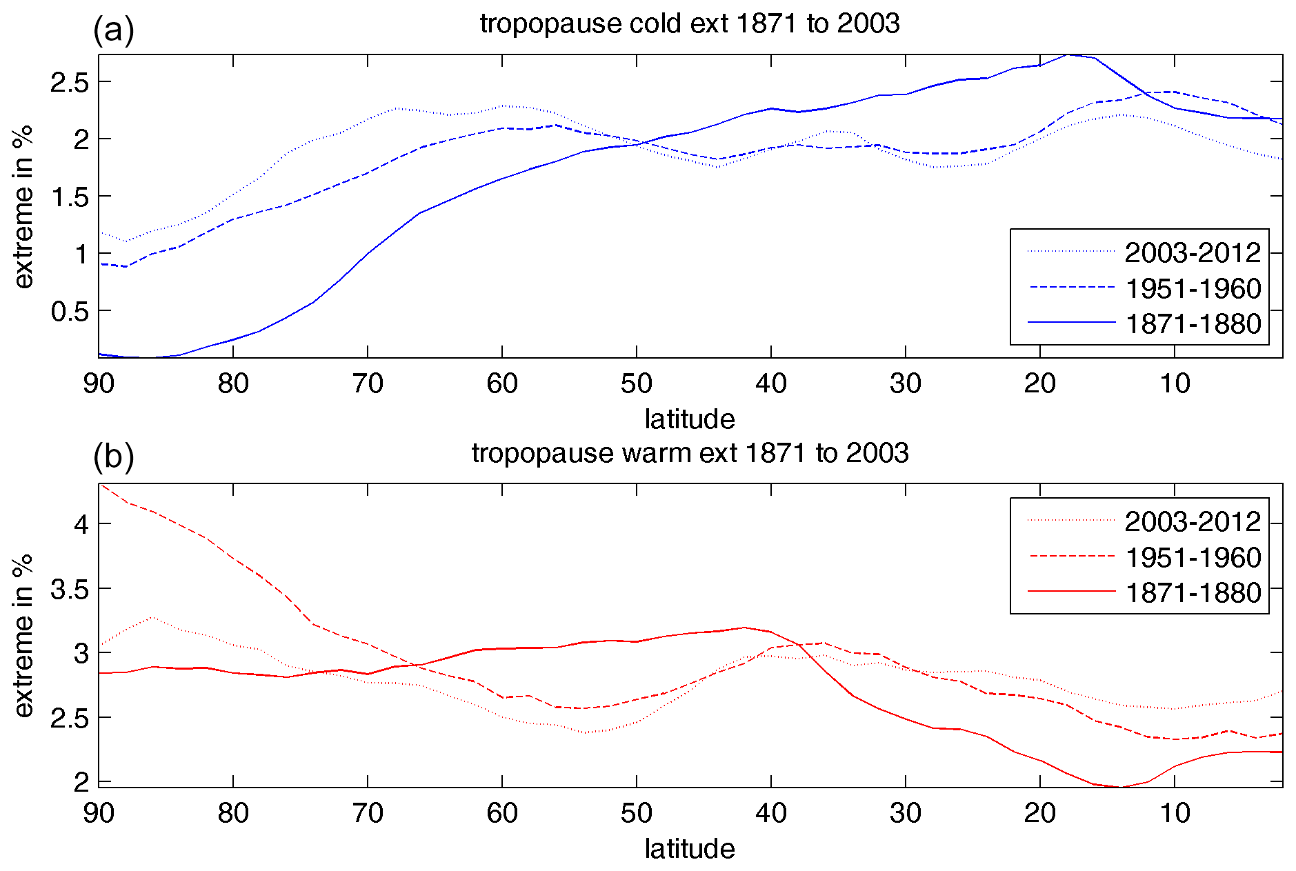
Figure 12 NCEP reanalysis data of tropopause temperature. Tropopause data have been chosen since the frequency spectra of the baroclinic-wave experiment look most similar to tropopause spectra (Rodda and Harlander, 2020). A number of extreme events in percent for different time slices and latitudes. The upper and bottom plots depict extreme cold and hot events, respectively. The lines are solid for 1871–1880, dashed for 1951–1960, and dotted for 2003–2012. The seasonal cycle has been removed from the data. The extreme values have been taken from the Pacific sector (weak land–sea contrast), and the frequencies from the Southern Hemisphere and Northern Hemisphere have been averaged for any latitudinal circle.

We see from Fig. 12 that the percentage of extremes, broken down to values above (warm, red curves) or below (cold, blue curves) the 2σ standard deviation threshold, ranges between 1 % and 4 %. For the cold case, the frequency of extreme events is larger at low latitudes, i.e. 1.7 % to 2.5 % in the latitude band from 30 to 10^∘ and 0.25 % to 2 % in the latitude band from 80 to 60^∘. We can see that the period 2003–2012, with the smallest north–south temperature gradient, shows the most extremes for polar latitudes (dotted blue line, 90 to 60^∘) but least for tropical latitudes (dotted blue line, 20 to 0^∘). Note that the experimental data lack a tropical dynamics (f plane with a wall as a southern boundary). Hence, one must be careful when comparing low-latitude NCEP data results with experimental data close to the heated outer sidewall. For the warm extremes, we see the highest frequency for the period 1951–1960 (dashed red line) near the polar region (more than 4 %). In this polar region, the most recent period shows more extreme warm events (dotted red line) than the historical data (solid red line) but about 1 % fewer than the period 2003–2012 (dashed red line). Obviously, for the frequency of extreme events, the strongest north–south gradient can be found for the decade 1951–1960 (dashed red line).

Comparing the experimental data (Fig. 10) with the NCEP data (Fig. 12), we find a notable qualitative similarity of the curves from p to e and from about 90 to 20^∘, respectively. Cold/warm extreme events occur more at low/high latitudes, in agreement with what was observed by Garfinkel and Harnik (2017). Furthermore, the cold events in NCEP and experimental data with large ΔT values are most numerous at low latitudes. The frequency decreases for lessening ΔT. In contrast, cold events are most probable for smaller ΔT for near-polar and equatorial latitudes. It should be noted that the NCEP data (Fig. 12) do not show such distinct extreme-event peaks around the near-Equator region but have a monotonic increase/decrease for cold/hot events instead. This difference can be expected since the appearance of a local peak in the experiment might be due to the mentioned missing tropical dynamics, as previously explained. Note further that the largest-ΔT experiment gives a very regular baroclinic wave (see Fig. 3a), which is somewhat unrealistic with respect to atmospheric flows. Caution is, therefore, required when comparing the ΔT=5.2 experiment with atmospheric temperature data.

6 Conclusions

We have presented a series of experiments with a differentially heated rotating annulus to model a global warming scenario. Our study aims to reproduce the Arctic warming and study the possible effects on other atmospheric phenomena. For this simple experimental environment, the impact of a reduced pole-to-Equator temperature difference on the mid-latitude large-scale dynamics and consequences for the likelihood and distribution of extreme events could be isolated from various processes that, in a more complex way, might also play a role in the Earth's atmosphere.

We found that the jet stream becomes more irregular due to warming at the pole, making it challenging to identify a clear dominant azimuthal wavenumber. Moreover, the eastward-propagating speed of the meandering baroclinic jet decreases, which, for the experiment, is a consequence of a slowdown of the westerly mean flow for reduced ΔT. The decreasing meridional temperature difference also leads to a reduction in the temperature variability in regions of the experiment where the baroclinic waves drive the dynamics. These regions, corresponding to polar and mid-latitudes, are characterised by temperature distributions that become narrower and more symmetric. Towards the outer ring of the annulus, corresponding to subtropical regions, the dynamics is less affected by the baroclinic, and consequently, the variability shows a slight increase. Our experimental findings agree with the recent analysis of coupled model simulations and ERA5 reanalysis by Dai and Deng (2021).

The consequence of a reduced temperature variability is that extreme events tend to become milder. However, our experiment also reveals that extreme cold/warm events tend to become more frequent. Furthermore, these events are larger in number at lower/higher latitudes independently of the time period and temperature differences considered in agreement with NCEP data and with measurements of near-surface tropospheric temperature reanalysis data (Garfinkel and Harnik, 2017).

We think the results of the study underpin the usefulness of the laboratory approach to understanding specific processes of climate change, in particular with a view to temperature variability and extreme events. However, we have only taken a first step and more sophisticated aspects like the use of extreme value theory, long-term memory effects, heavy tails in the amplitude of fluctuations, power laws, spatial correlations, and teleconnections have been neglected in the work presented here. Moreover, a more recent and bigger rotating tank has proven to be closer to the atmospheric case than the smaller system used here (Rodda et al., 2020). Hence, further experiments using this bigger differentially heated rotating tank and a deeper statistical analysis are planned for the future to add more experimental data to observations and climate simulations.

Appendix A: Heating and cooling in the experiment

In this Appendix, we give more details about how the heating and cooling devices of the experiment work and how the thermal equilibrium of the experiment is reached.

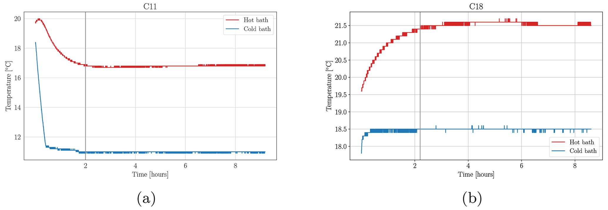
Figure A1 Time series of the temperatures measured in the outer (red) and inner (blue) rings for the experiments C11 (a) and C18 (b). The vertical grey line marks when the tank is set into rotation.

The water is circulated in the inner cylinder by pipes connecting it to an external device where the water is cooled to a set temperature and then pumped back. The temperature is, therefore, regulated by the thermostat. The outer ring hosts heating wires that heat the water. For all experimental runs, we kept the power supplied to the wires in the outer cylinder fixed and changed the temperature in the cooling thermostat. The system is then allowed to reach the thermal equilibrium before rotation is started. Figure A1 shows the time series of the temperature measured with sensors placed in the inner (in blue) and outer (in red) rings. It can be noticed that when rotation is started (vertical grey line), the temperatures in both baths have reached an equilibrium and remain stable for the entire duration of the experiment. From these considerations, we can conclude that the boundary conditions at the two conductive walls are of constant temperatures. Increasing the temperature in the inner cylinder increases the equilibrium temperature of the working fluid in the middle gap and, consequently, the equilibrium temperature for the hot bath (as can be seen in Fig. A1).