Quantifying stratospheric biases and identifying their potential sources in subseasonal forecast systems

The stratosphere can be a source of predictability for surface weather on timescales of several weeks to months. However, the potential predictive skill gained from stratospheric variability can be limited by biases in the representation of stratospheric processes and the coupling of the stratosphere with surface climate in forecast systems. This study provides a first systematic identification of model biases in the stratosphere across a wide range of subseasonal forecast systems.

It is found that many of the forecast systems considered exhibit warm global-mean temperature biases from the lower to middle stratosphere, too strong/cold wintertime polar vortices, and too cold extratropical upper-troposphere/lower-stratosphere regions. Furthermore, tropical stratospheric anomalies associated with the Quasi-Biennial Oscillation tend to decay toward each system's climatology with lead time. In the Northern Hemisphere (NH), most systems do not capture the seasonal cycle of extreme-vortex-event probabilities, with an underestimation of sudden stratospheric warming events and an overestimation of strong vortex events in January. In the Southern Hemisphere (SH), springtime interannual variability in the polar vortex is generally underestimated, but the timing of the final breakdown of the polar vortex often happens too early in many of the prediction systems.

These stratospheric biases tend to be considerably worse in systems with lower model lid heights. In both hemispheres, most systems with low-top atmospheric models also consistently underestimate the upward wave driving that affects the strength of the stratospheric polar vortex. We expect that the biases identified here will help guide model development for subseasonal-to-seasonal forecast systems and further our understanding of the role of the stratosphere in predictive skill in the troposphere.

1 Introduction

The Earth's stratosphere is home to several dynamical phenomena that are coupled with the tropospheric circulation. This coupling between the two layers can go in both directions; tropospheric variability drives variability in the stratosphere, but downward coupling from stratospheric variability can subsequently impact weather in the troposphere across the globe (Domeisen and Butler, 2020). As a result, the stratosphere is recognized as a source of predictability for the troposphere on subseasonal-to-seasonal (S2S) timescales (Butler et al., 2019a; Domeisen et al., 2020b). However, model simulations and forecasts often struggle to adequately capture such stratosphere–troposphere coupling processes. Model biases in both the troposphere and the stratosphere can impact these coupling processes, with potential deleterious effects for S2S predictability. The goal of this study is to provide a systematic identification of stratospheric biases in a wide range of S2S forecast systems.

In the wintertime extratropical stratosphere, variability in the upward flux of planetary-scale Rossby waves drives variability in the westerly circulation of the stratospheric polar vortices, affecting their midwinter strength and the timing of their seasonal breakdowns in spring (Andrews et al., 1987; Garfinkel et al., 2010). During winter and spring, anomalous behavior of the polar vortices can exert an influence on the underlying troposphere. This kind of “downward coupling” is especially apparent for extreme polar vortex events, including sudden stratospheric warming (SSW) events (Gerber et al., 2012; Baldwin et al., 2021), which are characterized by massive disruptions to the polar vortex that decelerate and reverse its westerly winds; strong vortex events, which are characterized by anomalous strengthening of the vortex (Limpasuvan et al., 2005; Tripathi et al., 2015); and final warmings, which denote the breakdown of the polar vortex in spring or early summer until the subsequent autumn (Black et al., 2006). The observed surface response following such polar vortex events generally resembles the so-called Northern Annular Mode and Southern Annular Mode (NAM and SAM; Thompson and Wallace, 2000; Baldwin and Dunkerton, 2001) or the North Atlantic Oscillation (NAO; Ambaum and Hoskins, 2002; Charlton-Perez et al., 2018; Domeisen, 2019), which captures the tropospheric response specifically over the North Atlantic, where Northern Hemisphere (NH) stratospheric influence tends to be the strongest (Butler et al., 2017; Dai and Hitchcock, 2021). The surface temperature and precipitation responses associated with these large-scale tropospheric circulation patterns have been shown to contribute to extreme events such as cold-air outbreaks and precipitation extremes (Domeisen and Butler, 2020).

In the tropical stratosphere, the absorption of vertically propagating tropical waves from the troposphere below drive the alternating phases of easterly and westerly winds of the Quasi-Biennial Oscillation (QBO; Baldwin et al., 2001). In turn, the QBO has the ability to modulate the tropospheric jet streams, tropical convection, and other phenomena such as the Madden–Julian Oscillation (e.g., Gray et al., 2018; Kim et al., 2020; Anstey et al., 2022, and references therein). These tropospheric teleconnections of the QBO are known to affect the NAO, as well as surface temperatures and precipitation near East Asia and in the tropics on both seasonal-mean and subseasonal timescales (Anstey et al., 2022; Gray et al., 2018; Haynes et al., 2021; Elsbury et al., 2021; Park et al., 2022). The QBO also has an apparent influence on the strength of the polar vortex, particularly in the Northern Hemisphere (NH), whereby easterly or westerly winds in the tropical lower stratosphere tend to lead to a weaker or stronger polar vortex, respectively (e.g., Holton and Tan, 1980; Calvo et al., 2007; Garfinkel et al., 2012; Anstey and Shepherd, 2014; Gray et al., 2018; Rao et al., 2020a). This is known as the “Holton–Tan” effect; there are several mechanisms that help explain such QBO–polar vortex coupling, but generally they are tied to the QBO winds affecting the propagation and dissipation of waves in the polar stratosphere.

Since the stratosphere and its variations generally exhibit a higher persistence and predictability than the troposphere (Domeisen et al., 2020a; Son et al., 2020), their downward influence can lead to opportunities for long-range prediction of surface weather on S2S timescales (Butler et al., 2019a). For example, all of the extreme polar vortex events mentioned above have shown potential for improved S2S surface prediction: SSWs (Sigmond et al., 2013), strong vortex events (Tripathi et al., 2015; Domeisen et al., 2020b), and final warmings (Butler et al., 2019b; Byrne et al., 2019). Tropical stratospheric variability associated with the QBO has also shown the potential to improve surface prediction on these timescales (Marshall and Scaife, 2009; Garfinkel et al., 2018; Martin et al., 2021b). However, surface prediction skill is not always improved based on the conditions in the stratosphere. In fact, several regions exhibit poorer predictability after extreme polar vortex events as compared to periods without them (Domeisen et al., 2020b). There are likely several reasons for these shortcomings in dynamical predictions related to the inherent chaotic nature of dynamical coupling within the atmosphere. For example, not all SSWs appear to have a significant downward impact (Karpechko et al., 2017), likely due to tropospheric internal variability (Domeisen et al., 2020c; Afargan-Gerstman and Domeisen, 2020) and the duration and strength of anomalies in the lower stratosphere following the SSW (Maycock and Hitchcock, 2015; Karpechko et al., 2017; Charlton-Perez et al., 2018; Domeisen, 2019; White et al., 2020).

Model biases and related shortcomings in simulating the stratosphere can affect dynamical predictions of stratospheric variability and stratosphere–troposphere coupling (Domeisen et al., 2020b; Charlton-Perez et al., 2013). Indeed, tropospheric biases identified independently of the stratosphere can sometimes be traced back to stratospheric anomalies in subseasonal forecasts; in the ECMWF extended-range prediction system, the persistence of the NAO was found to be constrained too strongly by the state of the polar vortex at initialization (Kolstad et al., 2020). Since stratospheric variability and extreme events are primarily governed by wave–mean flow interactions, biases in wave driving due to either resolved or parameterized processes can lead to biases in the mean state of the stratosphere, which can further alter its response to subsequent forcing (McLandress et al., 2012; Richter et al., 2014) and limit stratospheric predictability (Portal et al., 2022). More fundamentally, a model's vertical resolution in the stratosphere can influence its ability to realistically represent the stratosphere. For example, climate models with limited resolution in the stratosphere tend to dramatically underestimate stratospheric variability (Charlton-Perez et al., 2013; Shaw et al., 2014; Richter et al., 2020; Rao et al., 2020a). Similarly, subseasonal forecast systems with severely limited model resolution in the stratosphere exhibit poor skill in predicting extreme polar vortex events beyond 1 week, whereas systems with higher model lids and higher vertical resolution in the stratosphere can predict these events up to 2–3 weeks in advance (Domeisen et al., 2020a). Subseasonal forecast systems that poorly represent tropospheric stationary waves also tend to have low vertical resolution in the stratosphere, connected to larger stratospheric biases (Schwartz et al., 2022). On seasonal timescales, surface prediction skill can also in part be traced back to model properties such as vertical resolution in the stratosphere (Butler et al., 2016; Portal et al., 2022).

It is expected that identifying and properly addressing the sources of stratospheric biases would not only improve prediction in the stratosphere but also help improve the surface prediction skill associated with the aforementioned stratospheric phenomena. For example, some recent studies have investigated the impact of explicitly correcting stratospheric biases in model simulations and found improvements to SSW statistics (Tyrrell et al., 2021) and the representation of the Holton–Tan effect (Karpechko et al., 2021). In other similar studies, teleconnections to the polar vortex related to Siberian snow cover (Tyrrell et al., 2020) and the El Niño–Southern Oscillation (ENSO; Tyrrell and Karpechko, 2021) were shown to be sensitive to model stratospheric biases. In the case of the Siberian snow cover, explicitly correcting the stratospheric biases had modest impacts on the magnitude and duration of downward coupling between the polar vortex and the NAM/NAO. However, in the case of ENSO teleconnections, correcting stratospheric biases had no detectable impact on the NAO, possibly because the NAO response to the strong ENSO events in the experiments was dominated by the tropospheric ENSO pathway to the North Atlantic (Jiménez-Esteve and Domeisen, 2018).

Given the role the stratosphere can play in skillfully predicting surface weather at subseasonal-to-seasonal timescales, it is crucial to investigate and diagnose the stratosphere and stratosphere–troposphere coupling biases present in such models. Identifying and comparing these biases will serve as a data point for improving subseasonal forecast systems and ultimately prediction skill, both in the stratosphere and for extended-range surface weather. Herein we perform a comprehensive investigation and intercomparison of stratosphere-related biases affecting subseasonal prediction systems. The present work is the result of a volunteer collaborative effort of the World Climate Research Programme (WCRP) Stratosphere-troposphere Processes And their Role in Climate (SPARC) Stratospheric Network for the Assessment of Predictability (SNAP) activity, which is also the stratosphere sub-project of the WCRP–World Weather Research Programme S2S Prediction Project. In Sect. 2 we describe the datasets and methods we use to identify biases. We describe our results in Sect. 3 and discuss and summarize our findings in Sect. 4.

2 Data and methods

2.1 Subseasonal-to-seasonal (S2S) hindcast and reanalysis datasets

We primarily use ensemble hindcast data from the S2S Prediction Project Database (Vitart et al., 2017). Where possible, we also include results from other ensemble forecast systems that do not provide data to the S2S database; these include the National Oceanic and Atmospheric Administration's Global Ensemble Forecast System version 12 (NOAA GEFSv12; Hamill et al., 2022; Guan et al., 2022), the Geophysical Fluid Dynamics Laboratory Seamless System for Prediction and EArth System Research (GFDL-SPEAR; Delworth et al., 2020), the National Center for Atmospheric Research Community Earth System Model version 2 (CESM2) with version 6 of the Community Atmosphere Model as its atmospheric component (NCAR CESM2-CAM6, hereafter CESM2-CAM or CESM2-C), and CESM2 with the version-6 Whole Atmosphere Community Climate Model as its atmospheric component (CESM2-WACCM6, hereafter CESM2-WACCM or CESM2-W; Richter et al., 2022).

Table 1 lists the different S2S forecast systems and includes relevant information about their hindcast and model configurations. Because the hindcast periods available for different systems vary substantially, unless noted otherwise, we limit our analyses to the 1999–2010 period, which is common to nearly all systems. The one exception is GEFSv12, which has hindcasts that span the period from 2000–2019, for which we simply use the 2000–2010 period. In order to balance including as many prediction systems as possible with also being inclusive of contributions from co-authors with differing capabilities to access and store the large datasets involved, we designated the S2S database systems that provide at least 35 d forecasts as our “core systems” while others were considered optional. Thus, the number of S2S systems shown for a given analysis may vary but will always include the seven core systems from the S2S database.

Table 1 Details of the subseasonal-to-seasonal forecast systems used herein.

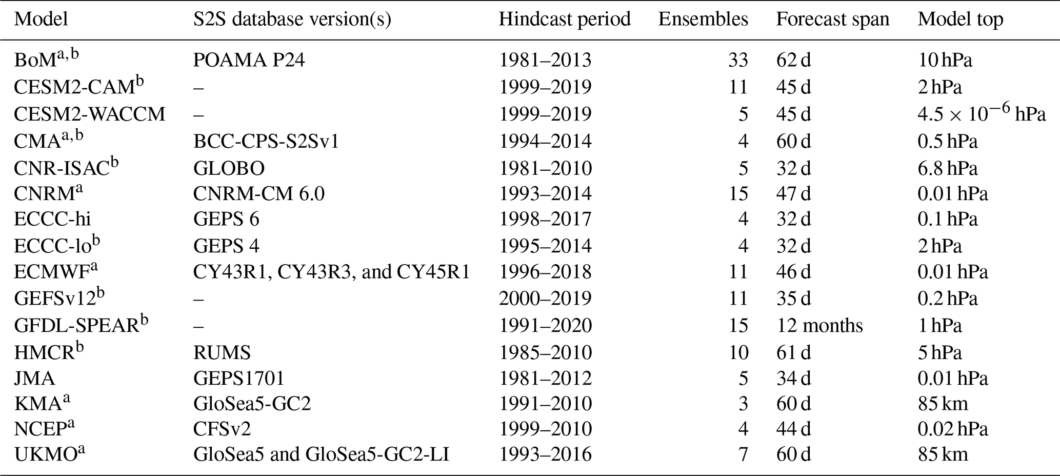
CESM2-WACCM hindcast initializations were only performed for September–April. HMCR is not considered a core system since there are no data available for 10 hPa. ^a Core systems. ^b Systems with low-top models.

There are often multiple model versions of hindcast data available within the S2S database, representing updates to the forecast systems. These model updates sometimes include changes that can reasonably be expected to affect behavior in the stratosphere, such as increases in the number of model levels or lid height or changes to the atmospheric initialization. Table 1 lists the specific model versions we use; the important ones to note are for the CMA, ECMWF, and ECCC systems. In order to cover the 1999–2010 hindcast period, for ECMWF we consider only CY43R1, CY43R3, and CY45R1 to prevent mixing cycles with large changes to the prediction systems; cycles beyond CY46R1 were excluded because these hindcasts were initialized with ERA5 reanalysis, include updates that explicitly affect mean stratospheric biases (Polichtchouk et al., 2020), and do not fully cover the 1999–2010 period. The CMA and ECCC data both have model versions available in the S2S database that include changes to significantly higher model tops. Since we consider CMA to be a core system (as it performs forecasts beyond 35 d), we use the older low-top version known as “BCC-CPS-S2Sv1” because the more recent “BCC-CPS-S2Sv2” hindcast period only covers 2004–2018. In contrast, ECCC data are considered to be optional, so some analyses use either the high- or the low-top versions; in such cases, we explicitly describe these as “ECCC-hi” or “ECCC-lo”, respectively (see Sect. 2.2 for the specific definitions of high versus low top).

For the analyses herein, we use basic meteorological fields, including zonal and meridional wind components, temperatures, and geopotential heights. These fields from the S2S database are provided once daily at instantaneous 00:00 UT verification times on a $\mathrm{1.5}{}^{\circ }\times \mathrm{1.5}{}^{\circ }$ latitude × longitude grid, with 10 pressure levels between 1000 and 10 hPa (with about 3 levels in the stratosphere, including 100, 50, and 10 hPa). GEFSv12 fields are provided 6-hourly on a $\mathrm{0.5}{}^{\circ }\times \mathrm{0.5}{}^{\circ }$ grid, with 25 pressure levels between 1000 and 1 hPa (6 between 100 and 10 hPa). GFDL-SPEAR fields are also 6-hourly on a $\mathrm{0.5}{}^{\circ }\times \mathrm{0.5}{}^{\circ }$ grid, with 33 pressure levels between 1000 and 1 hPa. For the CESM2-CAM and CESM2-WACCM data, we make use of the available “zonal-mean” collection of variables that are provided as daily means on pressure levels closest to the model levels; we interpolate these data to a set of 32 standard pressure levels between 1000 and 10 hPa (with 6 between 100 and 10 hPa); these fields have 192 latitudes (∼0.9424^∘ resolution) from the finite-volume grid.

The subseasonal hindcast datasets used are all initialized with different atmospheric analyses. Therefore, to ensure that comparisons and biases are all determined with respect to a consistent dataset, we compare hindcast fields to those from the ERA-Interim (ERA-I) reanalysis (Dee et al., 2011). Different modern reanalysis products generally agree very well among one another for the time periods (post-1999) and levels (10 hPa and below) we consider (Long et al., 2017; Gerber and Martineau, 2018; Fujiwara et al., 2021), and thus our results are unlikely to be sensitive to the choice of reanalysis.

2.2 Methods

Throughout the paper we distinguish between forecast systems with low- and high-top atmospheric models. We define the systems having model tops at or above 0.1 hPa with several levels above 1 hPa as high-top; any others that do not meet these criteria are specified as low-top. In total, we consider eight systems with high-top models and eight systems with low-top models (see Table 1); however, the precise number of models included in a given analysis varies. In our figures, we highlight low-top models with asterisks and/or dashed lines.

For a given diagnostic, raw biases among the forecast systems are computed by taking the difference between the ensemble-mean hindcasts and ERA-I. We generally composite these biases according to lead time and/or season in order to determine the systematic differences in the hindcast predictions from reanalysis. For some applications we derive lead-time-dependent climatologies for the different forecast systems, which we use to determine forecast anomalies and to apply bias correction. For systems in the S2S database, these climatologies are found by averaging all ensemble-mean hindcasts for a given day of year at a specific lead time. For systems that provide a fixed set of hindcast initializations that do not uniformly cover the same days of year in the hindcasts (such as the GEFSv12 and the CESM2 systems), we create the lead-dependent climatologies according to the method outlined in Pegion et al. (2019); briefly, this method involves averaging all hindcasts for a given day of year and lead time (which is generally less than the total number of years in the hindcast archive) and then applying a rolling 31 d average with centered triangular weights to the “raw” and noisy lead-dependent climatology. Hindcast anomalies are then determined by subtracting these climatologies for a given day of year and lead time from the raw forecast quantities. In some cases we apply a linear bias correction to raw quantities in order to remove any climatological drift that may exist. This is done by removing the difference between each system's lead-time-dependent climatology and the ERA-I climatology from the predicted quantity in question: $Q_{\text{BC}}(t,l)=Q_{\text{Raw}}(t,l)-\left[{\stackrel{\mathrm{‾}}{Q}}_{\text{hc}}\right(t_{\text{doy}},l)-{\stackrel{\mathrm{‾}}{Q}}_{\text{obs}}(t_{\text{doy}}+l\left)\right]$, where Q_BC is the bias-corrected quantity, Q_Raw is the raw quantity, ${\stackrel{\mathrm{‾}}{Q}}_{\text{hc}}$ is the hindcast climatology, ${\stackrel{\mathrm{‾}}{Q}}_{\text{obs}}$ is the observed/reanalysis climatology, t is the forecast initialization date, l is the lead time, and t_doy is the day of year of the initialization date t.

In Sect. 3.3 we investigate whether there are biases in relation to extreme stratospheric events, including SSWs and strong vortex events in the NH. SSWs are defined using ERA-I data, based on reversals in the 10 hPa 60^∘ N zonal-mean zonal winds, consistent with Charlton and Polvani (2007) and Butler et al. (2017). Similarly to SSWs, strong vortex events are defined using ERA-I data when the daily mean 10 hPa 60^∘ N zonal-mean zonal winds exceed 41.2 m s⁻¹ for at least 2 consecutive days, corresponding to the 80th percentile of the November–March 1980–2012 zonal winds, consistent with the definition used by Tripathi et al. (2015). These definitions have also been employed in prior investigations of the stratosphere in S2S systems (Domeisen et al., 2020a, b). The central dates of these events are considered to be the first day on which these zonal-wind thresholds are met.

3 Results

3.1 Global- and zonal-mean biases

From the perspective of model evaluation, examining mean state biases in the stratosphere is useful since the processes that govern the distribution of zonal-mean temperatures and winds in the stratosphere are quite well understood. Global- and annual-mean temperatures in the stratosphere should be very close to radiative equilibrium (e.g., Olaguer et al., 1992). In contrast, seasonal and meridional variations in zonal-mean stratospheric temperatures and winds arise from dynamic influences such as wave–mean flow interaction. Meridional circulations driven by the dissipation of waves drive stratospheric temperatures away from radiative equilibrium, which affects the zonal-mean zonal winds through thermal-wind balance (e.g., Andrews et al., 1987; Shepherd, 2000). Model biases in global annual-mean stratospheric temperatures and/or seasonally varying biases in zonal-mean temperatures and winds therefore provide information about the likely origin of model errors, pointing to either model components that affect radiative processes or those that affect middle atmosphere dynamical processes such as parameterized gravity wave drag.

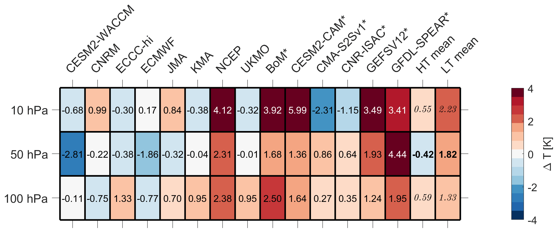
Figure 1 Global- and annual-mean temperature biases at a lead time of 4 weeks. The columns show individual forecast systems, while the rows correspond to different pressure levels. The numerical values displayed are shown in kelvins (K). Asterisks at the end of names denote the systems with low-top models. The last two columns show the high-top (HT) and low-top (LT) composites; the bolded/italicized text in these boxes denotes composite differences that are/are not significant at the 95 % level from Student's t test.

We first consider the annual, global-mean temperature biases among the S2S forecast systems. Figure 1 shows these biases for 10, 50, and 100 hPa for each of the models at a lead time of 4 weeks (days 22–28). These biases generally develop and increase in magnitude monotonically with lead time, with many of these biases being present at earlier lead times of 1–2 weeks (not shown). The magnitude of biases tends to be largest in the middle stratosphere at 10 hPa, with six of the models shown exceeding absolute biases over 2 K. Positive temperature biases tend to be most common across the models and levels, with the exception of ECMWF and CESM2-WACCM, which primarily have negative temperature biases.

There are some apparent differences between the annual, global-mean stratospheric temperature biases between the systems with high- and low-top models (denoted with asterisks). Warm biases are more common across the pressure levels in the low-top systems, and the highest-magnitude biases are generally at 10 hPa, which is likely related to the model tops being relatively close to this level. Some of the low-top systems (CMA-S2Sv1 and CNR-ISAC) have biases that are much less severe in the lower stratosphere and more comparable to the high-top systems. The biases for the high-top systems are generally smaller in magnitude, but there are some exceptions: for instance, the CESM2-WACCM, ECMWF, and NCEP systems have biases at some levels that are as large as or larger in magnitude than the low-top systems. Annual-mean, global-mean temperature differences between the high- and low-top composites are thus only significant at 50 hPa (numbers in bold), where the low-top systems have only positive biases and the high-top systems have mostly slight negative biases. However, it is still worth noting that at 10 hPa the magnitude of the low-top biases all exceed 1 K, while all high-top systems except for NCEP are below 1 K.

Figure 1 also highlights some “familial” relationships. In particular, the “NOAA family” of forecast systems (including GEFSv12, GFDL-SPEAR, and NCEP) all show global-mean warm biases throughout the lower and middle stratosphere. The biases in the KMA and UKMO systems are very similar, likely owing to the fact they both use the same GloSea-5 model (see Table 1). There are large differences between the biases apparent in CESM2-CAM and CESM2-WACCM, which may be due to a combination of factors: aside from the differences in model tops, CESM2-WACCM includes fully interactive tropospheric and stratospheric chemistry (Gettelman et al., 2019; Richter et al., 2022), and the atmospheric models are initialized with different reanalyses (“CFSv2” for CESM2-CAM and “MERRA-2” for CESM2-WACCM).

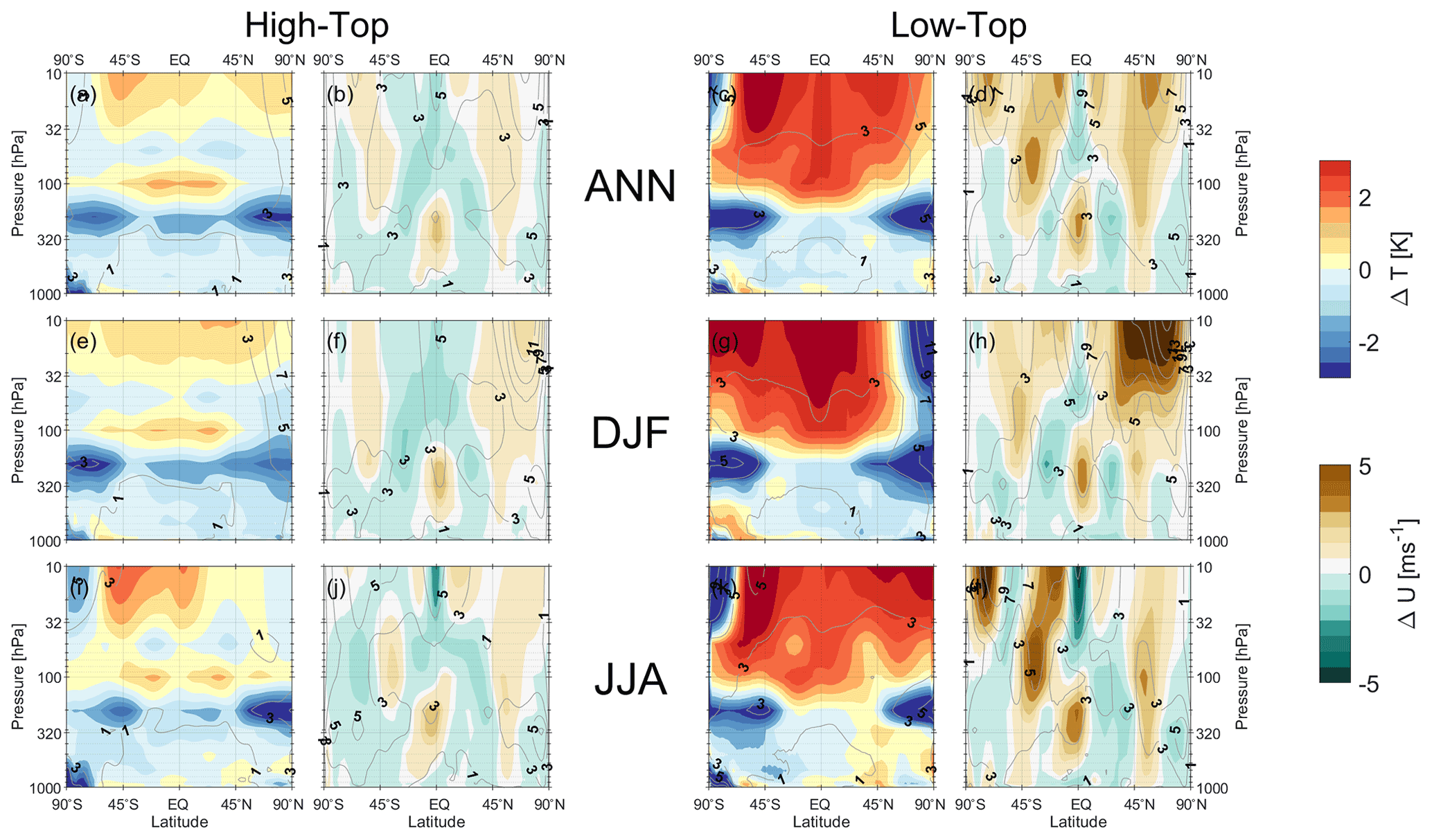
Figure 2 Zonal-mean (a, c, e, g, i, k) temperature and (b, d, f, h, j, l) zonal-wind biases as a function of pressure and latitude at a lead time of 4 weeks. Data are averaged over (a–d) the full annual cycle (ANN), (e–h) boreal winter (DJF), and (f–l) austral winter (JJA) and are shown separately for (a, b, e, f, i, j) high-top and (c, d, g, h, k, l) low-top models. The grey-line contours show the composites of mean absolute errors from each system.

The zonal-mean biases across the models are broadly consistent with the annual global-mean temperature biases shown above but reveal further important details about their vertical and meridional structures. Figure 2 shows the zonal-mean biases and mean absolute errors (MAEs) in temperatures and winds as a function of latitude and height for different seasons, composited for high- and low-top models at a lead time of 4 weeks. These biases and errors are shown for individual systems in the figures in the Supplement. We note that the interpretation of vertical variations in Fig. 2 and the supplemental figures requires some caution since the data from the S2S database are only provided on roughly three levels in the stratosphere (100, 50, and 10 hPa). Furthermore, since the UKMO and KMA systems both make use of the GloSea-5 model with the same atmospheric configurations, KMA has been left out of the high-top composite in Fig. 2 so as not to unfairly weight the high-top composite; as Figs. S12 and S14 in the Supplement show, these systems have nearly identical biases. The patterns of biases in temperatures and zonal winds are generally consistent across the high- and low-top composites with signatures of (1) global-mean warm biases in the stratosphere (consistent with Fig. 1), (2) cold extratropical upper-troposphere–lower-stratosphere (UTLS) biases in both hemispheres, (3) easterly wind biases in the tropical stratosphere, and (4) too strong/cold stratospheric polar vortices in the winter hemispheres. It is clear, however, that the biases and MAE in the low-top systems are generally much larger in magnitude despite the similarities in spatial patterns.

The cold extratropical UTLS and cold winter pole/strong polar vortex biases are recognized as long-standing issues in forecast and climate models. The former issue is generally thought to be related to excessive longwave cooling from a moist bias that is present in initial conditions, and/or it develops over time due to an inability to properly maintain the distribution of water vapor in the region of the tropopause (see, e.g., Bland et al., 2021, and references therein). Figure 2 and the supplemental figures show that these cold biases are still apparent in high-top models but are generally smaller in magnitude. For the Southern Hemisphere (SH) summer, the difference in the cold UTLS temperature bias between the high- and low-top systems is significant at 200 hPa (Fig. S15c in the Supplement). These differences may be related to the fact that the systems with high-top models generally have more model levels/higher vertical resolution, making them better able to represent processes in the tropopause region. The too strong/cold winter stratospheric polar vortex biases, particularly in the NH, reflect a lack of dynamical variability. Figure 2 shows that the low-top systems have higher MAE, more pronounced cold winter poles, and stronger polar vortex winds in both hemispheres; for the NH winter, the differences between the high- and low-top systems are significant at 10 hPa (Fig. S15c and d). These results are consistent with prior studies that find models with tops below the stratopause generally fail to realistically simulate stratospheric variability (e.g., Charlton-Perez et al., 2013; Shaw et al., 2014; Rao and Garfinkel, 2021a). There are multiple reasons why these biases are generally worse in low-top models, usually related to an underestimation of resolved/parameterized gravity wave drag (see, e.g., Sect. 3.3), as well as possible unphysical effects of the model lid (e.g., Shaw and Perlwitz, 2010; Richter et al., 2014).

The apparent easterly bias in the tropical stratospheric zonal winds across the high- and low-top systems represents a general bias among the models in representing the QBO. We examine these biases in the next section in more detail.

3.2 Biases related to the tropical stratosphere and QBO

The circulation of the tropical stratosphere is dominated by the QBO, and hence the zonal-mean biases in the tropics shown above must be partially related to each forecast system's ability to maintain the QBO from initial conditions. To the extent that S2S models can represent the QBO and its teleconnections accurately, the QBO could lead to more reliable predictions on subseasonal and seasonal timescales in the troposphere (Garfinkel et al., 2018; Merryfield et al., 2020). Therefore, we now consider whether this potential is realized by the S2S forecast systems. Unlike elsewhere in the paper, here our QBO analyses make use of the full hindcast periods available to each model to maximize the number of QBO cycles available when determining biases (see Table 1).

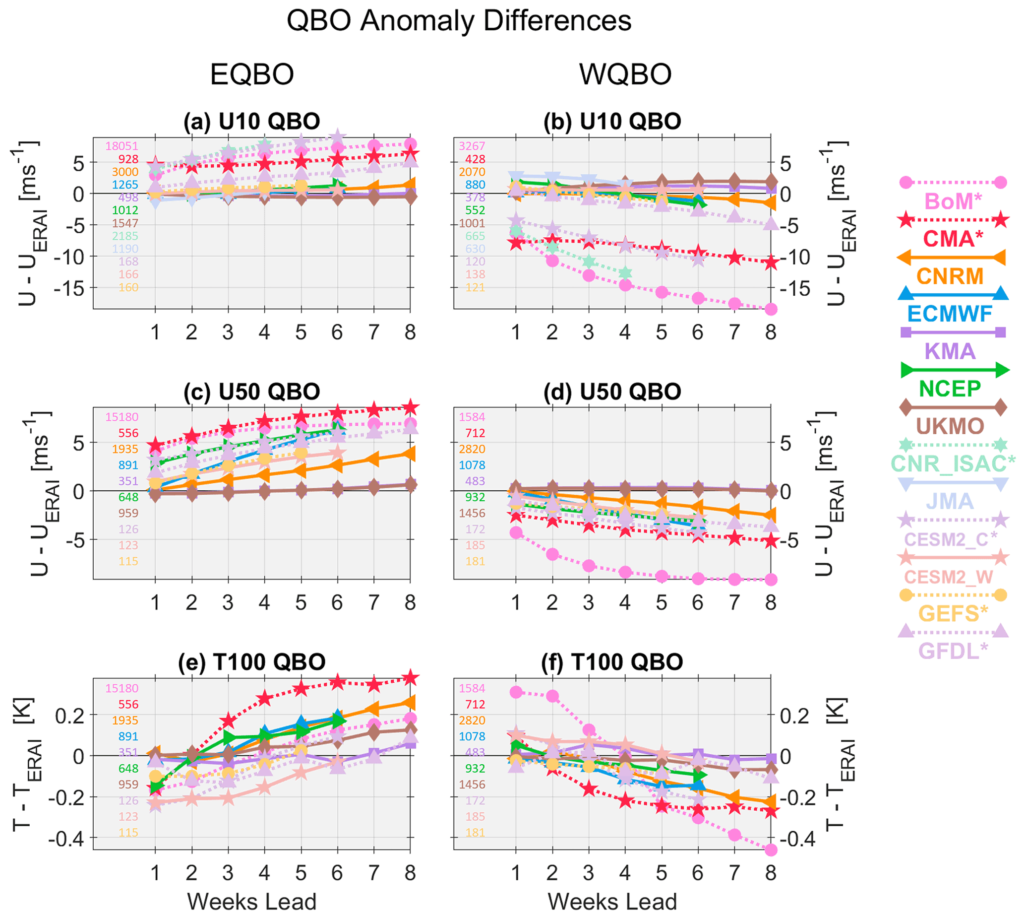
Figure 3 Time series of tropical stratospheric anomaly differences (from reanalysis) composited for easterly and westerly phases of the QBO in the subseasonal hindcasts. (a, b) QBO defined using 10 hPa, 5^∘ S–5^∘ N zonal wind; (c, d) QBO defined using 50 hPa, 5^∘ S–5^∘ N zonal wind; and (e, f) 100 hPa, 5^∘ S–5^∘ N temperature in the QBO phases defined using 50 hPa winds. All composites are based on November–February initializations only, with the number of initializations in each composite shown in each panel.

Figure 3 considers whether these models are capable of maintaining the anomalous QBO winds present in initializations from November through February (NDJF). In the top row, we composite hindcasts in which the zonal-wind anomalies (computed with respect to each model's climatology) at 10 hPa and 5^∘ S–5^∘ N averaged over the first 3 d of the hindcast exceed 3 m s⁻¹ are westerly QBO (WQBO) and those less than −3 m s⁻¹ are easterly QBO (EQBO); we subsample the ERA-I reanalysis anomalies to match the dates included in each model's composite before calculating differences. The middle row shows similar quantities but with the QBO-phase composites determined using the zonal-wind anomalies at 50 hPa instead. On subseasonal timescales out to 8 weeks, the reanalysis quantities for the QBO remain virtually constant (see Fig. S16 in the Supplement). At 10 hPa (Fig. 3, top row), systems with low-top models (dashed lines) clearly struggle to maintain the amplitude of both EQBO- and WQBO-initialized anomalies, which start out biased in week 1 by roughly 5 m s⁻¹ and decay with lead time compared to reanalysis by an additional 5 m s⁻¹ for EQBO and more for WQBO. The net effect is that the QBO signal (±10–20 m s⁻¹; Fig. S16a and b) is almost entirely lost for some of the low-top systems. The systems with high-top models generally show much slower and slighter decay, with relatively small anomaly differences from reanalysis close to 0 m s⁻¹ across lead times. At 50 hPa the reanalysis winds generally range from ±10–15 m s⁻¹ (Fig. S16c and d); in the forecasts (Fig. 3, middle row), even the high-top systems show an apparent decay of anomalies with lead time. The differences from reanalysis are slightly more apparent in the 50 hPa EQBO composite, for which a larger fraction of the model wind anomalies differ from reanalysis by 5 m s⁻¹ or more at the end of the forecasts compared to WQBO. The main exceptions are the UKMO and KMA systems, which share the same atmospheric models and perform well relative to the other systems as demonstrated by their reanalysis differences staying close to 0 m s⁻¹. Overall, the fact that the subseasonal forecast systems are generally better able to simulate and maintain the QBO in the middle stratosphere versus the lower stratosphere is similar to what has been found in climate models, seasonal forecast systems, and models participating in the “QBO initiative” (QBOi; Richter et al., 2020; Rao et al., 2020a; Bushell et al., 2022; Stockdale et al., 2022). This difference in success between the middle and lower stratospheric QBO could be related to several factors, including gravity wave parameterizations, the need for high vertical resolution in the lower stratosphere to realistically capture upward wave flux and subsequent downward QBO propagation, and possible influences from model vertical diffusion in the lower stratosphere (Geller et al., 2016; Garfinkel et al., 2022; Polichtchouk et al., 2021).

The QBO has been shown to influence tropical convection on subseasonal timescales, and one of the leading mechanisms for this effect is related to the QBO's mean meridional circulation, which leads to temperature (and buoyancy frequency) anomalies in the tropical tropopause layer that subsequently affect high clouds and convection (Gray et al., 2018). These relationships also underpin the QBO's observed relationship with the Madden–Julian Oscillation (MJO; Yoo and Son, 2016; Son et al., 2017; Lee and Klingaman, 2018; Martin et al., 2021a), which can modulate MJO forecast skill (Kim et al., 2019; Lim et al., 2019). To this end, we examine the associated temperature anomalies in the lowermost tropical stratosphere at 100 hPa (T100; bottom row of Fig. 3). These biases are composited based on the initial QBO wind anomalies at 50 hPa (consistent with the middle row). The temperature anomalies are proportional to the QBO-related shear in the lower stratosphere with typical EQBO/WQBO wind anomalies corresponding to cold/warm anomalies of ±0.5 K, as determined from reanalysis (Fig. S16e and f). These temperature anomalies are present in the initialized states of the models, with some systems overestimating the magnitude of the anomalies in week 1. However, in most of the systems, these T100 anomalies decay with lead time and eventually switch sign such that the models become warmer relative to reanalysis in EQBO and colder in WQBO. The rate of weakening differs among the models, with the low-top systems generally showing much more rapid decay of anomalies. There appears to be little difference between the EQBO and WQBO composites in the ability of models to maintain the tropical lower-stratosphere temperature anomalies. Underestimating the amplitude of the QBO in the lower stratosphere (in both winds and temperatures) down to the tropopause is an issue similar to that present in CMIP6 and QBOi models (Bushell et al., 2022; Richter et al., 2020), and may be a factor contributing to why many subseasonal forecast systems show insignificant relationships between the QBO and MJO (e.g., Kim et al., 2019).

Figure 4 As in Fig. 3 but for polar stratospheric quantities in QBO composites based on the initial 50 hPa winds from November and December initializations, including (a, b) zonal-mean zonal wind at 10 hPa, 60^∘ N, and (c, d) 100 hPa, 70–90^∘ N polar cap geopotential heights (Z100). The numbers of initializations in the composites are shown in each panel.

The QBO is known to have an important teleconnection to the boreal winter polar vortex known as the Holton–Tan effect (e.g., Holton and Tan, 1980; Baldwin et al., 2001; Calvo et al., 2007; Garfinkel et al., 2012; Anstey and Shepherd, 2014), in which weaker or stronger polar vortex winds preferentially occur with EQBO or WQBO winds in the lower stratosphere, respectively. Figure 4 shows the composite anomalies in 10 hPa polar vortex winds and 100 hPa polar cap geopotential heights (Z100) composited based on the 50 hPa QBO phase at initialization. Since the Holton–Tan effect develops in early winter and is most pronounced in midwinter, Fig. 4 is limited to forecast initializations within November and December, before the effect is strongly embedded in initial conditions. In the reanalysis EQBO composites, the weak vortex signal becomes apparent beyond roughly 3 weeks, with easterly wind anomalies on the order of 5–10 m s⁻¹ that are maintained at longer lead times (Fig. S17a in the Supplement). While most of the subseasonal forecast systems track reanalysis closely out to 3–4 weeks, it is clear that they underestimate the magnitude of polar vortex weakening (Fig. 4a), with winds that are too westerly at longer leads. The results for WQBO (Figs. 4b and S17b) are largely similar, with the subseasonal forecasts having an easterly wind bias at longer leads. The bottom row of Fig. 4 shows the anomalies in polar cap geopotential heights at 100 hPa, where persistent anomalies in the strength of the lower stratospheric vortex are more closely tied to surface-related impacts. Here the results are similar to the 10 hPa polar vortex winds, with most systems failing to match the change in amplitude of the anomalies with lead time, which can exceed ±40–60 m in reanalysis (Fig. S17c and d).

3.3 Northern Hemisphere polar vortex variability

Variability in the NH polar winter stratosphere primarily arises from extreme dynamical polar vortex events, including midwinter SSWs and strong vortex events. The occurrence of these events is generally associated with extremes in the upward wave fluxes that disturb the polar vortex, with SSWs and strong vortex events being preceded by extended periods of above- and below-normal wave driving, respectively (e.g., Polvani and Waugh, 2004). A typical metric for upward planetary wave flux is the meridional eddy heat flux, $v^{\prime }{T}^{\prime }$ (with v being the meridional wind, T the temperature, and the primes denoting deviations from the zonal mean). In models, such wave driving should be well represented, dependent upon the tropospheric variability and proper simulation of vertical wave propagation. There can also be significant variability among polar vortex events in terms of different characteristics, such as their timing, magnitude, persistence, and even polar vortex geometry (e.g., Karpechko et al., 2017). Importantly, the occurrence of such polar vortex events can lead to coupling with the troposphere that lasts for weeks to months; in forecast models, the occurrence of these events can improve tropospheric predictability by providing “forecast windows of opportunity” (e.g., Butler et al., 2019a, and references therein).

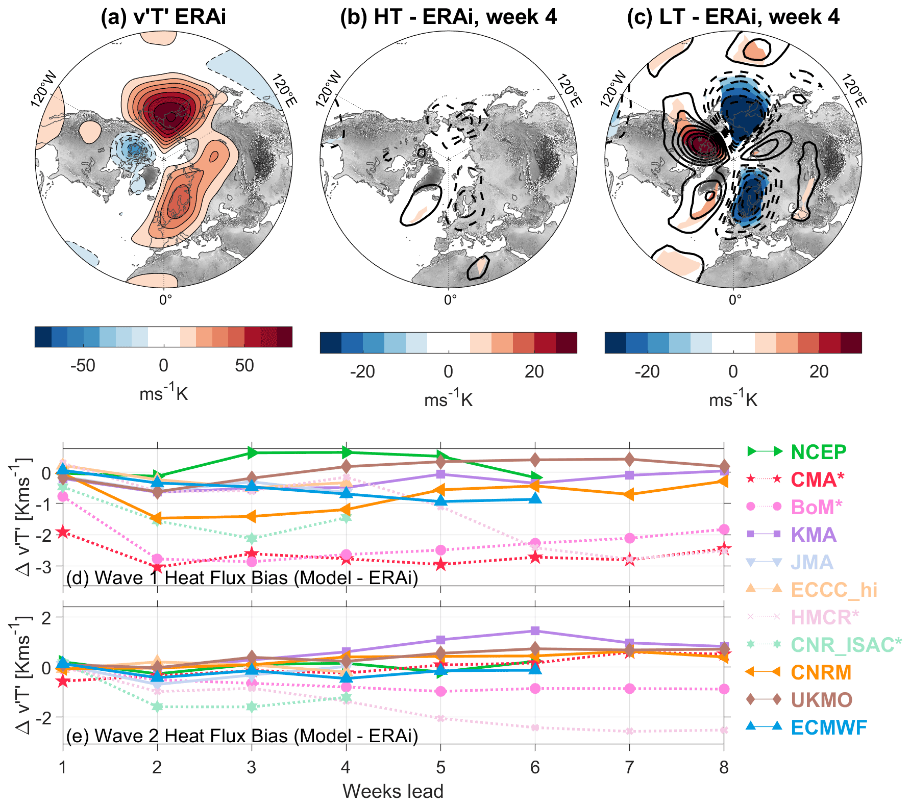
Figure 5 (a) The December–February climatology of ERA-I (“ERAi” in the figure) eddy heat fluxes, $v^{\prime }{T}^{\prime }$, at 100 hPa. (b) The high-top composite of week-4 eddy heat flux biases with respect to ERA-I from November–January initializations. Panel (c) is as in (b) but composited for the low-top models. In panel (a), the line and color-filled contours match the color-bar spacing of 10 K m s⁻¹; in panels (b) and (c), the line contours match the color-bar contour intervals of 5 K m s⁻¹, but colors are only shown where the biases are statistically significant at the 95 % level from a two-tailed Student's t test. (d) Time series of the difference between the S2S hindcasts and ERA-I for the wave-1 eddy heat flux averaged over 45–75^∘ N for lead times from 1 to 8 weeks. Panel (e) is as in (d) but for wave 2.

We first examine and compare biases in the NH eddy heat fluxes among the subseasonal forecast systems. Figure 5 shows the December–February eddy heat flux biases with respect to ERA-I at a lead time of 4 weeks. The climatological DJF 100 hPa heat flux from ERA-I is shown in Fig. 5a, while the high- and low-top composite biases are shown in panels b and c. The observed climatological heat fluxes show two centers of action, with one over the North Pacific and another over Scandinavia–Siberia. This pattern largely represents the influence of planetary-scale zonal waves 1 and 2, which generally have the most impact on the stratosphere. The mean biases in the subseasonal forecast systems strongly differ between the high- and low-top composites. The high-top systems underestimate heat fluxes in the Pacific region more than over Scandinavia–Siberia, which manifests as a slight negative bias in wave-1 heat fluxes (Fig. 5d), but none of the biases are statistically significant. In contrast, the low-top systems significantly underestimate heat fluxes in both regions while also overestimating heat fluxes over Canada and Greenland; the latter likely indicates that the low-top systems do not capture the region of negative heat fluxes seen in the ERA-I climatology, a region commonly influenced by downward wave reflection (Matthias and Kretschmer, 2020; Cohen et al., 2021; Messori et al., 2022).

These biases in regional heat fluxes are indicative of biases in the heat flux contributions from zonal waves 1 and 2, and thus we show the time evolution of these in Fig. 5d and e. In most of the models, the week-1 wave-1 heat flux biases are small in magnitude, except for low-top systems such as CMA and BoM. As mentioned above, the greater underestimation of heat fluxes over the Pacific in the high-top models is indicative of a slight negative wave-1 bias, which is most apparent in the CNRM and ECMWF systems. However, the low-top systems show negative biases that are much larger in magnitude from week 3 and beyond, especially in the BoM and CMA systems. Here the NCEP system stands out since it actually overestimates the wave-1 heat flux for weeks 3–5. The results are similar for the wave-2 heat flux biases in Fig. 5e, which shows the low-top systems more strongly underestimate the heat fluxes across lead times compared to the high-top systems. The high-top systems all show very small wave-2 heat flux biases out to about week 6, after which the CNRM, KMA, and UKMO systems have a slight positive bias. Overall these results reveal that the low-top systems consistently underestimate the contributions of planetary-scale waves to eddy heat fluxes in the lower stratosphere, which is consistent with the strong vortex/cold pole bias shown in the low-top zonal-mean composite from Fig. 2.

Figure 6 Probability of boreal (a, c, e, g, i) sudden stratospheric warmings and (b, d, f, h, j) strong vortex events, shown individually for composites of initializations within each month (rows) and weekly lead time (horizontal axis, alternating grey–white background shading within panels). For each model, the solid bars show the raw estimates, while the bold horizontal black lines indicate the probability determined after bias correction. The colored circles indicate the probabilities computed using ERA-I and subsampled to match the same dates from each individual set of model hindcasts.

The biases in the stratospheric background circulation (Sect. 3.1) and heat fluxes described above can affect the occurrence and timing of threshold events such as SSWs and strong vortex events. Figure 6 shows the probability of occurrence of 10 hPa 60^∘ N winds less than 0 m s⁻¹ (corresponding to SSWs) or greater than 41.2 m s⁻¹ (corresponding to strong vortex events) for different weekly lead times. These probabilities are composited based on initialization, so for instance, the week-4 values of the January initializations (Fig. 6e and f) include verification times from the month of February. The seasonal distributions from reanalysis (colored circles) indicate low probabilities of SSW events in early winter (November and December), with the highest occurrence of events being in late winter (January–March). Note that since the figure is composited based on initializations, the probabilities for March include verification times in April, and so the corresponding probabilities for easterly winds are likely influenced by final warmings. Regardless, this seasonal cycle is only partially reproduced in the subseasonal models, which particularly underestimate the probability of events for December and January initializations in weeks 3 and 4 and overestimate the probability for March initializations in weeks 3 and 4. This bias is in agreement with results from climate models (Ayarzagüena et al., 2020; Tyrrell et al., 2021), which tend to exhibit a peak in SSW occurrence in late winter instead of in January, and seasonal prediction models, which also fail to reproduce the SSW peak in January (Portal et al., 2022) despite the seasonal average of SSWs often being well reproduced (Domeisen et al., 2015). Interestingly, the NCEP system consistently predicts a higher occurrence of easterly winds than other systems. This means the NCEP system is more accurate for week-4 SSW risk forecasts initialized in December and January but then overestimates SSW probabilities in February and March. The NCEP system's higher prediction of easterly winds is possibly related to its significant weak vortex bias (see Fig. S13 in the Supplement), which may be linked to its overestimation of heat fluxes (Fig. 5d).

Strong vortex events (right column of Fig. 6) exhibit an entirely different seasonal cycle, with most events occurring between December and January (primarily due to the threshold-based definition and the climatological maximum strength of the vortex occurring in these months). Most models tend to underestimate the frequency of strong polar vortex winds for November and December initializations, particularly at weeks 3 and 4. There are some notable exceptions, including the CNR-ISAC, CNRM, GEFSv12, and CESM2-CAM systems, which all have substantial strong polar vortex biases in their wintertime zonal winds (Figs. S2, S5, S6, and S9 in the Supplement). For January initializations, most models instead overestimate the frequency of strong vortex winds beyond week 1 (Fig. 6f), which is also consistent with the general strong vortex biases evident in the model composites of Fig. 2.

In addition to the probability of the events from raw forecasts, the horizontal black lines in Fig. 6 indicate the probabilities estimated from bias-corrected forecasts (see Sect. 2.2 for details of the mean bias-correction process). The probability of both SSWs and strong vortex events in the bias-corrected hindcasts initialized in November, December, and January is generally either close to or smaller than the observed probabilities from ERA-I across all forecast systems. In most cases, this corresponds to an improvement over the raw forecasts. Especially for the prediction of SSWs for forecasts initialized in January (Fig. 6e), the mean bias correction clearly improves the estimates over those from the raw data, particularly for lead times of 3–4 weeks. However, the bias correction for late-winter/early-spring predictions (initializations in February and March, weeks 3 and 4) does not necessarily bring the easterly wind probabilities closer to observations. In some cases the bias correction increases the probability of events, even for systems whose un-corrected probabilities already closely match reanalysis. This may mean that model zonal-mean zonal-wind biases in late winter and early spring tend to not dynamically alter the probability of zonal-wind reversals at times when final warmings may be expected to occur. The exceptions here are the systems with the most severe biases, such as BoM and CNR-ISAC. Nevertheless and especially for early winter, the magnitude of zonal-wind biases clearly changes the probability of fixed-threshold events in most of the S2S systems. This supports the utility of bias correction for stratospheric S2S forecasts, albeit with some limitations. Furthermore, such bias correction has to be applied and interpreted with care, since the non-linear dynamics in the models evolve according to their own potentially biased mean states, and therefore, little can be said about potential tropospheric responses to such bias-corrected stratospheric forecasts.

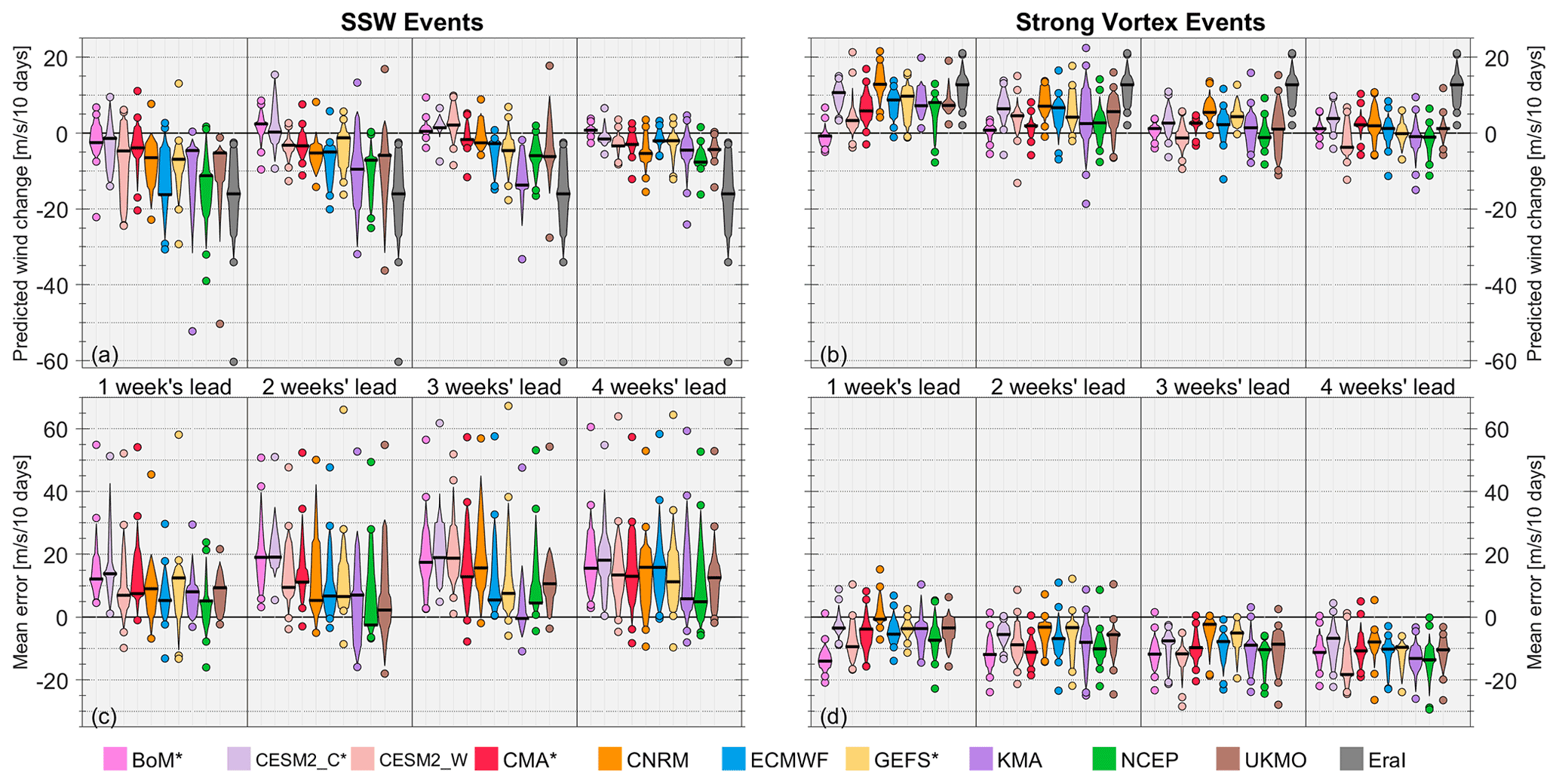
Figure 7 Distributions of the composited wind changes forecasted by each ensemble for forecast verification times surrounding (a, c) boreal sudden stratospheric warmings and (b, d) strong vortex events, composited over all such events in the 1999–2010 hindcast records. This corresponds to 11 SSW events and 13 strong vortex events across the boreal winters from 1999/2000 to 2009/10. Units are m s⁻¹ over the 10 d period centered on the observed event central dates within the forecasts or reanalysis. Within each section of each panel, data are shown as violin plots covering the 15 %–85 % range of wind changes or mean errors, with outliers outside this range indicated with individual colored circles and horizontal black lines indicating the median value. In panels (a) and (b) the quantities shown are raw values, while those in panels (c) and (d) are shown as deviations from ERA-I (EraI in the figure). Note that individual models may contain a slightly different number of samples, especially for longer lead times, due to the different hindcast lengths available for each system (see Table 1); in other words, some hindcasts do not fully cover the 10 d periods surrounding the observed SSWs and strong vortex events and are excluded.

There also exist biases in the magnitude of predicted events, even at relatively short lead times. In Fig. 6 we identified the probability of polar vortex events occurring in the subseasonal forecasts at different lead times; in Fig. 7 we instead focus on observed polar vortex events in the ERA-I record and assess the forecasted wind changes at verification times surrounding the observed events. Figure 7 shows the distributions of simulated wind changes associated with SSWs and strong vortex events (defined as in Sect. 2.2) in the 1999–2010 reanalysis record. The deceleration or acceleration associated with these events is measured by computing the change in the hindcast/reanalysis zonal-mean zonal wind at 10 hPa and 60^∘ N, at ±5 d around the ERA-I event onset dates; for the hindcasts, these are first computed individually for each ensemble member before being composited. Almost all systems underestimate the wind changes for both SSW and strong vortex events at all lead times, yielding dominantly positive and negative mean errors for SSWs and strong vortex events, respectively. However, the prediction of the observed magnitude of events clearly improves with decreasing lead time, as expected. At week-3 and week-4 lead times, the predicted wind change distributions among the systems are generally close to zero and exhibit small spread. This indicates that these models predict climatological zonal-mean zonal-wind values or only weak wind tendencies of the same sign as the events. This is not a shortcoming of the prediction systems but rather to be expected given that the typical predictability limit for these vortex events is about 2 weeks. Even within a lead time of 2 weeks, some systems still underestimate the magnitude and spread of the observed wind changes; many of these are the low-top models such as BoM, CESM2-CAM, and CMA. For SSWs, the ECMWF and NCEP systems have the smallest errors of around 5 m s⁻¹; for strong vortex events, the CNRM, CESM2-CAM, and GEFSv12 systems consistently have the lowest mean errors within 10 m s⁻¹ from 1–3 weeks, but these systems also have substantial positive zonal-wind biases. Figure 7c and d also highlight the disparity in the magnitude of wind changes between SSWs and strong vortex events; median errors for SSWs are on the order of 15–20 m s⁻¹ with outliers up to 60 m s⁻¹, whereas the range is much smaller for strong vortex events. This reflects the large and sudden deceleration of winds that occur during SSWs that (in absolute terms) is much larger than the acceleration of winds for strong events.

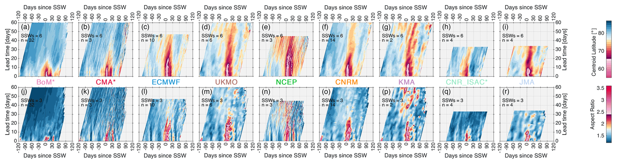
Figure 8 Predictions of the boreal stratospheric vortex (a–i) centroid latitude and (j–r) aspect ratio, computed at 10 hPa from hindcast geopotential height. Values shown are an average of all ensemble members over all (a–e, f–i) displacement and (j–n, o–r) split SSWs in the 1999–2020 record. Data are plotted against (horizontal axis) the SSW-relative day number and (vertical axis) model lead time. For each panel, the number of SSWs (“SSWs”) and number of ensemble members (“n”) are indicated at top left. The color-bar transitions to pink occur at thresholds of 66^∘ N for the centroid latitude and 2.4 for the aspect ratio.

Finally, we examine whether there are biases among the subseasonal models in forecasting the geometry of the polar vortex at times surrounding observed SSW events. The shape and location of the polar vortex are ultimately affected by the vertical wave activity that influences the occurrence and/or magnitude of SSWs. We examine vortex geometry using elliptical diagnostics, which provide quantities such as the vortex centroid latitude and aspect ratio (e.g., Waugh, 1997; Seviour et al., 2013) that can be used to quantify the displacement or stretch of the vortex during SSWs. We perform these calculations using the hindcast 10 hPa geopotential heights, assuming that the 30 km contour is representative of the vortex edge. Figure 8 shows the ensemble-mean predictions of the centroid latitude and aspect ratio diagnostics as a function of lead time and initialization with respect to composites of the central dates of displacement and split SSWs in 1999–2010. Note that the color bars of Fig. 8 transition to pink colors at 66^∘ N for the centroid latitude and at 2.4 for the aspect ratio, corresponding to the thresholds used in Seviour et al. (2013) to define displacement and split SSWs. For displacement events (Fig. 8a–i), most models capture a latitudinal deviation from the pole at long lead times of around a month, though with an underestimation of the magnitude of the displacement at lead times beyond 3 weeks. However, the BoM, CMA, and NCEP systems show signs of systematic biases in their predicted centroid latitudes. BoM and CMA (both low-top systems) show virtually no centroid latitude variability at longer lead times, with only the forecasts falling within about 2 weeks of the SSWs showing significant latitudinal displacements. On the other hand, NCEP appears to have a systematic bias toward a vortex that is too frequently displaced at longer lead times. While Fig. 8 is only focused on SSW events, the results for NCEP, BoM, and CMA are consistent with their climatological heat flux biases shown in Fig. 5; at longer leads, BoM and CMA consistently underestimate wave-1 heat fluxes, while NCEP consistently overestimates them.

In the case of vortex split SSWs (Fig. 8j–r), the high-top models perform much better relative to the low-top models, though still worse relative to displacement events. Vortex split events are known to be inherently less predictable than displacement events (e.g., Taguchi, 2018; Domeisen et al., 2020a), but the low-top models only show enhanced aspect ratios within a lead time of roughly 10 d. Of these, the BoM system shows large aspect ratios only in the initializations that are close to the onset dates. While the sample sizes here are quite small with only six displacement and three split events in the common time period under consideration, these results do show the signatures of the systematic biases among the modeling systems shown previously, particularly those for the wave-1 and wave-2 heat fluxes (Fig. 5).

3.4 Southern Hemisphere polar vortex variability

In the Southern Hemisphere (SH), stratospheric polar vortex variability is mainly associated with interannual variability in the timing of the springtime polar vortex breakdown (i.e., the final warming) sometime between November and January. Prior to the final warming, the SH polar vortex undergoes a downward shift in its location relative to its midwinter position (Mechoso et al., 1985). The downward shift of the polar vortex has been linked to a poleward shift of the SH eddy-driven jet in austral spring, while the timing of the polar vortex breakdown has been linked to the equatorward shift of the eddy-driven jet between November and January (Hio and Yoden, 2005; Byrne et al., 2017).

Given the above, the SH spring season can be regarded as a “window of opportunity” for more skillful tropospheric forecasts on S2S timescales provided that stratospheric variability is accurately represented. Indeed, previous studies have shown that the SH tropospheric variability during spring, prior to the polar vortex breakdown, can be predicted from stratospheric initial conditions in winter (Seviour et al., 2014; Lim et al., 2018; Byrne et al., 2019; Rao et al., 2020b; Oh et al., 2022). However, evaluations of individual seasonal prediction systems such as the ECMWF reveal unrealistic SH stratospheric variability and an inability to correctly represent stratosphere–troposphere coupling during austral spring, with likely impacts on the tropospheric mean state during that season (Polichtchouk et al., 2021).

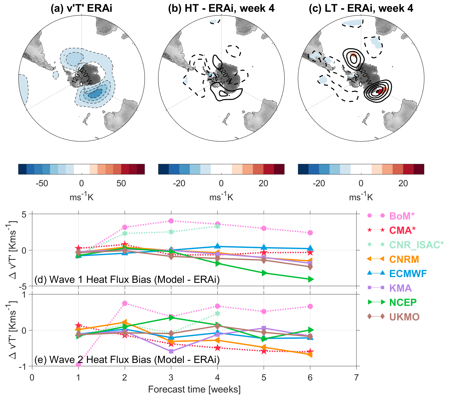
Figure 9 (a) The September–November climatology of ERA-I (ERAi in the figure) eddy heat fluxes, $v^{\prime }{T}^{\prime }$, at 100 hPa in the Southern Hemisphere. (b) The high-top composite of eddy heat flux model biases with respect to ERA-I from August–October initializations at a lead time of 4 weeks. Panel (c) is as in (b) but composited for the low-top models. In panel (a), the line and color-filled contours match the color-bar spacing of 10 K m s⁻¹; in panels (b) and (c), the line contours match the color-bar contour intervals of 5 K m s⁻¹, but colors are only shown where the biases are statistically significant at the 95 % level from a two-tailed Student's t test. (d) Time series of the difference between the S2S hindcasts and ERA-I for the combined wave-1 and wave-2 planetary wave heat flux over 45–75^∘ S, based on August–October initializations.

As with the NH, we first explore biases in the wave driving of the SH stratosphere, represented by the 100 hPa eddy heat flux, $v^{\prime }{T}^{\prime }$ (Fig. 9). In the SH, negative eddy heat fluxes are poleward and represent upward propagation of wave activity into the stratosphere. In ERA-I (Fig. 9a), the poleward eddy heat fluxes are largest over the Southern Ocean with local maxima south of Australia (150^∘ E) and downstream of the Antarctic Peninsula (30^∘ W). Eddy heat fluxes climatologically peak in amplitude in austral spring and are associated primarily with stationary waves of wavenumber 1 with a secondary role from transient waves (Randel, 1988). Similarly to the NH (Fig. 5), the spatial patterns of eddy heat flux biases strongly differ between the high- and low-top composites, particularly at longer lead times. In week 4 (Fig. 9c), the low-top composite shows positive biases over the two local maxima in the ERA-I climatology; these biases are primarily from the BoM and CNR-ISAC systems, which both have large positive biases over the region between Antarctica and Australia, projecting onto the wave-1 heat fluxes (see also Fig. 9d). In contrast, the pattern of biases in the high-top composite is much less coherent except for a relatively large region of negative biases between the southern tip of South America and the Antarctic Peninsula. The spatial patterns of SH heat flux biases shown for week 4 are largely consistent with those shown as a function of lead time (Fig. 9d and e). Among the low-top systems, BoM and CNR-ISAC show positive biases for both wave-1 and wave-2 heat fluxes beyond week 1 (indicating decreased poleward eddy heat flux); in contrast, the CMA system has relatively small wave-1 biases but too negative wave-2 heat fluxes beyond week 1 (indicating enhanced poleward eddy heat flux). Most of the high-top systems also have negative heat flux biases for both wavenumbers at longer leads, especially beyond week 4 for wave-1. Among these, NCEP shows the most negative biases for wave-1 heat fluxes, which nearly reach −5 K m s⁻¹ in week 6. The fact that the high-top systems seem to slightly overestimate SH upward wave fluxes could imply that these systems also have too high springtime variability in the SH stratosphere.

Figure 10 Interannual standard deviation of the Southern Hemisphere hindcast 50 hPa polar cap (60–90^∘ S) geopotential height for each model (colored lines) in comparison to ERA-I (black lines). The hindcasts closest to the first of each month are chosen for each model. The verification time range in each row spans a maximum of 8 weeks.

Following on from the SH eddy heat flux biases, Fig. 10 shows the interannual standard deviation of SH polar cap (60–90^∘ S) geopotential height at 50 hPa for each of the S2S systems based on initialization dates that are closest to 1 August, 1 September, 1 October, and 1 November. Here we consider the common hindcast period of 1999–2010 but exclude 2002, the year of the only major sudden stratospheric warming in the SH. In ERA-I, the observed interannual variability increases considerably from the beginning of October, peaking in mid-November and decaying thereafter. The hindcasts initialized in August and September present similar levels of variability to reanalysis up to early October; for initializations in early September, several models (CNRM, ECMWF, KMA, UKMO) even show an increase in variability at longer lead times. However, the difference between the models and observations increases for initializations in early October and November, with most models underestimating the observed variability beyond 4 weeks. For early-November initializations, most of the high-top models (with the exception of NCEP) underestimate the variability at shorter lead times from roughly week 2 onward. Clearly though, the low-top models show the most consistent underestimation across the different months and lead times; BoM and HMCR particularly show nearly flat variations, indicating that they do not simulate an appreciable seasonal cycle in variability. The overestimation of SH variability shown by NCEP from week 4 and beyond in October and November initializations is consistent with this system having the most negative heat flux biases in Fig. 9. Overall, because of the limited number of years in the comparison, most of these differences in variability with respect to reanalysis are not significant (not shown).

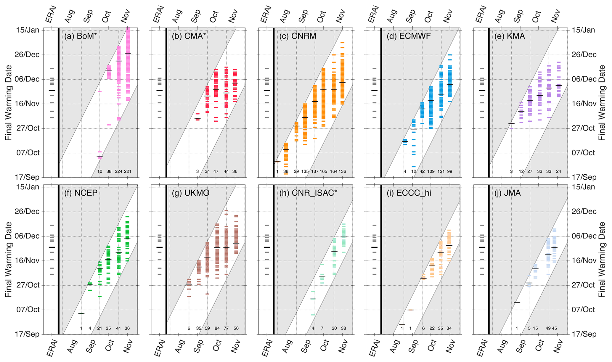
Figure 11 Plots showing the distribution of Southern Hemisphere final warming dates predicted by each S2S system. The reanalysis final warming dates from ERA-I (ERAi in the figure) are shown by the grey strips on the left side of each panel. The systems are composited based on initializations that fall closest to the beginning or middle of each month as specified on the x axis. The diagonal white region represents the approximate maximum forecast horizon for each system and initialization.

There are also biases in the timing of the seasonal breakdown of the SH polar vortex. Figure 11 shows histograms of the polar vortex breakdown dates across different initialization dates between August and November. Here we simply define the breakdown date as the first day of easterlies without subsequent return to westerlies at 10 hPa and 60^∘ S. For many of the models, forecasts initialized in early spring produce easterly winds toward the end of the forecast but at times that are much too early for the breakdown. This is a somewhat surprising result given that such early polar vortex wind reversals are rare in observations and expected to be rare in model simulations (e.g., Jucker et al., 2021). It is unclear, however, whether this behavior represents an early-breakdown bias among some of the forecast systems or whether these events represent SSWs for which the polar vortex would eventually recover if the forecasts continued in time. Regardless, these models produce early events that are generally not consistent with the observational record. Breakdown dates that fall within the ERA-I range are generally only produced for initializations on or after 1 October or once the end of the forecasts include the second half of December. An exception is the BoM model, which produces breakdown dates that consistently fall close to the end of its forecasts, resulting in a late-breakdown bias for initializations after October. Notably, free-running coupled climate models have a bias toward too late breakdowns of the SH polar vortex (Butchart et al., 2011; Rao and Garfinkel, 2021b); this suggests that information contained in the October initializations likely helps to constrain the S2S models and improve final warming estimates. Although stratospheric ozone is prescribed to climatological values in many S2S forecast systems, the strength of the initialized polar vortex winds in October likely contains information about relevant chemistry–climate feedbacks with stratospheric ozone that are well correlated to the timing of the breakdown date (Butler and Domeisen, 2021).

4 Discussion and conclusions

We have performed a comprehensive intercomparison of stratospheric biases in subseasonal forecast systems, with a core focus on systems that contribute to the S2S database (Vitart et al., 2017). Our results show the following:

• Forecast systems with low-top atmospheric models generally have the largest biases across the diagnostics examined for zonal-mean winds and temperatures, the QBO, meridional eddy heat fluxes, and the stratospheric polar vortices.

• Global- and annual-mean warm biases in the stratosphere tend to be most common across the different S2S forecast systems, though this can vary for different regions of the stratosphere in some cases (e.g., lower versus middle stratosphere).

• Too strong/cold wintertime polar vortices and too cold extratropical UTLS regions are common features across most of the systems in the zonal-mean temperature and zonal-wind biases.

• Tropical stratospheric anomalies associated with the QBO tend to decay with lead time to be too weak compared to reanalysis. For high-top systems, this issue is mostly only apparent in the lower stratosphere.

• Stratospheric polar vortex anomalies associated with different phases of the QBO (the Holton–Tan relationship) do develop in the forecast systems, but they are generally weaker than in reanalysis.

• In the NH, most S2S forecast systems do not capture the seasonal cycle of extreme-vortex-event probabilities; for example, the occurrence of SSWs and strong vortex events is underestimated and overestimated, respectively, for week-3–week-4 forecasts initialized in January. Similarly, the S2S systems generally underestimate the magnitude of wind changes associated with observed SSWs and strong vortex events, even at lead times within 2 weeks.

• In the SH, most systems generally underestimate the late-spring variability in the Antarctic polar vortex, particularly for initializations in October and November. However, many systems also simulate reversals in the 10 hPa 60^∘ S zonal-mean zonal winds for initializations in August and September, at times of the year when SH final warmings have not occurred in reanalysis.

These biases likely arise due to a combination of factors. While the physical processes that govern the evolution of the stratosphere are relatively well understood, they are generally not fully resolved within atmospheric models and are instead dependent upon model configurations (e.g., the height of model lids and vertical resolution) and simplified/parameterized processes (e.g., gravity wave drag and the representation of ozone). The resulting biases can affect both the mean state and the variability in the stratosphere and have potential consequences for subsequent coupling with the troposphere.

Several of the systems with the largest global- and annual-mean warm biases in the stratosphere are those in the NOAA family, including the high-top NCEP CFSv2 and the low-top GEFSv12 and GFDL-SPEAR; the others include the low-top BoM and CESM2-CAM. The only systems with global- and annual-mean cold biases are the ECMWF and CESM2-WACCM systems. It is unclear whether the warm biases in the NOAA systems are related to a common cause. While the GEFSv12 and NCEP CFSv2 models use similar physics packages, including ozone physics parameterizations and radiation packages, they do use different dynamical cores (Guan et al., 2022; Saha et al., 2006, 2014); similarly, GEFSv12 and the GFDL-SPEAR share the same FV3-based dynamical core, but SPEAR uses different physics packages and uses prescribed monthly ozone time series (Zhao et al., 2018; Delworth et al., 2020). The fact that the global- and annual-mean stratosphere should be in radiative equilibrium poses a strong constraint that biases are likely to be radiative in nature, but model dynamics related to horizontal and vertical resolution can also play a role, particularly at high resolutions (see, e.g., Polichtchouk et al., 2019). We note that the global-mean cold biases in the ECMWF system are likely dependent on the specific model cycles and that more recent versions likely have reduced cold biases following implementation of quintic vertical interpolation in the ECMWF model's semi-Lagrangian numerics (Polichtchouk et al., 2019).

The cold biases in wintertime polar cap temperatures (corresponding to stronger polar stratospheric winds) and cold biases in the extratropical upper troposphere–lower stratosphere are long-standing biases that are similar to what has been documented in other weather and climate models (Charlton-Perez et al., 2013; Bland et al., 2021). The stratospheric polar cap temperature biases generally point to dynamical influences related to planetary wave drag and parameterized gravity wave drag, since wave–mean flow interactions and the ensuing residual circulations are responsible for driving local zonal-mean temperatures away from radiative equilibrium. The cold extratropical UTLS biases, on the other hand, are likely to be radiatively driven, related to excessive leakage of water vapor into the lower stratosphere (e.g., Bland et al., 2021). Both of these issues are dependent upon vertical resolution, which likely explains why the biases in the low-top systems (which have fewer levels in the stratosphere and coarser resolution in the UTLS) are generally more severe than those in the high-top systems. Reducing such biases through model improvements is likely to have some impact on forecast skill in both the stratosphere and the troposphere since the latitudinal dependence of the temperature biases affect the distribution of winds (i.e., the tropospheric jets and stratospheric polar vortices). For instance, artificially bias correcting the extratropical UTLS humidity biases in the ECMWF forecast model was shown to remove the UTLS cold biases and moderately improve the skill of forecasts over Europe (Hogan et al., 2017).

The gradual decay of QBO anomalies with lead time toward each forecast system's own climatology is consistent with possible issues related to parameterized gravity wave drag. In models, the QBO has been shown to be most sensitive to parameterized non-orographic gravity wave drag (NOGWD) (e.g., Bushell et al., 2022), but other factors such as model vertical diffusion and resolution can also play a role in properly representing and maintaining the QBO, especially in the lower stratosphere (Garfinkel et al., 2022; Polichtchouk et al., 2021). However, documenting the specific model configurations and gravity wave parameterizations among the different forecast systems examined herein is beyond the scope of this study. Our results also showed that many of the S2S systems show a Holton–Tan response to the QBO wind phase in polar vortex winds and polar cap geopotential heights consistent with observations, but only for the first 2–4 weeks of the forecasts, after which the polar vortex anomalies decay.

To better understand the origin of stratospheric polar vortex biases, we examined the distribution and time evolution of NH lower stratospheric meridional eddy heat fluxes, which are a proxy for the vertical wave activity. These heat fluxes were generally more realistic in the high-top systems; the low-top systems showed considerable negative biases in heat fluxes in week 4 over the North Pacific and Scandinavia–Siberia. This suggests that, in combination with their limited representations of the stratosphere, these low-top systems have difficulties simulating realistic Rossby wave activity in the troposphere and/or their propagation and interaction with the mean flow (see, e.g., Schwartz et al., 2022). Thus, other biases documented for the low-top systems (such as those related to polar vortex winds and variability) are likely tied, to some extent, to these deficiencies. We documented similar behavior in the low-top composite of SH eddy heat fluxes, but the biases for the low-top systems were less robust and were particularly affected by the BoM system having large positive heat flux biases (indicating less upward wave driving in the SH).

Raw forecasts from the S2S systems do not accurately capture the seasonal cycle of boreal SSWs or strong vortex events. Removing the drift in the stratospheric zonal winds through simple bias correction does improve the probabilities for these events but primarily only for midwinter occurrences. While perfect prediction of such extreme polar vortex events is not feasible, ideally the statistics for their monthly occurrences derived from the hindcasts would more closely match those from reanalysis, especially at longer lead times and assuming similar levels of tropospheric “noise”. Furthermore, the underestimation of the magnitude of wind changes that occur surrounding extreme polar vortex events (even within 1–2 weeks of lead time) suggests that the S2S systems would likely have issues simulating downward coupling associated with such events. The persistence and magnitude of SSWs and strong vortex events are thought to comprise an important aspect that helps determine whether they lead to coupling with the troposphere (Maycock and Hitchcock, 2015; Karpechko et al., 2017; Charlton-Perez et al., 2018; Domeisen, 2019; White et al., 2019).

In the SH, a large fraction of the S2S systems seem to simulate early breakdowns of the SH polar vortex at 10 hPa, even for forecasts initialized in August and September. Because the forecasts are truncated in time, we cannot say whether these would be considered SSWs or final warmings, but nonetheless our results reveal that false-positive easterly wind events are relatively common in the S2S hindcasts. Such frequent and early reversals in the SH springtime stratospheric circulation are not a phenomenon seen in observations.

Our results show that many of the mean state biases become more sizable with increasing lead time (as expected), especially around weeks 3 to 4. Many of the S2S systems considered herein also make forecasts well beyond 4 weeks; on these extended timescales, such biases are likely to have more substantial impacts on stratosphere–troposphere coupling. While a fully unbiased model will not be possible to achieve, it is still desirable for models to (1) minimize mean state stratospheric biases so that the stratosphere represents a more accurate upper boundary condition for the troposphere and (2) have similar variability (in a statistical sense) to observations in the stratosphere so that ensemble spread properly accounts for potential outcomes. For example, forecasts from a model with a strong NH polar vortex bias could simply be post-processed with bias correction to improve the prediction for a SSW (Fig. 6); however, if the polar stratospheric winds stay westerly in the actual model simulation, then that would represent a different dynamical regime for stratosphere–troposphere coupling compared to the model actually simulating a transition to stratospheric easterlies (since easterly winds effectively shut off vertical propagation of Rossby waves).

This study primarily focuses on biases among S2S models within the stratosphere. We have shown that large biases are present throughout the stratosphere, linked to a range of stratospheric phenomena in the tropics and the extratropics of both hemispheres. To our knowledge, this is the first systematic assessment of such biases in the stratosphere and of processes affecting the stratosphere in a multi-model study of subseasonal-to-seasonal prediction systems. In a follow-up companion study as part of the same SNAP effort, we more closely examine how biases in the stratosphere, such as those identified herein, are linked to coupling with the troposphere and its predictability.