the Creative Commons Attribution 4.0 License.
the Creative Commons Attribution 4.0 License.
 | 02 Feb 2023
Vortex streets to the lee of Madeira in a kilometre-resolution regional climate model
Qinggang Gao
Christian Zeman
Jesus Vergara-Temprado
Daniela C. A. Lima
Peter Molnar
Christoph Schär
Atmospheric vortex streets are a widely studied dynamical effect of isolated mountainous islands. Observational evidence comes from case studies and satellite imagery, but the climatology and annual cycle of vortex shedding are often poorly understood. Using the non-hydrostatic limited-area COSMO model driven by the ERA-Interim reanalysis, we conducted a 10-year-long simulation over a mesoscale domain covering the Madeira and Canary archipelagos at high spatial (grid spacing of 1 km) and temporal resolutions. Basic properties of vortex streets were analysed and validated through a 6 d long case study in the lee of Madeira Island. The simulation compares well with satellite and aerial observations and with existing literature on idealised simulations. Our results show a strong dependency of vortex shedding on local and synoptic-flow conditions, which are to a large extent governed by the location, shape and strength of the Azores high. As part of the case study, we developed a vortex identification algorithm. The algorithm is based on a set of criteria and enabled us to develop a climatology of vortex shedding from Madeira Island for the 10-year simulation period. The analysis shows a pronounced annual cycle with an increasing vortex-shedding rate from April to August and a sudden decrease in September. This cycle is consistent with mesoscale wind conditions and local inversion height patterns.
- Article
(18142 KB) - Full-text XML
- BibTeX
- EndNote


Flow around isolated mountainous islands can lead to the formation of atmospheric vortex streets. Favourable conditions for the formation of vortex streets are quasi-steady upstream winds and a well-mixed planetary boundary layer capped by a thermal inversion below the island top (Etling, 1989).
Despite a striking similarity with the classic Kármán vortex street (Kármán, 2013), atmospheric vortex streets have different vorticity generation and decaying mechanisms. While Kármán vortex streets result from the instability of the wake behind cylinders in uniform laboratory flows, atmospheric vortex streets form in a stably stratified (a stratification below and above the inversion layer) turbulent flow passing asymmetric flat obstacles. The wake vorticity of Kármán vortex streets is generated by a viscous boundary layer, whereas vortex shedding can also be observed with free-slip boundary conditions in 3D numerical simulations. Atmospheric vortex shedding is speculated to be a result of potential-vorticity creation (Etling, 1989) and tilting of baroclinically generated horizontal vorticity under the deformation of isentropes that can be predicted by linear gravity wave theory (Smolarkiewicz and Rotunno, 1989). Wake patterns and vertical variations in Kármán vortex streets in unstratified fluids and a non-rotating reference frame depend solely on the Reynolds number Re. In contrast, atmospheric vortex streets are also characterised by the Froude number Fr, Rossby number Ro, and Strouhal number St (Horváth et al., 2020), whose definitions are given in Sect. 2.3.
Many studies focused on one or several specific aspects of vortex streets, which can be roughly divided into three categories: geometry, kinematics and dynamics.
Geometry describes the shape of individual vortices and vortex streets. The total length of vortex streets can reach 400 km or more (Etling, 1989), which indicates a lifetime of individual vortices of over 10 h considering a mean flow advection velocity of 10 m s−1. Based on satellite images from the Aqua and Terra Moderate Resolution Imaging Spectroradiometer (MODIS) satellites, Young and Zawislak (2006) investigated aspect ratios of vortex streets, i.e. the ratio of the distance between two vortex tracks to the distance between neighbouring like-rotating vortices. They reported higher ratios (0.36–0.47) compared to the value 0.28 derived by Kármán (2013) for Kármán vortex streets.
Kinematics of vortex streets include the shedding frequency and advection velocity of vortices. Using the Weather Research and Forecasting (WRF) model, Nunalee and Basu (2014) performed a detailed analysis of the Strouhal number. The Strouhal number represents a direct relation between vortex-shedding frequency, wind velocity and the crosswind island diameter at the inversion base. Tsuchiya (1969), using satellite images in the wake of Cheju Island, South Korea, reported that the advection velocity of vortices approximates 76 % of the undisturbed flow when the aspect ratio is 0.332.
Dynamics of vortex streets refer to vortex generation, shedding and decaying mechanisms. Heinze et al. (2012) employed an idealised large eddy simulation to study the azimuthally averaged structure of vortices. They found a warm core with convergence at the surface and divergence at the vortex top and suggested that a lower inversion at the vortex centre might explain cloud-free eyes in observations. From a mathematical perspective, the vertical vorticity can be derived from turbulent stresses and the tilting of horizontal vorticity (Epifanio, 2015; Rotunno et al., 1999). Schär and Smith (1993a) performed numerical simulations of a single layer of symmetric shallow-water flow past a circular mountain in a non-rotating environment with a frictionless surface. They proposed two mechanisms for the production of potential vorticity. First, internal dissipation, which is derived from a theory indicating that the steady-state Bernoulli function, is the stream function of the total vorticity flux. Second, flow separation leads to the joining of two flow streams with different values of the Bernoulli function. Subsequently, Schär and Smith (1993b) relaxed the symmetric flow conditions and analysed observed vortex streets with instability theory. With continuously stratified-flow models, Schär and Durran (1997) used the dimensionless mountain height to identify different flow conditions that are conducive for vortex shedding and gravity wave breaking, respectively. They suggested the generalised Bernoulli theorem (Schär, 1993) for the explanation of potential-vorticity generation. The dynamics of shedding in geophysical wakes are very similar to those of homogenous wakes, which have been well documented (Epifanio, 2015).
However, the study of vortex shedding in the lee of isolated islands is still limited by the availability of wind fields with high spatial and temporal resolutions. Satellite images of stratocumulus clouds, which are capped by an inversion base and can act as tracers of vortex streets, have been widely used for the study of vortex shedding (Young and Zawislak, 2006; Etling, 2019). They can provide information about geometric characteristics of vortex streets through daily snapshots in the case of polar-orbiting satellites such as MODIS Terra and Aqua, but they are restricted to cloudy conditions (Young and Zawislak, 2006). With cloud motion winds and ocean surface winds from the Advanced Scatterometer (ASCAT), Horváth et al. (2020) reported an asymmetric vortex decay with larger peak vorticity in cyclonic eddies than in anticyclonic eddies at Guadalupe Island. They argued that it is ascribed to Guadalupe's non-axisymmetric shape and Earth's rotation, where the latter factor is also supported by experiments of Ruppert-Felsot et al. (2005). Ito and Niino (2015) adopted a non-hydrostatic mesoscale model for numerical simulations of vortex streets in the lee of Cheju Island. They speculated that vortices are more likely generated through gravity wave breaking and the baroclinicity of flows over mountains than through viscous boundary layers. The importance of air–sea interactions on the wake patterns of Madeira Island was studied using the WRF numerical model by Caldeira and Tomé (2013). They proposed that the enhanced vertical mixing by increased sea surface temperature (SST) could lead to the erosion of the inversion base and a transition from vortex shedding to a long straight wake. Aerial observations were employed for the study of atmospheric wakes in the lee of Hawai'i (Smith and Grubišić, 1993) and Madeira Island (Grubišić et al., 2015). Grubišić et al. (2015) recommended potential vorticity, which can be generated by gravity wave breaking and is conserved in an adiabatic and inviscid flow, for the study of vorticity sources rather than the non-conserved vertical vorticity.
The impacts of vortex streets on the atmosphere and ocean have received relatively little attention. Using the Regional Ocean Modeling System ocean circulation model, Couvelard et al. (2012) investigated the influence of wakes induced by Madeira Island on the ocean-eddy generation with an eddy-tracking algorithm developed by Nencioli et al. (2010). They proposed that the island-induced wind wake contributes to oceanic surface kinetic energy and vorticity, as well as the generation and containment of ocean eddies. Nunalee et al. (2015) used a coupled mesoscale model and ray-tracing framework to explore kilometre-scale optical refractive perturbations caused by wake vortices of three islands. These perturbations are crucial for long-range optical communication systems that depend on precise laser guidance. Their study highlights the necessity of considering heterogeneous atmospheres (especially in the presence of vortex streets) for studies on optical wave propagation. With a focus on atmosphere–ocean interactions, Azevedo et al. (2020) studied the detailed responses of upper-oceanic profiles of temperature, salinity and turbulence to the Madeira warm wakes, which mainly result from intense solar radiation in cloud-free conditions.

Figure 1(a) The 12 km (CPS12) and 1.1 km (CRS1) COSMO model simulation domains and the location of the Madeira and Canary archipelagos. (b) Topography of the Madeira Archipelago with 30 m horizontal resolution from the European Environmental Agency under the GMES RDA (Global Monitoring for Environment and Security Reference Data Access) project. The grey shading shows the region with decadal model outputs in all 60 (61) vertical model layers (levels). The Funchal radiosonde data from IGRA 2 (Integrated Global Radiosonde Archive) were used to calculate the inversion height. A red ellipse e1 was fitted to the topography of Madeira using a Gaussian mixture model. The blue ellipse se was obtained by scaling e1 to of its area and then shifting along its minor axis for the length of its minor axis; se was employed to extract decadal 3D upstream conditions, which are only available within the grey-shaded area in (b). It is important to mention that these upstream conditions cannot be assumed to be undisturbed due to the proximity of se to the island. The altitude of two mountain peaks indicated by black triangles is used to compare with the inversion height. (c) The topography with a horizontal grid spacing of 1.1 km used in CRS1. The geographic map is from Natural Earth.
In this study, we focus on vortex streets in the lee of Madeira Island. It involves not only a case study as in most previous studies but also a climatology over 1 decade. The Madeira Archipelago is located near the northwestern African coast and forms part of Macaronesia. The weather and climate patterns in Macaronesia are mainly influenced by the subtropical semi-permanent Azores high-pressure system (Davis et al., 1997), prevailing northeasterly trade winds (Cropper and Hanna, 2014), local orographic characteristics (Carrillo et al., 2016), surrounding ocean currents and Sahara dust advection (Cropper, 2013). Madeira Island is the largest (740 km2) and highest (1862 m) island in this archipelago and the major source of atmospheric flow disturbances, while Porto Santo and Desertas play a minor role due to low altitudes. Madeira Island experiences less precipitation in summer than in winter. This can be mostly attributed to the more northern position of the Intertropical Convergence Zone (ITCZ) in summer and its associated dry region from the Hadley circulation. More precipitation is observed in the north or northeast windward regions than in the lee sides due to prevailing northeasterlies and orographic lifting (Cropper, 2013). The choice of Madeira Island for enhancing our understanding of land–atmospheric interactions is justified by its good isolation from continents, clear dynamical effects created by its topography and the vulnerability to extreme weather events induced by its geographical conditions (Ramos et al., 2018).
Plenty of theoretical studies have been devoted to the dynamics of vortex streets, and many observational studies concentrated on the geometry and kinematics. Nevertheless, they usually relied on limited case studies and idealised numerical simulations. This study contributes to this research field with realistic simulations of the real atmosphere and a vortex identification algorithm. This algorithm allowed us to investigate the climatology of vortex shedding to the lee of Madeira.
2.1 Model simulations

Figure 2(a) The grey shading shows the region used for subsequent analysis. The red ellipses e2 and e3 were obtained by shifting e1 as defined in Fig. 1b along its minor and major axes to extract upstream and undisturbed flow conditions, respectively. The dashed black and red polygons were used for vortex identification in Sect. 2.4. (b) An example of vortex streets to the lee of Madeira is visible through stratocumulus clouds using the data product MOD021KM from the MODIS Terra satellite (Savtchenko et al., 2004). Such pictures can be viewed directly on the website of NASA Worldview (https://worldview.earthdata.nasa.gov, last access: 30 January 2023). The geographic map is from Natural Earth.
We used the non-hydrostatic Consortium for Small-scale Modeling model in climate mode (COSMO-CLM Baldauf et al., 2011; Rockel et al., 2008). Specifically, we employed a refactored version of COSMO-CLM 5.09, which has been ported to run on hybrid GPU–CPU architectures in a joint effort between MeteoSwiss, the ETH-based Center for Climate Systems Modeling (C2SM) and the Swiss National Supercomputing Centre (CSCS) (Fuhrer et al., 2014, 2018). In COSMO, a third-order Runge–Kutta split-explicit scheme is used for integrating compressible Euler equations (Wicker and Skamarock, 2002). A fifth-order upwind scheme is used for horizontal advection, and an implicit Crank–Nicolson scheme is adopted for vertical advection. The model is equipped with a full set of parameterisation schemes (see Ban et al., 2014). We used a horizontal grid spacing of 1.1 km for a convection-allowing simulation (CRS1) over east Macaronesia (1100 km×1100 km) as shown in Fig. 1a. This simulation was run without employing the shallow- and deep-convection schemes. Lateral boundary conditions were provided by a convection-parameterising simulation with a horizontal grid spacing of 12 km (CPS12) driven by the ERA-Interim reanalysis with 6-hourly frequency (Dee et al., 2011).
The simulation domain was defined relative to a rotated north pole at 43∘ N and 170∘ W and contains 60 vertical layers up to 23.5 km altitude. The thickness of each layer widens from 20 m at the surface to around 1200 m near the model top. At the top of the model domain, we used implicit Rayleigh damping for the vertical velocity following Klemp et al. (2008) to prevent the reflection of upward-propagating gravity wave energy. CPS12 spanned from January 2000 to December 2015 including a spin-up period of 5 years, while CRS1 run from November 2005 to December 2015 and was initialised for 2 months before the analysis period to ensure a proper adjustment of the soil moisture (Ban et al., 2015). Both simulations provide hourly outputs on selected vertical levels over the entire respective simulation domains, and CRS1 also provides hourly data on all model levels over a smaller region indicated by grey shadings in Fig. 1b. While the wind data are available at altitudes of 10 and 100 m for the whole domain in CRS1, 100 m winds at 1.1 km horizontal grid spacing were used for our vortex-shedding analysis. For the case study in Sect. 3.2, we restarted the model simulation from 1 August 2010 at 00:00 UTC to generate 3D hourly data at a vertical interval of 100 m up to 5 km above the surface over the entire simulation domain of CRS1. Unless explicitly specified, the data used for analysis come from the original decadal CRS1.
Figure 1b shows the digital elevation model of the Madeira Archipelago with a horizontal resolution of around 30 m based on data from the European Environment Agency (https://sdi.eea.europa.eu, last access: 30 January 2023). We fit an ellipse centred at 32.74∘ N, 16.99∘ W with an area of about 800 km2 to Madeira Island using a Gaussian mixture model (Reynolds, 2015). The length of the major and minor axes of the ellipse are about 51 and 20 km, respectively. The minor axis is oriented at 79∘ and is approximately parallel to the prevailing trade winds. Figure 2a shows the model domain of CRS1 used for analysis, where we excluded 80 grid points at the lateral boundaries to eliminate any effect of the relaxation zone. In addition to the original ellipse e1 fitted to Madeira Island, we shifted it along its major and minor axes to extract upstream conditions at e2 centred at 33.01∘ N, 16.94∘ W and undisturbed flow conditions at e3 centred at 32.48∘ N, 15.66∘ W. An example of vortex streets in the leeward of Madeira Island is shown in Fig. 2b.
2.2 Observational data sources
In addition to model simulations, we explored multiple observational data sources for validation or comparison. The ERA-Interim reanalysis (Dee et al., 2011), with a horizontal grid spacing of about 79 km and a frequency of 6 h, was used to provide initial and boundary conditions for CPS12. For data analysis, we employed the ERA5 reanalysis (Hersbach et al., 2020), which is also produced by the European Centre for Medium-Range Weather Forecasts (ECMWF) and embodies hourly climate records at a higher horizontal grid spacing of around 31 km.
ASCAT is a C-band (5.255 GHz) fan-beam scatterometer system on polar-orbiting meteorological operational (Metop) platforms from the European Organisation for the Exploitation of Meteorological Satellites (EUMETSAT) (Figa-Saldaña et al., 2002). The primary mission of ASCAT is to provide 10 m global ocean wind vectors that are mainly used for assimilation in numerical weather prediction models. On ASCAT, six antennas cover two 550 km swaths with an interval of 360 km at a minimum orbit height of 822 km. A wind product, at a resolution of 25 km on a 12.5 km nodal grid, is generated from ASCAT Level 1b data using an empirical geophysical model function by the Ocean and Sea Ice Satellite Application Facility (OSI SAF). However, we used ASCAT Wind Data Processor (AWDP) software to derive wind data from measurements of ASCAT on board the Metop-A satellite at a higher resolution of around 17 km on a 6.25 km grid to provide more details about vortex streets (Vogelzang et al., 2017). When discussing vortex streets, we refer to modelled vortices by default; otherwise, we stress that the vortices are based on observations. Note that although the terms horizontal resolution and grid spacing are often used interchangeably (also in our study), they are different for ASCAT wind products and the products introduced below, as their values at each grid are derived by aggregating observations from surrounding grids.
For the comparison of vortex streets in simulations and the real atmosphere, we employed the high-rate SEVIRI (Spinning Enhanced Visible and InfraRed Imager) Level 1.5 image data of the geostationary satellite Meteosat-9 in the Meteosat Second Generation (MSG) from EUMETSAT (Schmetz et al., 2002). These data provide high-rate transmissions in 12 spectral channels covering 81∘ S–81∘ N, 79∘ W–79∘ E every 15 min. They have a sampling distance of 3 km and a horizontal grid spacing of 4.8 km at the sub-satellite point and a sampling distance of 4 to 5 km in our analysis region. An introduction to create and interpret standard RGB images from METEOSAT/SEVIRI can be found on the website of an international training project EUMeTrain founded by EUMETSAT (https://www.eumetrain.org, last access: 30 January 2023). We used the Natural Colour RGB for daytime (08:00–19:00 UTC) and the Night Microphysics RGB for nighttime.
Vertical temperature profiles from radiosonde observations at Funchal and Tenerife on a daily (normally at 12:00 UTC) and twice-daily (normally at 00:00 and 12:00 UTC) basis, respectively, from the Integrated Global Radiosonde Archive (IGRA) version 2 (Durre et al., 2006) were explored for a decadal climatology of inversion height. The location of Funchal radiosonde station is shown in Fig. 1b. As the geopotential height is often not available at reported pressure levels, it was computed using the hydrostatic relation (Durre and Yin, 2008). Although IGRA V2 provides the inversion height defined as the height of the warmest temperature in the sounding, we estimated it based on the definition from Kahl (1990), i.e. the lowest layer where temperature increases with height.
To validate simulated precipitation patterns, we used a dataset of conventional meteorological surface stations. The network contains 17 stations in the height range 25–1799 m. Most stations cover at least 5 years of the simulation period 2006–2015. The validation of precipitation against this dataset is conducted following the method described in Ban et al. (2020). That is, CPS12 model outputs are interpolated to station sites with nearest-neighbour interpolation, and for CRS1 the grid cell with the smallest altitudinal difference within a 4 km radius is selected for comparison.
2.3 Basic flow parameters
Following Snyder et al. (1985) and Heinze et al. (2012), the Froude number Fr was defined here as the ratio of inertial to buoyancy forces. In the case of a uniformly stratified airstream, it is given by , where N denotes the Brunt–Väisälä frequency, U is the upstream wind speed and hm is the mountain height. In some studies, the inverse of Fr was alternatively used and referred to as the dimensionless mountain height, i.e. .
The concept of the dividing streamline hds is commonly used in the analysis of flow past 3D topography. Here the height of this streamline hds is the upstream height that separates the streamlines passing over a 3D hill in a stably stratified flow from those passing around the hill. hds can be calculated based on Sheppard's energy theory (Sheppard, 1956): upstream air parcels at an altitude above hds would have sufficient kinetic energy to surmount the island, whereas below hds the flow is quasi horizontal around the island. Sheppard's energy theory assumes that all kinetic energy is converted to potential energy, and thus hds provides the lowest possible dividing streamline height. In the case of general upstream profiles U(z) and N(z), hds can be estimated from (Heinze et al., 2012)
where N(z) is the Brunt–Väisälä frequency defined as
Here g=9.81 m s−2 is the gravitational acceleration and θ(z) is the upstream potential temperature.
For upstream profiles of uniform N and U, hds can be obtained analytically as (Sheppard, 1956)
In atmospheric flows past 3D obstacles, vortex shedding occurs at Fr<0.4 (Etling, 1989), which appears to be roughly consistent with the laboratory experiments of Hunt and Snyder (1980). These results are also consistent with idealised numerical experiments using free-slip lower boundary conditions (Schär and Durran, 1997). For instance, Schär and Durran (1997) found vortex shedding for , while for there was nonlinear flow over the topography with gravity wave breaking and no vortex shedding.
However, the validity of Sheppard's energy theory was questioned by Smith and Gronas (1993) from a theoretical perspective. They argued that the deceleration of air parcels approaching the mountain is due to the pressure gradient associated with a hydrostatic gravity wave aloft, rather than due to vertical displacements of air parcels. Therefore, relationships between the dividing streamline height and vortex shedding should be investigated and interpreted with caution.
In our realistic simulation, N and U vary vertically, so we approximated Eq. (2) as
for the estimation of hdim, where hsurf denotes the surface height. Likewise, U and θ are expressed as the vertical average of wind velocity and potential temperature below hm, respectively.
The Rossby number is a dimensionless parameter for rotating reference frames. It is defined by the ratio between inertial force and Coriolis force as
where L is the relevant spatial scale and f=2Ωsin ϕ is the Coriolis parameter with s−1 being the rate of Earth's rotation and ϕ being the latitude.
Another important parameter, defining the dimensionless shedding frequency of vortices, is the Strouhal number, defined as
where D is the width of the island perpendicular to the wind direction at the inversion base and T is the shedding period between two successive vortices on the same side of obstacles.
2.4 Rule-based vortex identification
In this section, we introduced a rule-based vortex identification algorithm consisting of wavelet analysis and a series of criteria. The central idea of our algorithm is inherited from McWilliams (1990). He suggested judging the reliability of an algorithm in terms of both the prior plausibility of criteria and the posterior performance.
Several concerns in designing criteria are illustrated below. To extract individual vortices, we firstly denoised the spatial field of relative vorticity using wavelet analysis (Doglioli et al., 2007), of which theoretical and technical aspects are presented in Appendix A. Although in the case of ocean eddies, it is more objective to determine vortex boundaries based on closed streamlines (Nencioli et al., 2010), this method does not apply to atmospheric vortices due to strong background winds. As older shed vortices have a smaller area with relative vorticity above a given threshold, the main challenge is to separate small vortices from noise. Accordingly, we intentionally put stricter constraints on smaller vortices. The selected criteria are presented and explained below, and the order is designed to maximise computational efficiency.
-
Minimum magnitude of absolute values of relative vorticity for a vortex at a height of 100 m: s−1.
This step identifies grid cells that could belong to a vortex and clusters adjacent grid points above a threshold. The cell identification is based on a cloud identification algorithm from Mosimann (2016). Mosimann (2016) used a list-based union-find data structure (e.g. Cormen et al., 2001) to successively build up the clusters.
-
Minimum peak magnitude of absolute values of relative vorticity in a vortex: s−1.
This criterion poses a weak constraint on peak absolute values of relative vorticity in extracted clusters from the first step.
-
Minimum size of a vortex: 100 km2.
Albeit this criterion will eliminate smaller vortices, it is an essential step to distinguish vortices from noise.
-
A vortex should not be in contact with the model topography.
If a vortex contacts with the model topography, we regard it as not shed, although it might be in its generation phase.
-
The centre of a vortex should be located within the black dashed polygon in Fig. 2a for our case study in Sect. 3.2 and within the red polygon in Fig. 2a for our climatological study in Sect. 3.3.
The black dashed polygon denotes the region where vortices shed from Madeira Island can appear and was used for the case study to identify as many vortices as possible. However, if it was employed for decadal vortex identification, a significant number of vortices shed from La Palma Island in the Canary Archipelago would be wrongly incorporated. So for decadal analysis, we adopted the red polygon to avoid the interference of La Palma Island.
-
If the vortex size is less than 450 km2, there must be a local potential temperature maximum at 2 m altitude within the vortex area or within the circle defined by the nominal radius around its centre.
This criterion is well justified by the properties of shed vortices. As reported by Heinze et al. (2012), both positive and negative shed vortices have a warm core and do not exhibit a significant vertical tilt within the boundary layer. This structure is also supported in Figs. 11 and 12. This feature was used to track vortex shedding in idealised simulations (Heinze et al., 2012). The nominal radius of a vortex is defined as the radius of a circle that has the same area as the vortex.
-
If the vortex size is in the range of <450, 450–900 or >900 km2, the angle between the mean wind vector within a vortex and the vector connecting the Madeira centre and vortex centre should be less than 30, 40 or 50∘, respectively.
This requirement restricts the advection direction of a vortex. The thresholds were selected conservatively based on our observations to exclude vortices that are unlikely to be shed from Madeira Island. Although shed vortices can be deviated from their original tracks by synoptic flows (Etling, 2019), we consider this condition as an exception and focused on normal cases.
-
Maximum ratio of the largest distance between two grid cells within a vortex to its nominal radius: 5.
The criterion limits the deviation of vortex shape from a circle (McWilliams, 1990). It is mainly used for the elimination of elongated vorticity signals, which may be due to noise or vorticity banners attached to the terrain (Schär et al., 2003).
-
There must be at least one vortex satisfying all the above conditions at either the previous hour or the next hour.
It aims at excluding isolated vortices that have no precursor and successor.
The quantification and climatology of vortex shedding behind Madeira rely on vortex counting. We used two kinds of counting methods serving different purposes. After vortices shed from Madeira are identified at each hour, the hourly number of vortices over the study domain can be obtained directly by counting different vortices (e.g. Fig. 8). Thereafter, the daily and monthly number of vortices are aggregated from the hourly numbers (Figs. 15 and 16). The second approach is applied to investigate the spatial distribution of vortex shedding (e.g. Fig. 14). For each grid cell at each hour, we counted the vortex number as one if any identified vortex covers this grid cell. Then the hourly vortex count at each grid cell is obtained by summing the vortex number through the whole study period (2006–2015). Consequently, both counting methods will result in the same vortex being counted multiple times, as the lifetime of a vortex typically is longer than 1 h. To count unique vortices, Lagrangian tracking would have to be used already during the model simulation. However, this study is based on hourly model output. Therefore, an approach where we accept multiple counting is likely more robust than an approach with additional criteria for the uniqueness of vortices and will not qualitatively change the results of this study.
3.1 General meteorological conditions
To quantitatively evaluate the simulations, we compared simulated annual-mean precipitation against observations at conventional surface stations (Fig. 3). The CPS12 simulation reveals a large underestimation with typical biases amounting to 40 %–80 %, in particular at mountain stations. In CRS1 we found more realistic results as the convection is partially resolved and the topography is more realistic. In particular, some of the mountain stations now exhibit precipitation amounts around 1000 mm close to observations, and the biases are reduced considerably. However, precipitation is still underestimated, and the asymmetry of the Madeira precipitation (with higher amounts upstream) is not fully captured. These systematic errors are likely due to the representation of microphysical processes, as a considerable fraction of precipitation in Madeira falls as drizzle.
Figure 4 demonstrates annual variations in precipitation over Madeira Island in the ERA5 reanalysis, CPS12 and CRS1, while the comparison of spatial patterns is shown in Fig. C1. Although the grid cells used in each dataset do not cover the same region (see the caption), the comparison reveals that the three datasets qualitatively agree. Interestingly, a drying trend can be observed in both observations and simulations from April to August and is interrupted by a sudden change to wetter conditions in September. Although there is no study reporting a direct relationship between precipitation and vortex shedding, we can see a synchronous change in vortex-shedding patterns in Sect. 3.3.
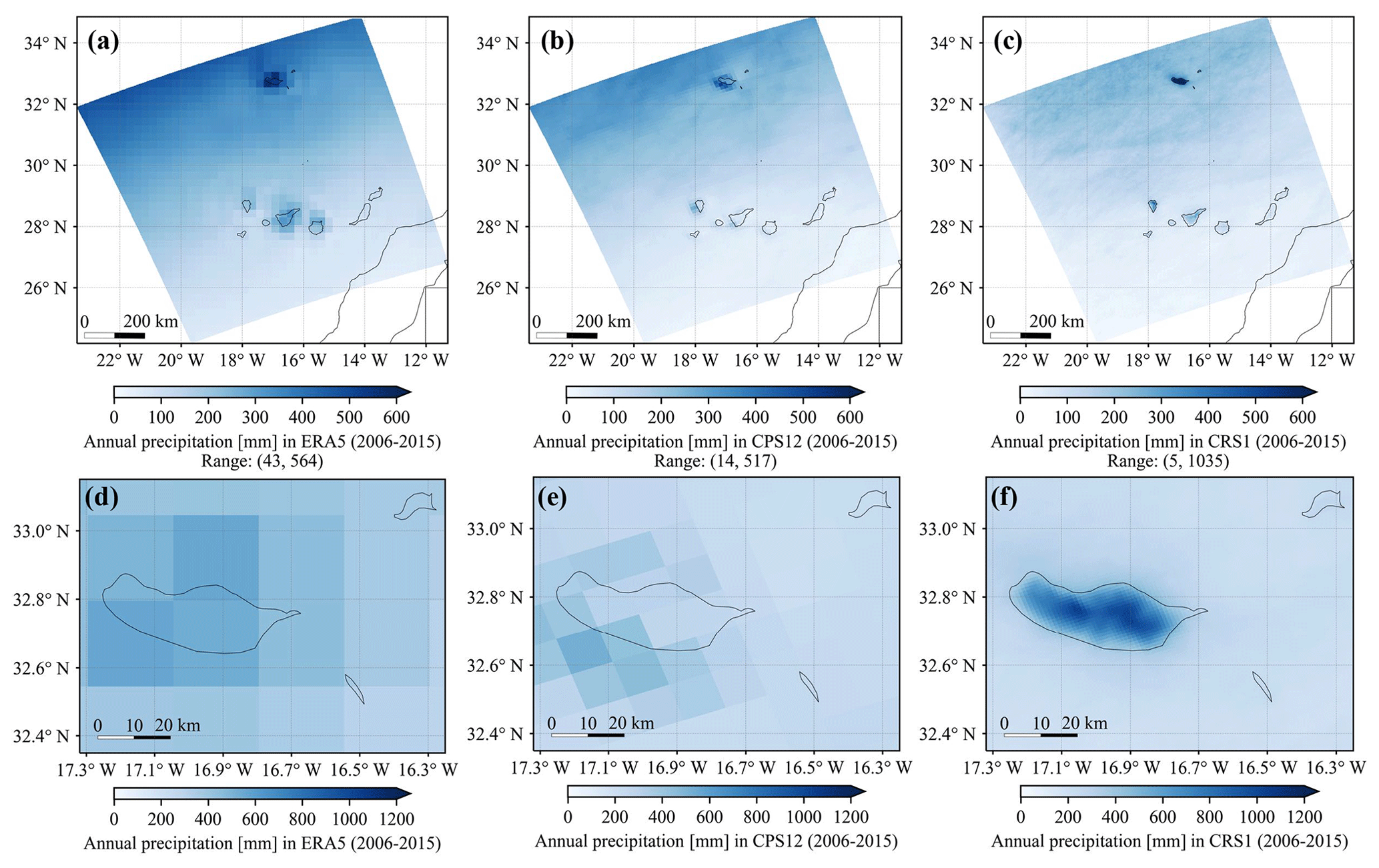
Figure 3Evaluation of precipitation [mm] against conventional surface stations. Annual-mean precipitation amounts (2006–2015) from (a) the observational dataset, (b) CPS12 and (c) CRS1. Relative biases [%] of (d) CPS12 and (e) CRS1 with respect to observations at stations. The geographic map is from the GADM (Global Administrative Areas) database.

Figure 4Monthly precipitation [mm] over Madeira Island in the ERA5 reanalysis, CPS12 and CRS1 from 2006 to 2015. For each dataset, the grid cells whose centres are located within ellipse e1 in Fig. 2a were used to calculate the spatially averaged monthly precipitation. That is, 1 grid cell (∼961 km2) in the ERA5 reanalysis, 6 grid cells (∼864 km2) in CPS12 and 666 grid cells (∼800 km2) in CRS1 were adopted.
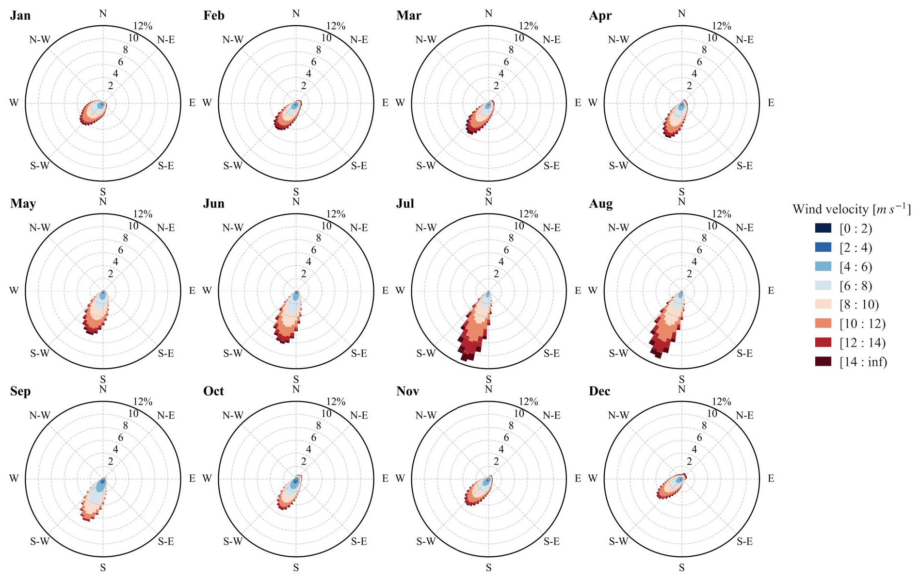
Figure 5Simulated monthly 100 m wind climatologies for 2006–2015 in CRS1 over the analysis region defined in Fig. 2a based on hourly data in CRS1. The wind roses can be understood as histograms of wind direction that simultaneously take into account wind velocity varying from 0 to more than 14 m s−1. Each sector with a width of 5∘ points in the direction of the wind, and its radius represents the frequency.

Figure 6(a) Monthly climatology of inversion height and (b) diurnal cycle of inversion height. Both panels show monthly/hourly means and standard deviations (SDs). The observed values were calculated from the Funchal radiosonde data from IGRA 2, and the simulated values near Funchal were calculated based on the model simulation CRS1 at the grid point closest to the Funchal radiosonde station. The simulated values over se were used to represent upstream conditions where decadal 3D model outputs are available. The altitude of two mountain peaks, Pico Ruivo (1862 m) and Paul da Serra (1500 m) at Madeira Island, are indicated for reference.

Figure 7Synoptic-flow conditions including mean sea level pressure and 10 m winds from the ERA5 reanalysis at the (a) starting, (b) middle and (c) ending time of the case study period. A wind velocity of 10 m s−1 is shown for reference. H (L) represents high-pressure (low-pressure) systems. The geographic map is from Natural Earth.
The 100 m wind climatology in CRS1 during 2006–2015 over the analysis region defined in Fig. 2a is shown in Fig. 5. Equivalent plots with data from the ERA5 reanalysis (not shown) have quite similar monthly patterns and indicate good performance of our simulation in terms of wind climatology. Our analysis region is dominated by northeasterlies throughout the year, consistent with trade winds. A significant concentration in wind direction and an increase in mean wind speed from April to August generate favourable conditions for vortex shedding as shown in Sect. 3.3.
In Fig. 6a, the monthly inversion height observed at the Funchal radiosonde station from 2006 to 2015 also shows very interesting patterns. Firstly, the observed monthly mean inversion height decreases from about 1.5 km in April to around 1 km in July and August, which is conducive to flow splitting and thus vortex shedding. It then increases to above 1.6 km in September and results in unfavourable conditions for vortex shedding, like the winds in Fig. 5, both of which are influenced by the Azores high-pressure system. The observed monthly mean inversion height is about 1.5 km from September to April. By comparing the monthly inversion height in observations and simulations in CRS1, we can detect that their standard deviations are rather close and the monthly patterns are very well simulated despite consistent negative biases of around 150 m. As atmospheric conditions at Funchal are disturbed by Madeira Island, we also show the monthly inversion height in CRS1 over the ellipse se from Fig. 1b with upstream conditions under prevailing northeasterlies. Unfortunately, the flow in se is still strongly affected by the orography and therefore does not represent undisturbed upstream conditions (which we lack due to the limited domain with 3D data). However, using it still gives us some indications about the variability in the inversion height. The simulated values over se are close to those near Funchal except in July and August, where the monthly mean inversion height is lower at Funchal, possibly due to downslope winds (Durran, 1990) resulting from strong northeasterlies as shown in Fig. 5. Typical vertical temperature profiles from the radiosonde observations and the simulation are given in Fig. C2. The simulated and observed inversion height in this example agrees relatively well but shows the same bias as in Fig. 6a.
The simulation data for Fig. 6a were extracted using the same timestamps as the Funchal radiosonde observations with 98.4 % of the observations being conducted at 12:00 UTC. Consequently, we present the diurnal cycle of inversion height in Fig. 6b to examine the representativeness of the data at 12:00 UTC. The model outputs near Funchal show a clear diurnal cycle. The hourly mean inversion height exceeds 1250 m from 12:00 to 17:00 UTC and lies below 1150 m from 21:00 to 08:00 UTC. Such a diurnal cycle can also be observed for each calendar month (not shown). Hence, the observations and simulations near Funchal primarily at 12:00 UTC in Fig. 6a are representative even though the 12:00 UTC data exhibit around 80 m higher inversion height than the daily mean. As the simulated values over ellipse se in Fig. 6b display nearly no diurnal cycle, the simulated values over ellipse se in Fig. 6a are also quite representative. The inversion height estimated with the Tenerife radiosonde observations at 28.32∘ N, 16.38∘ W reveals similar monthly patterns and negative biases in simulations as in Fig. 6a and is generally lower than that at Funchal (not shown).
3.2 Case study of 3–9 August 2010
To investigate the characteristics of vortex streets, we selected a vortex-shedding event that lasted for about 1 week from 3 August 2010 at 20:00 UTC to 9 August 2010 at 07:00 UTC. The animation of simulated 100 m wind velocity and direction during this period can be found in “Video supplement” V1 (video 1) (Gao et al., 2021). The average upstream wind velocity is around 12 m s−1. We can see that winds are accelerated at the island flanks and decelerated before and behind Madeira Island, which indicates horizontal flow splitting. The corresponding animation of derived 100 m relative vorticity is shown in “Video supplement” V2 (Gao et al., 2021), which acts as a good tracer for vortex streets and shows some variations during this event. Snapshots of this vortex-shedding event can be found in Figs. 9 and 11. In animation V2, lime contours encompass 347 identified vortices using our vortex identification algorithm described in Sect. 2.4. For this case study, the vortex detection methodology was checked manually. Of all identified vortices, 344 were identified correctly, and 3 were wrongly identified and highlighted in cyan in animation V2. This corresponds to a false-positivity rate (FPR) (Yang et al., 2020) of 0.9 % and one falsely identified vortex every 44 h. Occasionally, stratocumulus clouds can also serve as tracers for vortex streets, so we visualised cloud patterns during this period in “Video supplement” V3 (Gao et al., 2021) using the high-rate SEVIRI rectified image data of Meteosat-9 in MSG from EUMETSAT (Schmetz et al., 2002). Although cloud patterns are not as indicative as relative vorticity for the detection of vortex streets, we can still observe a well-organised vortex-shedding event in animation V3 that agrees well with the simulations.
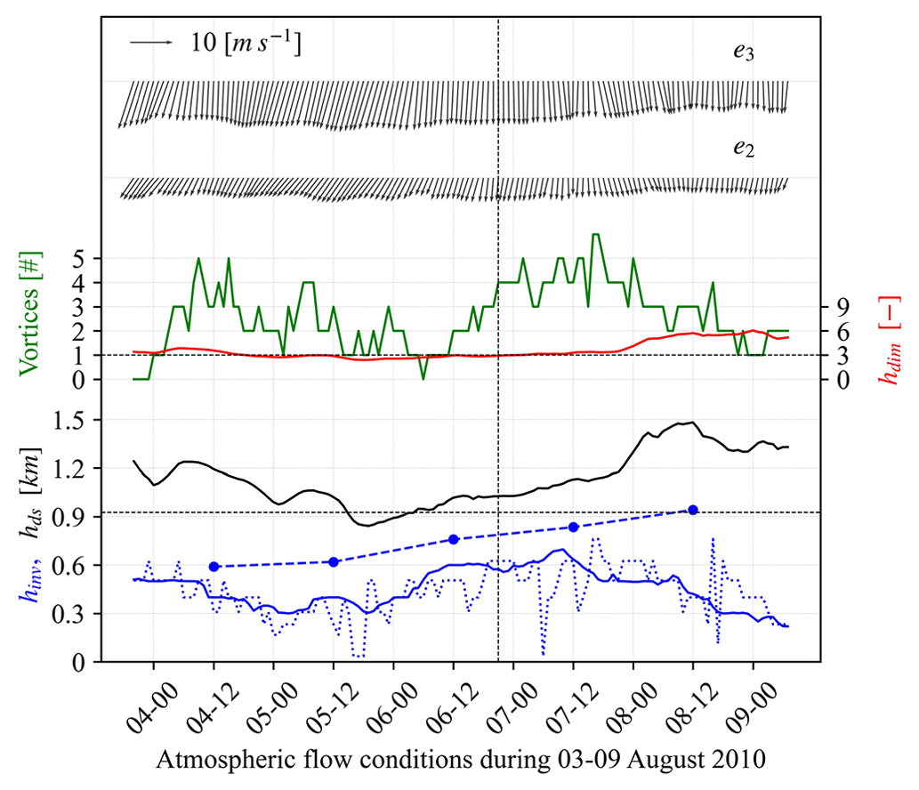
Figure 8Local flow conditions during the case study period (from 3 August 2010 at 20:00 UTC to 9 August 2010 at 07:00 UTC). The top two rows of arrows represent average wind arrows over ellipses e3 and e2, and a wind velocity of 10 m s−1 is shown for reference. The third row shows the number of identified vortices (green line), and the average dimensionless mountain height hdim over e3 (red line). The dividing streamline height hds over e3 is shown as the black line. The solid blue line represents the inversion height hinv over e3, and dashed and dotted blue lines show hinv in Funchal radiosonde observations and CRS1 in a grid cell closest to the Funchal radiosonde station, respectively. A selected timestamp of 6 August 2010 at 21:00 UTC for subsequent analysis is indicated by a vertical dashed black line.
Figure 8 demonstrates time series of local flow conditions around Madeira Island during this period. The uppermost array of arrows represents the mean 100 m wind direction and velocity averaged over ellipse e3 in Fig. 2a, which can be assumed to be undisturbed flow conditions. Wind velocity in e3 generally exceeds 10 m s−1 with only slightly varying wind direction. Winds over e2 are much weaker and significantly dispersed, so we used undisturbed flow conditions from e3 for subsequent analysis. The green line in Fig. 8 shows the number of correctly identified vortices shed from Madeira Island, which shows large variations during this period. The dimensionless mountain height hdim averaged over e3 shown in the red line is generally above 3, a value that Schär and Durran (1997) used to specify flow conditions favourable for vortex shedding. The dividing streamline height hds mostly exceeds 60 % of the peak mountain height in CRS1 (∼0.93 km denoted with a dotted black line), which is a widely used threshold to distinguish flow conditions conducive for vortex shedding. The weak vortex-shedding signals at the middle of this period seem to coincide with stages where hds and hdim fall below the corresponding thresholds. The comparison of inversion height from Funchal radiosonde observations at 12:00 UTC and a grid cell in CRS1 closest to Funchal radiosonde station in the dashed and dotted blue lines shows expected patterns as described in Sect. 3.1: negative bias and vulnerability to perturbations in lower levels in the simulations.
Synoptic-flow conditions including mean sea level pressure and 10 m winds from the ERA5 reanalysis during this period are shown in Fig. 7. At the beginning of this period, a high-pressure system centred north of the Azores resulted in a strong northeasterly flow, especially over the northwest of our study domain. Subsequently, the high-pressure system moved northeast and deformed towards a circle, which was associated with well-organised vortex streets in the lee of Madeira Island, whose major axis is approximately perpendicular to the mesoscale wind direction. At the end of this event, the vortex-shedding phenomenon weakened with the weakening of the high-pressure system. Consequently, we can identify a clear correlation between vortex shedding in the lee of Madeira Island and the high-pressure system, which is well known as the semipermanent Azores high (Davis et al., 1997) and forms one pole of the North Atlantic Oscillation (NAO) (Visbeck et al., 2001).
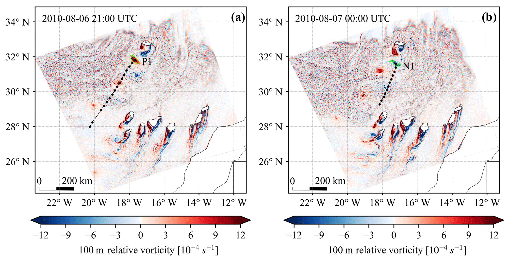
Figure 9Relative vorticity at 100 m and tracks of (a) a positive vortex P1 shed on 6 August 2010 at 21:00 UTC and (b) a negative vortex N1 shed on 7 August 2010 at 00:00 UTC. The relevant vortices are encompassed by lime contours, and the tracks in the next hours are shown with black lines and dots on an hourly basis. A gap in the lower half of the track of P1 results from a false rejection of that vortex by our algorithm. The geographic map is from Natural Earth.
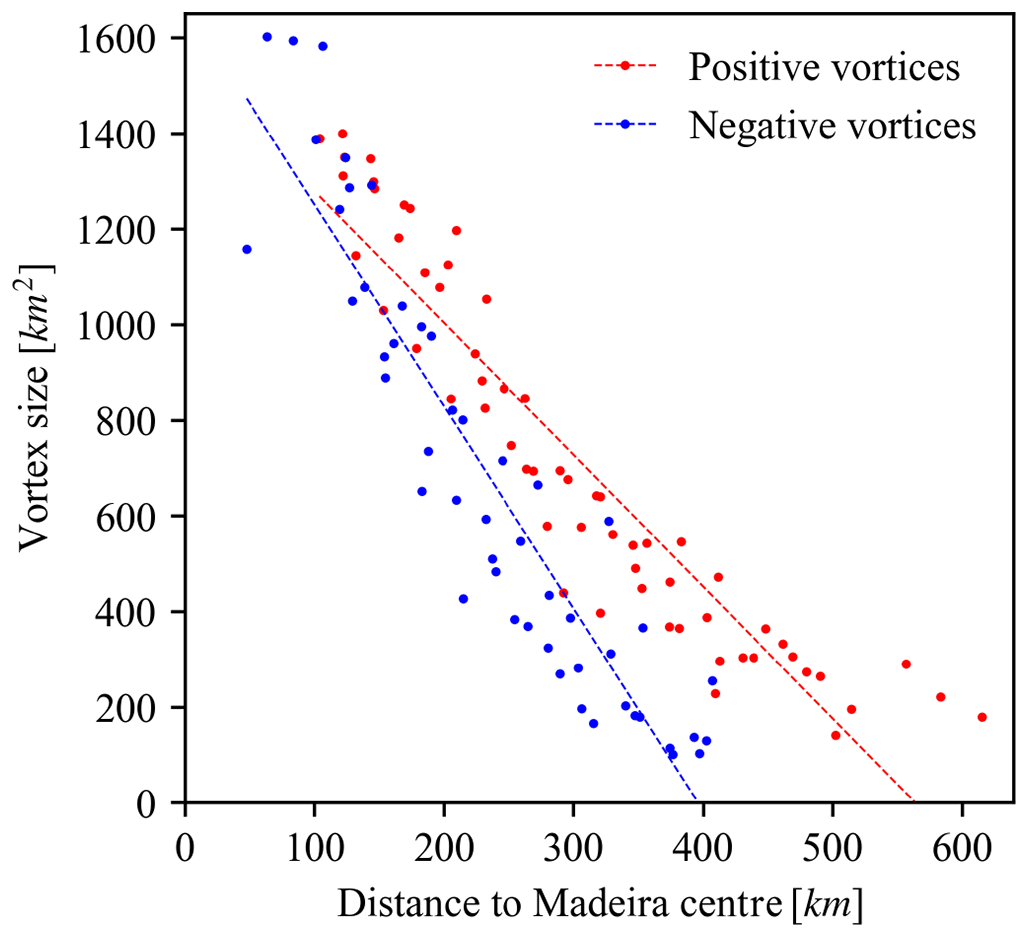
Figure 10The size of four positive and four negative tracked vortices (see “Video supplement” V4, Gao et al., 2021) against their distance to the Madeira centre. Two dashed lines are fitted to the scatterplots to show different decaying rates of positive and negative vortices.
We manually tracked four positive vortices labelled as P1 to P4 and four negative vortices (N1–N4) starting from the selected timestamp. Tracks of P1 and N1 are shown in Fig. 9, and the animation of their propagation can be found in “Video supplement” V4 (Gao et al., 2021). Based on the eight vortices, we calculated several key numbers to compare with existing literature and satellite images. The ratio of advection velocity of vortices to undisturbed wind velocity over e3 has a mean of 0.82 and a standard deviation of 0.02, while existing literature reported a large range of values like 0.76 in Tsuchiya (1969) or 0.90 ± 0.37 in Heinze et al. (2012). The average shedding interval of like-rotating vortices is about 6.7 h, and a rough estimation based on satellite images in this period gives a value of around 7 h. The corresponding Strouhal number has a mean of 0.154 and varies from 0.142 to 0.166, which also lies in or close to the reported range from Nunalee and Basu (2014) of between 0.15 and 0.22. Figure 10 presents the size of eight tracked vortices from 100 to 1600 km2 against their distance to the Madeira centre up to 600 km. We can see a faster decay of negative vortices, which might be attributed to the Coriolis force, as the Rossby number defined in Eq. (5) has a value of around 4 considering a relevant length scale of L=35 km, a flow velocity of u=10 m s−1 and a latitude of ϕ=32deg.
For the decade-long simulations, only a reduced set of output fields was stored. To investigate the simulated vortex streets in detail, we restarted the model simulation on 1 August 2010 at 00:00 UTC for the case study period to generate variables every 100 m in the lowest 5 km above the surface. Figure 11 shows the 100 m relative vorticity, 10 m potential temperature and 100 m specific humidity at the selected timestamp in the new model simulation. Small differences can be found between Figs. 11a and 9a due to stochastic properties of simulations. We can identify positive potential temperature anomalies at 10 m altitude as mentioned in Sect. 2.4 and positive specific humidity anomalies around both positive and negative vortices. Both kinds of anomalies were observed in the wake of Hawai'i (Smith and Grubišić, 1993). The potential temperature anomalies result mainly from temperature anomalies and could be used as a tracer for vortex streets in idealised simulations (Heinze et al., 2012).
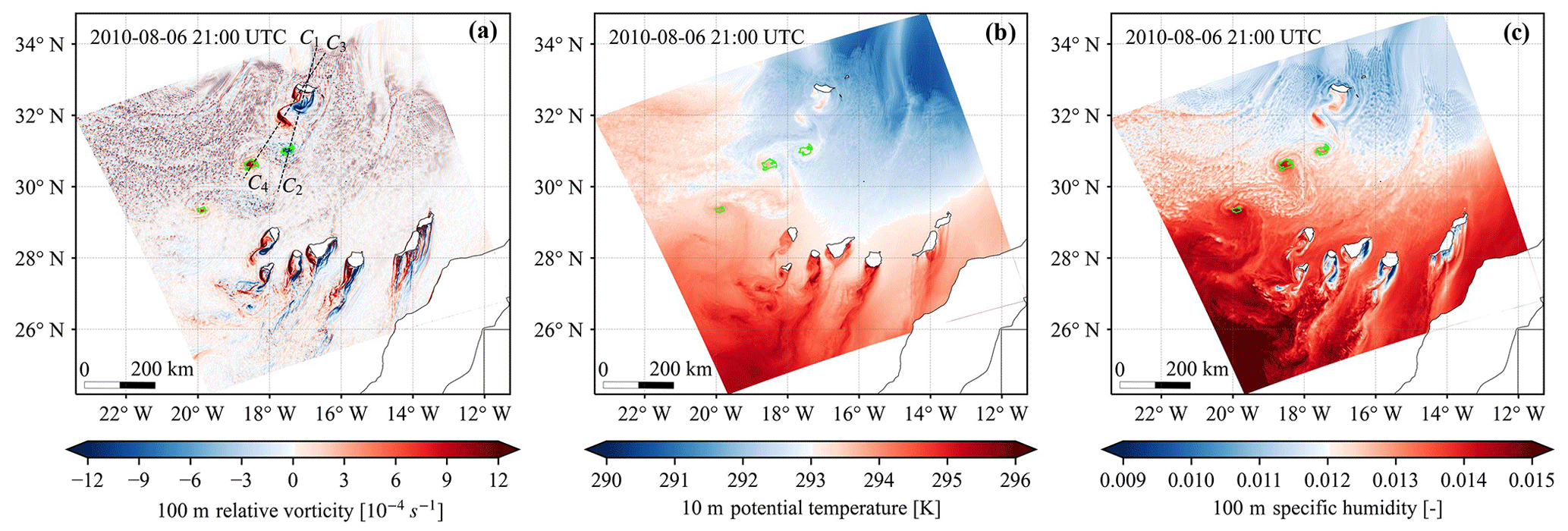
Figure 11The (a) 100 m relative vorticity, (b) 10 m potential temperature and (c) 100 m specific humidity on 6 August 2010 at 21:00 UTC. The vertical structures of the vortices were investigated along two cross-sections (C1–C2 and C3–C4) shown in (a). The identified vortices are encompassed by lime contours. The geographic map is from Natural Earth.
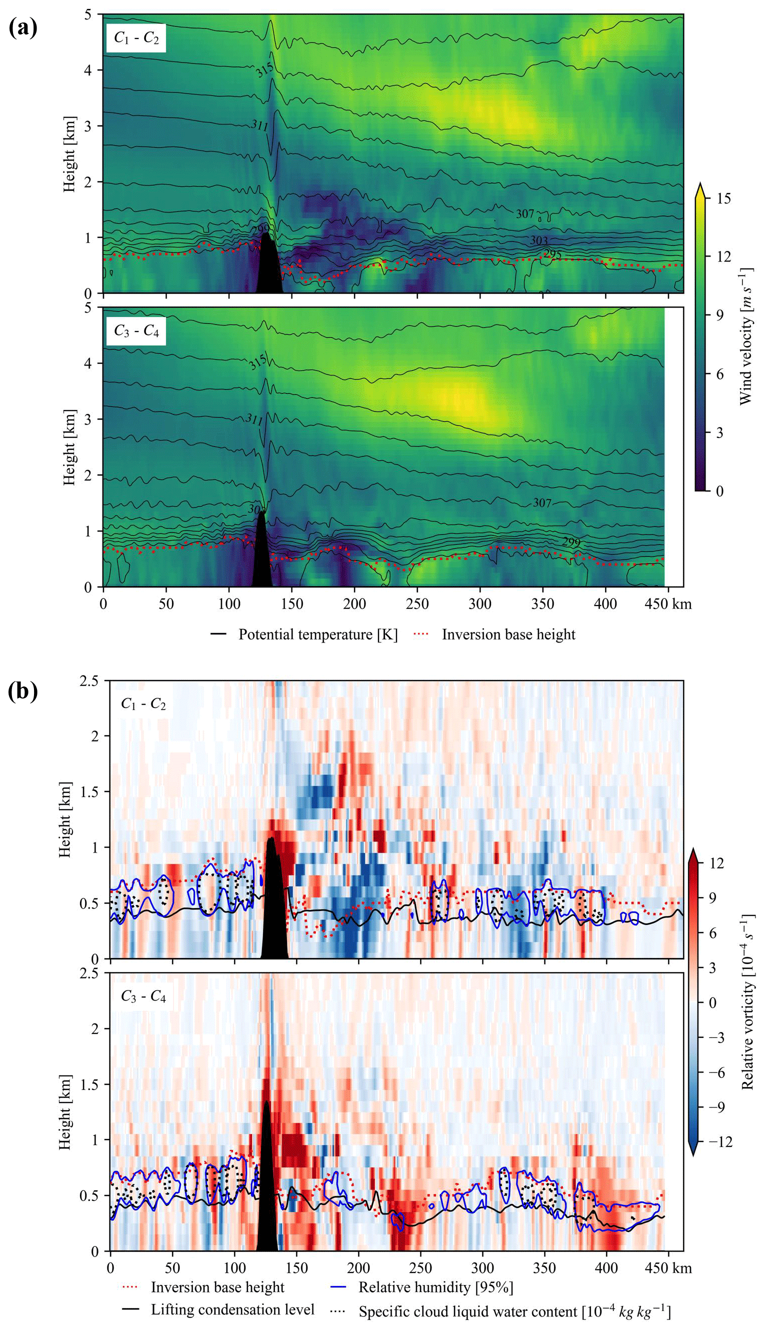
Figure 12Vertical structure of (a) wind velocity, potential temperature and inversion base height and (b) relative vorticity, relative humidity, lifting condensation level and specific cloud liquid water content along cross-sections C1–C2 and C3–C4 shown in Fig. 11a on 6 August 2010 at 21:00 UTC.
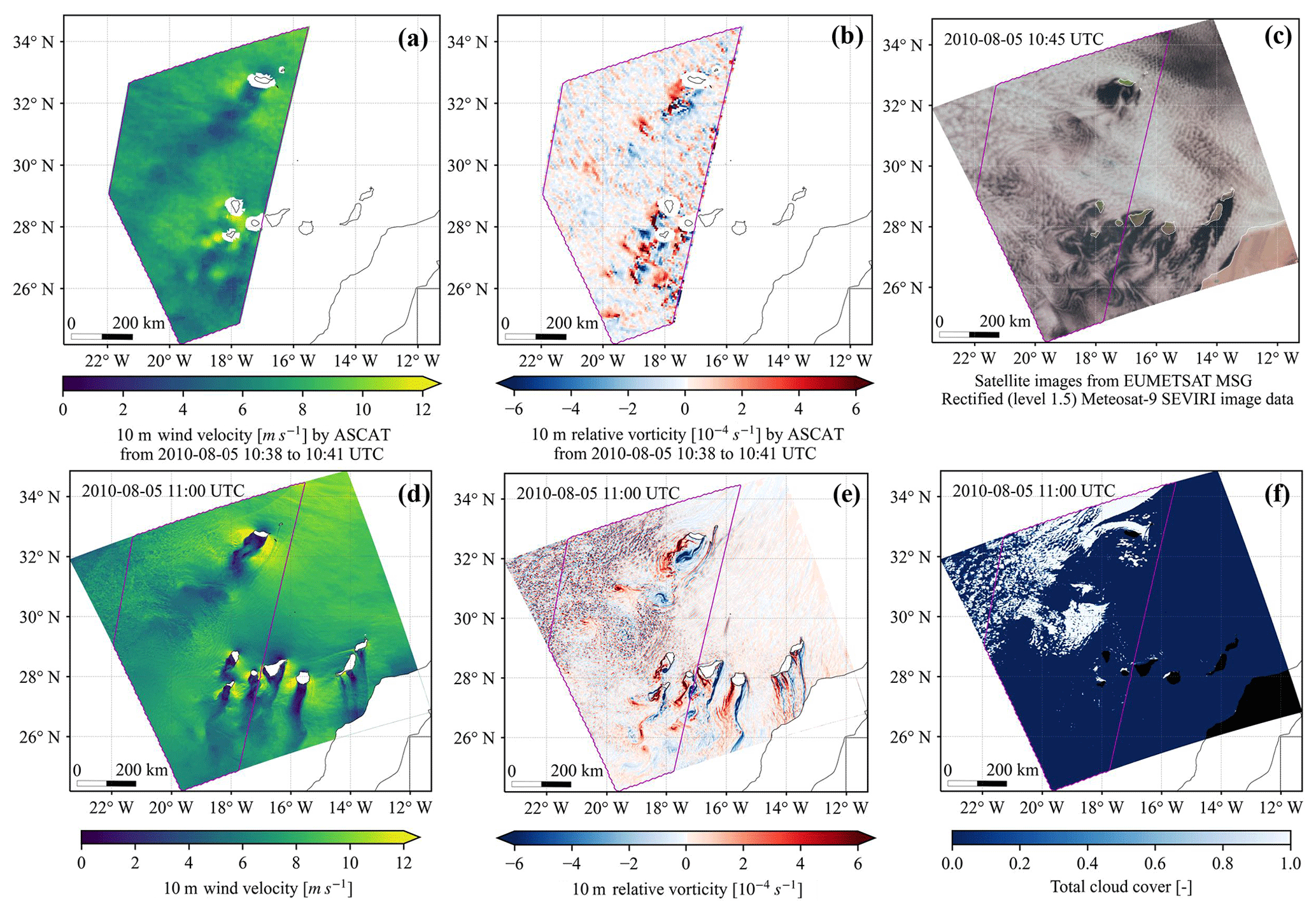
Figure 13Comparison of (a–c) satellite data versus (d–f) simulation data: (a) 10 m winds and (b) the derived relative vorticity at a horizontal resolution of 6.25 km measured by ASCAT on board Metop-A from EUMETSAT. The magenta polygons indicate the area with available ASCAT data over the analysis region. (c) Satellite image constructed with data observed by MSG Meteosat-9 from EUMETSAT. The NIR1.6, VIS0.8 and VIS0.6 channel data were used to represent red, green and blue. The second row shows (d) 10 m winds, (e) the derived relative vorticity and (f) total cloud cover in CRS1 at a time point (5 August 2010 at 11:00 UTC) close to that of observations. The geographic map is from Natural Earth.
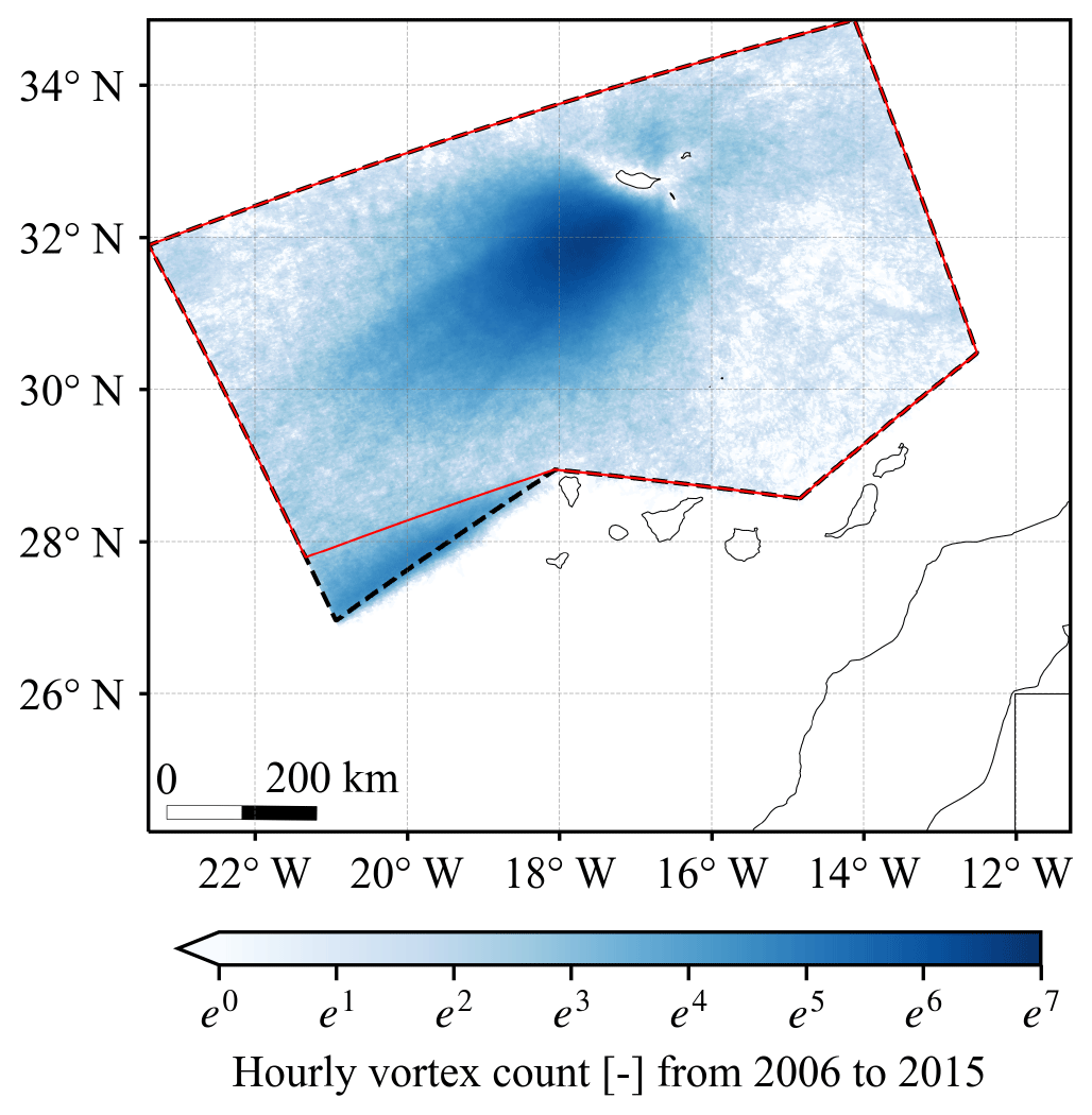
Figure 14Hourly vortex count at each grid cell in CRS1 from 2006 to 2015 (in total 87 648 h, e7≈1097). It shows the results when we used the dashed black polygon to restrict the region where the centre of vortices shed from Madeira Island can appear as described in Sect. 2.4. For each grid cell at each hour, we counted the vortex number as one if an identified vortex covers this grid cell. The exponential scale was used to account for the unevenly distributed frequency in vortices. The geographic map is from Natural Earth.
The vertical structures of vortex streets along cross-sections C1–C2 and C3–C4 depicted in Fig. 11a are shown in Fig. 12. The two cross-sections show similar signals. From Fig. 12a we can observe a well-mixed upstream boundary layer, gravity waves above the island, distorted downstream isentropes, a lowering of the downstream capping inversion and six downstream positive potential temperature anomalies extending from the surface to the inversion height. The last potential temperature anomaly from C1 to C2 has no corresponding vortex, which indicates that vortex streets can still impact the atmosphere further downstream even though the vortices already dissipated. The lifting condensation level (LCL) is the height where an air parcel would saturate when lifted adiabatically. Although the LCL is estimated based on surface data (Romps, 2017), it well captures the lower bounds of contours of 95 % relative humidity. The cloud-free region in the lee of Madeira Island in the animation V3 in “Video supplement” (Gao et al., 2021) can be explained by the lowering of the inversion base below the LCL and can result in intense solar radiation and thus a warm oceanic wake (Azevedo et al., 2020). In satellite images, we could sometimes observe cloud-free conditions (eyes) in the centre of shed vortices. The inversion base lower than LCL was assumed to be responsible for cloud-free eyes of vortices (Heinze et al., 2012), but this is not supported by our simulation as the inversion base is higher than LCL at downstream vortices.
It is still difficult to validate the track and timing of individual vortices in realistic simulations because of limited observations. During our case study period, vortex streets in the lee of Madeira Island were captured in only three snapshots by ASCAT on board the Metop-A satellite, of which the clearest one from around 5 August 2010 at 10:40 UTC is shown in Fig. 13a and b. The 10 m relative vorticity derived from the observed wind vectors shows distinct vortex-shedding signals which coincide with cloud patterns observed by Meteosat-9 in Fig. 13c. The corresponding model outputs on 5 August 2010 at 11:00 UTC in Fig. 13d and e also show obvious vortex streets in the lee of Madeira Island, which agrees well with the observations. Note also that we cannot expect a perfect spatial fit as vortex shedding is a chaotic phenomenon and the timing is long in a simulation such as ours. The simulated cloud patterns in Fig. 13f do not agree with the observations, and it looks like the model has difficulties in the simulation of clouds for this specific situation. This is not uncommon, as the simulation of clouds is still a big challenge even in high-resolution weather and climate models (Bretherton, 2015), and the dynamics of stratocumulus clouds are particularly hard to resolve (Schneider et al., 2019).
For further justification of our vortex identification algorithm, relevant vortex statistics are presented in Appendix B.
3.3 Climatology of Madeira vortex streets
In this section, we present the decadal analysis of vortex streets in the lee of Madeira Island. For the case study in Sect. 3.2, we required the centre of vortices shed from Madeira Island to be within the black dashed polygon in Fig. 14 to incorporate as many vortices as possible. For the decadal analysis, we chose a smaller domain, shown by the red polygon in Fig. 14, to exclude vortices shed from the La Palma Island in the Canary Archipelago. The vortex count shown in Fig. 14 shows a strongly increased frequency to the southwest of Madeira Island, which corresponds to the lee during trade wind conditions.
Figure 15a shows the daily vortex count during 2010 and the 10 d moving average. As the parameters of our algorithm were tuned based on data from February and August 2010, we validated it using data from November 2010 against a manual analysis of the simulated vorticity field. During this month, there are 199 identified vortices and 171 correctly identified vortices, which correspond to a false positive rate (FPR) of 14 % and one falsely identified vortex every 26 h. Although this FPR does not suggest as good a performance as 0.9 % in the case study in Sect. 3.2, the second index still provides confidence in our algorithm. Figure 15b shows the monthly vortex count from 2006 to 2015, and the corresponding boxplots are shown in Fig. 16, where several interesting phenomena can be observed. While Fig. 16a shows distinct inter-annual variations, Fig. 16b indicates a large monthly discrepancy. An increasing vortex-shedding rate can be observed from April to August in Fig. 16b, as the wind direction is increasingly concentrated and the mean wind speed is increased in Fig. 5, while the inversion height decreases from around 1.5 to 1 km in Fig. 6a. There are large variations and occasionally strong vortex-shedding signals in March, which might result from abnormally lower inversion base in Fig. 6a and less precipitation in Fig. 4. Furthermore, we can see a sharp transition from August to September resulting from a sudden deceleration of winds in Fig. 5 and the increase in inversion height in Fig. 6a. This transition is also found in the study of Grubišić et al. (2015) by manually checking 8 years of satellite images.
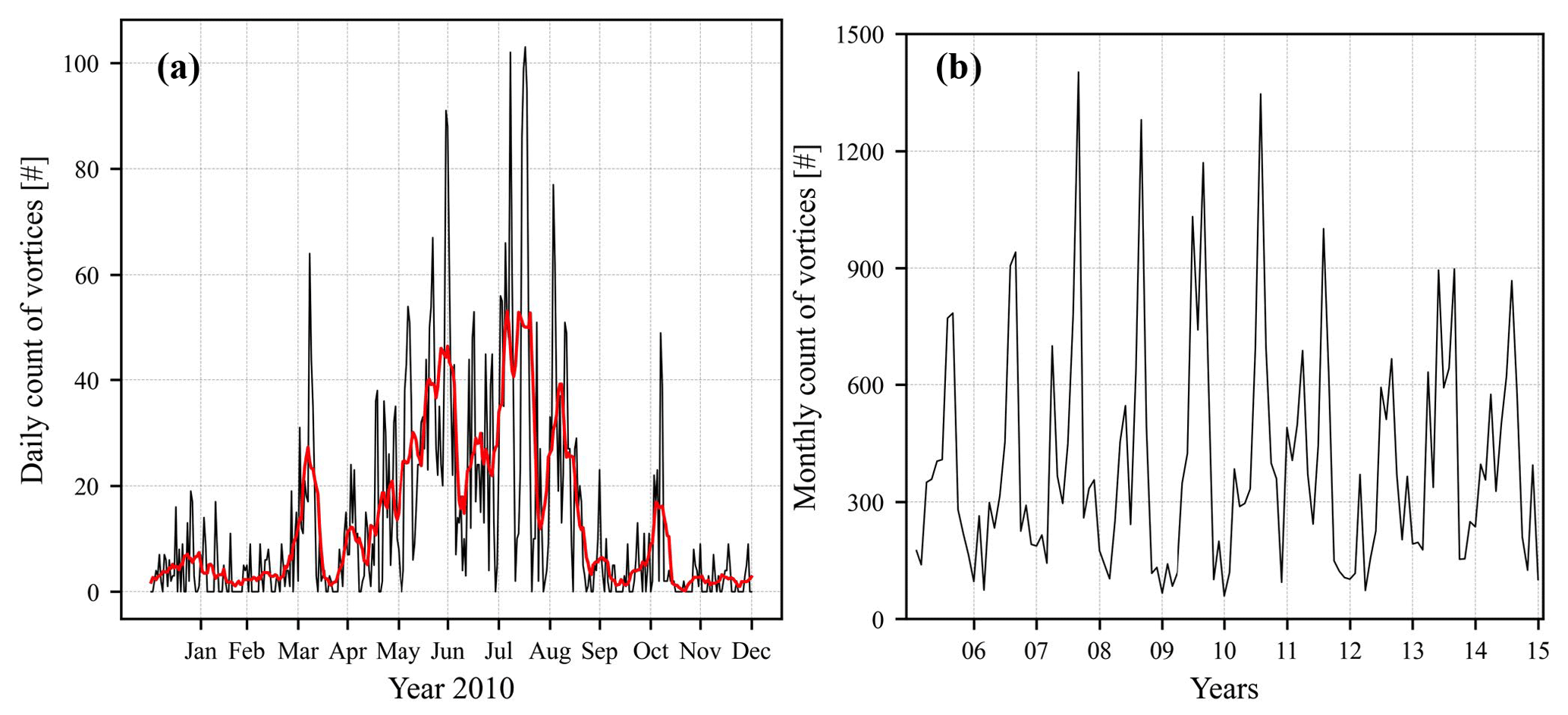
Figure 15(a) Daily count of identified vortices in CRS1 in 2010 in black and its 10 d moving average in red. (b) Monthly count of identified vortices in CRS1 from 2006 to 2015.

Figure 16Boxplot of the monthly count of identified vortices in CRS1 from 2006 to 2015 in (a) each year and (b) each month. The boxes show quartiles of the data, and the whiskers extend to values within 1.5 times of the inter-quartile range from the low or high quartiles.
This study investigated vortex streets in the lee of Madeira Island during 2006–2015. We used the regional climate model COSMO with a horizontal grid spacing of 1.1 km, driven by the ERA-Interim reanalysis. Firstly, we explored meteorological conditions over our study area using the ERA5 reanalysis, model simulations and radiosonde observations. Then we studied the basic properties of vortex streets based on a case study during 3–9 August 2010 and developed a vortex identification algorithm. This algorithm was subsequently used for the climatological analysis of vortex streets over a 10-year period.
Although there are some discrepancies between simulated and observed precipitation, the added value of high-resolution simulations that partly resolves the complex topography and convective processes is rather prominent. In particular, the CRS1 simulation shows more realistic spatial patterns and less negative biases over Madeira Island than the CPS12 simulation with 12 km horizontal grid spacing. The monthly wind conditions over our analysis region can be well simulated and reveal some interesting phenomena. From April to August, the trade wind speed increases and the direction becomes better defined. Between August and September, the trades become much weaker again. In addition, the monthly patterns of inversion height obtained from radiosonde observations at Funchal are also well captured in CRS1. From April to August the inversion height decreases from 1.5 to 1 km, whereas it increases abruptly to above 1.6 km in September. Such monthly patterns of winds and inversion height can be explained by the migration of the Hadley cell (Carrillo et al., 2016) and associated shifts in the Azores high.
A vortex-shedding event behind Madeira Island during 3–9 August 2010 observed by Meteosat-9 of EUMETSAT is well captured by CRS1. This event was chosen as a case study to investigate and validate the basic properties of vortex streets in realistic simulations. During this period, both synoptic and local atmospheric conditions were found to be conducive to vortex shedding. The synoptic-flow conditions from the ERA5 reanalysis reveal a direct dependence of vortex shedding in the lee of Madeira Island on the location, shape and magnitude of the Azores high. The upstream undisturbed 100 m winds have a velocity over 10 m s−1 and show small spatial and temporal variations. In addition, both the dimensionless mountain height and the dividing streamline height satisfy widely studied requirements for flow splitting and vortex shedding. Overall, the numerical model indicates good performance in realistically simulating vortex shedding in this region and reveals interesting properties of vortex streets. Firstly, the ratio of advection velocity of vortices to undisturbed wind velocity over e3 was estimated to be around 0.82, and the Strouhal number varies between 0.142 and 0.166, both values lying well within reported ranges in the literature. It is found that the negative vortices show faster decay rates than positive vortices. A potentially attractive explanation is related to the role of the Coriolis force, which sharpens positive (cyclonic) vortices and weakens negative (anticyclonic) ones. The investigation of structures of vortex streets in realistic atmospheric simulations brought us several new insights. Although positive potential temperature and specific humidity anomalies around vortices are well known for many vortex streets, the fact that they can propagate further downstream than the dynamical (vorticity) contribution of the vortices has not yet been widely noticed. Finally, the lowering of the capping inversion below the LCL is responsible for cloud-free regions in the lee of Madeira Island.
Based on the case study, we developed a rule-based vortex identification algorithm. The algorithm was manually validated and shows a good performance with few wrong identifications. This algorithm enabled us to draw a 10-year climatology of vortex shedding to the lee of Madeira. Monthly patterns of the number of identified vortices shed from Madeira Island are consistent with that of winds over our analysis region and the inversion height observed at Funchal. These patterns are mainly governed by the annual cycle of the trades, Hadley circulation and the Azores high. From April to August, the vortex-shedding rate is increasing. This is driven by a strengthening of the trade winds and a lowering of the inversion height. Thereafter, the sudden weakening of the trade winds and an increase in inversion height in September lead to a pronounced and sharp drop in vortex-shedding frequency, confirming the results of Grubišić et al. (2015) obtained from 8 years of satellite images.
Lastly, we point out some limitations in our work and make several suggestions for future studies. Although the islands in the Canary Archipelago, especially La Palma and El Hierro, also show very nice vortex-shedding signals, we do not consider multiple islands in one paper for simplicity and feasibility. While we used the 6-hourly ERA-Interim reanalysis as initial and boundary conditions for CPS12, the employment of the ERA5 reanalysis with higher spatial and temporal resolution might improve the simulation of vortex streets. Although our work involved only 2D vortex identification, our algorithms can be extended for 3D vortex identification. The 3D vortex visualisation, automatic vortex tracking and vortex identification using deep learning could also be considered in further works. The kinematic vorticity number could also be considered for vortex identification in future work (Schielicke et al., 2016). Finally, we noted some considerable challenges such as limitations in the simulation of the cloud cover in particular in areas of stratocumulus. Nevertheless, we believe that our model-based generation of a vortex-shedding climatology is overall successful.
Abramovich et al. (2000) focused on statistical applications of the wavelet analysis and could serve as a good starting point for statisticians. All wavelets in the basis are derived from two mutually orthonormal parent wavelets through translations of the scaling function ϕ and dilations and translations of the mother wavelet ψ as
where j0∈Z is fixed; Z is the set of integers; k∈Z; and .
Intuitively we can regard ϕ as a kernel function and ψ as a localised oscillation, where a unit increase in j in Eq. (A2) doubles the frequency or resolution of ψjk(t). A unit increase in k shifts the location of by and ψjk(t) by 2−j.
Given a wavelet basis and assuming a signal to be infinite, g(t) can be represented through a wavelet series as
where and .
Considering discretely sampled signals (assume n=2J, where J is a positive integer) at a constant interval, the DWT (discrete wavelet transform) needs to be considered
where W is an n×n orthogonal matrix associated with selected wavelets and d is an n×1 vector comprising discrete scaling coefficients (, ) and discrete wavelet coefficients djk (, , ).
The inverse DWT can be obtained based on the orthogonality of W as g=WTd and used to denoise through reserving only a part of the largest values in d (Wickerhauser, 1996; Ruppert-Felsot et al., 2005), where coefficients above (below) a threshold are assumed to correspond to signals (noise). The choice of the threshold depends on a measure of the number of significant coefficients N0 defined as
where H(g) is the entropy of g and defined as
where and .
As for the selection of parent wavelets, the function support (compact or infinite), orthogonality, smoothness (i.e. regularity or the number of continuous derivatives) and the number of vanishing moments should be considered. Wang et al. (2018) give a good visualised introduction to wavelet families, while some recommendations and requirements about their selection can be found in Domingues et al. (2005) and Jawerth and Sweldens (1994). The Haar basis is the oldest and simplest wavelet basis for g(t). Although the Haar basis does not have a good time–frequency localisation and the resulting wavelets are discontinuous and thus unsuitable for smooth functions, its performance was equivalent to other wavelets in our preliminary analysis, as also reported by Siegel and Weiss (1997). Therefore, it is selected for our further analysis for simplicity. In real cases, signals are normally zero outside a finite interval. As simply setting the signals to be zero outside the finite interval results in discontinuities at boundaries, periodic boundary handling is adopted as a solution.
In Fig. B1, we display several properties of extracted vortices using the first two steps of our vortex identification algorithm, identified vortices through subsequent criteria and three falsely identified vortices during the case study period. Figure B1a shows that the mean relative vorticity of identified vortices distributes well above the threshold s−1 selected to identify candidate grids. Some extracted vortices have mean relative vorticity below the selected threshold. Two reasons can explain this phenomenon: these vortices have a mean size of 4 km2 and thus are vulnerable to noise; the wavelet transform could increase the relative vorticity above the threshold, whereas we extract the vortex characteristics based on the original data. We can see a sharp edge of the size of identified vortices at the threshold of 100 km2, which indicates some falsely rejected small vortices. However, we expect those small vortices to have less relevance and accept the threshold to eliminate a large number of noisy structures. Figure B1c–e reveal significant discrepancies between statistics of identified vortices and the thresholds in our algorithm. This is a great signal that indicates our algorithm consists of loose criteria and does not implicitly determine these vortex characteristics.
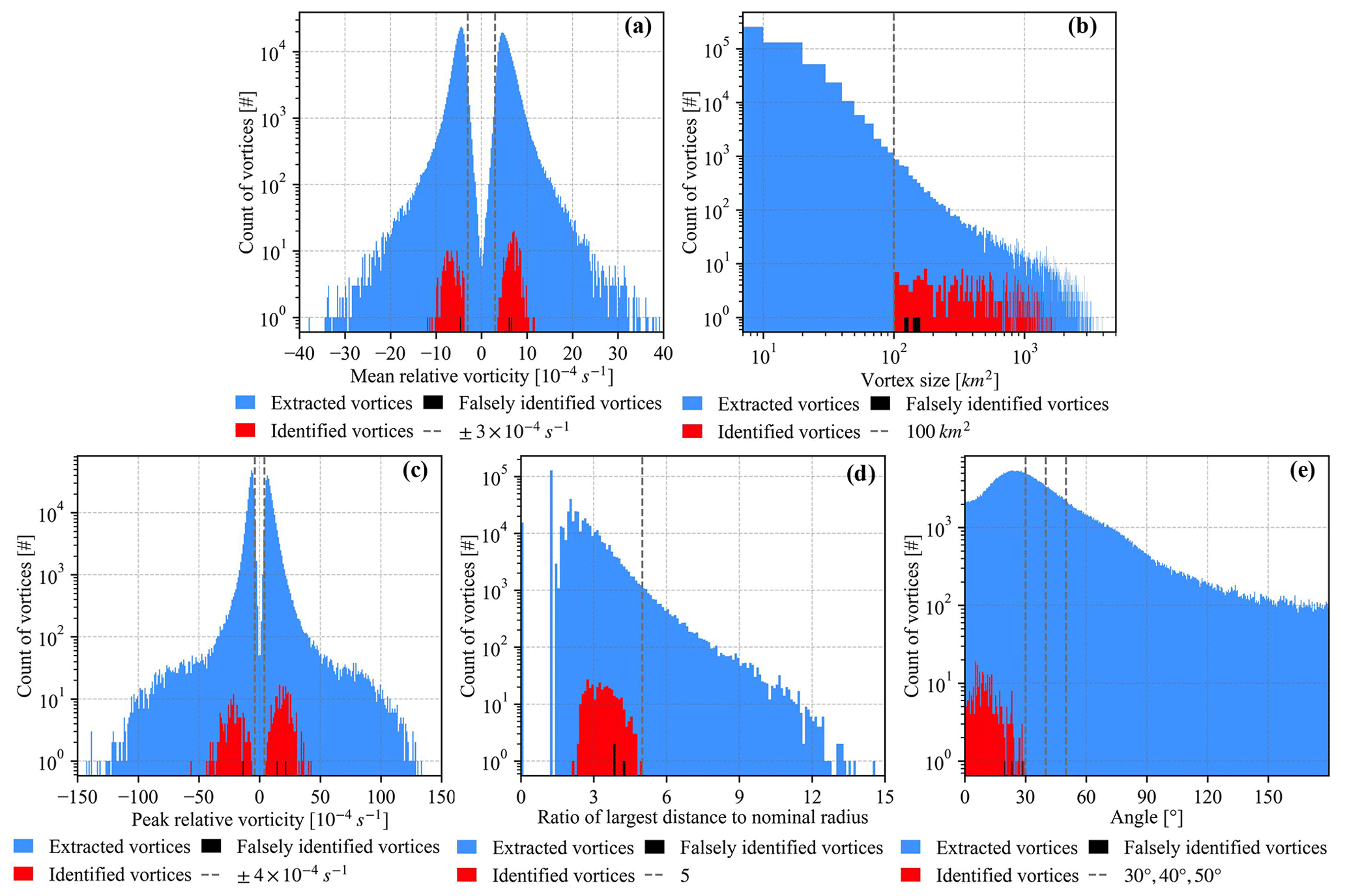
Figure B1Histograms of vortex statistics including (a) mean relative vorticity, (b) vortex size, (c) peak relative vorticity, (d) the ratio of the largest distance within a vortex to its nominal radius and (e) deviation angles described in Sect. 2.4. The blue shadings represent extracted vortices using the first two steps of our algorithm, and the red (black) shadings represent the correctly (falsely) identified vortices using our algorithm during the case study period.
Figure C1a presents annual-mean precipitation over our analysis region in the ERA5 reanalysis from 2006 to 2015. It ranges from 43 to 564 mm with increasing amounts from the southeast to the northwest. Wetter conditions can be observed near the islands as an effect of orographic lifting. Although Fig. C1a–c indicate negative biases of simulated precipitation in comparison to the ERA5 reanalysis over the ocean, especially in CRS1, the above-mentioned spatial patterns are well simulated in both CPS12 and CRS1. Figure C1d–f display precipitation over the Madeira Archipelago in a zoomed-in version. The horizontal grid spacing of the ERA5 reanalysis (0.25∘) and CPS12 (12 km) are insufficient to resolve the topography. Indeed, maximum elevation over Madeira amounts to around 1862 m in reality, 1546 m in CRS1, 600 m in CPS12 and 330 m in ERA5. As a result, the lifting and splitting of the ambient flow cannot properly be represented in ERA5 and CPS12, yielding too small precipitation amounts and unrealistic patterns. In contrast, CRS1 produces much larger precipitation amounts approximately centred over Madeira. The high values over Madeira Island in CRS1 are qualitatively consistent with the fact that occasionally even flash floods can occur (Fragoso et al., 2012; Luna et al., 2011).
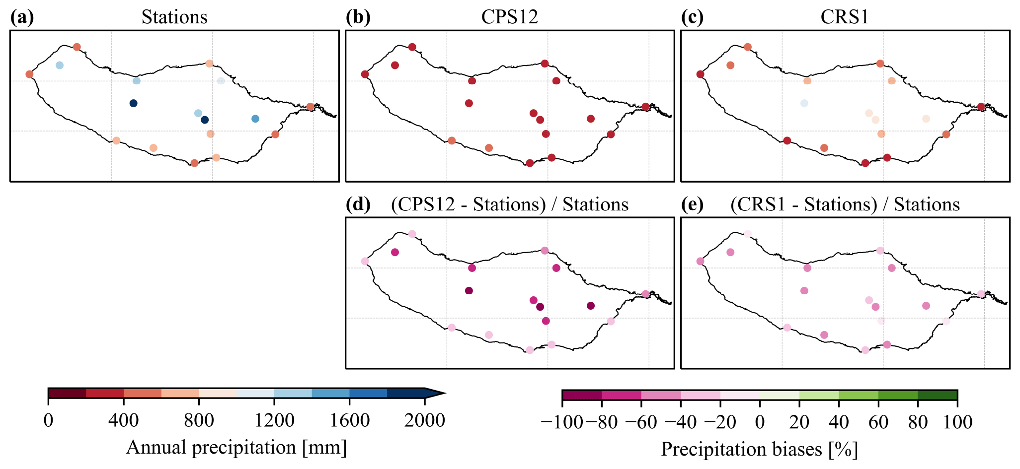
Figure C1Annual precipitation [mm] over (a–c) the analysis region and (d–f) the Madeira Archipelago in (a, d) the ERA5 reanalysis, (b, e) CPS12 and (c, f) CRS1 from 2006 to 2015. Note the different scales for the top and bottom row panels. The geographic map is from Natural Earth.
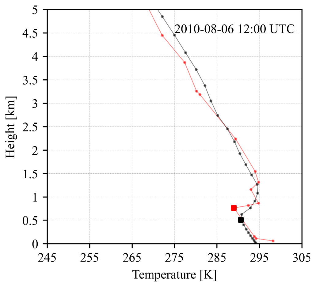
Figure C2Typical vertical temperature profiles at Funchal from the radiosonde observations (red line) and the model simulation (black line) on 6 August 2010 at 12:00 UTC. Nearest-neighbour interpolation is used to extract data from the model simulation at Funchal. The red and black squares represent the inversion height calculated from the vertical temperature profiles.
The ERA5 reanalysis can be obtained from the Climate Data Store (https://cds.climate.copernicus.eu; CDS, 2023). The ASCAT and MSG data are provided by EUMETSAT (https://navigator.eumetsat.int; EUMETSAT, 2023a), and the ASCAT Wind Data Processor (AWDP) is available from the OSI SAF (https://nwp-saf.eumetsat.int; EUMETSAT, 2023b). The radiosonde observations are from IGRA 2 (https://www.ncei.noaa.gov; NOAA, 2023). The observational station data are provided by the Portuguese Institute of Sea and Atmosphere and the Portuguese Environment Agency and are available upon request. The MODIS satellite data are from the NASA website (https://ladsweb.modaps.eosdis.nasa.gov; NASA, 2023). The digital elevation model of the Madeira Archipelago can be obtained from the European Environment Agency (https://sdi.eea.europa.eu, EEA, 2023). The maps in the figures are from Natural Earth (https://www.naturalearthdata.com/; Natural Earth, 2023) and GADM (https://gadm.org/; GADM, 2023). The model simulations are available from the authors upon request. The code for analysis can be found in the following GitHub repository: https://github.com/l975421700/DEoAI_analysis (Gao, 2023). The source code for generic cell identification that has been used for the first step of the rule-based vortex identification is available at https://doi.org/10.5281/zenodo.7506042 (Zeman and Canton, 2023).
Supplementary videos (four in total) can be found at Supporting Information: Vortex streets to the lee of Madeira in a km-resolution regional climate model (https://doi.org/10.5281/zenodo.7032529, Gao et al., 2021).
CS and JVT initiated and led the study. JVT conducted the decadal model simulation. QG and CZ contributed ideas in the early stage of the study. QG and CZ developed the code for the automatic vortex identification. QG performed the data analysis and created all figures and tables with contributions from CZ and DCAL. QG wrote the manuscript with contributions from all authors.
The contact author has declared that none of the authors has any competing interests.
Publisher's note: Copernicus Publications remains neutral with regard to jurisdictional claims in published maps and institutional affiliations.
We acknowledge PRACE (Partnership for Advanced Computing in Europe) for awarding us access to Piz Daint at the Swiss National Supercomputing Centre (CSCS). We also acknowledge the Federal Office for Meteorology and Climatology MeteoSwiss, CSCS and ETH Zurich for their contributions to the development of the GPU-accelerated version of COSMO. We would like to thank Jacopo Canton for his contribution to the development and testing of the generic cell identification algorithm. Daniela C. A. Lima would like to acknowledge the financial support by Pre-defined Project-2 National Roadmap for Adaptation XXI (PDP-2) funded by European Environment Agency (EEA) financial mechanism 2014–2021 and the Portuguese Environment Agency.
This work was supported by the European Union's Horizon 2020 research and innovation programme (EUCP, grant agreement no. 776613).
This paper was edited by Johannes Dahl and reviewed by two anonymous referees.
Abramovich, F., Bailey, T. C., and Sapatinas, T.: Wavelet Analysis and its Statistical Applications, J. Roy. Stat. Soc. D-Sta, 49, 1–29, https://doi.org/10.1111/1467-9884.00216, 2000. a
Azevedo, C. C., Camargo, C. M. L., Alves, J., and Caldeira, R. M. A.: Convection and Heat Transfer in Island (Warm) Wakes, J. Phys. Oceanogr., 51, 1187–1203, https://doi.org/10.1175/jpo-d-20-0103.1, 2020. a, b
Baldauf, M., Seifert, A., Förstner, J., Majewski, D., Raschendorfer, M., and Reinhardt, T.: Operational Convective-Scale Numerical Weather Prediction with the COSMO Model: Description and Sensitivities, Mon. Weather Rev., 139, 3887–3905, https://doi.org/10.1175/MWR-D-10-05013.1, 2011. a
Ban, N., Schmidli, J., and Schär, C.: Evaluation of the convection-resolving regional climate modeling approach in decade-long simulations, J. Geophys. Res.-Atmos., 119, 7889–7907, https://doi.org/10.1002/2014JD021478, 2014. a
Ban, N., Schmidli, J., and Schär, C.: Heavy precipitation in a changing climate: Does short-term summer precipitation increase faster?, Geophys. Res. Lett., 42, 1165–1172, https://doi.org/10.1002/2014GL062588, 2015. a
Ban, N., Rajczak, J., Schmidli, J., and Schär, C.: Analysis of Alpine precipitation extremes using generalized extreme value theory in convection-resolving climate simulations, Clim. Dynam., 55, 61–75, https://doi.org/10.1007/s00382-018-4339-4, 2020. a
Bretherton, C. S.: Insights into low-latitude cloud feedbacks from high-resolution models, Philos. T. Roy. Soc. A, 373, 1–19, https://doi.org/10.1098/RSTA.2014.0415, 2015. a
Caldeira, R. M. and Tomé, R.: Wake Response to an Ocean-Feedback Mechanism: Madeira Island Case Study, Bound.-Lay. Meteorol., 148, 419–436, https://doi.org/10.1007/s10546-013-9817-y, 2013. a
Carrillo, J., Guerra, J. C., Cuevas, E., and Barrancos, J.: Characterization of the Marine Boundary Layer and the Trade-Wind Inversion over the Sub-tropical North Atlantic, Bound.-Lay. Meteorol., 158, 311–330, https://doi.org/10.1007/s10546-015-0081-1, 2016. a, b
CDS: Welcome to the Climate Data Store, https://cds.climate.copernicus.eu, last access: 31 January 2023. a
Cormen, T. H., Leiserson, C. E., Rivest, R. L., and Stein, C.: Data structures for disjoint sets, in: Introduction to Algorithms, 2nd Edn., chap. 21, MIT Press, 498–524, ISBN 9780262531962, 2001. a
Couvelard, X., Caldeira, R. M., Araújo, I. B., and Tomé, R.: Wind mediated vorticity-generation and eddy-confinement, leeward of the Madeira Island: 2008 numerical case study, Dynam. Atmos. Oceans, 58, 128–149, https://doi.org/10.1016/j.dynatmoce.2012.09.005, 2012. a
Cropper, T.: The weather and climate of Macaronesia: past, present and future, Weather, 68, 300–307, https://doi.org/10.1002/wea.2155, 2013. a, b
Cropper, T. E. and Hanna, E.: An analysis of the climate of Macaronesia, 1865–2012, Int. J. Climatol., 34, 604–622, https://doi.org/10.1002/joc.3710, 2014. a
Davis, R. E., Hayden, B. P., Gay, D. A., Phillips, W. L., and Jones, G. V.: The North Atlantic Subtropical Anticyclone, J. Climate, 10, 728–744, https://doi.org/10.1175/1520-0442(1997)010<0728:TNASA>2.0.CO;2, 1997. a, b
Dee, D. P., Uppala, S. M., Simmons, A. J., Berrisford, P., Poli, P., Kobayashi, S., Andrae, U., Balmaseda, M. A., Balsamo, G., Bauer, P., Bechtold, P., Beljaars, A. C. M., van de Berg, L., Bidlot, J., Bormann, N., Delsol, C., Dragani, R., Fuentes, M., Geer, A. J., Haimberger, L., Healy, S. B., Hersbach, H., Hólm, E. V., Isaksen, L., Kållberg, P., Köhler, M., Matricardi, M., McNally, A. P., Monge-Sanz, B. M., Morcrette, J.-J., Park, B.-K., Peubey, C., de Rosnay, P., Tavolato, C., Thépaut, J.-N., and Vitart, F.: The ERA-Interim reanalysis: configuration and performance of the data assimilation system, Q. J. Roy. Meteor. Soc., 137, 553–597, https://doi.org/10.1002/qj.828, 2011. a, b
Doglioli, A. M., Blanke, B., Speich, S., and Lapeyre, G.: Tracking coherent structures in a regional ocean model with wavelet analysis: Application to Cape Basin eddies, J. Geophys. Res.-Oceans, 112, C05043, https://doi.org/10.1029/2006JC003952, 2007. a
Domingues, M. O., Mendes, O., and Da Costa, A. M.: On wavelet techniques in atmospheric sciences, Adv. Space Res., 35, 831–842, https://doi.org/10.1016/j.asr.2005.02.097, 2005. a
Durran, D. R.: Mountain Waves and Downslope Winds, in: Atmospheric Processes over Complex Terrain, American Meteorological Society, 59–81, https://doi.org/10.1007/978-1-935704-25-6_4, 1990. a
Durre, I. and Yin, X.: Enhanced radiosonde data for studies of vertical structure, B. Am. Meteorol. Soc., 89, 1257–1262, 2008. a
Durre, I., Vose, R. S., and Wuertz, D. B.: Overview of the integrated global radiosonde archive, J. Climate, 19, 53–68, https://doi.org/10.1175/JCLI3594.1, 2006. a
EEA: SDI – geospatial data catalogue, https://sdi.eea.europa.eu, last access: 31 January 2023. a
Epifanio, C. C.: Mountain Meteorology: Lee Vortices, in: Encyclopedia of Atmospheric Sciences, 2nd edn., Elsevier Inc., 84–94, https://doi.org/10.1016/B978-0-12-382225-3.00241-3, 2015. a, b
Etling, D.: On atmospheric vortex streets in the wake of large islands, Meteorol. Atmos. Phys., 41, 157–164, https://doi.org/10.1007/BF01043134, 1989. a, b, c, d
Etling, D.: An unusual atmospheric vortex street, Environ. Fluid Mech., 19, 1379–1391, https://doi.org/10.1007/s10652-018-09654-w, 2019. a, b
EUMETSAT: Data Services, https://navigator.eumetsat.int (last access: 31 January 2023), 2023a. a
EUMETSAT: Supporting the use of satellite data for NWP, https://nwp-saf.eumetsat.int (last access: 31 January 2023), 2023b. a
Figa-Saldaña, J., Wilson, J. J., Attema, E., Gelsthorpe, R., Drinkwater, M. R., and Stoffelen, A.: The advanced scatterometer (ASCAT) on the meteorological operational (MetOp) platform: A follow on for european wind scatterometers, Can. J. Remote Sens., 28, 404–412, https://doi.org/10.5589/m02-035, 2002. a
Fragoso, M., Trigo, R. M., Pinto, J. G., Lopes, S., Lopes, A., Ulbrich, S., and Magro, C.: The 20 February 2010 Madeira flash-floods: synoptic analysis and extreme rainfall assessment, Nat. Hazards Earth Syst. Sci., 12, 715–730, https://doi.org/10.5194/nhess-12-715-2012, 2012. a
Fuhrer, O., Osuna, C., Lapillonne, X., Gysi, T., Cumming, B., Bianco, M., Arteaga, A., and Schulthess, T. C.: Towards a performance portable, architecture agnostic implementation strategy for weather and climate models, Supercomput. Front. Innov., 1, 45–62, https://doi.org/10.14529/jsfi140103, 2014. a
Fuhrer, O., Chadha, T., Hoefler, T., Kwasniewski, G., Lapillonne, X., Leutwyler, D., Lüthi, D., Osuna, C., Schär, C., Schulthess, T. C., and Vogt, H.: Near-global climate simulation at 1 km resolution: establishing a performance baseline on 4888 GPUs with COSMO 5.0, Geosci. Model Dev., 11, 1665–1681, https://doi.org/10.5194/gmd-11-1665-2018, 2018. a
GADM: Maps and data, https://gadm.org/, last access: 31 January 2023. a
Gao, Q.: Analysis code for the manuscript “Vortex streets to the lee of Madeira in a kilometre-resolution regional climate model”, GitHub [code], https://github.com/l975421700/DEoAI_analysis, last access: 31 January 2023. a
Gao, Q., Zeman, C., Vergara-Temprado, J., Molnar, P., and Schär, C.: Supporting Information: Vortex streets to the lee of Madeira in a km-resolution regional climate model, Zenodo [video supplement], https://doi.org/10.5281/zenodo.7032529, 2021. a, b, c, d, e, f, g
Grubišić, V., Sachsperger, J., and Caldeira, R. M. A.: Atmospheric Wake of Madeira: First Aerial Observations and Numerical Simulations, J. Atmos. Sci., 72, 4755–4776, https://doi.org/10.1175/JAS-D-14-0251.1, 2015. a, b, c, d
Heinze, R., Raasch, S., and Etling, D.: The structure of Kármán vortex streets in the atmospheric boundary layer derived from large eddy simulation, Meteorol. Z., 21, 221–237, https://doi.org/10.1127/0941-2948/2012/0313, 2012. a, b, c, d, e, f, g, h
Hersbach, H., Bell, B., Berrisford, P., Hirahara, S., Horányi, A., Muñoz-Sabater, J., Nicolas, J., Peubey, C., Radu, R., Schepers, D., Simmons, A., Soci, C., Abdalla, S., Abellan, X., Balsamo, G., Bechtold, P., Biavati, G., Bidlot, J., Bonavita, M., De Chiara, G., Dahlgren, P., Dee, D., Diamantakis, M., Dragani, R., Flemming, J., Forbes, R., Fuentes, M., Geer, A., Haimberger, L., Healy, S., Hogan, R. J., Hólm, E., Janisková, M., Keeley, S., Laloyaux, P., Lopez, P., Lupu, C., Radnoti, G., de Rosnay, P., Rozum, I., Vamborg, F., Villaume, S., and Thépaut, J.-N.: The ERA5 global reanalysis, Q. J. Roy. Meteor. Soc., 146, 1999–2049, https://doi.org/10.1002/qj.3803, 2020. a
Horváth, Á., Bresky, W., Daniels, J., Vogelzang, J., Stoffelen, A., Carr, J. L., Wu, D. L., Seethala, C., Günther, T., and Buehler, S. A.: Evolution of an Atmospheric Kármán Vortex Street From High-Resolution Satellite Winds: Guadalupe Island Case Study, J. Geophys. Res.-Atmos., 125, e2019JD032121, https://doi.org/10.1029/2019JD032121, 2020. a, b
Hunt, J. C. and Snyder, W. H.: Experiments on stably and neutrally stratified flow over a model three-dimensional hill, J. Fluid Mech., 96, 671–704, https://doi.org/10.1017/S0022112080002303, 1980. a
Ito, J. and Niino, H.: Atmospheric Kármán Vortex Shedding from Jeju Island, East China Sea: A Numerical Study, Mon. Weather Rev., 144, 139–148, https://doi.org/10.1175/MWR-D-14-00406.1, 2015. a
Jawerth, B. and Sweldens, W.: An overview of wavelet based multiresolution analyses, SIAM Rev., 36, 377–412, https://doi.org/10.1137/1036095, 1994. a
Kahl, J. D.: Characteristics of the low-level temperature inversion along the Alaskan Arctic coast, Int. J. Climatol., 10, 537–548, https://doi.org/10.1002/joc.3370100509, 1990. a
Kármán, T. V.: On the mechanism of the drag a moving body experiences in a fluid, Prog. Aerosp. Sci., 59, 13–15, https://doi.org/10.1016/j.paerosci.2013.03.004, 2013. a, b
Klemp, J. B., Dudhia, J., and Hassiotis, A. D.: An Upper Gravity-Wave Absorbing Layer for NWP Applications, Mon. Weather Rev., 136, 3987–4004, https://doi.org/10.1175/2008MWR2596.1, 2008. a
Luna, T., Rocha, A., Carvalho, A. C., Ferreira, J. A., and Sousa, J.: Modelling the extreme precipitation event over Madeira Island on 20 February 2010, Nat. Hazards Earth Syst. Sci., 11, 2437–2452, https://doi.org/10.5194/nhess-11-2437-2011, 2011. a
McWilliams, J. C.: The vortices of two-dimensional turbulence, J. Fluid Mech., 219, 361–385, https://doi.org/10.1017/S0022112090002981, 1990. a, b
Mosimann, L.: Towards online cloud tracking with the COSMO-Model, Master thesis, ETH Zürich, 2016. a, b
NASA: LAADS DAAC, https://ladsweb.modaps.eosdis.nasa.gov, last access: 30 January 2023. a
Natural Earth: Coastline, https://www.naturalearthdata.com/, last access: 30 January 2023. a
Nencioli, F., Dong, C., Dickey, T., Washburn, L., and McWilliams, J. C.: A vector geometry-based eddy detection algorithm and its application to a high-resolution numerical model product and high-frequency radar surface velocities in the Southern California Bight, J. Atmos. Ocean. Tech., 27, 564–579, https://doi.org/10.1175/2009JTECHO725.1, 2010. a, b
NOAA: National Centers for Environmental Information, https://www.ncei.noaa.gov, last access: 31 January 2023. a
Nunalee, C. G. and Basu, S.: On the periodicity of atmospheric von Kármán vortex streets, Environ. Fluid Mech., 14, 1335–1355, https://doi.org/10.1007/s10652-014-9340-9, 2014. a, b
Nunalee, C. G., He, P., Basu, S., Minet, J., and Vorontsov, M. A.: Mapping optical ray trajectories through island wake vortices, Meteorol. Atmos. Phys., 127, 355–368, https://doi.org/10.1007/s00703-015-0366-4, 2015. a
Ramos, A. M., Trigo, R. M., Tomé, R., and Liberato, M. L. R.: Impacts of Atmospheric Rivers in Extreme Precipitation on the European Macaronesian Islands, Atmosphere, 9, 325, https://doi.org/10.3390/atmos9080325, 2018. a
Reynolds, D.: Gaussian Mixture Models, in: Encyclopedia of Biometrics, Springer US, Boston, MA, 827–832, https://doi.org/10.1007/978-1-4899-7488-4_196, 2015. a
Rockel, B., Will, A., and Hense, A.: The Regional Climate Model COSMO-CLM (CCLM), Meteorol. Z., 17, 347–348, https://doi.org/10.1127/0941-2948/2008/0309, 2008. a
Romps, D. M.: Exact expression for the lifting condensation level, J. Atmos. Sci., 74, 3891–3900, https://doi.org/10.1175/JAS-D-17-0102.1, 2017. a
Rotunno, R., Grubišić, V., and Smolarkiewicz, P. K.: Vorticity and Potential Vorticity in Mountain Wakes, J. Atmos. Sci., 56, 2796–2810, https://doi.org/10.1175/1520-0469(1999)056<2796:VAPVIM>2.0.CO;2, 1999. a
Ruppert-Felsot, J. E., Praud, O., Sharon, E., and Swinney, H. L.: Extraction of coherent structures in a rotating turbulent flow experiment, Phys. Rev. E, 72, 16311, https://doi.org/10.1103/PhysRevE.72.016311, 2005. a, b
Savtchenko, A., Ouzounov, D., Ahmad, S., Acker, J., Leptoukh, G., Koziana, J., and Nickless, D.: Terra and Aqua MODIS products available from NASA GES DAAC, Adv. Space Res., 34, 710–714, https://doi.org/10.1016/j.asr.2004.03.012, 2004. a
Schär, C.: A Generalization of Bernoulli's Theorem, J. Atmos. Sci., 50, 1437–1443, https://doi.org/10.1175/1520-0469(1993)050<1437:AGOBT>2.0.CO;2, 1993. a
Schär, C. and Durran, D. R.: Vortex Formation and Vortex Shedding in Continuously Stratified Flows past Isolated Topography, J. Atmos. Sci., 54, 534–554, https://doi.org/10.1175/1520-0469(1997)054<0534:VFAVSI>2.0.CO;2, 1997. a, b, c, d
Schär, C. and Smith, R. B.: Shallow-Water Flow past Isolated Topography. Part I: Vorticity Production and Wake Formation, J. Atmos. Sci., 50, 1373–1400, https://doi.org/10.1175/1520-0469(1993)050<1373:SWFPIT>2.0.CO;2, 1993a. a
Schär, C. and Smith, R. B.: Shallow-Water Flow past Isolated Topography. Part II: Transition to Vortex Shedding, J. Atmos. Sci., 50, 1401–1412, https://doi.org/10.1175/1520-0469(1993)050<1401:SWFPIT>2.0.CO;2, 1993b. a
Schär, C., Sprenger, M., Lüthi, D., Jiang, Q., Smith, R. B., and Benoit, R.: Structure and dynamics of an Alpine potential-vorticity banner, Q. J. Roy. Meteor. Soc., 129, 825–855, https://doi.org/10.1256/qj.02.47, 2003. a
Schielicke, L., Névir, P., and Ulbrich, U.: Kinematic vorticity number – a tool for estimating vortex sizes and circulations, Tellus A, 68, 29464, https://doi.org/10.3402/TELLUSA.V68.29464, 2016. a
Schmetz, J., Pili, P., Tjemkes, S., Just, D., Kerkmann, J., Rota, S., and Ratier, A.: An introduction to Meteosat Second Generation (MSG), B. Am. Meteorol. Soc., 83, 977–992, https://doi.org/10.1175/1520-0477(2002)083<0977:AITMSG>2.3.CO;2, 2002. a, b
Schneider, T., Kaul, C. M., and Pressel, K. G.: Possible climate transitions from breakup of stratocumulus decks under greenhouse warming, Nat. Geosci., 12, 163–167, https://doi.org/10.1038/s41561-019-0310-1, 2019. a
Sheppard, P. A.: Airflow over mountains, Q. J. Roy. Meteor. Soc., 82, 528–529, https://doi.org/10.1002/qj.49708235418, 1956. a, b
Siegel, A. and Weiss, J. B.: A wavelet-packet census algorithm for calculating vortex statistics, Phys. Fluids, 9, 1988–1999, https://doi.org/10.1063/1.869318, 1997. a
Smith, R. B. and Gronas, S.: Stagnation points and bifurcation in 3-D mountain airflow, Tellus A, 45, 28–43, https://doi.org/10.3402/TELLUSA.V45I1.14840, 1993. a
Smith, R. B. and Grubišić, V.: Aerial Observations of Hawaii's Wake, J. Atmos. Sci., 50, 3728–3750, https://doi.org/10.1175/1520-0469(1993)050<3728:AOOHW>2.0.CO;2, 1993. a, b
Smolarkiewicz, P. K. and Rotunno, R.: Low Froude number flow past three-dimensional obstacles. Part I: baroclinically generated lee vortices, J. Atmos. Sci., 46, 1154–1164, https://doi.org/10.1175/1520-0469(1989)046<1154:LFNFPT>2.0.CO;2, 1989. a
Snyder, W. H., Thompson, R. S., Eskridge, R. E., Lawson, R. E., Castro, I. P., Lee, J. T., Hunt, J. C. R., and Ogawa, Y.: The structure of strongly stratified flow over hills: dividing-streamline concept, J. Fluid Mech., 152, 249–288, https://doi.org/10.1017/S0022112085000684, 1985. a
Tsuchiya, K.: The Clouds with the Shape of Karman Vortex Street in the Wake of Cheju Island, Korea, J. Meteorol. Soc. Jpn. Ser. II, 47, 457–465, https://doi.org/10.2151/jmsj1965.47.6_457, 1969. a, b
Visbeck, M. H., Hurrell, J. W., Polvani, L., and Cullen, H. M.: The North Atlantic oscillation: Past, present, and future, P. Natl. Acad. Sci. USA, 98, 12876–12877, https://doi.org/10.1073/pnas.231391598, 2001. a
Vogelzang, J., Stoffelen, A., Lindsley, R. D., Verhoef, A., and Verspeek, J.: The ASCAT 6.25-km Wind Product, IEEE J. Sel. Top. Appl., 10, 2321–2331, https://doi.org/10.1109/JSTARS.2016.2623862, 2017. a
Wang, S.-H., Zhang, Y.-D., Dong, Z., and Phillips, P.: Wavelet Families and Variants, in: Brain Informatics and Health, Springer, Singapore, 85–104, https://doi.org/10.1007/978-981-10-4026-9_6, 2018. a
Wicker, L. J. and Skamarock, W. C.: Time-splitting methods for elastic models using forward time schemes, Mon. Weather Rev., 130, 2088–2097, https://doi.org/10.1175/1520-0493(2002)130<2088:TSMFEM>2.0.CO;2, 2002. a
Wickerhauser, M. V.: Adapted Wavelet Analysis From Theory to Software, A K Peters/CRC Press, New York, https://doi.org/10.1201/9781439863619, 1996. a
Yang, C., Zhao, H., Bruzzone, L., Benediktsson, J. A., Liang, Y., Liu, B., Zeng, X., Guan, R., Li, C., and Ouyang, Z.: Lunar impact crater identification and age estimation with Chang'E data by deep and transfer learning, Nat. Commun., 11, 6358, https://doi.org/10.1038/s41467-020-20215-y, 2020. a
Young, G. S. and Zawislak, J.: An Observational Study of Vortex Spacing in Island Wake Vortex Streets, Mon. Weather Rev., 134, 2285–2294, https://doi.org/10.1175/MWR3186.1, 2006. a, b, c
Zeman, C. and Canton, J.: zemanc/identify_cells: v1.0.0 (v1.0.0), Zenodo [code], https://doi.org/10.5281/zenodo.7506042, 2023. a
- Abstract
- Introduction
- Data and methods
- Results
- Conclusions
- Appendix A: The wavelet analysis for denoising
- Appendix B: Identified vortex statistics
- Appendix C: Extra figures
- Code and data availability
- Video supplement
- Author contributions
- Competing interests
- Disclaimer
- Acknowledgements
- Financial support
- Review statement
- References