Convection-parameterized and convection-permitting modelling of heavy precipitation in decadal simulations of the greater Alpine region with COSMO-CLM

Heavy precipitation is a challenging phenomenon with high impact on human lives and infrastructure, and thus a better modelling of its characteristics can improve understanding and simulation at climate timescales. The achievement of convection-permitting modelling (CPM) resolutions (Δx<4 km) has brought relevant advancements in its representation. However, further research is needed on how the very high resolution and switching-off of the convection parameterization affects the representation of processes related to heavy precipitation. In this study, we evaluate reanalysis-driven simulations for the greater Alpine area over the period 2000–2015 and assess the differences in representing heavy precipitation and other model variables in a CPM setup with a grid size of 3 km and a regional climate model (RCM) setup at 25 km resolution using the COSMO-CLM model. We validate our simulations against high-resolution observations (E-OBS (ENSEMBLES observations), HYRAS (Hydrometeorologische Rasterdatensätze), MSWEP (Multi-Source Weighted-Ensemble Precipitation), and UWYO (University of Wyoming)). The study presents a revisited version of the precipitation severity index (PSI) for severe event detection, which is a useful method to detect severe events and is flexible for prioritizing long-lasting events and episodes affecting typically drier areas. Furthermore, we use principal component analysis (PCA) to obtain the main modes of heavy precipitation variance and the associated synoptic weather types (WTs). The PCA showed that four WTs suffice to explain the synoptic situations associated with heavy precipitation in winter, due to stationary fronts and zonal flow regimes. Whereas in summer, five WTs are needed to classify the majority of heavy precipitation events. They are associated with upper-level elongated troughs over western Europe, sometimes evolving into cutoff lows, or with winter-like situations of strong zonal circulation. The results indicate that CPM represents higher precipitation intensities, better rank correlation, better hit rates for extremes detection, and an improved representation of heavy precipitation amount and structure for selected events compared to RCM. However, CPM overestimates grid point precipitation rates, which agrees with findings in past literature. CPM systematically represents more precipitation at the mountain tops. However, the RCMs may show large intensities in other regions. Integrated water vapour and equivalent potential temperature at 850 hPa are systematically larger in RCM compared to CPM in heavy precipitation situations (up to 2 mm and 3 K, respectively) due to wetter mid-level conditions and an intensified latent heat flux over the sea. At the ground level, CPM emits more latent heat than RCM over land (15 W m⁻²), bringing larger specific humidity north of the Alps (1 g kg⁻¹) and higher CAPE (convective available potential energy) values (100 J kg⁻¹). RCM, on the contrary simulates a wetter surface level over Italy and the Mediterranean Sea. Surface temperatures in RCM are up to 2 ^∘C higher in RCM than in CPM. This causes outgoing longwave radiation to be larger in RCM compared to CPM over those areas (10 W m⁻²). Our analysis emphasizes the improvements of CPM for heavy precipitation modelling and highlights the differences against RCM that should be considered when using COSMO-CLM climate simulations.

1 Introduction

Heavy precipitation events cause tremendous damages and casualties in central Europe (Alfieri et al., 2016; Khodayar et al., 2021; Ranasinghe et al., 2021). In a warming climate, the occurrence and intensity of such events is projected to increase as assessed in Sect. 8 of the Intergovernmental Panel on Climate Change (IPCC) and previous publications (Douville et al., 2021; Pichelli et al., 2021) due to the intensification of the hydrological cycle (Rajcack et al., 2013; Ban et al., 2018). Such events may occur during both winter and summer, fostered by deep moist convection (DMC), a large vertical transport of precipitating air masses (Emanuel, 1994). In winter, heavy precipitation typically occurs under strong synoptic forcing (Keil et al., 2020), caused by the large-scale advection of positive vorticity in cold upper-level layers (Holton, 2013). The associated synoptic patterns have been studied in past literature (e.g. Knippertz et al., 2003; Werner and Gerstengarbe, 2010; Stucki et al., 2012), referring a strong influence of northerly cutoff geopotential lows and elongated troughs as well as of the Atlantic zonal flow. In summer, DMC is often triggered by favourable local and mesoscale conditions close to the surface, including a warm and moist low-level and a triggering mechanism (Doswell et al., 1996). When these conditions coincide with the arrival of a mesoscale low-pressure system, highly damaging precipitation is likely to occur.

Understanding heavy precipitation processes, their variability, and trends at decadal timescales is needed to provide better prevention and adaptation strategies. Considering modelling approaches, dynamical downscaling with regional climate models (RCMs) has proven to be a valuable tool towards this end (e.g. Jacob et al., 2014). Recently, the development of convection-permitting models (CPMs) led to a step forward (Coppola et al., 2018; Prein et al., 2020; Lucas-Picher et al., 2021) since a parameterized description of deep convection is no longer needed. An explicit representation of convection is often applied for horizontal grid spacings lower than ca. 5 km. Also improved is the representation of the model's land type, use, and elevation (Prein et al., 2015; Heim et al., 2020). These advancements led to improvements in representing the daily precipitation's diurnal cycle (Kendon et al., 2012; Berthou et al., 2018; Ban et al., 2021); its structure, intensity, frequency, and duration (Berthou et al., 2019; Berg et al., 2019); its sub-hourly rates (Meredith et al., 2020); and its orographic triggering (Ban et al., 2018). These improvements are consistent over the main modelling regions worldwide. However, not all problems are solved, since CPMs have also shown relevant wet biases, inducing an overestimation of extreme intensities (Kendon et al., 2012). CPM uncertainties arise from shortcomings in the physical parameterizations, the coupling of the numerics and the physics-dynamics, deficiencies in the representation of the initial conditions, and the lack of sufficient high-resolution observations for validation (Lucas-Picher et al., 2021).

Particularly relevant for the improvement of heavy precipitation in CPM is the better representation of DMC processes, especially when convection is triggered close to the surface (Bui et al., 2018). In fact, studies have shown that CPMs induce stronger updraughts that lead to stronger convection (Meredith et al., 2015a, b). This is also observed in numerical weather prediction (NWP) simulations (Barthlott and Hoose, 2015; Panosetti et al., 2018). When convection occurs over an area of complex orography, the finer representation of the mountains in CPM increases the triggering of convection (Langhans et al., 2012; Vanden-Broucke et al., 2018; Heim, 2018; Vergara-Temprado et al., 2020), leading to a better agreement with radar observations (Purr et al., 2019). Regarding other model variables, previous papers argued that CPM improves the simulation of surface temperature (Ban et al., 2014; Prein et al., 2015; Hackenbruch et al., 2016), due to a better representation of the orography, as well as the cloud coverage (Lucas-Picher et al., 2021). Regarding the soil-moisture–precipitation feedback, past work has shown that RCM tends to show a positive sign (Hohenegger et al., 2009; Leutwyler et al., 2021), whereas CPM can show both negative and positive signs at the sub-continental and continental spatial scales, respectively. The reason is that wetter soils induce more frequent precipitation at RCMs but more intense events in CPM (Leutwyler et al., 2021). CPM seems to better agree with observations, as previous observations showed a negative sign of the feedback, due to an increased sensible heat flux over drier soils, and mesoscale variability in soil moisture, which intensifies afternoon convection (Taylor et al., 2012). Moisture biases also affect the development of heavy precipitation, where a wet bias was found for established RCM models (Lin et al., 2018; Li et al., 2020) as well as in CPM simulations (Risanto et al., 2019; Bastin et al., 2019; Caldas-Alvarez and Khodayar, 2020; Li et al., 2020). However, how both RCM and CPM deal with the moisture wet bias is still an open question. Regarding atmospheric instability, Li et al. (2020) found larger convective available potential energy (CAPE) during the afternoon in CPM, which was correctly converted to higher precipitation at the Tibetan Plateau. Finally, the scale dependency of other variables of interest for convective development, such as equivalent potential temperature at 850 hPa (${\mathit{\theta }}_{\mathrm{e}}^{\mathrm{850}}$), has seldom been investigated.

The model evaluated in this paper is the Consortium for Small-scale Modelling in Climate Mode (COSMO-CLM; Schättler et al., 2016; Rockel et al., 2008), which is especially suitable for studying differences between RCM and CPM due its flexibility for configuration in convection-parameterized and convection-permitting resolutions. COSMO-CLM is a well established regional climate model used by research and applied-science institutions in Europe (Sørland et al., 2021), and hence there is interest in quantifying its skill in simulating heavy precipitation and its associated processes in a CPM setup.

One established technique to work with large datasets, such as decadal climate simulations, is principal component analysis (PCA). PCA is a powerful method to reduce the dimensionality of a set (Joliffe, 2002) and to extract the principal underlying features. One of its applications is the derivation of the leading spatial patterns of atmospheric fields during specific situations, e.g. heavy precipitation (Knippertz et al., 2003; Seregina et al., 2021). Provided PCA also calculates the correlation between the days of the set and the derived spatial patterns, it can be used to construct composite maps of relevant model variables associated with the respective spatial patterns of a specific model variable, e.g. precipitation. Although PCA has been used for these applications in the past, to our knowledge, it has not yet been applied to study model differences between RCM and CPM. In this work we will derive composites of relevant model variables and study differences between both modelling setups.

The aim of this work is to evaluate reanalysis-driven RCM (25 km) and CPM (3 km) decadal-long simulations of the greater Alpine area in the period 2000–2015 and assess their differences in representing heavy precipitation and associated environments. This paper is organized as follows: in Sect. 2 we introduce the dataset and methods employed; in Sect. 3 we present the main synoptic weather types bringing heavy precipitation; in Sect. 4 we evaluate heavy precipitation intensity and occurrence in the decadal simulations; in Sect. 5 we validate precipitation, humidity, and temperature fields of selected heavy precipitation events; in Sect. 6 we introduce the spatial patterns of precipitation derived from PCA; in Sect. 7 we present the differences of model variable composites; and in Sect. 8 we provide our conclusions.

1.1 Observational datasets

We use observations from various sources for validation and comparison of the climate simulations (Table 1). We employ the ENSEMBLES observations (E-OBS) gridded precipitation and relative humidity at the surface (hurs) products at 25 km resolution (E-OBS-25 km), which are provided by the European Climate Assessment & Dataset (ECA&D) centre at 0.25^∘ (ca. 25 km) of spatial resolution for the period 1950–2020. We use v.22.0e (December 2020), employing a 100-member ensemble created through stochastic simulations based on interpolated station data from national institutions including 9000 rain gauges (Cornes et al., 2018). E-OBS-25 km has been widely used in previous literature for validation purposes (e.g. Tramblay et al., 2019; Bandhauer et al., 2021) and has been shown to have low median absolute biases with respect to other regional European precipitation products such as CARPATCLIM or Spain02 (Cornes et al., 2018).

Table 1 Description of observational datasets used for validation. The observational data types used to create the products are radar (R), gauges (G), satellites (S), and reanalysis (R).

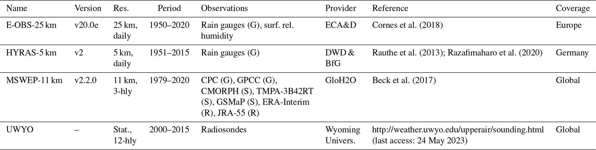
The Hydrometeorologische Rasterdatensätze (HYRAS) gridded precipitation dataset, provided by the German Weather Service (DWD), is available at 1 km (ca. 0.01^∘), 5 km (ca. 0.05^∘), and daily resolution. HYRAS covers Germany and neighbouring catchments in parts of Switzerland, Austria, the Netherlands, France, Belgium, and Poland (Fig. 1). The version v2 covers the period 1951–2015 and was derived using multiple linear regression and inverse distance weighting interpolation of 6200 rain gauges considering the orography (Rauthe et al., 2013; Razafimaharo et al., 2020). HYRAS-5 km has a remarkable quality, and its high resolution enables a good representation of local scale features, outperforming the coarse resolution of E-OBS-25 km (Hu and Franzke, 2020). However, it is only available over Germany and nearby catchments.

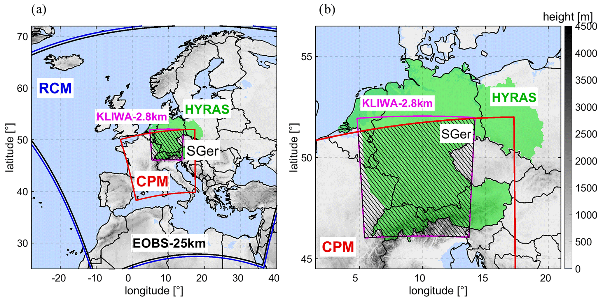
Figure 1 (a) Simulation and observation domains for RCM (25 km; blue), CPM (3 km; red), KLIWA-2.8 km (magenta), HYRAS-5 km (green), and E-OBS-25 km (black). The two investigation domains of this study are southern Germany (SGer; dashed box) and the CPM domain. (b) Zoom into the area of interest.

The Multi-Source Weighted-Ensemble Precipitation (MSWEP) is a gridded precipitation product provided by GloH2O (http://www.gloh2o.org/, last access: 24 May 2023) at 0.1^∘ (ca. 11 km) spatial resolution and 3-hourly temporal resolution for the period 1979–2020 with global coverage. We use version v.2.2.0., which was obtained through weighted interpolation of different observations to a common grid. It merges data from rain gauge observations from the Climate Prediction Center (CPC) unified and Global Precipitation Climatology Centre (GPCC), satellite observations from the CPC MORPHing product (CMORPH), Global Satellite Mapping Precipitation Moving Vector with Kalman (GSMaP-MVK), and Tropical Rainfall Measuring Mission Multi-satellite Precipitation Analysis (TMPA) 3B42, as well as two reanalysis datasets ERA-Interim and Japanese Reanalysis JRA-55 (Beck et al., 2019). MSWEP has a higher median correlation (up to 0.67) against stations compared to CMORPH (0.44) and TMPA-3B42 (0.59) (Beck et al., 2017). We use the MSWEP product to profit from its high accuracy, shown in previous studies, globally (Beck et al., 2017, 2019; Xiang et al., 2021) as well as in specific geographies (Du et al., 2022; Peña-Guerrero et al., 2022). MSWEP has the advantage of covering sea surfaces and is adequate for precipitation event evaluation because it includes gauge data from CPC and GPCC.

The radiosonde data archived by the University of Wyoming (UWYO) are used to validate the RCM and CPM humidity and temperature profiles. The stations are located close to large European cities, with an average distance of 250 km between stations. The temporal resolution ranges between 6, 12, and 24 h, and the provided information includes height, atmospheric pressure, temperature, and dew point temperature on ca. 30 levels. The UWYO soundings have often been used as reference for validation studies (e.g. Ciesileski et al., 2014; Yang et al., 2020).

1.2 Setup of the COSMO-CLM, RCM, and CPM simulations

We use COSMO-CLM, a non-hydrostatic model using the fully compressible atmospheric equations (Schättler et al., 2016), incorporating sub-grid turbulence, convection, and grid-scale clouds and precipitation parameterizations. COSMO-CLM uses a soil model called TERRA-ML (Doms et al., 2013) to parameterize the mass and heat exchanges between the surface and the atmosphere (Rockel et al., 2008).

In this work, we systematically compare reanalysis-driven regional climate simulations with a typical RCM resolution (25 km; hereafter named RCM) and at a convection-permitting resolution (∼3 km, named CPM). All simulations were performed with the version COSMO-CLM5 and use a setup specifically optimized for these resolutions.

The RCM simulation covers the period 1961–2018 (Table 2), has a grid spacing of 0.22^∘ (ca. 25 km), has a 3-hourly output, and was performed within the scope of the MiKlip project (Feldmann et al., 2019). This simulation was performed for the EURO-CORDEX domain (Jacob et al., 2014) and thus covers the European continent and vast areas of the North Atlantic and the Mediterranean (Fig. 1). The RCM simulation is forced by ERA-Interim (Dee et al., 2011) for the period investigated in this paper (2000–2015). The setup is that recommended for COSMO-CLM5 for typical RCM resolutions (10–50 km). The most relevant model settings are summarized in Table 2 and in Sørland et al. (2021).

Table 2 Reanalysis-driven COSMO-CLM decadal simulations.

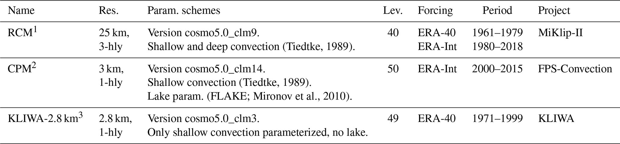
¹ Domain covers from the Atlantic to the eastern Mediterranean and from the Maghreb area to Iceland and Scandinavia. ² Domain covers France, northern Italy, Switzerland, the Czech Republic, southern Germany, and the Mediterranean. ³ Simulations provided by the KLIWA project (https://www.kliwa.de/, last access: 24 May 2023: Hundhausen et al., 2022). Domain covers southern Germany, Switzerland, and the eastern Czech Republic.

The CPM simulation uses a COSMO-CLM5 subversion with a few bug fixes and additional output variables but no changes in the numerics or formulation of the physics. The setup has been optimized for convection-permitting scales and is used in the CORDEX Flagship Pilot Study on Convection (Coppola et al., 2018), and the simulation has been evaluated in Ban et al. (2021). This means that there are differences in the specific tuning parameters, where the main difference is the switching of the deep-convection parameterization (Tiedtke, 1989; Baldauf et al., 2011; see Table 2). The simulation is performed by downscaling the RCM simulation described above over the grater Alpine area (ALP-3) domain, with a 3 km (0.0275^∘) resolution for the period 2000–2015.

Another convection-permitting simulation – here called KLIWA-2.8 km (see Table 2) – is used as an auxiliary just in Sect. 4 (Fig. 6) to extend the period for the comparison of the historical events. The grid spacing of this simulation is 2.8 km (0.025^∘) and covers a smaller modelling domain over southern Germany and the Alps (see Fig. 1) for the period 1971–2000. It is forced by ERA-40 re-analysis (Uppala et al., 2005) in a three-step nesting approach (Hundhausen et al., 2022). This simulation uses a slightly older subversion, missing a few bug fixes. The main differences to CPM can be found in Table 2.

Two areas are investigated in our study. The first, denominated southern Germany (SGer, Fig. 1), encompasses the northern Alps and southern Germany up to North Rhine-Westphalia and Saxony. This area is selected to fulfil the requirements of the modelling and observational datasets (availability, coverage, time span). The second area, CPM (Fig. 1), covers the greater Alpine domain including the northern Mediterranean basin and is used for comparison of the model performance RCM vs. CPM.

1.3 Analytical methods

1.3.1 The precipitation severity index (PSI)

We re-adapted the PSI, an index previously used to detect heavy precipitation events (Piper et al., 2016) and severe windstorms (Leckebusch et al., 2008; Pinto et al., 2012), to include precipitation persistence. By doing so we can consider three different but intertwined aspects of heavy precipitation: grid-point intensity, spatial extent of affected area, and temporal persistence. It is re-defined as follows:

$$\begin{array}{}\text{(1)}& \begin{array}{rl}{\mathrm{PSI}}_T& ={\displaystyle \frac{\mathrm{1}}{(\mathrm{1}+d)\cdot A}}\sum _{i=\mathrm{1}}^N\sum _{j=\mathrm{1}}^M\sum _{t=T-d}^T{\displaystyle \frac{{\mathrm{RR}}_{ijt}}{{\mathrm{RR}}_{{\mathrm{perc}}_{ij}}}}\cdot (\mathrm{\Delta }x{)}^{\mathrm{2}}\\ & \cdot \prod _{\mathit{\tau }=t}^{T}I\left({\mathrm{RR}}_{ij\mathit{\tau }},R{R}_{{\mathrm{perc}}_{ij}}\right)\end{array}\end{array}$$

$$I\left({\mathrm{RR}}_{ij\mathit{\tau }},{\mathrm{RR}}_{{\mathrm{perc}}_{ij}}\right)=\left\{\begin{array}{cc}\mathrm{0}& \mathrm{if}{\mathrm{RR}}_{ij\mathit{\tau }}\le {\mathrm{RR}}_{{\mathrm{80}}_{ij}}\\ \mathrm{1}& \mathrm{if}{\mathrm{RR}}_{ij\mathit{\tau }}>{\mathrm{RR}}_{{\mathrm{80}}_{ij}}\end{array}\right..$$

The PSI values at a certain time step T (PSI_T) are obtained from the ratio between grid point daily precipitation (RR_ijt) and a user-defined threshold. In this paper we set this threshold to be the all-day 80th percentile (${\mathrm{RR}}_{{\mathrm{perc}}_{ij}}$) to neglect grid points whose precipitation is lower than the set threshold for day T (${\mathrm{RR}}_{ij\mathit{\tau }}\le {\mathrm{RR}}_{{\mathrm{perc}}_{ij}}$). This is done by means of the function I(RR_ijτ, ${\mathrm{RR}}_{{\mathrm{perc}}_{ij}})$. We consider the spatial extent by summing the ratios over the spatial extent (N×M) of the study region along the directions i and j. The ratios are multiplied by the area of one grid cell (Δx)². The precipitation persistence is considered in the calculation through the sum over time (t). The ratios at each grid point for day T and the previous d days (d=2 in our case) are added for the PSI calculation, provided precipitation was continuous and larger than ${\mathrm{RR}}_{{\mathrm{perc}}_{ij}}$ at that same grid point i, j. The daily PSI value is normalized to the area of the simulation domain $A=N\cdot M\cdot (\mathrm{\Delta }x{)}^{\mathrm{2}}$ multiplied by (1+d) to consider the addition of grid points with persistent precipitation. Prior to the PSI calculation, we include a correction for latitude stretching of the grid as $\sqrt{\left(\cos \right(\mathrm{lat}\left)\right)}$, following (North et al., 1982).

To assess the performance of the PSI, we calculate Spearman's rank correlations between the PSI and a simpler field sum index (fldsum). We use daily precipitation data from HYRAS-5 km between 1 January 1971 and 31 December 2015 over the investigation area, SGer (Fig. 1). We evaluate different combinations of the PSI parameters ${\mathrm{RR}}_{{\mathrm{perc}}_{ij}}$ and d (Eq. 1). Figure 2 shows the rank correlations against fldsum and the three top-ranked events of each implementation and the daily precipitation of the 22 October 1986 event.

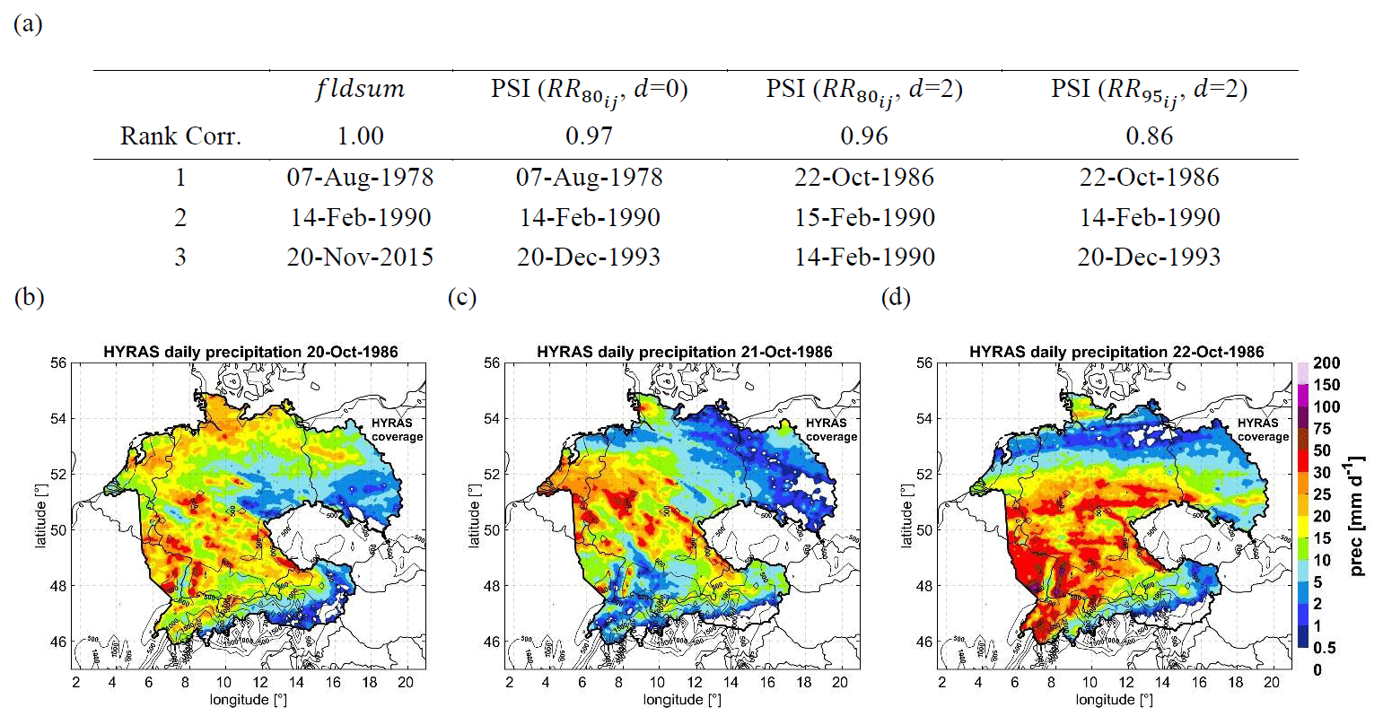
Figure 2 (a) Rank correlations between fldsum and different configurations of the PSI daily values in the period 1971–2015 over SGer, obtained with HYRAS-5 km. The top three events of the period are shown for each index. (b)–(d) Spatial distributions of daily precipitation measured by HYRAS-5 km on 20, 21, and 22 October 1986.

We find a high rank correlation between the PSI and fldsum for low values of ${\mathrm{RR}}_{{\mathrm{perc}}_{ij}}$ and d. For instance, when we set ${\mathrm{RR}}_{{\mathrm{perc}}_{ij}}$ as the 80th percentile of the 1971–2015 period and d=0 (equivalent to considering no persistent precipitation), the rank correlation is 0.97, indicative of a very similar functionality between the PSI and fldsum (Fig. 2a). In this configuration the third event in the ranking differs between the PSI (20 December 1993) and fldsum (20 November 2015). The reason behind is that the 20 December 1993 event occurred over a flat area, infrequently affected by heavy precipitation (Fig. S1 in the Supplement; SM). The PSI ranks 20 November 2015 as the third most extreme (affecting complex terrain) because the threshold set to the 80th percentile is lower over flat terrain and thus easier to surpass (Fig. S1).

As we increase ${\mathrm{RR}}_{{\mathrm{perc}}_{ij}}$ and d, the rank correlation decreases, implying a different ranking of the events (Fig. 2a). For example, a 95th percentile for ${\mathrm{RR}}_{{\mathrm{perc}}_{ij}}$ and d=2 brings a rank correlation of 0.86, which favours the detection of events with larger grid-point intensity and temporal persistence. For illustration, the 22 October 1986 event (Fig. 2b–d) is ranked as the most severe event in the period in this configuration due to precipitation totals between 50 and 150 mm d⁻¹ impacting the same areas for three consecutive days, e.g. the Colmar region or the Marburg–Siegen area (see Fig. 2b–d).

To conclude, the advantage of the PSI with respect to a simpler field sum index is its capability to detect rarer and more persistent events. Rarer events can be found because the threshold ${\mathrm{RR}}_{{\mathrm{perc}}_{ij}}$ guarantees the selection of events where either heavy precipitation falls over climatologically drier areas or extreme intensities take place over typically wet areas (e.g. complex terrain). For its part, d=2 favours the detection of events where heavy precipitation occurred continuously on the same grid point up to a maximum of 2 d. That said, a low percentile threshold (${\mathrm{RR}}_{{\mathrm{perc}}_{ij}}$) or d=0 will bring a functionality no different to fldsum. This makes the PSI a flexible solution that can be tailored to the user's needs. Finally, the PSI is also flexible for setting the threshold ${\mathrm{RR}}_{{\mathrm{perc}}_{ij}}$ to a fixed amount, e.g. 120 mm d⁻¹, to ensure that only grid points above that threshold will be included in the calculation. This is a configuration that could be used in future studies.

1.3.2 Principal component analysis

Principal component analysis (PCA) is a method to reduce the dimensionality of a dataset by transforming it to a new coordinate system of variables called principal components (PCs; Joliffe, 2002). The functions that allow the transformation from the original set to the PC space are called empirical orthogonal functions (EOFs). The transformation is performed in such a way that the explained variance is concentrated in a small number of components. By construction, the leading EOF-1 has the largest explained variance, followed by EOF-2, and so on. In this paper, we investigate the PCs and EOFs of 500 hPa geopotential height fields (Sect. 3) and daily precipitation (Sect. 6). Similarly to Ulbrich et al. (1999), we obtain EOFs representing the spatial patterns of the target variable that account for the main modes of variance. On the other hand, the PCs are time series which provide the information of the correlation of each EOF to a specific day in the series.

Given that the explained variance is now concentrated in a small number of variables, it is important to discern how many EOFs should be retained. With this aim, we use a method of parallel analysis based on the randomization of eigenvalues named the random-λ rule (Peres-Neto et al., 2005). The procedure is as follows: (1) a random data array is created with the same dimensions as the data array under study, (2) PCA is applied on the random array, and (3) steps 1 and 2 are repeated up to 1000 times, retaining the eigenvalues showing a significance over 95 % (α=0.05). (4) If the original eigenvalues exceed the critical values from the random data, then we reject the null hypothesis (Peres-Neto et al., 2005). The random-λ rule is more suitable than other methods of parallel analysis such as the N-rule (Preisendorfer, 1988), since it does not assume a normal distribution for the array of random values and thus works better for variables such as precipitation.

1.3.3 Validation metric fractions skill score

The fractions skill score (FSS) provides an estimation of the model's skill in representing the fraction of surface affected (or not) by heavy precipitation (Skok and Roberts, 2016). A perfect forecast thus has an FSS of 1. A simulation with no skill has an FSS of 0. In this work, we set a threshold of 40 mm d⁻¹ to define structures affected by heavy precipitation. The threshold is in the range of values implemented by Roberts and Lean (2008) for simulations of spring convective rain over southern England. We select this threshold to be able to identify clear precipitation structures otherwise masked by the choice of a too-large or too-low threshold analogously to Caldas-Alvarez et al. (2021). Equation (2) defines the FSS following Roberts and Lean (2008).

$$\begin{array}{}\text{(2)}& \mathrm{FSS}=\mathrm{1}-{\displaystyle \frac{\frac{\mathrm{1}}{M}\sum _{i=\mathrm{1}}^M{\left(f_{\mathrm{mod}}-f_{\mathrm{obs}}\right)}^{\mathrm{2}}}{\frac{\mathrm{1}}{M}\left(\sum _{i=\mathrm{1}}^M{f}_{\mathrm{mod}}^{\mathrm{2}}+\sum _{i=\mathrm{1}}^M{f}_{\mathrm{obs}}^{\mathrm{2}}\right)}}\end{array}$$

The fractions of surface affected by heavy precipitation are represented by f_obs and f_mod, for the observations and the model, respectively. Both are calculated as the number of grid points affected by precipitation over the defined threshold (40 mm d⁻¹) divided by the total number of grid points of a domain. FSS is computed as the ratio of the sums of fraction differences for M sub-boxes within the investigation domain. These M sub boxes are defined as sub-domains around M grid points with N near neighbours. N in our case is 12 since most of the events we validate have shown a skill larger than the target skill, defined as ${\mathrm{FSS}}_{\mathrm{target}}=\mathrm{0.5}+f_{\mathrm{obs}}/\mathrm{2}$ for N=12. For a detailed explanation, refer to Roberts and Lean (2008), Skok and Roberts (2016), and Caldas-Alvarez et al. (2021).

2 Synoptic weather types

We obtain the predominant large-scale situations associated with heavy precipitation by applying PCA. We analyse the EOFs of geopotential height at 500 hPa, based on the RCM simulation, for the period 1971–2015. We select dates of heavy precipitation in the 98-percentile of severity (PSI) in the HYRAS-5 km “all-day” dataset over the investigation region SGer (Fig. 1). Figures 3 and 4 provide, respectively, the dominating weather types of heavy precipitation for winter (SONDJF) and summer (MAMJJA). The comparison against the CPM is not shown here since only negligible differences exist with respect to RCM, since the boundary conditions from the forcing reanalyses (ERA) strongly determine the large-scale features (Prein et al., 2015).

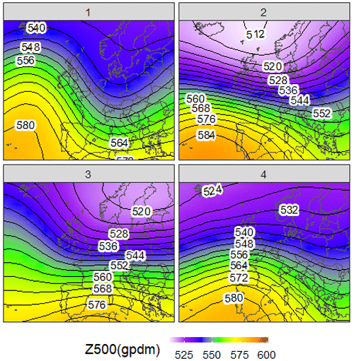
Figure 3 Synoptic weather patterns based on principal component analyses for the 98th percentile most severe precipitation cases in the region SGer in winter (SONDJF) of the 1971–2015 period, detected with the PSI. The spatial distributions show 500 hPa geopotential height in geopotential decametres (gpdm) obtained from RCM. The analysis has been performed with the synoptReg R package (Lemus-Canovas et al., 2019).

Table 3 Selected heavy precipitation events by means of the PSI between 2000–2015 including the PSI values, total precipitation, maximum grid point precipitation, and coverage (percentage of area affected by precipitation over the 80th percentile), obtained from HYRAS-5 km.

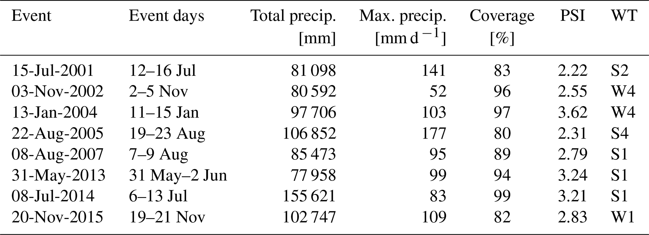
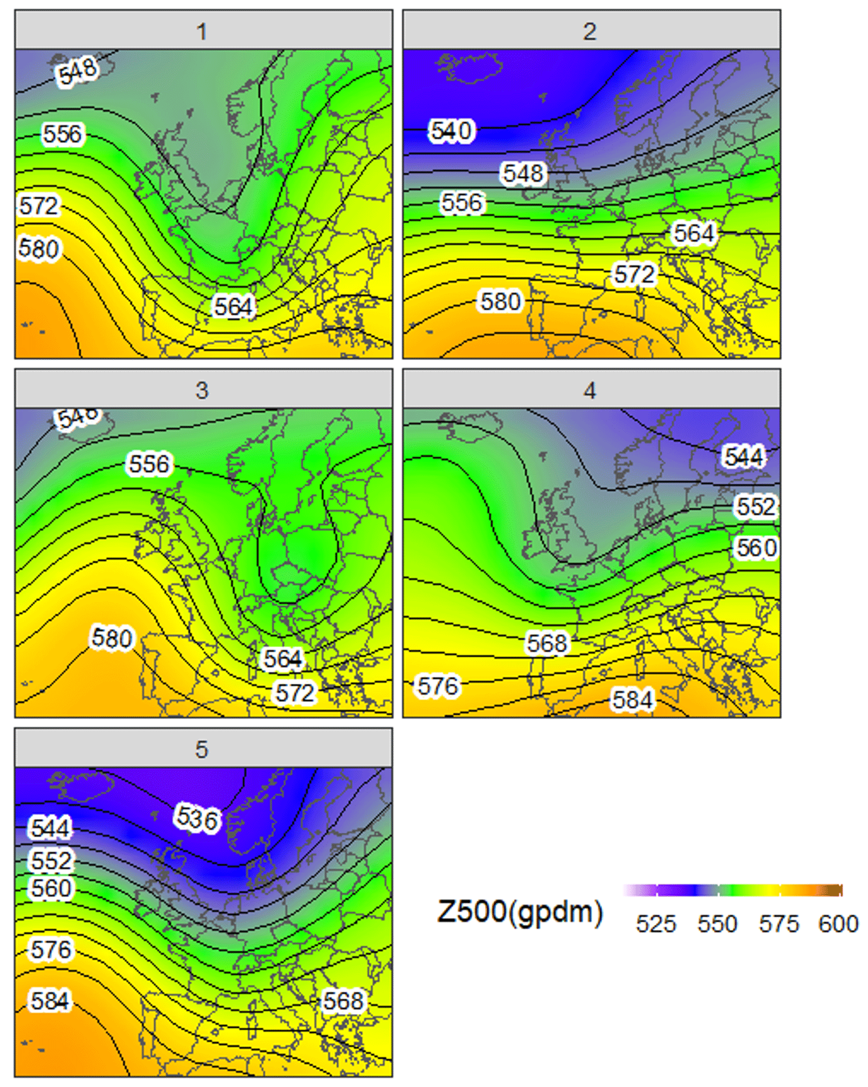
Figure 4 As Fig. 3 but for summer extreme precipitation days (MAMJJA).

In winter, four synoptic patterns of 500 hPa geopotential height suffice to explain the majority of HP events, following the random-λ rule with a 95 % significance in the t test (Peres-Neto et al., 2005). They account for 74 % of the heavy precipitation episodes. The first mode, representing 29 % of the events, is characterized by wave trains of low pressure associated with northerly incursions of polar air (Fig. 3). The synoptical situation is analogue to the stationary fronts (STFs) category proposed by Stucki et al. (2012). In this situation, heavy precipitation over the Alps is associated with strong upper-level lifting over northern Italy and large south-westerly advection of moisture from the Mediterranean. Historical cases belonging to this category, as identified by the PCA, are the second phase of the 23–31 October storms in 1998 (Fuchs et al., 1998) or the late November events in 2015 (Table 3, https://www.wetter.de/cms/so-war-das-wetter-im-november-2015-2566771.html, last access: 24 May 2023), for instance. The second mode, accounting for 22 % of the events, shows strong north–south gradients of the 500 hPa height and fast zonal circulations (Fig. 3). This synoptic pattern has been identified as a zonal flow (ZOW; Stucki et al., 2012) or as a narrow and elongated streamer (Massacand et al., 1998). The zonal circulation favours moisture advection from the Atlantic and can produce large precipitation in non-convective environments (Stucki et al., 2012). The 29 December 2001 event belongs to this precipitation mode, for instance. The third and fourth modes account for 12 % and 11 % of precipitation episodes, respectively, and show similarities with the 500 hPa geopotential heights of the second mode (Fig. 3). However, the third synoptic pattern shows a weaker Azores high, favouring the advection of Atlantic moisture with a south-westerly component. The fourth mode, for its part, shows a weaker polar low, which favours the development of anti-cyclonic circulation (Fig. 3).

In summer, five synoptic patterns of 500 hPa geopotential height are discernible from random noise (Peres-Neto et al., 2005), accounting for 77 % of the events. The first mode, corresponding to 27 % of the considered dates, shows an extended upper-level trough from the British Isles down to southern France (Fig. 4). This configuration shows elements of an elongated cutoff (ECO) and of Canarian troughs (CAT; Stucki et al., 2012). In such situations upper-level lifting occurs east of the trough together with southerly moisture advection either from the south-west or the south-east, respectively. Such situation occurred, for instance, during the first stages of the large central European flooding of early June 2013 (Kelemen et al., 2016). If a blocking situation occurs, for instance Omega blocking, the persistence of precipitation is enhanced and can lead to recurrent events (Kautz et al., 2022) at the eastern flank of the ECO or CAT. The second summer precipitation mode (Fig. 4), accounting for 19 % of the events, presents a similar pattern to the third and fourth modes of winter precipitation (Fig. 3), with the characteristic strong zonal flow from the Atlantic. Examples of this synoptic configuration are the March 1988 events flooding the Rhine river (south-western Germany; Prellberg and Fell, 1989) or the 15 June 2007 events affecting southern Germany (https://www.wetteronline.de/extremwetter/schwere-gewitter-und-starkregen-schaeden-durch-tief-, last access: 24 May 2023). The third precipitation mode, explaining 12 % of the analysed days (Fig. 4), shows similarly to the first mode, an ECO, however, with an eastward shifting of the Azores ridge and the possibility of evolving to a pivoting cutoff low (PCO; Stucki et al., 2012). If the PCO finally realizes and reaches the Mediterranean, it is accompanied by a cyclonic flow, which advects moisture towards central Europe and which originates in the Balkan region. This has been demonstrated to be the case for the second phase of the June 2013 flooding (Kelemen et al., 2016). The fourth summer precipitation mode (Fig. 4) accounts for 11 % of the considered episodes and represents situations of north-easterly development of the upper-level trough. The low pressure evolves into a CAT situation, inducing a south-westerly moist inflow to the Alpine region (Stucki et al., 2012). The 8 July 2004 floods in Baden-Württemberg (south-western Germany; http://contourmap.internet-box.ch/app/okerbernhard/presse2.htm, last access: 24 May 2023) are a good example of such situation. The fifth precipitation mode, 8 % of the events, shows an STF pattern, similarly to the first winter precipitation mode (Fig. 3). Such a configuration was present during the Rhine-Neckar flooding (western Germany) in June 2005 (https://www.rnz.de/nachrichten/metropolregion_artikel,-unwetter-folgen-in-mannheim-besonders-viele-, last access: 24 May 2023).

3 Evaluation of heavy precipitation

After identifying the synoptic situations responsible for heavy precipitation, we evaluate the RCM and CPM simulations between 2000 and 2015 (Table 2) in terms of probability, intensity, and detection capability against observations.

Figure 5 shows empirical probability distribution functions (PDFs) of daily precipitation between 1971 and 2015 over SGer (Fig. 1). All datasets represent similar probabilities for precipitation intensities between 0 and 50 mm d⁻¹. The upper box in Fig. 5 shows a zoom-in for the lower intensities. Beyond 50 mm d⁻¹, CPM (red) starts to diverge from RCM (blue) and the observations (HYRAS-5 km in black and E-OBS-25 km in grey). CPM (red) can represent daily grid point intensity up to 280 mm d⁻¹, whereas RCM (blue) can only attain 150 mm d⁻¹. HYRAS-5 km, for its part, reaches a maximum grid point intensity of 215 mm d⁻¹, and E-OBS-25 m reaches 180 mm d⁻¹. This shows that the coarser resolution datasets represent lower precipitation intensities and that CPM shows the largest probabilities of representing heavy precipitation intensities (>120 mm d⁻¹).

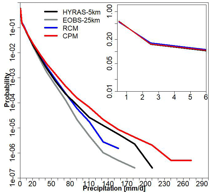
Figure 5 Empirical probability distribution functions (PDFs) of daily precipitation over SGer in the period 2000–2015 from HYRAS-5 km (black), E-OBS-25 km (grey), RCM (blue), and CPM (red). The lowest precipitation rates are shown in the upper-right corner subpanel.

The ability of CPM to represent larger precipitation rates agrees with previous literature (Ban et al., 2014; Prein et al., 2015; Fosser et al., 2014), which has been related to the enhanced intensities over orographic terrain (Langhans et al., 2012; Vanden-Broucke et al., 2018; Ban et al., 2021). The comparison against HYRAS-5 km (black) shows a good agreement by RCM and CPM for values between 1 and 50 mm d⁻¹. However, CPM (red) overestimates heavy precipitation for grid point maxima. This is a well-known deficit (Kendon et al., 2012; Berthou et al., 2018). It should also be noted that even for grid resolutions down to 1 km the updrafts might not be simulated with the right intensity, which can help explain the overestimation of precipitation at these high resolutions (Vergara-Temprado et al., 2020). It is also worth noting that the comparison against observations can suffer from under-catchment viewpoint, as the misplacement of the heavy precipitation can lead to strong local reductions, reaching even 58 % in the worst scenarios (Vergara-Temprado et al., 2020). Furthermore, problems associated with the gridding of precipitation observations and the fact that rain gauges in the Alpine region tend to be located at the valleys add uncertainty to the estimation of precipitation.

To further assess the performance of COSMO-CLM in representing precipitation extremes, we analyse the detection capability of RCM and CPM by means of a dot diagram, showing the 500 most severe events detected with the PSI in the period 1971–2015 over SGer in Fig. 6. The CPM dataset is extended to 1971 with the aid of the KLIWA-2.8 km simulation that has a similar horizontal resolution (2.8 km) and is obtained using the same model (CCLM). However, inconsistencies exist between CPM and KLIWA-2.8 km (refer to Sect. 2.2 for further details). We use HYRAS-5 km (black circles) and E-OBS-25 km (grey squares) as reference.

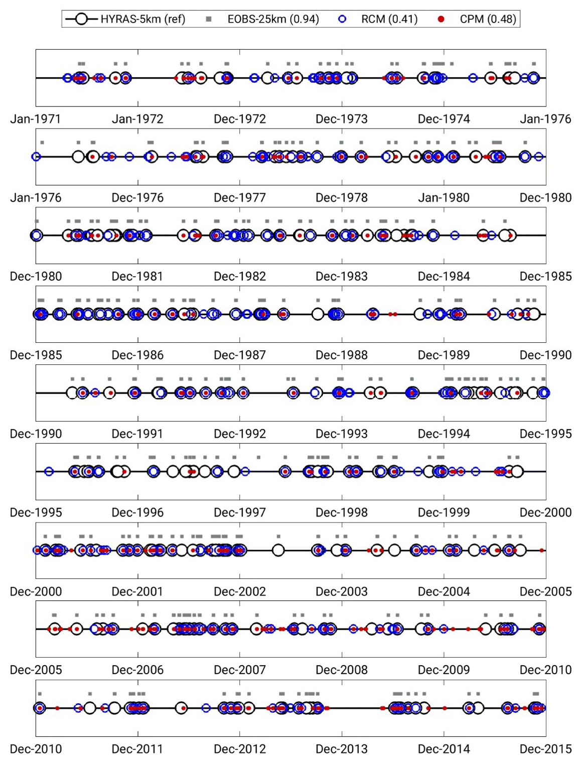
Figure 6 Dot diagram of the period 1971–2015 showing the 500 most severe precipitation events, detected using the PSI for HYRAS-5 km (black circles), E-OBS-25 km (grey squares), RCM (blue circles), and CPM (red dots). The CPM dataset is extended from January 1971 to December 1999 using KLIWA-2.8 km (Sect. 2.2). The spearman's rank correlation of the datasets is shown in the legend, where HYRAS-5 km is taken as the reference.

CPM (red dots) showed a higher spearman's rank correlation (0.48) than RCM (blue circles; 0.41), as shown in the legend of Fig. 6. Likewise, CPM outperforms RCM with regards to hit rate (number of hits divided by number of occurrences), with values of 47.2 % for CPM and 45.88 % for RCM (not shown). The rank correlations of both resolutions remain below 0.5, given the difficulty of exactly represent the same 500 events in a 44-year climatology representing 3 % of all considered days. Figure 6 also allows for observing relevant periods of heavy precipitation clustering, e.g. spring–summer of 1971, winter 1989, the years 2000 to 2002, and autumn 2013. Finally, E-OBS-25 km (grey squares) has a rank correlation of 0.94 against HYRAS-5 km, indicating a good accuracy for this product.

4 Event-scale evaluation

In the previous section, we assessed an overestimation of grid-point heavy precipitation for the convection-permitting simulation CPM but a reliable performance in detecting severe precipitation events in a 44-year climatology. Here we evaluate the performance of CPM at the event scale validating eight events. We focus on the period 2000–2015 and the investigation area CPM (Fig. 1).

Table 3 shows eight events selected using the PSI, which were also included in the derivation of the synoptic weather types in Sect. 3. Table 3 provides information about the duration of the events, the observed total precipitation, maximum grid point intensities, percentage of affected area (percentage of grid points with precipitation over the 80th percentile), severity (PSI), and associated weather types (WTs). We subjectively shortlisted the events not only to consider those events with large severity (PSI) but also to have sufficient winter and summer cases, which led to the consideration of two events with daily totals below 120 mm d⁻¹, namely 3 November 2002 and 8 July 2014.

4.1 Precipitation

We focus on two aspects of heavy precipitation, (1) amount, calculated as aggregated precipitation in time and space, and (2) structure, validated by means of the FSS metric (Sect. 2.3.3). For both metrics, we use MSWEP-11 km (Table 1) as the observational reference after coarse graining all compared datasets to a common grid of 25 km. MSWEP-11 km is used provided its high accuracy due to the inclusion of rain gauges (Beck et al., 2017) and since precipitation occurs to a large extent over the Mediterranean Sea, where HYRAS-5 km and E-OBS-25 km have no coverage.

Table 4 shows the relative differences in precipitation amount aggregated in space and time between the model and observations as ${\mathrm{RR}}_{\mathrm{rel}.\mathrm{diff}}=(\mathrm{MOD}-\mathrm{OBS})/\mathrm{OBS}$. CPM performed better than RCM in six out of the eight selected cases for precipitation amount. The largest improvement occurred for the 31 May 2013 event, which corresponds to the synoptic pattern S1 associated with the occurrence of ECOs and the advection of south-westerly moisture (Fig. 4). Using CPM brought larger precipitation rates, in agreement with the findings of Sect. 4, allowing for better scores of aggregated precipitations.

Table 4 Relative differences of spatially and temporally aggregated precipitation (${\mathrm{RR}}_{\mathrm{rel}.\mathrm{diff}.}$) between the model and observations for the duration of each event (see Table 3), calculated as ${\mathrm{RR}}_{\mathrm{mod}}-{\mathrm{RR}}_{\mathrm{obs}}/{\mathrm{RR}}_{\mathrm{obs}}$. The negative signs imply an underestimation of precipitation in the model. FSS is the fractions skill score between the model and the observations (Sect. 2.3.3). MSWEP-11 km is used as reference. The best scores are shown for FSS values closer to 1.

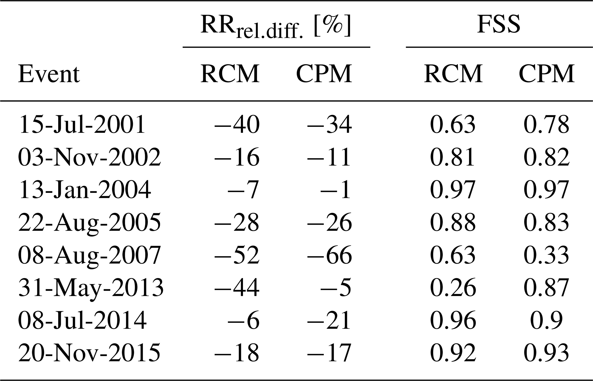
Regarding structure, CPM performed well in seven out of eight events, with FSS reaching values over 0.7. RCM, for its part, performed well for five out of eight events (Table 4). The 31 May 2013 event is again an example of good performance by CPM, where the FSS scores reached 0.87 in CPM (0.26 in RCM). The main reason for this improvement was the ability of CPM to represent larger precipitation structures over the Alps in a better agreement with MSWEP-11 km. The spatial distributions of precipitation by RCM, CPM, and MSWEP-11 km are shown in Fig. S2.

Only the event on 8 August 2007 showed a deficient performance by CPM, both for precipitation amount and structure. This event occurred under a S1 synoptic situation associated with an elongated troughs or cutoff lows (Fig. 4). The reason behind is the large underestimation of precipitation in CPM, which also hampers the structure representation.

Overall, these results showed that CPM outperforms RCM in the representation of precipitation amount and structure. The advantage of CPM lies in the better location of orographic precipitation and the larger precipitation intensities.

4.2 Humidity and temperature

In addition to precipitation errors, temperature and humidity biases could affect our interpretation of the model differences between RCM and CPM. To reduce uncertainty, we validate specific humidity (hus) and temperature (ta) profiles from RCM and CPM against radiosondes from the University of Wyoming (UWYO) and surface relative humidity (hurs) against E-OBS-25 km for the eight selected events (see Table 3).

Figure 7 shows the temporal mean bias (MB; thick line), the standard deviation of the differences (shaded area), and the root mean square errors (RMSEs; dashed line) of specific humidity (Fig. 7a) and temperature (Fig. 7b). The model output is interpolated to the location of 11 sounding stations, which were selected to have sufficient availability and fulfil the condition of a surface height difference not larger than 50 m. This requirement is introduced to avoid including large humidity and temperature biases from differences in surface topography between the model and the observations. We include all available soundings during the duration of the eight events (Table 3) in the calculation, with a temporal resolution between 6 and 12 h.

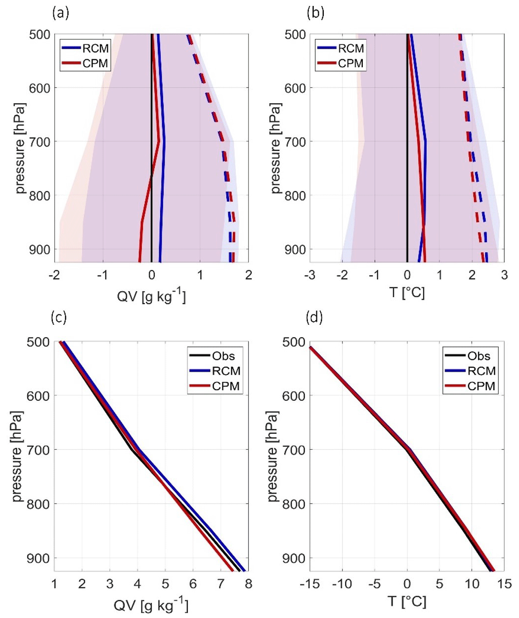
Figure 7 (a, b) Mean bias (solid line), standard deviation of the differences (shaded areas), and RMSE (dashed lines). (c, d) Humidity and temperature profiles of RCM, CPM, and the observations. Radiosondes obtained from the UWYO soundings at Nîmes (France); Oppin, Meiningen, Idar-Oberstein, Stuttgart, Kümmersbruck, and Munich (Germany); Praha (Czech Republic); and Milano, S. Pietro, and Pratica di Mare (Italy). The model information is interpolated to the station location.

Humidity is slightly overestimated by RCM throughout the whole profile and by CPM above 800 hPa (Fig. 7a). The overestimation by both models reaches 0.2 g kg⁻¹ at 700 hPa. Below 800 hPa, CPM, reduces the mean bias, reaching −0.1 g kg⁻¹, indicating a generally drier planetary boundary layer. RMSE values are similar for both simulations, being close to 1.5 g kg⁻¹ below 700 hPa. These results are promising for COSMO-CLM, since RCM and CPM show small biases even if they do not have an active data assimilation scheme and whence the model is exclusively constrained by the boundary conditions of the forcing data (ERA-Interim).

Regarding temperature (Fig. 7b), COSMO-CLM shows a warm bias, reaching 0.5 ^∘C at the 925 hPa layer for both resolutions. RMSE (Fig. 7b, dashed line) is remarkably similar between both simulations, above 2 ^∘C, with a slight improvement by CPM (red).

The humidity (Fig. 7c) and temperature (Fig. 7d) profiles show a wetter mid-troposphere (between 700 and 925 hPa) in RCM than in CPM and a similar temperature profile between both simulations, with a good agreement against observations. CPM simulates the vertical humidity profile slightly better than RCM, with a steeper humidity–height gradient. This was also observed in earlier studies with COSMO and COSMO-CLM (Caldas-Alvarez and Khodayar, 2020; Caldas-Alvarez et al., 2021). COSMO-CLM compensates for the modelling errors, simulating a wetter lower troposphere in RCM to help activate the deep-convection parameterization scheme (Tiedtke, 1989). Being of the low-level control type, the Tiedtke deep-convection scheme requires a sufficient moisture amount below the cloud base to initiate convection (Doms et al., 2013). By doing so, RCM simulates precipitation totals of the same order as CPM that rely more upon the intensification of vertical wind speeds. Furthermore, the higher humidity in the mid-troposphere helps reduce the simulated dry-air entrainment, increasing the total simulated precipitation. Both simulations show a reliable performance considering the decadal timescales

Provided the observations available below 925 hPa in the UWYO soundings were scarce, we employ the gridded E-OBS-25 km dataset (Table 1) to investigate the COSMO-CLM biases at the surface (Fig. 8). We represent the spatial distribution of temporal mean bias (colour shading) and the temporally spatially averaged mean bias and RMSE of daily surface relative humidity. We calculate relative humidity biases for this validation, given no surface-specific humidity gridded observations with sufficient accuracy were available for our region and period of investigation.

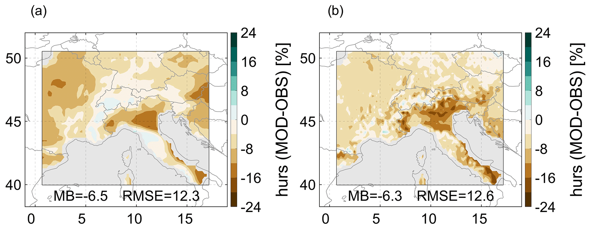
Figure 8 Spatial distributions of the surface specific humidity mean bias (MB), obtained as differences between (a) RCM and E-OBS-25 km and (b) CPM and E-OBS-25 km. All datasets have been coarse-grained to a 25 km resolution common grid. The spatially averaged MB and root mean squared error (RMSE) is shown in the text.

COSMO-CLM underestimates surface relative humidity for both RCM (Fig. 8a) and CPM (Fig. 8b), which is consistent with the well-known dry and hot bias of CPMs, provided our selected events occur mostly in summer. This is especially so at the Po Valley (Italy) and the southern Italian Peninsula. However, CPM (Fig. 8b) slightly improves the surface relative humidity deficit at locations north of the Alps, e.g. north-western France, the Czech Republic, and western Austria. These corrections in the north-western part of the simulation domain reduce the temporal and spatial MB by 3 %. However, provided the larger spatial variability of this variable in CPM due to the better orography representation, the RMSE is worsened by 5 %.

The profile and surface humidity and temperature validation have shown that (a) COSMO-CLM performs well in simulating the humidity and temperature lapse rates, albeit small biases up to 0.2 g kg⁻¹ in humidity and 0.5 ^∘C (warm bias) in temperature exist; (b) CPM simulates slightly better the vertical humidity profile with a steeper gradient than RCM; and (c) CPM reduces the positive surface relative humidity bias over locations north of the Alps, e.g. western France, the Czech Republic, and eastern Austria.

5 Main modes of heavy precipitation variability in RCM and CPM

To understand where RCM and CPM represent the main spatial patterns of heavy precipitation differently, we use PCA (Sect. 2.3.2) on events detected in HYRAS-5 km in the period 2000–2015. We do this to observe differences in the spatial distributions of heavy precipitation during the most frequent precipitation modes and reduce the dimensionality of the dataset. We combine the severe events into one set and apply PCA to obtain the EOFs and their corresponding spatial distributions. We do this separately for winter (SONDJF) and summer (MAMJJA) events for both RCM and CPM, using days above the 90th percentile of daily PSI values. In total, 290 events per season are considered to derive the EOF maps shown in Figs. 9 and S3. For this analysis, we focus exclusively on precipitation EOFs with a similar structure between RCM and CPM, dismissing the remainder of EOFs. This is done to ensure we compare model differences in similarly simulated meteorological situations.

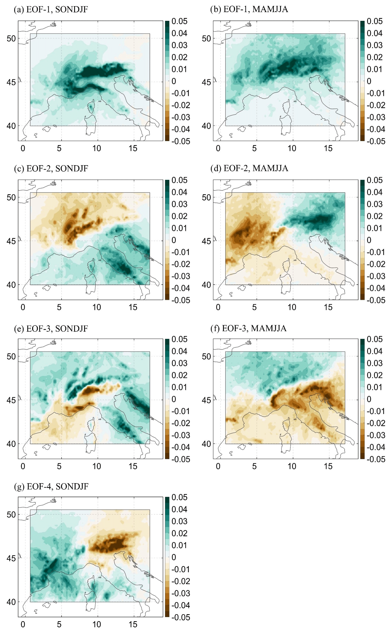
Figure 9 Empirical orthogonal functions of precipitation for SONDJF (a, c, e, g) and MAMJJA (b, d, f) events in CPM. The EOFs are obtained using the 290 most severe heavy precipitation events in each season (90th percentile).

Figure 9 shows the four leading EOF maps for winter events (Fig. 9a, c, e, and g) and the three leading modes in summer (Fig. 9b, d, and f) as simulated by CPM. The corresponding figures for RCM can be found in the SM (Fig. S3). Only CPM is shown here due to the large similarity in the spatial distributions of these EOFs with RCM. The PCA determines that the precipitation EOFs start to differ substantially between RCM and CPM after the leading four EOFs in winter and the third in summer. The four leading EOFs in winter explain 48 % of the variability for RCM and 47 % for CPM, with the first mode being the most frequent one (22 % of cases). For summer events the three leading modes of precipitation stand for 37 % of the situations in RCM and 33 % in CPM.

The visual inspection of the first EOF for winter events (Fig. 9a) shows that this the mode associated with orographic precipitation over the Alps and the northern Apennines in the Genoa region. EOF-2 (Fig. 9c) for its part shows precipitation either affecting continental Europe, north of the Alps (negative mode; brown), or affecting the Mediterranean, including the Italian and Balkan peninsulas with a marked orographic signal (positive mode; green). EOF-3 (Fig. 9e) combines precipitation over northern Europe with Mediterranean precipitation in its positive mode (green). The negative mode (brown) affects the southern Mediterranean basin between Italy and France as well as the southern and Maritime Alps. Finally, EOF-4 (Fig. 9g) shows a positive mode associated with precipitation over the Gulf of Lyons, the Balearic Sea, and the Pyrenees (green) and a negative mode affecting north-eastern Italy (brown). The latter situations of heavy precipitation in the Mediterranean have been studied in detail in the HyMeX project (Khodayar et al., 2021).

The first EOF for summer events (Fig. 9b) is associated with orographic precipitation over the Alpine region, similarly to winter EOF-1, albeit affecting parts of northern Europe, where convection can trigger more easily during the summer months. EOF-2 (Fig. 9d) shows a similar pattern to winter EOF-4 (Fig. 9g), and summer EOF-3 (Fig. 9f) shows a pattern similar to winter EOF-2 (Fig. 9c).

To summarize, RCM and CPM simulate similarly the main precipitation modes up to the fourth principal component in winter and the third in summer. These precipitation modes account for 47 % of the precipitation variability in winter and 37 % in summer, implying that the remainder of precipitation variance shows remarkable differences between RCM and CPM.

6 Model differences between RCM and CPM using composites

To further analyse model differences between RCM and CPM, we derive composites of model variables from each EOF in Fig. 9. We focus on model variables influencing the simulation of heavy precipitation, e.g. integrated water vapour (IWV), CAPE, soil–atmosphere heat fluxes, etc. To derive the composites, we select the days where daily precipitation showed the largest resemblance to the positive and negative modes of the precipitation EOFs. In other words, we select the days showing the largest positive (negative) correlations to the positive (negative) modes of each precipitation EOF. This is done separately for RCM and CPM, selecting the days with positive and negative correlations larger than 1 standard deviation of the full set. This leads to composites of ca. 30 d per positive and negative mode. We then average in time the spatial distribution of the selected days and obtain maps of the differences between RCM and CPM, as in Fig. 10. For heavy precipitation differences, we work with composites of the days assigned to each EOF, whereas for other model variables, we use the day prior to heavy precipitation. This done to study the model differences in the pre-conditioning of the event.

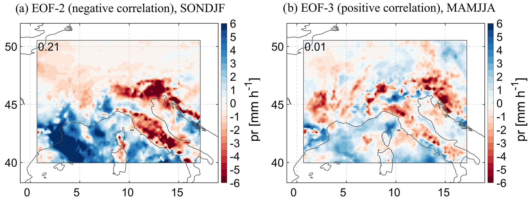
Figure 10 Composite precipitation differences between RCM (blue, positive) and CPM (red, negative). The spatial average is shown in the upper left corner. (a) Composites derived using the heavy precipitation days, with the largest negative correlation with winter (SONDJF) EOF-2 (Fig. 9c). (b) Composites derived using the heavy precipitation days, with the largest negative correlation with summer (MAMJJA) EOF-3 (Fig. 9f).

6.1 Heavy precipitation

The composites show relevant differences in precipitation amount (up to 8.5 mm h⁻¹, i.e. 204 mm d⁻¹) between RCM and CPM throughout the complete greater Alpine domain, irrespective of the simulation and meteorological situation. Spatially averaged, both RCM and CPM can represent higher precipitation than their counterpart; however, in summer, CPM represents larger precipitation at the mountain tops, e.g. the Alps and the Apennines. This holds for all analysed EOFs and both positive and negative correlations of the principal components. For illustration, Fig. 10a shows the composite differences of the negative principal components of EOF-2 in winter. Differences of up to 6 mm h⁻¹ are located east of the Spanish coast (RCM, blue), over the Apennines (Italy), and over the eastern and the Dinaric Alps (CPM, red). Spatially averaged, RCM simulates larger precipitation (0.21 mm h⁻¹) for this EOF. Figure 10b shows the positive principal components of EOF-3 in summer, where again CPM simulates larger precipitation than RCM over the Apennines (Italy), the Dinaric Alps (Balkans), and to a lower extent over the western Alps (Switzerland) and the Massif Central (France). All remainder composites are included in the SM.

These results highlight that RCM and CPM can simulate comparable precipitation amounts in the timely averages of daily precipitation (for the investigated EOFs). Regarding the larger precipitation amounts simulated by CPM over the mountain ranges, a plausible explanation is the intensification of vertical winds observed in previous studies comparing horizontal resolutions (e.g. Langhans et al., 2012; Barthlott and Hoose, 2015; Vergara-Temprado et al., 2020). Another explanation is provided by Vergara-Temprado et al. (2020), addressing that the “increase in precipitation with resolution could be happening as smaller grid boxes are easier to reach saturation”. However, the presented analysis does not allow splitting the contributions from resolution increase from other factors, e.g. changes in the physics or physical parameterizations (see Sect. 2.2).

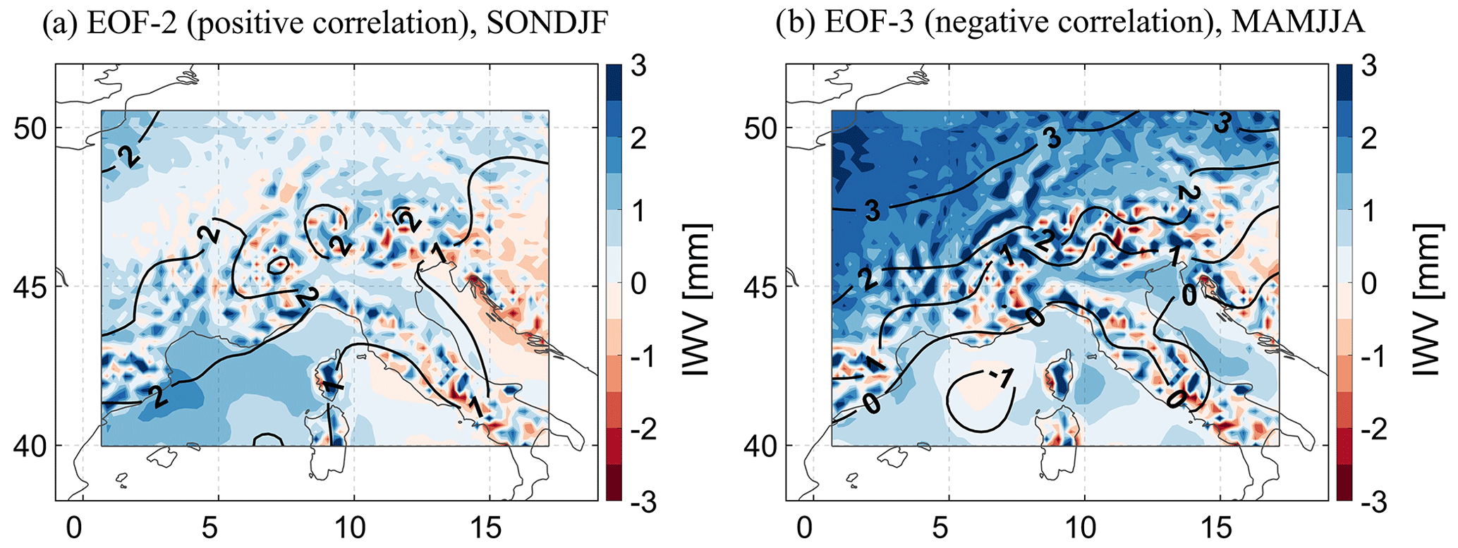
Figure 11 As Fig. 10 but for composite integrated water vapour (IWV) and ${\mathit{\theta }}_{\mathrm{e}}^{\mathrm{850}}$ differences between RCM (blue, positive) and CPM (red, negative). The IWV differences are shown in a colour shading and the ${\mathit{\theta }}_{\mathrm{e}}^{\mathrm{850}}$ differences as contours. (a) Extended winter (SONDJF) and negative correlation of EOF-2 (Fig. 9c); (b) extended summer (MAMJJA) and positive correlation of EOF-3 (Fig. 9f).

6.2 Integrated water vapour (IWV) and equivalent potential temperature at 850 hPa (${\mathit{\theta }}_{\mathrm{e}}^{\mathrm{850}}$)

Two variables typically regarded as precursors of heavy precipitation are IWV and ${\mathit{\theta }}_{\mathrm{e}}^{\mathrm{850}}$ (Doswell et al., 1996; Stucki et al., 2012). The differences of the composites show larger IWV in RCM compared to CPM throughout the whole greater Alpine region in all analysed EOFs. The IWV differences can be as large as 2 mm and take place especially over the Mediterranean Sea and the Po Valley. ${\mathit{\theta }}_{\mathrm{e}}^{\mathrm{850}}$ shows differences up to 4 K more in RCM compared to CPM. Atmospheric water vapour is the main precursor of the ${\mathit{\theta }}_{\mathrm{e}}^{\mathrm{850}}$ differences, as RCM is wetter than CPM in the 850 hPa level (Fig. 7). For illustration, Fig. 11 shows the composite differences of IWV (colour shading) and ${\mathit{\theta }}_{\mathrm{e}}^{\mathrm{850}}$ (contours) for the same principal components as Fig. 10. The composites show IWV differences up to 1 mm over the Mediterranean Sea and up to 2 K for ${\mathit{\theta }}_{\mathrm{e}}^{\mathrm{850}}$ (Fig. 11a). Likewise, the negative principal components of EOF-3 show IWV differences up to 3 mm over France and 3 K differences in ${\mathit{\theta }}_{\mathrm{e}}^{\mathrm{850}}$ by RCM (blue; Fig. 11b). The remainder composites can be found in the SM.

6.3 Soil–atmosphere interactions

Regarding variables such as surface heat fluxes, surface humidity and temperature, CAPE, and outgoing longwave radiation (OLWR), we find that CPM simulates larger outbound latent heat emissions than RCM over land but that RCM represents larger latent heat fluxes than CPM over the sea (up to 15 W m⁻²). These differences cause CPM to simulate larger near-surface specific humidity than RCM over land from northern Europe down to the Alpine barrier. South of the Alps and over the Mediterranean Sea, the opposite occurs, and RCM simulates generally wetter near-surface conditions with differences up to 1 g kg⁻¹. An example of these model responses is illustrated in Fig. 12a and c for the positive principal components of summer EOF-2 (Fig. 9d). Provided the larger surface specific humidity simulated in CPM, north of the Alps, CAPE is also larger compared to RCM due to its relationship between close-to-ground moisture (Fig. 12e).

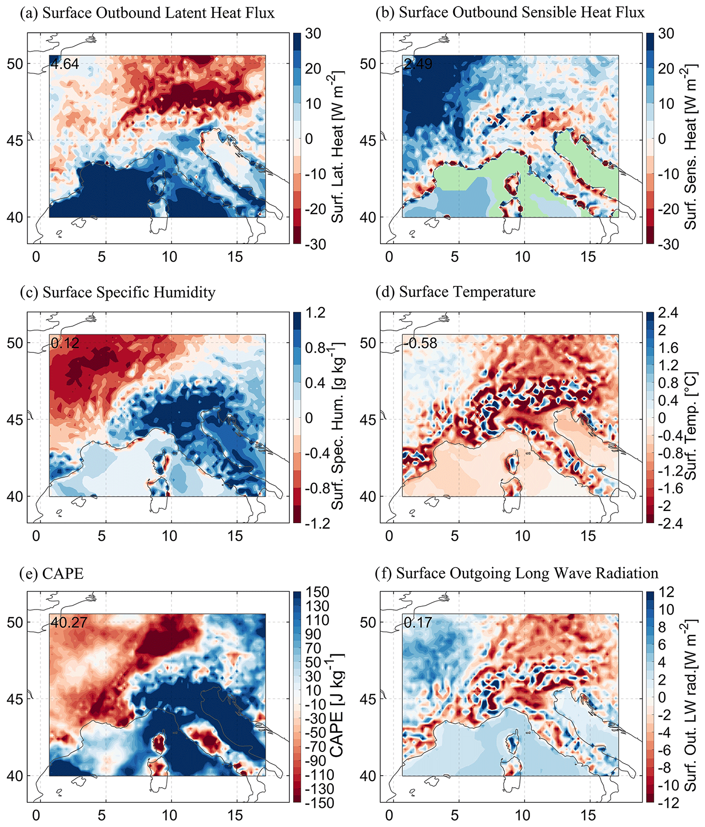
Figure 12 Composite precipitation differences between RCM (blue, positive) and CPM (red, negative). All composites correspond to the positive principal components of EOF-2 in summer (MAMJJA) events. The spatial average is shown in the upper left corner. (a) Surface outbound latent heat flux, (b) surface outbound sensible heat flux, (c) surface specific humidity, (d) surface temperature, (e) CAPE, and (f) surface outgoing longwave radiation. Green colours in latent and sensible heat fluxes denote inbound directed fluxes and are thus not shown.

Analogue to the latent heat, sensible heat fluxes show relevant differences, with RCM emitting up to 20 W m⁻² more than CPM over land, especially in summer (Fig. 12b). This causes surface temperature to be larger in RCM than in CPM (up to 1.3 ^∘C), although exceptions exist, as is the case of the composites of summer EOF-2 shown in Fig. 9d. Finally, the temperature differences close to the surface influence OLWR, whereby RCM emits larger OLWR than CPM for most of the analysed modes and their corresponding composites. Fig. 12f is however an exception, with CPM emitting larger OLWR. All composite plots can be found in the SM.

In general, the previous results hold for both summer and winter events. However, CPM emits larger latent heat flux than RCM over all land areas during winter. Also, it is worth noting that the surface temperature differences are weaker in the southern part of the domain, e.g. over Italy and the Po Valley, where CPM can show higher surface temperature. These signals cannot be attributed to severe precipitation regimes exclusively, as they were present in the seasonal means for IWV, surface temperature and humidity, and outbound latent and sensible heat flux (see Figs. S16 and S17). Finally, we would like to emphasize that our analytical approach does not allow us to relate the soil–atmosphere differences between RCM and CPM with the observed precipitation differences of Sect. 7.1.

7 Conclusions

The recent advancements in convection-permitting modelling (CPM; horizontal resolution below ca. 4 km) have been of pivotal relevance for the understanding and simulation of heavy precipitation at decadal timescales. These events with high impact are projected to be more intense and frequent in a warming climate. Therefore, despite the improvements already assessed, further research is needed to understand the implications of reaching CPM in the simulation of precipitation formation processes. In this study we evaluated reanalysis-driven COSMO-CLM simulations for the greater Alpine region over the 2000–2015 period and assessed the differences between a regional climate model (RCM) setup (grid size 25 km) and a CPM setup (grid size 3 km). The main results are presented below.

CPM represents larger precipitation intensities, a better rank correlation, better hit rates for extremes detection, and a better representation of precipitation amount and structure for selected heavy episodes than RCM. However, CPM overestimates the heaviest intensities compared to observations (also observed in Kendon et al., 2012, and Berthou et al., 2018).

The new implementation of the precipitation severity index (PSI), including a persistence parameter, proved useful for event detection in decadal datasets. Its main advantages are its flexibility to account for precipitation persistence and to allow for definition of an intensity threshold. Including these two parameters favours the ranking of longer-lasted and rarer events, whereas setting them to zero leads to a normal spatial averaging of daily precipitation.

Principal component analysis showed that winter heavy precipitation events during 1971–2015 in the greater Alpine area occur either under stationary-front situations with polar low pressure descending to the mid-latitudes or under strong north–south gradients of the 500 hPa geopotential height with a zonal flow. Four principal weather types suffice to explain most of the natural variability of winter cases. Summer events are associated with either frontal convection on the western sector of elongated upper-level troughs and evolved cutoff lows or due to winter-like synoptic patterns of stationary fronts over central Europe or strong zonal flows. Five PCs are enough to explain the natural variability of summer cases.

Principal component analysis revealed that the leading modes of the analysed heavy precipitation events start to differ between RCM and CPM after the fourth leading mode in winter (47 % of cases) and the third leading mode in summer (33 % of cases). This implies that more than half of severe precipitation events are represented differently in RCM and CPM and thus the choice of modelling approach is crucial, especially for summer cases. Composite maps derived from the leading modes showed that CPM systematically represents more precipitation at the mountain tops but that RCM may show large intensities (up to 200 mm d⁻¹) in other regions.

RCM represents larger integrated water vapour than CPM, especially over the Mediterranean Sea and the Italian Peninsula in the pre-conditioning of summer events (up to 2 mm). The larger moisture in RCM comes from an intensified latent heat flux emission over the sea and a wetter, lower free troposphere. This was validated for eight selected reprecipitation events against radiosondes. As a result, equivalent potential temperature at the 850 hPa level was also systematically larger in RCM than in CPM (up to 3 K).

At the ground level, CPM simulates larger latent heat flux over land than RCM (up to 15 W m⁻²) on the day prior to severe precipitation. This occurs both for summer and winter composites, although in summer this effect is constrained to areas north of the Alps. Over the sea, the opposite occurs, and RCM simulates larger latent heat fluxes compared to CPM (30 W m⁻²). The consequence is a wetter surface level (1 g kg⁻¹ specific humidity) and larger CAPE (140 J kg⁻¹) in CPM north of the Alps and a wetter surface level in RCM over the Mediterranean Sea and Italy, possibly associated with the southerly Mediterranean winds. In turn, RCM simulates larger sensible heat fluxes over land, which leads to a generally hotter surface level than in CPM (by about 1.5 ^∘C). These differences are weaker to the south of the Po Valley. Finally, the higher temperatures over land in RCM bring larger emissions of outgoing longwave radiation compared to CPM (9 W m⁻²).

It is worth mentioning that for variables such as surface-specific humidity and temperature, or surface heat fluxes, the signal of the differences between RCM and CPM was already present in the seasonal means (Figs. S16 and S17). This implies that they are not exclusive of heavy precipitation situations but that they could be present in other weather regimes. For instance, the fact that CPM represents a higher temperature at the Po Valley in the summer adds on to the findings by Sangelantoni et al. (2023), where an amplification of heat waves over the same area was found in a CPM ensemble.

Our study has limitations that need to be briefly addressed. First, we only assess one regional climate model, and hence our results cannot be generalized to other RCMs. Second, as is common in heavy precipitation studies the under-catchment problem might be present in the observations used for validation (Groisman and Legates, 1994; Golubev, 1986; Goodison et al., 1997; Vergarara-Temprado et al., 2020). Finally, we would like to point out that our study compares two different simulations, where the differences observed are due to the use of a different horizontal resolution (25 km vs. 3 km) but also to the different fine tuning of the settings and the different boundary data.

Notwithstanding these limitations, our study provides evidence of the added value of CPM and of the remarkable differences existing between RCM and CPM. These systematic differences must be considered when using one setup or the other in decadal simulations. This is relevant for future research in the field but also for third parties interested in using climate information at decadal timescales. Examples of endeavours where high-resolution climate data are bringing added value are, for instance, the downscaling of climate change projections (Pichelli et al., 2021), the development of decision-relevant strategies for climate change adaptation (BMBF-RegIKlim), or their use in forestry or hydrology applications.