the Creative Commons Attribution 4.0 License.
the Creative Commons Attribution 4.0 License.
 | 18 Jul 2023
The role of boundary layer processes in summer-time Arctic cyclones
Hannah L. Croad
John Methven
Ben Harvey
Sarah P. E. Keeley
Ambrogio Volonté
Arctic cyclones are the most energetic weather systems in the Arctic, producing strong winds and precipitation that present major weather hazards. In summer, when the sea ice cover is reduced and more mobile, Arctic cyclones can have large impacts on ocean waves and sea ice. While the development of mid-latitude cyclones is known to be dependent on boundary layer (BL) turbulent fluxes, the dynamics of summer-time Arctic cyclones and their dependence on surface exchange processes have not been investigated. The purpose of this study is to characterise the BL processes acting in summer-time Arctic cyclones and understand their influence on cyclone evolution. The study focuses on two cyclone case studies, each characterised by a different structure during growth in the Arctic: (A) low-level-dominant vorticity (warm-core) structure and (B) upper-level-dominant vorticity (cold-core) structure, linked with a tropopause polar vortex. A potential vorticity (PV) framework is used to diagnose the BL processes in model runs from the ECMWF Integrated Forecasting System model. Both cyclones are associated with frictional Ekman pumping and downward sensible heat fluxes over sea ice. However, a third process, the frictional baroclinic generation of PV, acts differently in A and B due to differences in their low-level temperature structures. Positive PV is generated in Cyclone A near the bent-back warm front, like in typical mid-latitude cyclones. However, the same process produces negative PV tendencies in B, shown to be a consequence of the vertically aligned axisymmetric cold-core structure. This frictional process also acts to cool the lower troposphere, reducing the warm-core anomaly in A and amplifying the cold-core anomaly in B. Both cyclones attain a vertically aligned cold-core structure that persists for several days after maximum intensity, which is consistent with cooling from frictional Ekman pumping, frictional baroclinic PV generation, and downward sensible heat fluxes. This may help to explain the longevity of isolated cold-core Arctic cyclones with columnar vorticity structure.
- Article
(11451 KB) - Full-text XML
- BibTeX
- EndNote


The rapid loss of sea ice due to anthropogenic global warming (e.g. Comiso, 2012; Meier et al., 2014) is permitting human activity to expand into the summer-time Arctic. For example, reduced sea ice extent and thickness will open up shorter shipping routes through the Arctic between Atlantic and Pacific ports (Melia et al., 2016). This human activity will be exposed to the risks of Arctic weather during the summer, including Arctic cyclones.
Arctic cyclones are synoptic-scale low-pressure systems developing, or moving into, the Arctic. They produce some of the most impactful weather in the Arctic, with strong winds at the surface and sometimes extreme ocean waves (e.g. Thomson and Rogers, 2014; Waseda et al., 2018). Arctic cyclones are also associated with atmospheric forcings that have large impacts on the sea ice (e.g. Simmonds and Keay, 2009; Asplin et al., 2012; Zhang et al., 2013; Peng et al., 2021). As the climate warms the summer-time Arctic is becoming increasingly dominated by the marginal ice zone (MIZ; Strong and Rigor, 2013), a band of fragmented ice floes separating the ice-free ocean and the main ice pack. In recent years the MIZ has widened by 39 % (Strong and Rigor, 2013) in summer, with MIZ fraction (MIZ extent divided by total sea ice extent) increasing by more than 50 % (Rolph et al., 2020). Thinner and more mobile ice in the MIZ will result in enhanced surface interactions with Arctic cyclones, with greater surface drag due to ice floe morphology (Lüpkes and Birnbaum, 2005; Elvidge et al., 2016), and enhanced surface sensible and latent heat fluxes due to a greater exposure of the ocean surface. For example, it has been argued that record-low sea ice extent in 2012 was exacerbated by an extremely strong cyclone, the great Arctic cyclone of 2012 (AC12; Simmonds and Rudeva, 2012), with enhanced ice melt due to increased upward ocean heat transport (Zhang et al., 2013).
Forecast skill in the Arctic is lower, but generally comparable, to that in Northern Hemisphere mid-latitudes (Jung and Matsueda, 2016; Sandu and Bauer, 2018), based on 500 hPa geopotential anomaly correlation scores. Lower predictability in the Arctic is likely related to the relative sparsity of observations there, resulting in larger uncertainties in initial conditions for numerical weather prediction models. Previous work has also demonstrated that the forecast skill of Arctic cyclones is lower than that of mid-latitude cyclones. For instance, Yamagami et al. (2018a) demonstrated that the mean predictability of 10 extraordinary Arctic cyclone cases was 2.5–4.5 d, around 1–2 d less than that of Northern Hemisphere mid-latitude cyclones (Froude, 2010). Furthermore, using ensemble forecasts, Capute and Torn (2021) demonstrated that the ensemble mean root-mean-square error and ensemble standard deviation for cyclone position was higher for 100 selected summer-time Arctic cyclones than for 89 selected winter-time Atlantic mid-latitude cyclones. Yamagami et al. (2018b) examined the predictability of AC12 and found that the position variability was greater than intensity variability between ensemble forecasts. Furthermore, ensemble members that best captured the upper-level vortex merger associated with AC12 produced the best forecasts, demonstrating that an understanding of cyclone dynamics and mechanisms is critical for predictability. Improvements in Arctic cyclone forecasting can likely be achieved through a better understanding of the physical processes that distinguish Arctic cyclones from mid-latitude cyclones, including the different growth mechanisms and interaction with sea ice.
Vessey et al. (2022) demonstrated that the composite structure of intense summer-time Arctic cyclones is distinct to that of intense winter-time Arctic and North Atlantic mid-latitude cyclones. Summer-time Arctic cyclones undergo a structural transition at the time of maximum intensity, from a tilted baroclinic system to an axisymmetric cold-core structure. The mean lifetime of the summer-time Arctic cyclones was also found to be more than 3 d greater than that of winter-time Arctic cyclones and 4 d greater than that of winter-time North Atlantic mid-latitude cyclones (Vessey et al., 2022). The longevity of some Arctic cyclones and the transition to an axisymmetric cold-core structure have also been documented in several case studies (e.g. Simmonds and Rudeva, 2012; Tanaka et al., 2012; Aizawa and Tanaka, 2016; Yamagami et al., 2017; Tao et al., 2017).
Many of the growth mechanisms of summer-time Arctic cyclones are the same for mid-latitude cyclones, such as baroclinic instability and lee cyclogenesis. However, sustained cyclone interaction with tropopause polar vortices (TPVs), long-lived vortices on the tropopause with horizontal scales of less than 1500 km (Cavallo and Hakim, 2009), is a characteristic of the Arctic (where there is typically an absence of a strong zonal jet stream in the upper troposphere). Gray et al. (2021) classified Arctic cyclones as being either (i) “unmatched” and (ii) “matched” with a TPV during development, using a statistical matching criterion based on a threshold distance between tracked TPVs and low-level cyclones. It was found that unmatched cyclones are initially dominated by low-level vorticity such that vorticity decreases with height. These cyclones occur most commonly along the northern coast of Eurasia (Fig. 7 in Gray et al., 2021), in association with high baroclinicity on the Arctic frontal zone (AFZ; Serreze et al., 2001; Day and Hodges, 2018). In contrast, matched cyclones are dominated by upper-level vorticity (vorticity increases with height). Matched cyclones are associated with reduced tilt and baroclinicity, and a single columnar vortex structure at maximum intensity (like the summer-time Arctic cyclone composite in Vessey et al., 2022). Matched cyclones track most frequently along the North American coastline (Fig. 7 in Gray et al., 2021), consistent with the climatological location of TPVs (Cavallo and Hakim, 2010).
In this study, Arctic cyclones will be classified in terms of their vorticity structure during development as either (i) low-level dominant or (ii) upper-level dominant. Note that by thermal wind balance, these cyclones have (i) low-level warm cores (i.e. a horizontal temperature maximum) and (ii) tropospheric cold cores respectively. This is somewhat similar to the unmatched and matched classification used by Gray et al. (2021) but focuses on the vertical gradient in vorticity rather than the identification of TPVs. These classifications are based on cyclone structure at an instant, in contrast to the Petterssen and Smebye (1971) classification of type A (low-level forcing) and type B (upper-level forcing) cyclones, which describes the development mechanisms.
One of the biggest uncertainties in the modelling of Arctic cyclones is the interaction with the surface and sea ice. Turbulent fluxes of momentum, heat, and moisture in the boundary layer (BL) are critical to understanding the cyclone–sea ice interaction. It is known that BL turbulent fluxes have large impacts on the evolution of mid-latitude cyclones. Here we discuss the momentum fluxes first (sensible heat fluxes are discussed in a later paragraph). Friction acts to reduce the intensity of cyclones, with Valdes and Hoskins (1988) demonstrating that surface drag can reduce the growth rates of baroclinic systems by up to 50 %. The dominant physical mechanism responsible for this is often assumed to be Ekman pumping. In Ekman pumping, BL friction causes the near-surface wind to weaken and turn toward the low centre. The subsequent convergence forces ascent at the BL top, which acts to spin down the cyclone via barotropic vortex squashing (Sect. 8.7 in Hoskins and James, 2014, and Sect. 8.4 in Holton and Hakim, 2012).
Previous studies have used a potential vorticity (PV) framework to identify the mechanisms by which BL processes impact mid-latitude cyclones. PV is a central variable in the evolution of baroclinic systems (e.g. Hoskins et al., 1985), considering both vorticity and stratification:
where P is the Rossby–Ertel PV (K m2 kg−1 s−1), ρ is density (kg m−3), ζa is absolute vorticity (s−1), and θ is potential temperature (K). PV is materially conserved for adiabatic, inviscid motion but not in the presence of friction and diabatic heating. Lagrangian changes in PV are expected in the BL where friction and diabatic heating are important. The benefit of using a PV framework is that structural changes within a cyclone can be inferred from any changes in PV, with the constraint of thermal wind balance. A PV framework is used over an energetics framework, for example, where changes in circulation and the constraint of thermal wind balance are not transparent.
The impact of BL friction on a (barotropic) cyclonic vortex can be understood in the PV framework by following an idealised thought experiment from Sect. 17.6 in Hoskins and James (2014). Friction weakens the near-surface winds in a cyclone, reducing the azimuthal cyclone circulation (i.e. the vertical component of vorticity), and therefore reduces PV in the BL near the low centre. In a balanced state, there is both a reduction in cyclonic circulation and BL static stability. To achieve this, in the absence of other non-conservative processes, isentropes must rise, increasing the static stability above the BL. To conserve PV above the BL, vorticity must decrease there. This is the Ekman pumping process, characterised by a negative PV tendency in the BL, and a secondary circulation with inflow within the BL and ascent near the cyclone centre which acts to spin down vorticity in and above the BL.
The PV framework also reveals a second frictional process in mid-latitude cyclones, in which friction acts to alter horizontal vorticity and circulation in the x–z and y–z planes. This process is called “frictional baroclinic PV generation” and is most prominent in regions of strong horizontal temperature gradients where isentropes have significant tilt, such as fronts. In this process, PV is generated in the BL where surface winds oppose the tropospheric thermal wind (Cooper et al., 1992). This frictional baroclinic PV generation occurs mainly to the east and north-east of cyclone centres along the warm front (Stoelinga, 1996; Adamson et al., 2006; Plant and Belcher, 2007; Vannière et al., 2016). Boutle et al. (2007) found evidence of both Ekman pumping and baroclinic PV generation in multiple model simulations, with the relative importance of each term depending on cyclone initialisation. In baroclinic wave cyclones with strong low-level temperature gradients, baroclinic generation dominates (Adamson et al., 2006; Boutle et al., 2007). Consistent with this, Stoelinga (1996) found that BL friction generated mainly positive low-level PV in their mid-latitude cyclone modelling study. However, a sensitivity experiment showed that the overall effect of surface drag was to produce a weaker cyclone due to the reduced development of the upper-level wave (i.e. reduced baroclinicity and mutual growth of the upper and lower waves). This is consistent with the baroclinic PV mechanism described by Adamson et al. (2006), whereby positive PV generated in the BL is ventilated out of the BL by the warm conveyor belt (WCB) and advected above the low centre. This positive PV is associated with increased static stability above the BL, acting as an insulator to reduce the coupling of the upper and lower levels, reducing the cyclone growth rate. Note that both frictional Ekman pumping and the baroclinic PV mechanism have impacts above the BL (in fact Boutle et al., 2015, suggest that these processes act in union to maximise cyclone spin-down), demonstrating that the role of surface friction in a cyclone is more complicated than the simple Ekman spin-down of vorticity in a barotropic vortex.
Sensible heat fluxes have a direct effect on PV by altering static stability in the BL. For example, Chagnon et al. (2013) identified a region of negative BL PV behind the cold front of a mid-latitude cyclone, generated due to strong upward sensible heat fluxes (i.e. the surface losing heat to the overlying atmosphere), associated with reduced BL static stability. Haualand and Spengler (2020) and Bui and Spengler (2021) demonstrated that the direct effect of surface sensible heat fluxes is to weaken mid-latitude cyclone development by reducing low-level baroclinicity, using PV and energy frameworks respectively in idealised modelling setups. However, both studies found that the impact of sensible heat fluxes was relatively small compared to that of latent heating. Sensible heat fluxes also modify the action of friction by altering BL stability and by weakening frontal gradients (Plant and Belcher, 2007).
This PV framework has been used exclusively to study mid-latitude cyclones. The role of BL processes in the evolution of summer-time Arctic cyclones has not yet been investigated. Differences are expected for several reasons: (i) the sea ice surface in summer is characterised by increased surface roughness in the MIZ and variable sensible heat fluxes; (ii) there are longer-lived cyclones in the summer-time Arctic, so BL processes have a longer time to act; and (iii) there are different cyclone growth mechanisms and structures in the summer-time Arctic such that BL processes might impact cyclone evolution in different ways.
In this study we aim to answer the following questions using two case studies from summer 2020:
-
What is the nature of the BL processes acting in contrasting summer-time Arctic cyclones?
-
How does the nature of the BL processes change as the cyclones evolve?
-
What is the impact of the BL processes on Arctic cyclones outside the BL?
The paper is structured as follows. The methodology is described in Sect. 2, including the model setup employed and details of the PV framework. Section 3 describes two Arctic cyclone case studies from summer 2020. The main results are presented in Sect. 4, with a qualitative comparison to the existing literature on mid-latitude cyclones. A more general discussion is provided in Sect. 5, and the study is concluded in Sect. 6.
2.1 Reanalysis data
The study uses data from the ERA5 dataset, the fifth-generation European Centre for Medium-Range Weather Forecasts (ECMWF) reanalysis product (Hersbach et al., 2017, 2020). ERA5 was produced using the ECMWF's Integrated Forecasting System (IFS) model cycle 41r2, which was operational from 8 May to 21 November 2016. The model has spectral truncation TL639 (horizontal resolution ∼31 km) and 137 terrain-following hybrid-pressure levels from the surface to 0.01 hPa. The 6-hourly data on a 0.25∘ regular latitude–longitude grid are used to perform an analysis of Arctic cyclones from the 2020 extended summer (May–September) season.
2.2 IFS model runs
The primary tool used in the study is the ECMWF global IFS model, coupled with dynamic ocean and sea ice models. Forecasts were run using IFS model cycle 47r1, with spectral truncation O640 (horizontal resolution ∼18 km) and 91 terrain-following hybrid-pressure levels up to 0.01 hPa. This is the same setup as the control member of the ECMWF ensemble forecasting system (ENS) which was operational from 30 June 2020 to 10 May 2021. A prognostic dynamic–thermodynamic sea ice model, the Louvain-la-Neuve Ice Model (LIM version 2), is used, incorporated into the dynamical ocean model (NEMO version 3.4; Nucleus for European Modelling of the Ocean). Model runs starting at 00Z are used, with 6-hourly forecasts out to 10 d.
In this study the BL height diagnostic from the IFS model is used, which is determined using a bulk Richardson number (ECMWF, 2020). The BL top is defined as the level at which the bulk Richardson number reaches the critical value of 0.25, i.e. the level at which the flow is no longer turbulent. The surface momentum flux and surface sensible heat flux are also used directly from the IFS model and are computed using bulk formulae with exchange coefficients (ECMWF, 2020).
2.3 Arctic cyclone tracking
Tracks of Arctic cyclones are identified from ECMWF ERA5 reanalysis data and from the ECMWF IFS model runs (the control member of ENS, model cycle 47r1) using the TRACK programme developed by Hodges (1994, 1995, 2021). The TRACK algorithm is employed on the T5–63 and T5–42 filtered 850 hPa relative vorticity from ERA5 and the ENS control member respectively, identifying anomalies exceeding 10−5 s−1. Only tracks that last longer than 1 d and travel more than 1000 km are retained.
2.4 A modified cyclone phase space
A modified cyclone phase space for characterising the structure of Arctic cyclones is proposed. This phase space is based on the thermal asymmetry and thermal wind structure of a cyclone, as in Hart (2003), but is presented in a non-dimensionalised and more direct way. Thermal asymmetry is quantified here as a non-dimensionalised depth-integrated baroclinicity, B, over the 925–700 hPa layer (assumed to be above the BL but below the “steering” level). As in Hart (2003), this represents the linear variation in temperature across the cyclone (of radius 500 km) by splitting the cyclone into a right (R) and left (L) half:
where f0 is the Coriolis parameter (s−1), L is the cyclone length scale (500 km), N is the Brunt–Väisälä frequency (0.01 s−1), g is the gravitational acceleration (9.81 m s−2), θ0 is the reference potential temperature (273 K), p is pressure (hPa), and θR and θL are the areal mean potential temperatures over a semi-circle of radius 500 km to the right and left of the cyclone (K). In the Hart (2003) phase space, the cyclone is split in half by the cyclone motion vector. However, Arctic cyclones can be associated with slow movement and remain quasi-stationary for considerable periods of time such that the motion vector is not well defined. Hence, here B is calculated at every 10∘ bearing, with the maximum value of B being used at each time. The larger the value of B, the greater the asymmetry and baroclinicity of a cyclone.
Thermal wind balance can be written in terms of vorticity (Eq. 12.6 in Hoskins and James, 2014):
where ξ is relative vorticity (s−1), z is height (m), b′ is the buoyancy anomaly (, m s−2), and θ′ is the potential temperature anomaly. A system in the Northern Hemisphere where ξ increases with height (; upper-level dominant) must be in balance with a cold-core thermal wind structure (negative buoyancy anomaly), as corresponds to (since for systems of length scale L). In contrast, ξ decreases with height (low-level dominant) in warm-core systems. Hence, the thermal wind structure is quantified here as a non-dimensionalised vertical gradient of relative vorticity in the 700–400 hPa layer (assumed to be above the “steering” level but below the tropopause):
where is calculated by a linear regression fit of ξ at 50 hPa intervals between 700 and 400 hPa. The quantity RoT is the thermal Rossby number, the non-dimensional ratio of the inertial force due to the thermal wind and the Coriolis force. The form in Eq. (4) is obtained using the Burger number (, where H is the height scale), the non-dimensional ratio of the density stratification and Earth's rotation in the vertical, which is assumed to be 1 for the synoptic scale. A positive RoT indicates a low-level-dominant cyclone and therefore a warm-core structure, whilst a negative RoT corresponds to an upper-level-dominant cyclone or cold-core structure.
The circularly symmetric component of θ′ (and equivalently b′) can be expressed in terms of the potential temperature at the cyclone centre, θC, and a background potential temperature, θB (representing the average value at a 500 km radius). Making a second-order finite difference approximation – – and substituting into Eq. (4) using thermal wind balance in Eq. (3) gives
The appeal of this cyclone phase space is that it is non-dimensionalised, and it is dependent on the potential temperature structure of the cyclone only. Note that in Eqs. (2) and (5), the quantities θR−θL and θC−θB are scaled in the same way such that their magnitudes can be directly compared.
2.5 PV framework
In the presence of friction and diabatic heating, the Lagrangian evolution of PV is given by
where ρ is density (kg m−3) and F is the frictional force vector (m s−2). is the PV flux arising from non-conservative terms in the Haynes and McIntyre (1987) form. The first term on the right-hand side (RHS) of Eq. (6) represents frictional effects on PV, whilst the second term represents diabatic heating effects, which can be split into sensible (shf) and latent (lhf) heat flux contributions. Application of Eq. (6) in the BL would require full 3-D fields of friction and diabatic heating, which would be strongly dependent on the 3-D structure of parameterised tendencies and would be difficult to interpret. Therefore a simplified expression for the BL depth-averaged PV tendency was derived by Cooper et al. (1992). It is assumed that the horizontal variation in fluxes is substantially smaller than the vertical variation in the BL such that
where τ is the momentum flux, and H is the sensible heat flux. A linear flux gradient is also assumed in the BL such that fluxes can be specified as a product of their surface values, τS and HS, decreasing linearly to zero at the top of the BL with height h:
where S(Z) is a linear function of height in the BL. Note that the convention used here is that τS is taken to be in the same direction as the surface wind (i.e. τS is the stress that the atmosphere exerts on the surface). The frictional and sensible heating terms on the RHS of Eq. (6) can be decomposed into the contributions from the vertical and horizontal components in the dot products (where ∇H is the horizontal gradient operator):
where density is assumed constant (ρ=ρ0) within the BL for simplicity. Equations (7) and (8) can be substituted into Eq. (9) to give a new expression in terms of τS, HS, and the linear function of height S(z). The following depth-average operator is then applied:
With some manipulation the BL depth-averaged PV tendency equation from Cooper et al. (1992) is obtained in the form used in Vannière et al. (2016):
where subscript h refers to the top of the BL, v is the horizontal wind vector, and Δ refers to a change in quantity between the surface and the BL top. Equation (11) contains five terms, each representing a non-conservative process which gives rise to a Lagrangian tendency of PV in the BL. Note that each term in Eqs. (9) and (11) has been prescribed a shorthand name according to whether the term is associated with friction (F), sensible heat fluxes (S), or latent heat fluxes (L). Also note that no assumptions are made about PV conservation or invertibility in this derivation. Although these equations have been derived and used previously in the context of mid-latitude cyclones, the assumptions made regarding turbulent mixing are equally applicable in the Arctic.
The FEK term refers to Ekman friction, capturing the impact of friction on the vertical component of vorticity. This term is proportional to the vertical Ekman pumping and is negative for a cyclone () with a stably stratified BL (Δθ>0). The FBG term is called baroclinic PV generation, capturing the impact of friction on the horizontal components of vorticity relating to vertical wind shear. This term is proportional to the horizontal gradient of potential temperature at the BL top, so it is large in the vicinity of fronts. The sign of this term depends on the orientation of the surface stress and the thermal wind above the BL (see Sect. 5). In mid-latitude cyclones FBG is positive along the warm front where the surface winds oppose the tropospheric thermal wind (e.g. Adamson et al., 2006). The SV term refers to the impact of sensible heat fluxes on the stratification in the vertical. This term is positive for a cyclone () with downward sensible heat fluxes (HS<0). Term SH is proportional to the horizontal gradient of sensible heat fluxes. Previous studies have found this term to be negligible compared to the other terms (e.g. Plant and Belcher, 2007; Vannière et al., 2016). Term L represents the effect of latent heating, which is not discussed in this paper.
2.6 Depth-integrated PV budget
To understand how the BL PV tendencies impact cyclone evolution, depth-integrated PV budgets will be considered using control volumes centred on the cyclone. Here we consider the quantity 〈P〉, which represents the mass-weighted volume average of PV or the “amount of PV substance”, following the terminology of Haynes and McIntyre (1990):
Note that 〈P〉 equals the depth-integrated circulation around the lateral boundary of the control volume only if the top and bottom boundaries of the volume are isentropic surfaces. Since the baroclinic PV generation term depends on the gradient in potential temperature at the top of the BL (Eq. 11), when this term is strong, it is more precise to refer to 〈P〉 as PV substance than the depth-integrated circulation.
Consider an atmospheric column modelled as a cylinder centred on a cyclone, split vertically into the BL (height h) and free-tropospheric layer above. The vector normal to the BL top is , and is the outward normal to the lateral boundary of the column. The top of the free-tropospheric layer is chosen to be an isentropic surface, θtop (at height ztop=z(θtop)), near the tropopause, which ensures that there is no PV flux across it due to the impermeability theorem (Haynes and McIntyre, 1987). Here θtop=330 K is used, as this level is found to reside just above the tropopause in the summer-time Arctic. There can be PV flux across the surface between the two layers (as the BL top is not necessarily an isentropic surface), and there can be PV flux across the lateral boundary. Non-conservative processes in the BL and free troposphere are included in the formulation (although the latter are not calculated explicitly). Note that whilst non-conservative processes in the free troposphere may occur at mid-levels within Arctic cyclones, in particular latent heating, these are not the subject of this study. However, the changes in 〈P〉 diagnosed in the IFS model include the effects of all processes, including latent heat release above the BL.
Using this setup, the volume integral in Eq. (12) can be calculated following the method in Saffin et al. (2021) using Gauss' theorem and the Leibniz rule to obtain
where and are the depth-integrated PV tendencies in the BL and free-tropospheric layer respectively, u is the 3-D wind vector (m s−1), and ub is the velocity of the boundary of the control volume (m s−1). In this work we examine the left-hand side (LHS) of Eqs. (13) and (14) and the non-conservative processes in the BL (the first term on the RHS of Eq. 13). Non-conservative processes in the free troposphere (the first term on the RHS of Eq. 14), are not explicitly calculated. The second term on the RHS represents the vertical flux of PV across the surface between the two layers. If the BL top is flat, can be written as , where w is vertical velocity (m s−1) and is the rate of change of BL height (m s−1). The third term on the RHS represents the horizontal fluxes of PV across the lateral boundary. Note that, along with the non-conservative processes in the free troposphere, the vertical and horizontal fluxes of PV are not explicitly calculated here.
The 2020 extended summer (May–September) season is used as a sample of Arctic cyclones from which to identify case studies for further analysis. An analysis of the cyclones was performed using the ERA5 dataset (Fig. 1). Arctic cyclones are identified as vorticity maxima with 850 hPa relative vorticity, ξ850, greater than s−1 in the Arctic (>70∘ N) at least once along their track. From manual inspection the ξ850 constraint was found to be a good filter for distinguishing synoptic-scale Arctic cyclones from smaller-scale vorticity features.
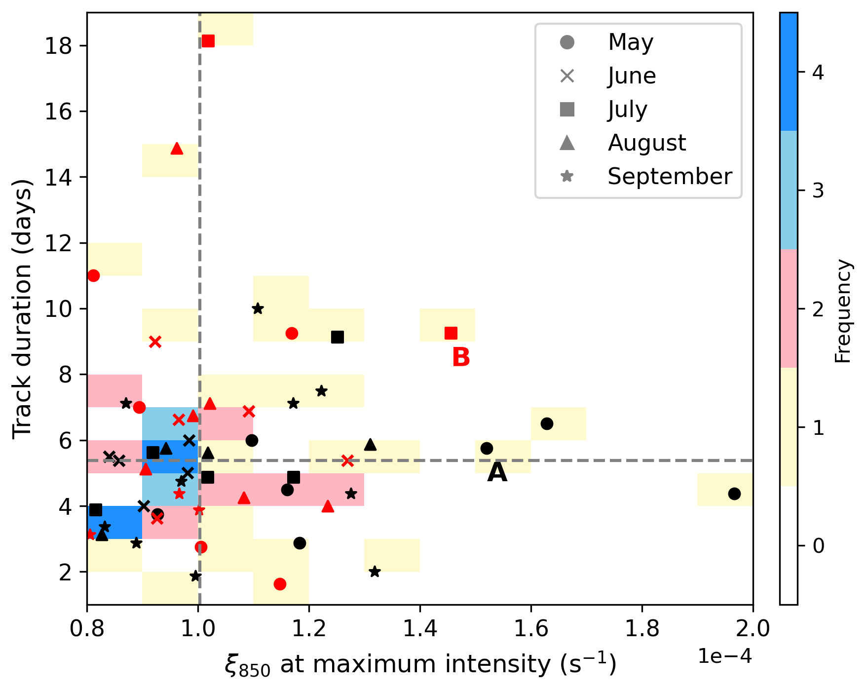
Figure 1The 2-D histogram of ξ850 at maximum intensity (x axis) and track duration (y axis) of summer 2020 Arctic cyclones from ERA5. Black and red markers refer to low-level and upper-level-dominant cyclones respectively, as diagnosed by the thermal Rossby number, RoT, from the modified cyclone phase space (Sect. 2.4) at the time of maximum growth rate. The shading illustrates the number of cyclones that populate a region of the histogram space. The median values of ξ850 at maximum intensity and track duration are demonstrated by the dashed grey lines. Cyclone cases A and B are annotated with the respective letter to the bottom right of the marker.
Using these criteria, 52 Arctic cyclone tracks were identified from the 2020 summer season. The median strength in ξ850 was s−1 at maximum intensity, and the median track duration was approximately 5.4 d (Fig. 1). In Fig. 1, Arctic cyclones are also classified as low-level dominant (RoT>0; black markers) or upper-level dominant (RoT<0; red markers), diagnosed at the time of maximum growth rate. In 2020, 60 % of the Arctic cyclones were low-level dominant (31), and 40 % were upper-level dominant (21) during development. The median track duration of the low-level-dominant cyclones was 5.13 d, whilst the upper-level-dominant cyclones had a longer median track duration of 6.75 d. The median strength at maximum intensity was similar for both sets of cyclones ( s−1).
For the purposes of this investigation two case studies are chosen, one with low-level-dominant development and the other with upper-level-dominant development. Cyclones A and B (annotated in Fig. 1) are selected as the strongest cyclones that spend a considerable amount of time over sea ice (note that the two strongest cyclones of the season were not chosen as case studies because the cyclone centres did not track over sea ice). Cyclone A (low-level-dominant development) occurred in May 2020 and was the third strongest cyclone of summer 2020 with s−1 at maximum intensity and a lifetime of almost 6 d. Cyclone B (upper-level-dominant development) was the fourth strongest cyclone with s−1 at maximum intensity, with a longer track duration of almost 10 d.
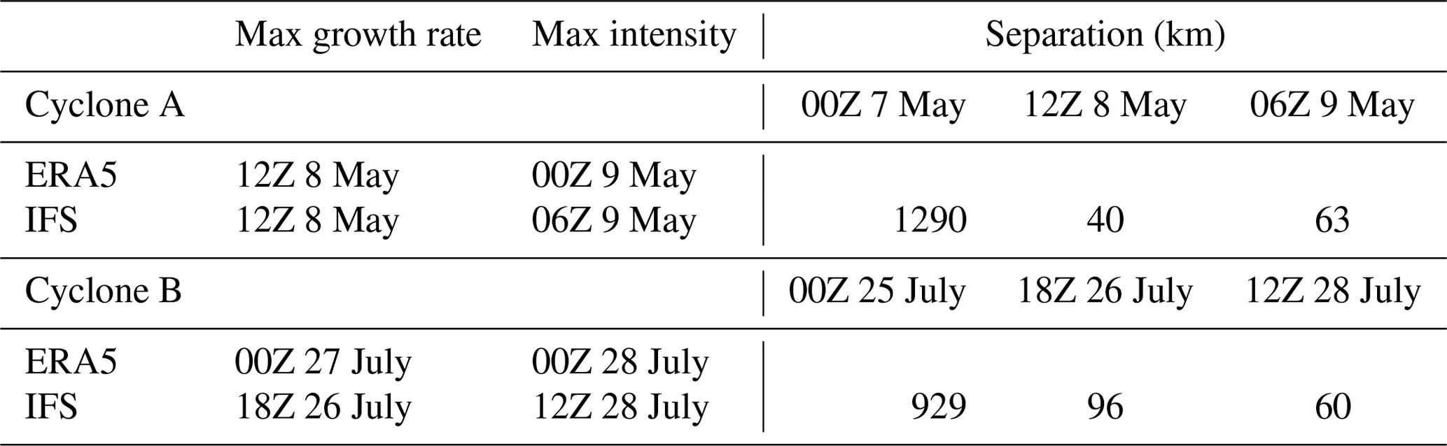
The cyclone case studies were analysed in both the ERA5 reanalysis dataset and IFS forecasts (Table 1). IFS forecast start times (starting at 00Z) were selected that were closest to, but more than 24 h before, the time of maximum growth rate of each cyclone. Consequently, 00Z 7 May and 00Z 25 July are the chosen forecast start dates used for Cyclones A and B respectively throughout the paper. The maximum growth rate of Cyclone A occurred at 12Z 8 May in both ERA5 and the IFS forecasts, with the system reaching maximum intensity 12 h later at 00Z 9 May in ERA5 and 18 h later at 06Z 9 May in the IFS forecast. In ERA5, Cyclone B underwent maximum growth at 00Z 27 July and reached maximum intensity at 00Z 28 July, compared to 18Z 26 July and 12Z 28 July respectively in the IFS forecast.
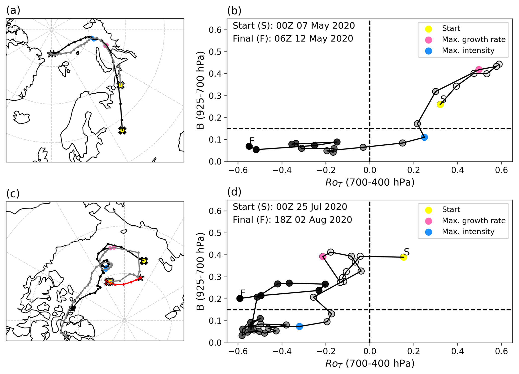
Figure 2(a) The 6-hourly Cyclone A tracks from ERA5 (T5–63; black line) and the IFS run starting 00Z 7 May 2020 (T5–42; grey line) over the shared temporal coverage period 00Z 7 May–06Z 12 May 2020. The start of the tracks is marked by a cross, whilst the end is marked by a star. Note that the full length of the tracks are 18Z 6 May–06Z 12 May (ERA5) and 00Z 7 May–12Z 12 May (IFS). (b) Cyclone A from ERA5 in the adapted cyclone phase-space, from S (start; white) to F (finish; black). The coloured points in (a) and (b) correspond to the times in Table 1: 00Z 7 May (yellow), 12Z 8 May (pink), and 06Z 9 May (blue). (c) As in (a) but for Cyclone B, with IFS run starting 00Z 25 July 2020 over the shared temporal coverage period 00Z 25 July–18Z 2 August 2020. Note that the full length of the tracks are 18Z 24 July–18Z 2 August (primary ERA5; black line), 06Z 14 July–06Z 26 July (secondary ERA5; red line), and 00Z 25 July–12Z 8 August (IFS; grey line). (d) As in (b) but for Cyclone B. The coloured points in (c) and (d) correspond to the times in Table 1: 00Z 25 May (yellow), 18Z 26 July (pink), and 12Z 28 July (blue).
Table 1Summary table of Cyclones A and B tracked using filtered data from ERA5 (T5–63) and the IFS forecasts (T5–42): the time of maximum growth rate, the time of maximum intensity (as evaluated from the tracks), and the great circle separation distance between the cyclone tracks in ERA5 and the IFS forecasts at three selected times (forecast start date, maximum growth rate, and maximum intensity).
Cyclone A developed as part of a baroclinic wave over western Russia before moving northwards into the Kara Sea (Fig. 2a). In both ERA5 and the IFS forecast, the cyclone develops along an elongated low-level front; however, the tracking algorithm identifies the cyclone centres at different places along the feature at 00Z 7 May (likely due to uncertainty in the position of the frontal wave along the front). As the system develops, the tracks converge. This can be seen in Table 1, with the separation reducing from 1290 km at the start of the forecast to 40 km at maximum growth rate, and also spatially in Fig. 2a. The evolution of the cyclone structure is demonstrated by the adapted cyclone phase space (Sect. 2.4) in Fig. 2b. The system is initially low-level dominant (low-level warm core) with large baroclinicity around the time of maximum growth rate. Approaching maximum intensity, and at subsequent times, the cyclone becomes more axisymmetric and ultimately becomes upper-level dominant (cold core).
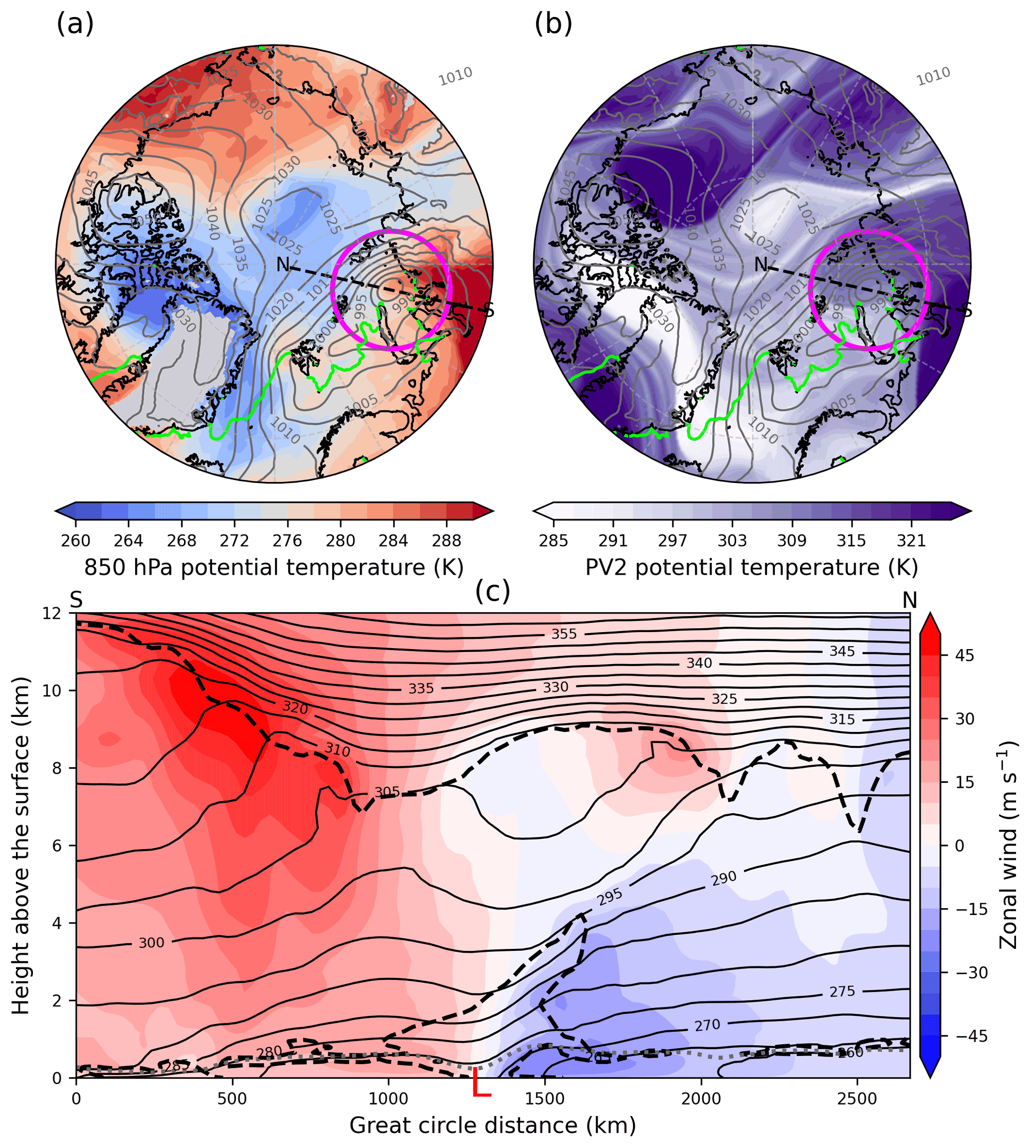
Figure 3Cyclone A at 18Z 8 May 2020 from IFS run starting 00Z 7 May 2020. (a) 850 hPa potential temperature (K; shading) and (b) potential temperature on the PV2 surface (K; shading), overlain with mean sea level pressure (hPa; grey contours) and the sea ice edge (0.15 sea ice concentration; green contour). The magenta circle marks the 750 km radius about the cyclone centre as determined by TRACK. The dashed black lines mark the north–south cross-section taken at the longitude of the cyclone centre from south (65∘ N) to north (89∘ N). (c) Vertical cross-sections linearly interpolated at 100 points between south and north of zonal wind (m s−1; shading), potential temperature (K; solid black contours), 2 PVU contour (dashed black line), and BL top (dotted grey line). Minimum mean sea level pressure is marked with a red L.
Maps of Cyclone A at 6 h after the time of maximum growth rate from the IFS forecast are presented in Fig. 3. The surface cyclone is in the Kara Sea at this time, with the warm sector to the south over Russia (identified by the region of the high values of 850 hPa potential temperature to the south of the cyclone) and the warm front on the eastern flank of the warm sector (Fig. 3a). The cyclone is positioned downstream of an upper-level trough, identified by low potential temperature values on the dynamic tropopause (i.e. the 2 PVU surface; Fig. 3b). A meridional cross-section is taken through the cyclone centre from 65∘ N (S) to 89∘ N (N). In vertical cross-section (Fig. 3c) the tilted isentropes are indicative of a baroclinic zone to the poleward side of the cyclone associated with a developing bent-back front. The upper-level trough is seen as a lowering of the tropopause to the south of the low-level cyclone (7 km height, 305 K), with the downstream ridge situated north of the low centre (9 km height, 310 K). The dip in the isentropes over the cyclone centre (marked by the red L) indicates a warm-core structure developing, consistent with a low-level-dominant cyclone and the strongest winds just above the BL. The positive PV at low levels above the low centre is reminiscent of that generated due to the frictional baroclinic PV mechanism in mid-latitude cyclones (e.g. Adamson et al., 2006).
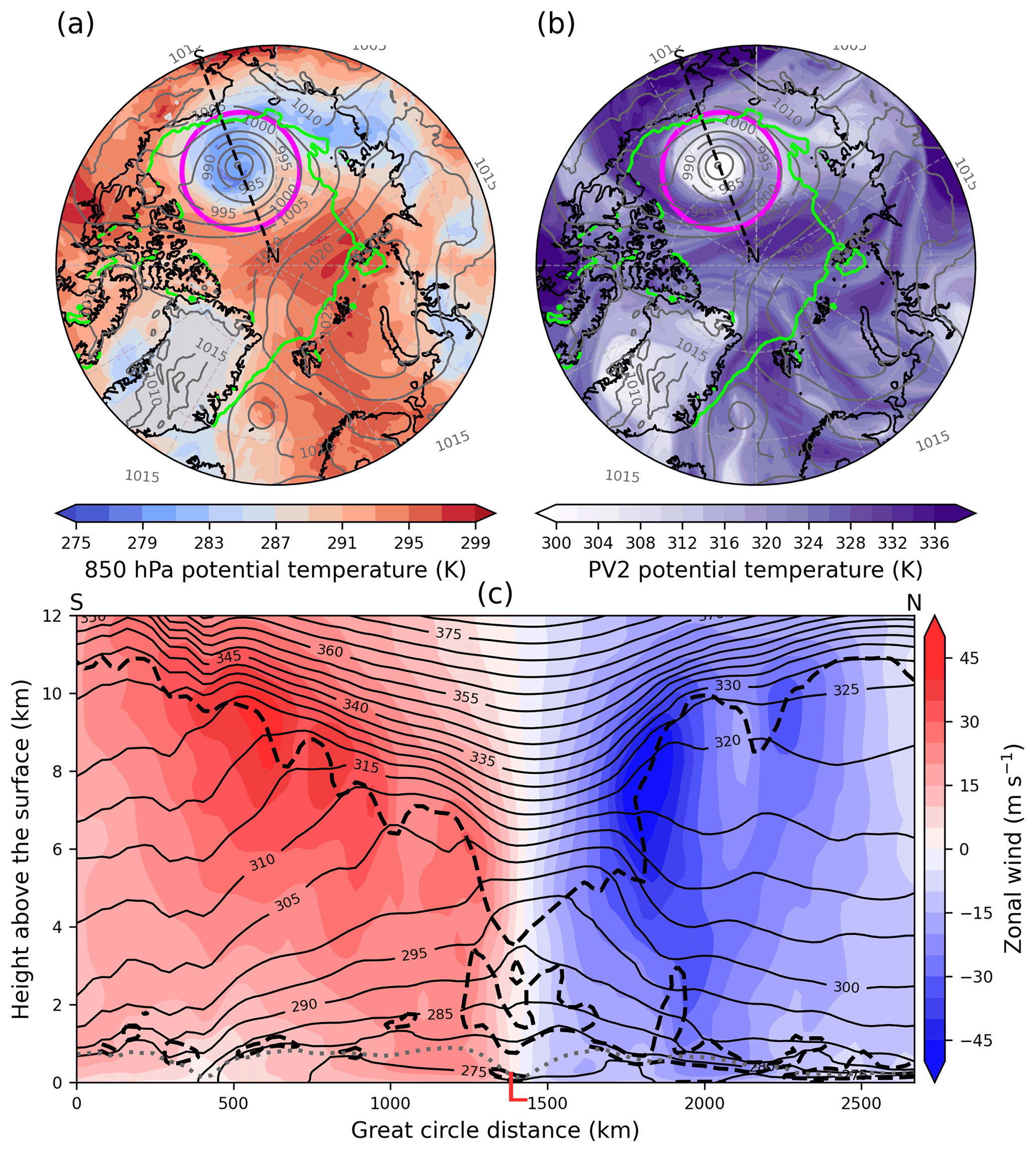
Figure 4As in Fig. 3 but for Cyclone B from IFS run starting 00Z 25 July 2020 at 12Z 28 July 2020.
Cyclone B initially develops baroclinically north of the AFZ along the Eurasian coastline before interacting with a TPV in the Beaufort Sea (Fig. 2c). The cyclone track from ERA5 captures the low-level baroclinic growth phase, with the vorticity maximum north of the Eurasian coastline (black line in Fig. 2c). The TPV in this case is very long-lived and can be tracked back to 8 July 2020 (not shown). There is a secondary track from ERA5, following a low-level vorticity maximum below the pre-existing TPV (red track in Fig. 2c). This track ends once the TPV begins to interact with the low-level baroclinic disturbance at 06Z 26 July. The IFS forecast track (grey track in Fig. 2c) picks up this vorticity maxima associated with the TPV rather than the initial baroclinic disturbance (likely due to the differences between the reanalysis and forecast or the different spectral filtering employed). As a result, the separation between the tracks is initially large but reduces as the cyclone develops (Table 1). From the ERA5 track in the cyclone phase space, Cyclone B is initially baroclinic and low-level dominant (labelled S) but becomes upper-level dominant due to the interaction with the TPV (Fig. 2d). After maximum intensity the cyclone obtains a long-lived (∼4 d) axisymmetric cold-core columnar vortex structure in the Beaufort Sea.
Maps of Cyclone B at maximum intensity from the IFS forecast are presented in Fig. 4. The surface cyclone is located over the sea ice in the Beaufort Sea at this time, associated with a cold air mass at low levels (Fig. 4a), and the TPV is vertically stacked above the cyclone (low potential temperature values in Fig. 4b). In the cross-section the axisymmetric cold-core structure is evident with isentropes bowing up throughout the troposphere centred over the cyclone (Fig. 4c). The TPV is evident as a lowering of the tropopause to ∼4 km. The peak winds of the system are on the flanks of the TPV, consistent with the cold-core and upper-level-dominant system. The cold-core columnar vortex structure of Cyclone B looks quite different to that of a typical mid-latitude cyclone. There is some low-level PV above the BL in the vicinity of the cyclone but not in a coherent region above the cyclone centre as in Cyclone A.
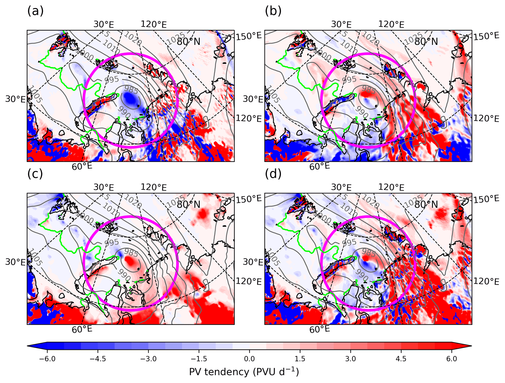
Figure 5BL depth-averaged PV tendencies from Eq. (11) for Cyclone A at 18Z 8 May 2020 (6 h before maximum growth rate) from IFS run starting 00Z 7 May 2020. (a) FEK, (b) FBG, (c) SV, and (d) the sum of FEK, FBG, SV, and SH (PVU d−1; shading), including mean sea level pressure (hPa; grey contours) and the sea ice edge (0.15 sea ice concentration; green contour). The magenta circle marks 750 km from the cyclone centre.
4.1 Boundary layer PV tendencies
The BL PV tendencies from Eq. (11) are presented for Cyclone A at 6 h before maximum growth rate (Fig. 5). The Ekman friction term, FEK, is negative over the cyclone centre (Fig. 5a), indicative of the Ekman pumping mechanism. The frictional baroclinic generation term, FBG, is positive to the north and east of the cyclone centre, along the cyclone bent-back warm front (Fig. 5b), as seen in the typical developing mid-latitude cyclone. The sensible heat flux term, SV, is positive over the cyclone centre and in the warm sector (Fig. 5c), where the atmosphere is warmer than the underlying surface with downward sensible heat fluxes. Note that the SH term is much smaller than the other terms and is therefore not shown in Fig. 5. The sum of the BL PV tendencies (Fig. 5d) resembles the baroclinic generation term, indicating that the Ekman generation is mostly cancelled by the sensible heat flux generation at this time. The BL PV tendencies for Cyclone A resemble those of a typical baroclinic wave mid-latitude cyclone (e.g. Adamson et al., 2006; Boutle et al., 2007).
The BL PV tendencies are presented for Cyclone B at maximum intensity after the cyclone has transitioned to a vertically stacked columnar vortex structure (Fig. 6). As in Cyclone A, the FEK term is negative over the cyclone centre (Fig. 6a), as would be expected in a cyclonic weather system. However, unlike Cyclone A (and typical mid-latitude cyclones), the FBG term is negative, with the largest magnitude to the north and east of the cyclone in the WCB region (Fig. 6b). This is due to the vertically stacked cold-core structure of the cyclone (Figs. 2d and 4), with the cyclonic BL winds oriented in the same direction as the cyclonic winds of the TPV directly aloft (i.e. in the same direction as the tropospheric thermal wind), in contrast to the tilted frontal structure of Cyclone A (see Sect. 5). The SV term is positive, with the largest magnitude in the WCB region (Fig. 6c), indicative of downward sensible heat fluxes over sea ice. This means that the cold air mass associated with the cyclone (Fig. 4a) is still warmer than the sea ice surface, which is locked at 0 ∘C. Like for Cyclone A, the sum of the BL PV tendencies resembles the FBG term, indicating that FEK is mostly cancelled by SV, except for the negative PV tendencies at the cyclone centre where FEK is the dominant term. It is the frictional baroclinic PV generation term, FBG, that distinguishes Cyclone B from Cyclone A (and mid-latitude cyclones).
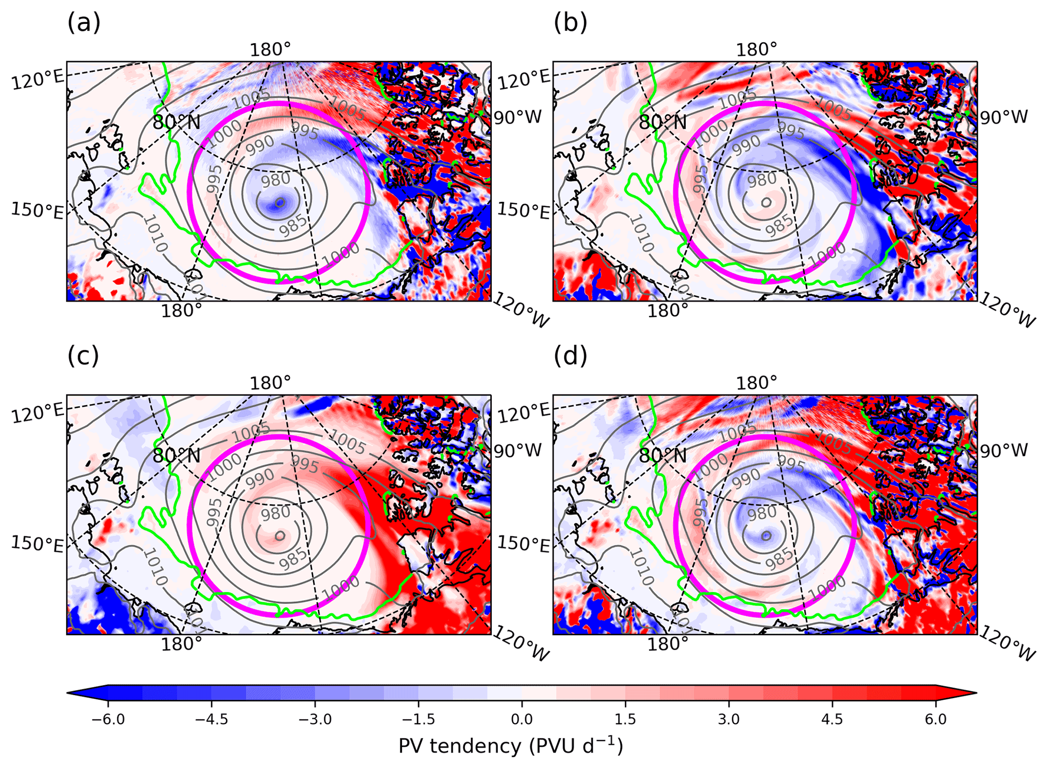
Figure 6As in Fig. 5 but for Cyclone B from IFS run starting 00Z 25 July 2020 at 12Z 28 July 2020 (maximum intensity).
Boutle et al. (2007) demonstrated that in a mid-latitude cyclone initialised without a meridional surface temperature gradient, the (negative) FEK term dominates over (mostly positive) FBG. Cyclone B has some similarities with this experiment, with the sea ice providing a quasi-uniform surface temperature to limit low-level baroclinicity. However, unlike the Boutle et al. (2007) experiment, the vertically stacked cold-core columnar vortex of Cyclone B results in a large region of negative FBG, which is of a similar magnitude to the FEK term.
4.2 Cyclone depth-integrated PV budget
Time series of the terms relevant to the depth-integrated PV budget of Cyclones A and B are presented in Figs. 7 and 8 respectively. The BL PV tendencies in Figs. 7a and 8a have been multiplied by density and BL height to give a BL depth-integrated PV tendency (see first term on RHS of Eq. 13). Note that the y scale in Fig. 7a is almost an order of magnitude larger than in Fig. 8a due to the larger magnitudes of FBG and SV in Cyclone A during development. The larger magnitude of FBG might be due to greater surface roughness over land or greater baroclinicity. The surface energy balance is also changed over land, resulting in large downward sensible heat fluxes and a large SV term.
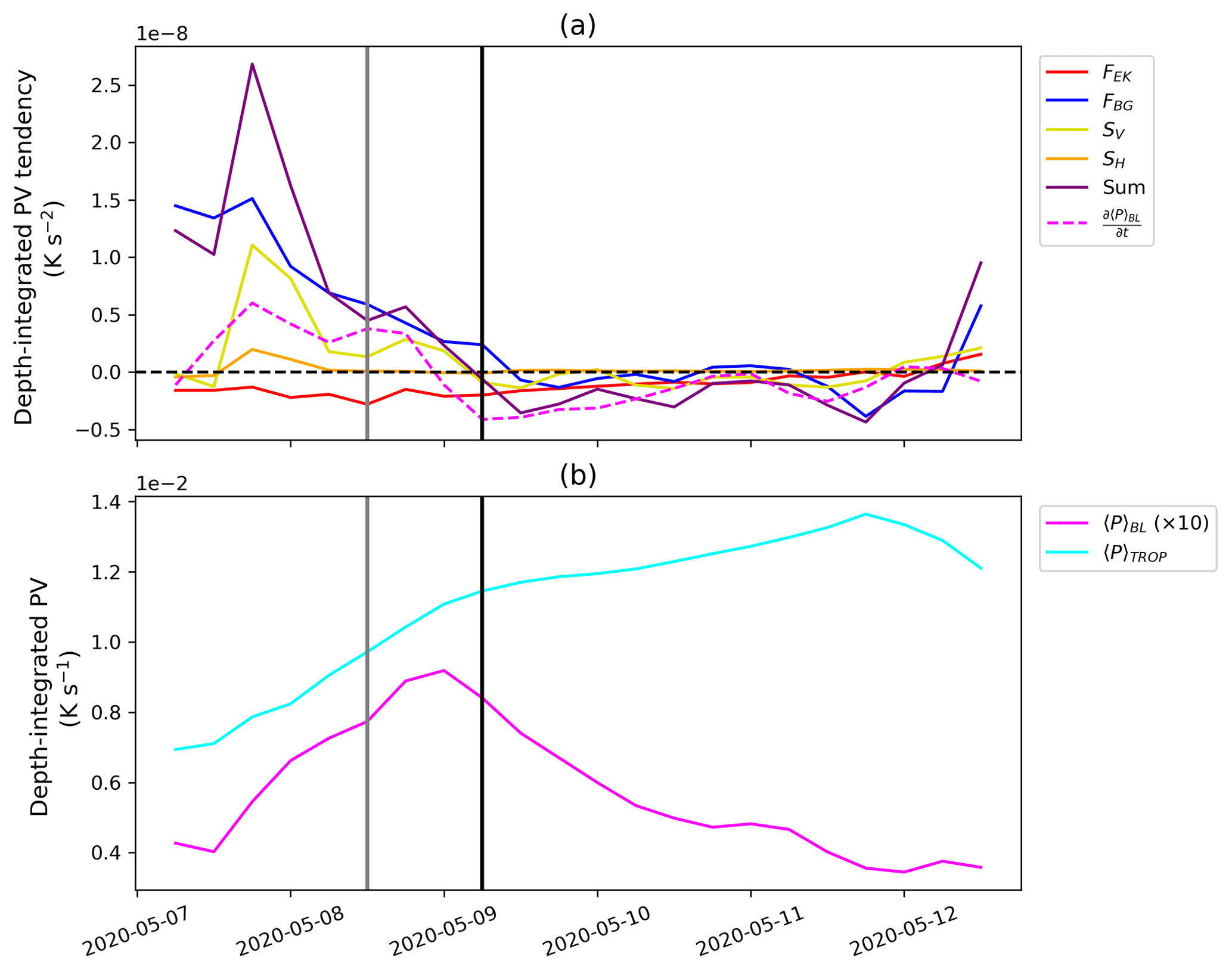
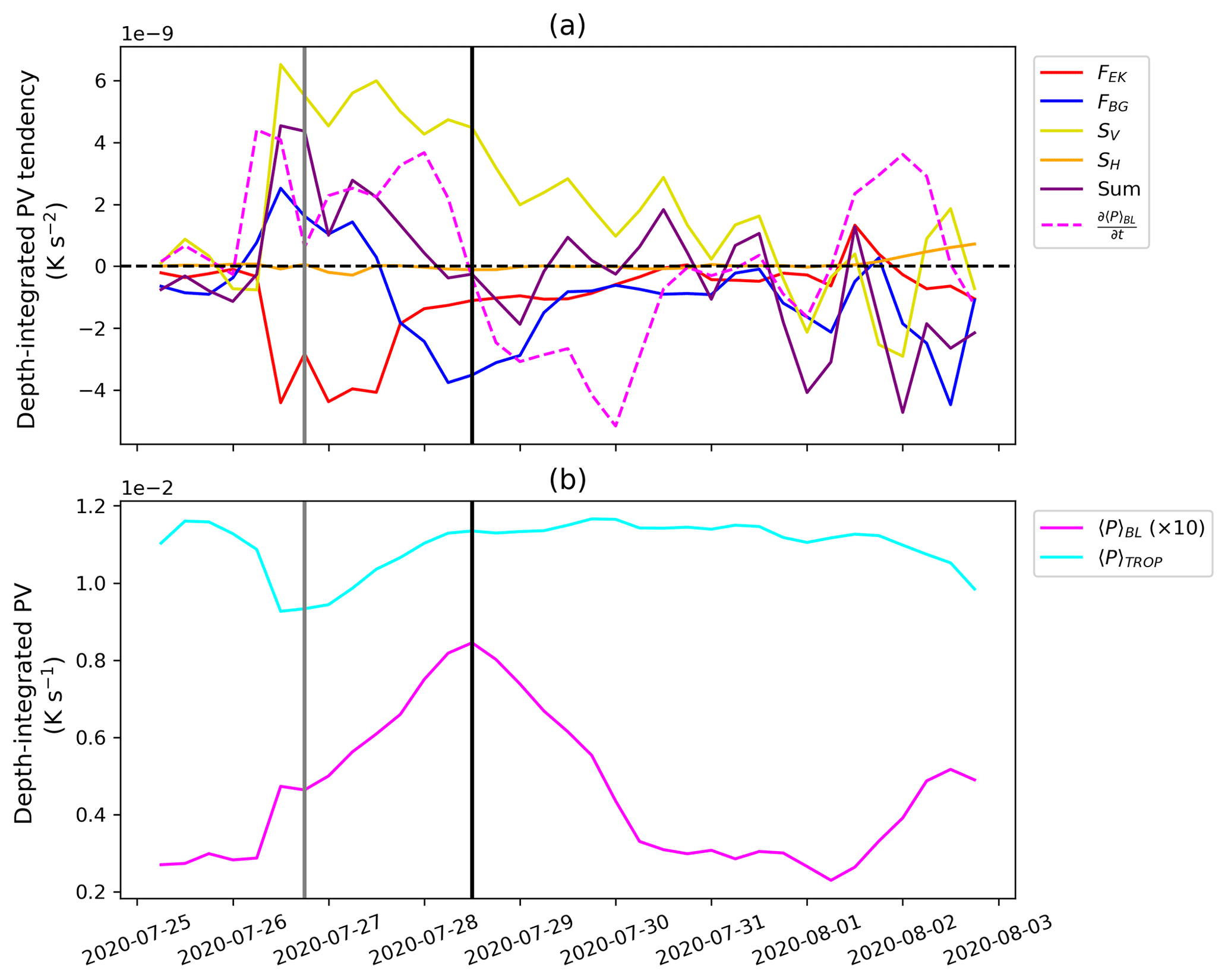
Figure 7Time series of depth-integrated PV and tendencies associated with Cyclone A, from IFS run starting 00Z 7 May 2020, from 00Z 7 May to 12Z 12 May 2020. (a) BL depth-integrated PV tendencies (K s−2): FEK (red line), FBG (blue line), SV (yellow line), SH (orange line), sum (purple line), and the BL volume-averaged PV tendency calculated explicitly (LHS of Eq. 14; dashed magenta line). (b) Volume-averaged PV (K s−1) in the BL and the tropospheric layer with the 330 K isentropic surface as the top of the layer. The grey and black vertical lines correspond to the time of maximum growth rate and maximum intensity.
More generally, the magnitude of the BL PV tendencies is impacted by several (interrelated) factors, including the underlying surface, cyclone strength, and BL height, h. For instance, stronger cyclone winds correspond with larger vorticity and surface fluxes and therefore larger PV tendencies Eq. (11). Furthermore, the depth-integrated PV tendencies scale by such that the magnitude decreases with increasing h. Cyclone A has stronger low-level winds than upper-level-dominant Cyclone B but with stable shear-driven BLs also has a slightly higher h (with an average value of ∼800 m at maximum intensity compared to ∼600 m), with opposing effects on the magnitude of the BL PV tendencies. Clearly, the magnitude of the BL PV tendencies varies with cyclone-specific details, which differ between any two cyclones. However, in this study, we are focused on the fundamental mechanisms in cyclones with contrasting structure, so it is the general evolution and sign of the BL PV tendencies that are the main interest rather than the absolute magnitude. In the subsequent analysis, we focus on the general evolution and sign when comparing the case studies.
In Cyclone A (Fig. 7a), the Ekman friction (FEK) term is negative throughout the time series, indicative of the Ekman pumping mechanism acting throughout the cyclone evolution. The baroclinic PV generation (FBG) term is large and positive during the baroclinic growth phase before the maximum intensity, with a reduced magnitude after this time (and becoming generally negative). The sensible heat flux (SV) term is positive before the time of maximum intensity, dominated by the strong downward heat fluxes in the warm sector (Fig. 5c). After maximum intensity the SV term has a smaller magnitude. The SH term (proportional to the horizontal gradient of sensible heat fluxes) is also presented in Fig. 7a and has a much smaller magnitude than the other non-conservative terms. The sum of the BL PV tendencies is positive during the baroclinic growth phase (before maximum intensity), dominated by FBG, and is negative once the cyclone has matured.
The volume-averaged PV in the BL, 〈P〉BL (Sect. 2.6), of Cyclone A (Fig. 7b) increases during the baroclinic growth phase up to 6 h before maximum intensity and decreases after. The rate of change of 〈P〉BL is plotted against the BL PV tendency terms in Fig. 7a (dashed pink line) and corresponds well with the sum of the non-conservative terms (purple line). However, the sum of the non-conservative terms has a larger magnitude before maximum growth rate, which indicates that the vertical and horizontal fluxes of PV into or out of the BL control volume are large at this time, according to Eq. (13). The volume-averaged PV in the tropospheric layer, 〈P〉TROP, increases throughout the cyclone lifetime, even after the time of maximum intensity of the low-level cyclone. The increase in 〈P〉TROP is dominated by baroclinic wave growth, which in this budget is apparent through the lateral PV fluxes into the volume. Note that 〈P〉TROP is approximately 15 times larger than 〈P〉BL. The fractional rate of growth in the BL and tropospheric layer is similar up to maximum growth rate (i.e. the slopes of 〈P〉BL and 〈P〉TROP are similar), which is characteristic of system growth with the BL and upper levels coupled (i.e. lateral PV fluxes in Eqs. 13 and 14 are linked due to the baroclinic tilt of system that is continuous across both layers). Hence, the same BL processes that impact the BL circulation will have an indirect effect on the tropospheric layer also.
In Cyclone B (Fig. 8) the Ekman friction (FEK) term is negative with maximum magnitude during the baroclinic growth phase at maximum growth rate (Fig. 8a). The baroclinic PV generation (FBG) term captures two distinct periods of cyclone development. FBG is positive during the baroclinic growth phase but is approximately an order of magnitude smaller than in Cyclone A (Fig. 7a), indicating reduced baroclinicity. After the time of maximum growth rate, FBG reduces and rapidly becomes strongly negative, decreasing to an absolute minimum 6 h before maximum intensity. The evolution of FBG differs from that of Cyclone A, with the transition from positive to negative occurring before maximum intensity for Cyclone B and the negative FBG values having a larger magnitude (relative to the magnitude of the positive values before transition). The sensible heat flux (SV) term is largely positive due to downward sensible heat fluxes over the sea ice. The sum of the non-conservative BL terms is positive before maximum intensity, dominated by the SV term, and is close to zero afterwards with the positive SV term reducing in magnitude and having a greater (negative) contribution from FBG. Note that the magnitude of FBG is greater than FEK in Cyclone A (a more baroclinic cyclone; Fig. 7a), whereas their magnitudes are comparable in Cyclone B due to a more barotropic structure (Fig. 8a).
Volume-averaged PV in the BL, 〈P〉BL, of Cyclone B increases during the baroclinic growth phase up to maximum intensity and decreases after (Fig. 8b), similar to that in Cyclone A in profile and magnitude (Fig. 7b). The rate of change of 〈P〉BL (Fig. 8a) corresponds well with the sum of the BL non-conservative terms. The differences between the two series is likely due to vertical and horizontal PV flux terms and also possibly latent heating (which is not explicitly calculated here). Unlike in Cyclone A, 〈P〉TROP is relatively constant (Fig. 8b). This is related to the pre-existing TPV associated with Cyclone B. Applying a similar reasoning used in Martínez-Alvarado et al. (2016), if the control volume containing the TPV is in an isentropic layer (i.e. the BL top is an isentropic surface as well as the top boundary), and all the non-conservative processes lie within the circuit, then the circulation is conserved if the lateral boundary is a material surface. When the system (TPV and low-level cyclone) becomes a cut-off axisymmetric circuit, this condition is satisfied, and the circulation (〈P〉) is conserved. Cyclone B largely satisfies this condition, except during the baroclinic growth phase (i.e. the dip in 〈P〉TROP in Fig. 8b at maximum growth rate), when the cyclone and TPV start to interact. The coupling between the BL and tropospheric layer is reduced such that the BL processes do not significantly impact the free-tropospheric circulation at this stage. This is very different to the evolution of the system 〈P〉 in Cyclone A (Fig. 7).
This analysis has revealed how the magnitude and sign of the cyclone-average BL PV tendencies evolve in time and how the baroclinic PV generation term, FBG, differs between the cyclones. A key question is the extent to which this difference modifies the subsequent evolution of the cyclones. Whilst a quantitative assessment of this effect, which would require a piecewise PV inversion procedure, is beyond the scope of this work, in the following section the impacts of the BL processes are qualitatively inferred by analysing the 3-D structure of the cyclones and their associated PV fields. In Sect. 5 the FBG term is examined in more detail.
4.3 Cyclone structural evolution
Low-level (up to 700 hPa) north–south cross-sections of Cyclone A at selected times are presented in Fig. 9. The panel below each cross-section shows the profile of the (depth-averaged) BL PV tendency terms interpolated along the section (just shown within 750 km of the cyclone centre for clarity). At the time of maximum growth rate (Fig. 9a) the cyclone has a baroclinic tilted structure, with tilted isentropes associated with positive PV over the cyclone centre. Winds exceed 15 m s−1 in the BL at this time. FEK is negative below the cyclone centre, whilst FBG is positive to the north (where the BL winds are strongest). SV is positive to the south of the cyclone centre, where there are downward sensible heat fluxes in the warm sector. This is consistent with a region of positive PV in the BL on the southern end of the cross-section. The sum of the BL PV tendencies is positive to the north of the cyclone and negative to the south.
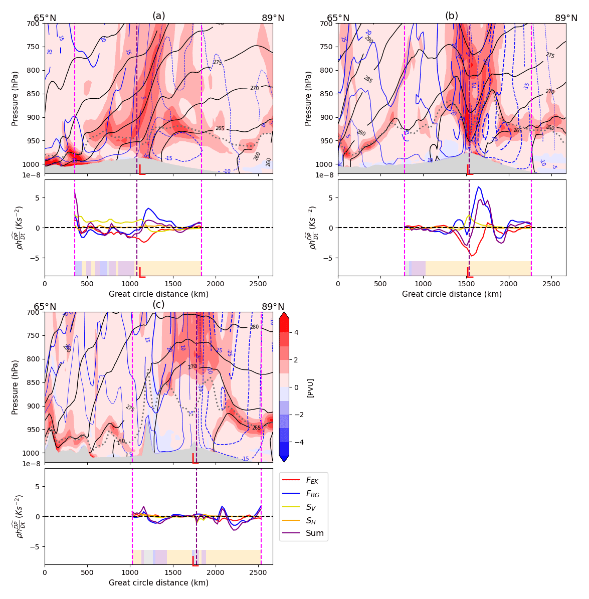
Figure 9North–south cross-sections of Cyclone A, from IFS run starting 00Z 7 May 2020, at the longitude of the cyclone centre from 65 to 89∘ N at (a) 12Z 8 May (maximum growth rate), (b) 06Z 9 May (maximum intensity), and (c) 06Z 10 May 2020 (24 h after maximum intensity). The top panels display potential vorticity (PVU; shading), potential temperature (K; solid black contours), zonal wind (m s−1; blue contours), and the BL top (dotted grey line). The bottom panels display the BL PV tendency terms (scaled to depth-integrated PV tendencies) due to friction and sensible heat fluxes, within 750 km radius of the cyclone centre. The background shading denotes the surface type: land (grey), ocean (blue; sea ice concentration < 0.15), marginal ice zone (purple; sea ice concentration > 0.15 and <0.8), and pack ice (orange; sea ice concentration > 0.8). The purple vertical line marks the cyclone centre from TRACK (Sect. 2.3), and the magenta lines mark 750 km distance from the cyclone centre. Minimum sea level pressure along the section is marked with a red L.
At the time of maximum intensity (Fig. 9b), the system has obtained a warm-core axisymmetric structure over the sea ice, with isentropes dipping down over the low-pressure centre. The system is very strong at low levels this time, with winds speeds exceeding 30 m s−1 in the BL. There is large positive PV above the BL constrained within a ∼200 km radius of the cyclone centre, associated with enhanced static stability, and is likely indicative of the frictional baroclinic PV mechanism. As at maximum growth rate, FEK is negative over the cyclone centre, whilst FBG is positive to the north of the cyclone below the strongest BL winds. The magnitude of SV is reduced at this time. The BL height peaks where the winds are strongest, indicative of a wind-driven BL and consistent with small sensible heat fluxes. The sum of the BL PV tendencies is again positive to the north of the cyclone, consistent with positive PV there, and negative to the south of the cyclone, where there is negative PV.
At 24 h after the time of maximum intensity (Fig. 9c), the cyclone has lost its warm core and has now developed a larger-scale cold-core structure, with the isentropes bowing upwards. This resembles the composite cold-core axisymmetric structure of summer-time Arctic cyclones after maximum intensity from Vessey et al. (2022). The isentropes have moved upward, taking the low-level positive PV from 950 hPa up to 800 hPa. The wind field is now upper-level dominant but with a deep structure such that winds still exceed 20 m s−1 in the BL. The BL PV tendencies are now reduced in magnitude (due to weaker winds), but the FBG term is notably the dominant term and is predominantly negative. The negative FBG term is also seen in Fig. 7 after maximum intensity and likely reflects the cyclone's transition to an axisymmetric cold-core structure. The cyclone retains this cold-core axisymmetric structure for 2 more days before dissipating (Fig. 2b).
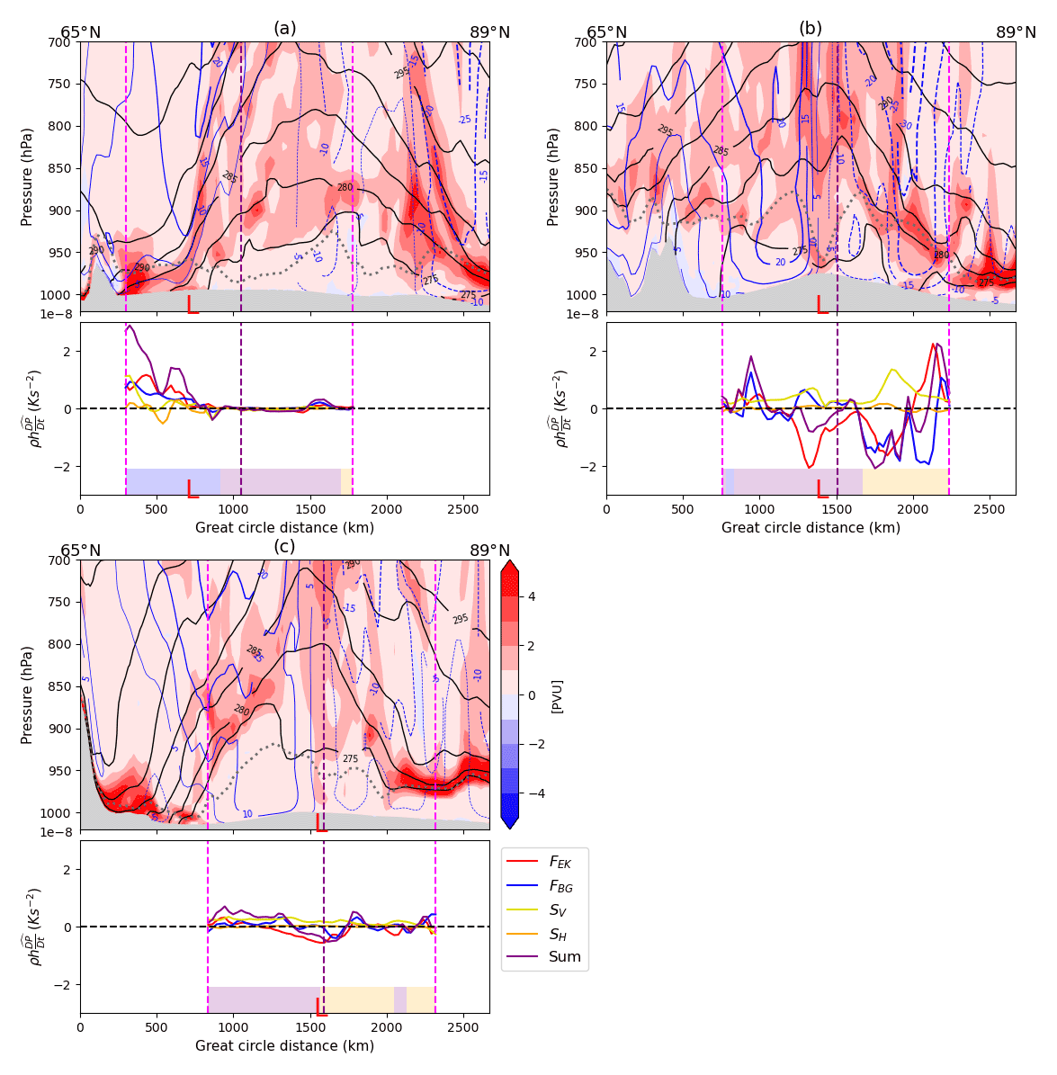
Figure 10As in Fig. 9 but for Cyclone B, from IFS run starting 00Z 25 July 2020, at (a) 18Z 26 July (maximum growth rate), (b) 12Z 28 July (maximum intensity), and (c) 12Z 31 July (72 h after maximum intensity).
This cross-section analysis is also performed for Cyclone B (Fig. 10). At the time of maximum growth rate (Fig. 10a), the cold-core structure of the pre-existing TPV is evident in the isentropes. There are baroclinic zones to the north and south of the TPV, with tilted isentropes and positive near-surface PV. Cyclone B develops on the baroclinic zone to the south of the TPV. The TPV is associated with a strong cyclonic wind field at the tropopause, but this does not extend to the BL at this time. The BL PV tendency terms are largest to the south of the section over the ocean. FEK is positive, which is consistent with the cyclone centre (as diagnosed by ξ850) not being co-located with the minimum in sea level pressure at this time (not shown). FBG is positive, consistent with the system undergoing baroclinic growth. With SV also being positive, there is net positive PV being generated over the cyclone centre.
At the time of maximum intensity (Fig. 10b), the cyclone has obtained an axisymmetric cold-core structure. The cyclonic winds about the system now extend to the lower levels, with winds greater than 20 m s−1 in the BL. PV is small within the BL at this time. The magnitude of the BL PV tendency terms in Cyclone B is approximately half that of Cyclone A, likely due to the system being upper-level dominant with weaker winds at the surface. FEK is negative over the cyclone centre, and FBG is negative on the northern flank of the cyclone. SV is small but consistently positive over the cyclone.
At 72 h after the time of maximum intensity (Fig. 10c), whilst the surface cyclone has weakened (with BL winds of ∼10 m s−1), the axisymmetric cold-core structure has amplified, with a steeper isentropic tilt on the flanks of the system. The BL PV tendencies are small at this time, although FEK is notably negative over the cyclone centre, indicative of Ekman pumping. Note that the system is not associated with a coherent accumulation of PV above the BL like in Cyclone A, and consequently there is reduced static stability above the BL here (i.e. the isentropic surfaces are spaced further apart).
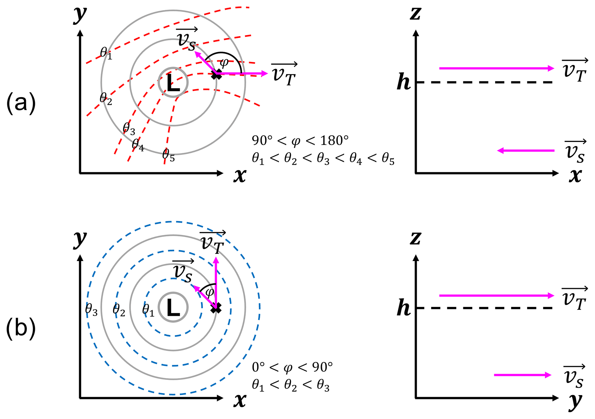
Figure 11Schematics of (a) low-level-dominant (warm-core) and (b) upper-level-dominant (cold-core) cyclone structures. Left panels show plan views of cyclone with mean sea level pressure (solid grey contours) and potential temperature (θ; dashed contours). At the point marked by the black cross, the orientation of the surface wind vector (vS; in the same direction as the surface stress, τS) and the thermal wind vector above the BL (vT) are demonstrated by the magenta arrows, with an angle ϕ between them. Right panels show vertical wind structure at this point, with the horizontal axis aligned with the largest component of vT: in (a) this is the x direction, and in (b) this is the y direction. The orientation of vS and vT are demonstrated with magenta arrows. The BL top is marked by the dashed black line (height h). The idealised cyclone structure in (a) is associated with positive FBG, whilst (b) is associated with negative FBG.
From the results, the BL process that most obviously differs between Cyclones A and B is frictional baroclinic PV generation, i.e. the FBG term. Physically, the FBG term is governed by the orientation of the surface winds and the low-level thermal wind above the BL. Another form of thermal wind balance is
where is the thermal wind vector, vT, just above the BL. Substituting Eq. (15) into the FBG term in Eq. (11) gives FBG explicitly in terms of the thermal wind just above the BL:
where ϕ is the angle between τS and vT, and τS is in the same direction as the surface wind (vS). Schematics of low-level-dominant and upper-level-dominant cyclones are presented in Fig. 11. In the low-level-dominant case (Fig. 11a), in the warm-front region, the cyclonic BL wind opposes the low-level thermal wind vector just above the BL. Hence, τS and vT are opposed (i.e. ). According to Eq. (16), this would yield a positive Lagrangian PV tendency (FBG), consistent with that in Cyclone A. Now consider an axisymmetric upper-level-dominant cyclone (Fig. 11b). The cyclonic BL wind is oriented in the same direction as the low-level thermal wind vector just above the BL. This means that τS and vT are oriented in the same direction (i.e. ) such that the Lagrangian PV tendency (FBG) in Eq. (16) is negative. This is consistent with the sign of FBG associated with Cyclone B.
In essence, FBG represents changes in PV due to BL friction altering the horizontal components of vorticity. FBG can be written as the Lagrangian derivative of the horizontal component (considering only the y component for simplicity) of Eq. (1):
where the product rule has been applied to give the RHS, and variations in density have been neglected. The horizontal vorticity in the BL, , is associated with the (zonal) vertical wind shear between the surface winds and the thermal wind just above the BL. Therefore FBG depends on the vertical wind shear across the BL () and the horizontal temperature gradient just above the BL top ().
Once again, consider the warm-front region of a low-level-dominant cyclone, where the cyclonic BL wind opposes the low-level thermal wind vector (Fig. 11a). In this setup, , and . Friction will act to slow down the BL winds such that the vertical wind shear over the BL is reduced: . If the system is to remain in thermal wind balance, the temperature gradient (just above the BL) across the cyclone must also weaken: (note that this yields FBG>0 from Eq. 17). The reduction in the temperature gradient across the cyclone means that the cyclone warm core decays.
Now consider an axisymmetric upper-level-dominant or cold-core cyclone (Fig. 11b), where the cyclonic BL wind is oriented in the same direction as the low-level (cyclonic) thermal wind vector above the BL. Here, , and . Friction slows down the BL winds, which in this configuration will increase the vertical wind shear over the BL: . To remain in thermal wind balance, the temperature gradient (just above the BL) across the cyclone must increase: (note that this yields FBG<0 from Eq. 17). The increase in the temperature gradient across the cyclone means that the cyclone cold core intensifies.
It has been shown that FBG has the opposite impact on cyclone thermal structure. In low-level-dominant cyclones, the thermal anomaly is weakened, whereas in upper-level-dominant cyclones, the thermal anomaly is amplified. The analysis demonstrates that the impact of friction depends on the cyclone structure. In both cases, FBG is acting to cool the thermal anomaly.
For Cyclone A, the analysis above demonstrates that FBG acts to decay the low-level warm core (and amplify the cold-core anomaly once established; see negative FBG after maximum intensity in Fig. 7). Ekman pumping is also acting, which will also cool the system due to the rising of air and adiabatic cooling (Ekman pumping is also acting to spin down the cyclone as it becomes stacked in the vertical). The positive SV term (before maximum intensity; Fig. 7), indicative of downward sensible heat fluxes, also contributes to cooling with the atmosphere losing heat to the surface. For Cyclone B, FBG acts to amplify the cold core, with Ekman pumping and sustained downward sensible heat fluxes over the sea ice (as indicated by negative FEK and positive SV; Fig. 8) also contributing to low-level cooling. Hence, all of the BL PV tendencies in both cyclones are contributing to cooling the system. Low-level cooling in an axisymmetric cyclone will result in a reduction in low-level vorticity and therefore a reduction in surface winds. This can be shown using Eq. (3); for example, in a cold-core cyclone will increase in magnitude, and therefore will increase. Assuming upper-level vorticity and the layer depth stays constant, this means the low-level vorticity must decrease. Hence, the frictional processes and sensible heat fluxes are contributing to weakening the low-level cyclone after maximum intensity. Although the low-level cyclone is weakening, friction is acting to amplify a cold-core anomaly above the BL in both cyclones once they have matured. What this means for the subsequent system evolution is still an open question.
Consistent with all of the BL processes contributing to cooling the system, both cyclones obtain a vertically stacked cold-core structure after maximum intensity (Figs. 9c and 10c) which persists for several days (Fig. 2b and d). This structural evolution is not seen in maturing mid-latitude cyclones. The barotropic cold-core structure after maximum intensity resembles the structural transition of summer-time Arctic cyclones in Vessey et al. (2022). Vessey et al. (2022) find that their summer-time Arctic cyclone composite does not undergo occlusion and suggest that summer-time Arctic cyclones may lack the dynamical forcing from the occlusion process that typically leads to the dissipation of mid-latitude cyclones. One hypothesis is that this may extend the lifetime of summer-time Arctic cyclones. This will allow BL processes (which all act to cool the thermal anomaly in Cyclones A and B) to act over a longer time period than in mid-latitude cyclones, permitting the cold-core structure to develop and persist over many days.
In Cyclone A, Ekman pumping and the baroclinic PV mechanism are both acting to increase the static stability above the BL (Boutle et al., 2015). This acts to reduce the coupling of the lower and upper levels and eventually weaken the cyclone. In Cyclone B, the static stability above the BL is reduced compared to Cyclone A (see the large vertical spacing of the isentropes above the BL in Fig. 10c). The lower static stability would result in enhanced coupling of the lower and upper levels for longer (compared to Cyclone A) and might explain the longer lifetime of Cyclone B (almost 10 d) compared to Cyclone A (∼6 d).
Previous studies have demonstrated that the evolution of mid-latitude cyclones is sensitive to BL turbulent fluxes (e.g. Valdes and Hoskins, 1988) and identified the BL processes by which the surface influences mid-latitude cyclones (e.g. Cooper et al., 1992; Adamson et al., 2006). However, the influence of the surface and the relevant dynamical mechanisms have not yet been investigated in the context of Arctic cyclones. Differences are expected for several reasons. Firstly, surface properties (and therefore turbulent fluxes) are highly variable in the summer-time Arctic over land, ocean, marginal ice, and pack ice. Secondly, Arctic cyclones are longer lived than mid-latitude cyclones, allowing BL processes to act for longer. Thirdly, there are different cyclone growth mechanisms and morphologies in the Arctic such that the BL processes may have different impacts on cyclone evolution.
The purpose of this study is to characterise the BL processes acting in summer-time Arctic cyclones and understand how they influence the structural evolution. A PV framework (derived by Cooper et al., 1992, in the Vannière et al., 2016, form) has been used, as has been used in previous studies for mid-latitude cyclones (e.g. Adamson et al., 2006; Plant and Belcher, 2007). This PV framework in Eq. (11) reveals four BL PV tendencies, each representing a BL process, associated with friction or sensible heat fluxes: FEK (Ekman friction), FBG (frictional baroclinic PV generation), SV (sensible heat fluxes), and SH (proportional to the horizontal gradient of sensible heat fluxes – typically smaller than the other terms). In this work, unlike previous studies, summer-time Arctic cyclones are categorised by their vorticity structure during development as either (i) low-level dominant (low-level warm core) or (ii) upper-level dominant (tropospheric cold core). In this study, BL processes (and their impact on cyclone evolution) acting in two contrasting cyclone case studies from summer 2020 are investigated and compared. Cyclone A occurred in May 2020 and was low-level dominant (developing as part of a baroclinic wave off the Eurasian coastline), whilst Cyclone B occurred in July 2020 and was upper-level dominant (developing with a TPV in the Beaufort Sea). The primary tool used is the ECMWF global IFS model, focusing on a single model run for each cyclone.
The first research question (defined in Sect. 1) was to determine the nature of the BL processes in the different types of Arctic cyclones, and the second was to understand how these evolve with time. Both Cyclones A and B are associated with negative FEK, and therefore Ekman pumping, which acts to spin down the cyclones throughout their lifetime (as would be expected in cyclonic weather systems). Furthermore, both cyclones are associated with positive SV due to downward sensible heat fluxes over sea ice (i.e. the atmosphere losing heat to the underlying surface), representing the generation of PV due to increased static stability. Cyclone A is associated with positive SV before maximum intensity in the warm sector (over land and sea ice). Cyclone B is associated with positive SV over the sea ice for most of its lifetime. It is the frictional baroclinic PV generation, the FBG term, that differs between Cyclones A and B. The FBG term is positive in Cyclone A along the warm-front region during the baroclinic growth phase, where the BL winds oppose the lower-tropospheric thermal wind. After maximum intensity this term reduces in magnitude and becomes weakly negative. In Cyclone B, FBG is initially positive during the baroclinic growth phase (but with a reduced magnitude compared to Cyclone A, suggesting reduced baroclinicity). As the system approaches maximum intensity, the FBG term becomes strongly negative, as the cyclone becomes vertically stacked, with BL winds in the cyclone oriented in the same direction as the cyclonic thermal wind associated with the TPV above the BL. In both cyclones the sum of the BL PV tendencies are positive before maximum intensity and negative afterwards.
Comparisons of the BL processes acting in Cyclones A and B with those in mid-latitude cyclones were made throughout the article. The evolution of Cyclone A resembles that of mid-latitude cyclones, consistent with the same frictional processes, with negative FEK and positive FBG. There is also evidence of the baroclinic PV mechanism, the dominant frictional spin-down mechanism in baroclinic wave cyclones, with a region of high PV just above the BL over the low centre in Cyclone A (e.g. Adamson et al., 2006). In contrast, Cyclone B is associated with negative FBG due to the vertically stacked nature of the system with a TPV, suggesting that friction is acting differently compared to Cyclone A and typical mid-latitude cyclones. Both cyclones are associated with predominantly positive SV due to downward sensible heat fluxes over the sea ice, unlike mid-latitude cyclones. The SV term is generally small in Cyclone A (except over land), consistent with the finding from Haualand and Spengler (2020) that sensible heat fluxes only have a minor impact on baroclinic wave development. In contrast, the SV term is more dominant in Cyclone B, with downward sensible heat fluxes over sea ice over the entire cyclone.
Finally, the third research question was to understand the impact of the BL processes on the Arctic cyclone interior evolution. It has been shown that the FBG term has the opposite impact on cyclone structure above the BL, depending on the cyclone type. In Cyclone A (low-level dominant), FBG acts to decay the warm-core thermal anomaly, whereas FBG acts to amplify the cold-core thermal anomaly in Cyclone B (upper-level dominant). In fact, all of the BL processes associated with friction and sensible heat fluxes are contributing to lower-tropospheric cooling and therefore a reduction in low-level vorticity by thermal wind balance. Although the low-level circulation of the cyclone is weakening, friction is acting to amplify a cold-core anomaly above the BL. Consistent with the BL processes contributing to cooling, both Cyclones A and B obtain a cold-core structure which persists for several days after maximum intensity, unlike the evolution of mid-latitude cyclones. Vessey et al. (2022) have suggested that Arctic cyclones may lack the dynamical forcing to dissipate as quickly as mid-latitude cyclones, and it is hypothesised that this may allow the BL processes to act over a longer period of time. This may permit the cold-core structure to develop and persist over several days. Finally, it is hypothesised that in Cyclone B, because frictional baroclinic PV generation does not result in high PV (and high static stability) over the cyclone centre, the coupling of the lower and upper levels is prolonged and therefore so is cyclone lifetime (∼10 d) compared to Cyclone A (∼6 d).
Moist processes and diabatic effects in the free troposphere (in particular latent heat release coupled with the vertical motion) have not been considered here. Although we may expect latent heating to be less important in the Arctic than in lower latitudes due to reduced absolute humidity, Terpstra et al. (2015) demonstrated that low-level disturbances are able to amplify in a high-latitude moist baroclinic environment in the absence of other processes (upper-level perturbations, surface fluxes, or radiation) using an idealised baroclinic channel model. This suggests that latent heating can be significant for the development of polar cyclones. The work here is focused on characterising the effects of friction and sensible heat fluxes at the lower boundary on Arctic cyclones in two cases with contrasting structures. The authors are conducting further study to quantify the response of the 3-D wind field within the cyclones to the BL processes explored here, and the amplification of ascent by latent heat release, using the diagnostic tool of Cullen (2018) assuming semi-geostrophic balance dynamics. Quantifying the relative importance of non-conservative processes in the BL and free troposphere in the evolution of Arctic cyclones and understanding the sensitivity of cyclone evolution to surface properties are also areas for future research.
ECMWF IFS forecast data were produced by running ECMWF's IFS model (model cycle 47r1, which was operational from 30 June 2020 to 10 May 2021). These data are stored on ECMWF's Meteorological Archive Retrieval System (MARS) Catalogue, under experiment IDs “b2k2” and `b2mo”. These data are not publicly available but can be provided on request. ECMWF ERA5 reanalysis data were also retrieved via MARS. The ERA5 reanalysis data are publicly available and can be downloaded from the Copernicus Climate Change Service (C3S) Climate Data Store (Hersbach et al., 2017). The TRACK algorithm (Hodges, 1994, 1995) is available on the University of Reading's Git repository (GitLab) at https://gitlab.act.reading.ac.uk/track/track (Hodges, 2021).
HLC designed the study and conducted the analysis detailed in this paper, with supervision from JM, BH, SPEK, and AV. SPEK set up the ECMWF IFS model configurations which were run by HLC. HLC took responsibility to write this paper, with feedback from JM, BH, SPEK, and AV.
The contact author has declared that none of the authors has any competing interests.
Publisher's note: Copernicus Publications remains neutral with regard to jurisdictional claims in published maps and institutional affiliations.
Hannah L. Croad acknowledges funding and support from the SCENARIO NERC Doctoral Training Partnership, with co-supervision and super-computing support from ECMWF. The authors thank Kevin Hodges for providing cyclone tracks from the TRACK algorithm for use in this study. The authors would also like to acknowledge ECMWF for the production of the ERA5 reanalysis dataset.
This research has been supported by PhD studentship funding from SCENARIO NERC Doctoral Training Partnership grant NE/S007261/1 and the Arctic Summer-time Cyclones: Dynamics and Sea-ice Interaction NERC standard grant NE/T006773/1.
This paper was edited by Yang Zhang and reviewed by three anonymous referees.
Adamson, D., Belcher, S. E., Hoskins, B. J., and Plant, R. S.: Boundary-layer friction in midlatitude cyclones, Q. J. Roy. Meteorol. Soc., 132, 101–124, 2006. a, b, c, d, e, f, g, h, i
Aizawa, T. and Tanaka, H.: Axisymmetric structure of the long lasting summer Arctic cyclones, Polar Sci., 10, 192–198, 2016. a
Asplin, M. G., Galley, R., Barber, D. G., and Prinsenberg, S.: Fracture of summer perennial sea ice by ocean swell as a result of Arctic storms, J. Geophys. Res., 117, C06025, 2012. a
Boutle, I., Beare, R., Belcher, S., and Plant, R.: A note on boundary-layer friction in baroclinic cyclones, Q. J. Roy. Meteorol. Soc., 133, 2137–2141, 2007. a, b, c, d, e
Boutle, I. A., Belcher, S. E., and Plant, R. S.: Friction in mid-latitude cyclones: an Ekman-PV mechanism, Atmos. Sci. Lett., 16, 103–109, 2015. a, b
Bui, H. and Spengler, T.: On the influence of sea surface temperature distributions on the development of extratropical cyclones, J. Atmos. Sci., 78, 1173–1188, 2021. a
Capute, P. K. and Torn, R. D.: A Comparison of Arctic and Atlantic Cyclone Predictability, Mon. Weather Rev., 149, 3837–3849, 2021. a
Cavallo, S. M. and Hakim, G. J.: Potential vorticity diagnosis of a tropopause polar cyclone, Mon. Weather Rev., 137, 1358–1371, 2009. a
Cavallo, S. M. and Hakim, G. J.: Composite structure of tropopause polar cyclones, Mon. Weather Rev., 138, 3840–3857, 2010. a
Chagnon, J., Gray, S., and Methven, J.: Diabatic processes modifying potential vorticity in a North Atlantic cyclone, Q. J. Roy. Meteorol. Soc., 139, 1270–1282, 2013. a
Comiso, J. C.: Large decadal decline of the Arctic multiyear ice cover, J. Climate, 25, 1176–1193, 2012. a
Cooper, I. M., Thorpe, A. J., and Bishop, C. H.: The role of diffusive effects on potential vorticity in fronts, Q. J. Roy. Meteorol. Soc., 118, 629–647, 1992. a, b, c, d, e
Cullen, M.: The use of Semigeostrophic Theory to Diagnose the Behaviour of an Atmospheric GCM, Fluids, 3, 72, 2018. a
Day, J. J. and Hodges, K. I.: Growing land-sea temperature contrast and the intensification of Arctic cyclones, Geophys. Res. Lett., 45, 3673–3681, 2018. a
ECMWF: IFS documentation Cy47r1, Part IV: Physical Processes, https://www.ecmwf.int/en/elibrary/81189-ifs-documentation-cy47r1-part-iv-physical-processes (last access: 18 May 2023), 2020. a, b
Elvidge, A. D., Renfrew, I. A., Weiss, A. I., Brooks, I. M., Lachlan-Cope, T. A., and King, J. C.: Observations of surface momentum exchange over the marginal ice zone and recommendations for its parametrisation, Atmos. Chem. Phys., 16, 1545–1563, https://doi.org/10.5194/acp-16-1545-2016, 2016. a
Froude, L. S.: TIGGE: Comparison of the prediction of Northern Hemisphere extratropical cyclones by different ensemble prediction systems, Weather Forecast., 25, 819–836, 2010. a
Gray, S. L., Hodges, K. I., Vautrey, J. L., and Methven, J.: The role of tropopause polar vortices in the intensification of summer Arctic cyclones, Weather Clim. Dynam., 2, 1303–1324, https://doi.org/10.5194/wcd-2-1303-2021, 2021. a, b, c, d
Hart, R. E.: A cyclone phase space derived from thermal wind and thermal asymmetry, Mon. Weather Rev., 131, 585–616, 2003. a, b, c
Haualand, K. F. and Spengler, T.: Direct and indirect effects of surface fluxes on moist baroclinic development in an idealized framework, J. Atmos. Sci., 77, 3211–3225, 2020. a, b
Haynes, P. H. and McIntyre, M.: On the conservation and impermeability theorems for potential vorticity, J. Atmos. Sci., 47, 2021–2031, 1990. a
Haynes, P. H. and McIntyre, M. E.: On the evolution of vorticity and potential vorticity in the presence of diabatic heating and frictional or other forces, J. Atmos. Sci., 44, 828–841, 1987. a, b
Hersbach, H., Bell, B., Berrisford, P., Hirahara, S., Horányi, A., Muñoz‐Sabater, J., Nicolas, J., Peubey, C., Radu, R., Schepers, D., Simmons, A., Soci, C., Abdalla, S., Abellan, X., Balsamo, G., Bechtold, P., Biavati, G., Bidlot, J., Bonavita, M., De Chiara, G., Dahlgren, P., Dee, D., Diamantakis, M., Dragani, R., Flemming, J., Forbes, R., Fuentes, M., Geer, A., Haimberger, L., Healy, S., Hogan, R. J., Hólm, E., Janisková, M., Keeley, S., Laloyaux, P., Lopez, P., Lupu, C., Radnoti, G., de Rosnay, P., Rozum, I., Vamborg, F., Villaume, S., Thépaut, J-N.: Complete ERA5 from 1940: Fifth generation of ECMWF atmospheric reanalyses of the global climate, Copernicus Climate Change Service (C3S) Data Store (CDS) [data set], https://doi.org/10.24381/cds.143582cf (last access: 5 July 2023), 2017. a, b
Hersbach, H., Bell, B., Berrisford, P., Hirahara, S., Horányi, A., Muñoz-Sabater, J., Nicolas, J., Peubey, C., Radu, R., Schepers, D., Simmons, A., Soci, C., Abdalla, S., Xavier, A., Balsamo, G., Bechtold, P., Biavati, G., Bidlot, J., Bonavita, M., De Chiara, G., Dahlgren, P., Dee, D., Diamantakis, M., Dragani, R., Flemming, J., Forbes, R., Fuentes, M., Geer, A., Haimberger, L., Healy, S., Hogan, R. J., Hólm, E., Janisková, M., Keeley, S., Laloyaux, P., Lopez, P., Lupu, C., Radnoti, G., de Rosnay, P., Rozum, I., Vamborg, F., Villaume, S., and Thépaut, J.-N.: The ERA5 global reanalysis, Q. J. Roy. Meteorol. Soc., 146, 1999–2049, 2020. a
Hodges, K.: Feature tracking on the unit sphere, Mon. Weather Rev., 123, 3458–3465, 1995. a, b
Hodges, K. I.: A general method for tracking analysis and its application to meteorological data, Mon. Weather Rev., 122, 2573–2586, 1994. a, b
Hodges, K. I.: TRACK tracking and analysis system for weather, climate and ocean data, Gitlab [code], https://gitlab.act.reading.ac.uk/track/track (last access: 5 July 2023), 2021. a, b
Holton, J. and Hakim, G.: An Introduction to Dynamic Meteorology, in: 5th Edn., Elsevier, ISBN 9780123848673, 2012. a
Hoskins, B. J. and James, I. N.: Fluid dynamics of the mid-latitude atmosphere, John Wiley & Sons, https://doi.org/10.1002/9781118526002, 2014. a, b, c
Hoskins, B. J., McIntyre, M. E., and Robertson, A. W.: On the use and significance of isentropic potential vorticity maps, Q. J. Roy. Meteorol. Soc., 111, 877–946, 1985. a
Jung, T. and Matsueda, M.: Verification of global numerical weather forecasting systems in polar regions using TIGGE data, Q. J. Roy. Meteorol. Soc., 142, 574–582, 2016. a
Lüpkes, C. and Birnbaum, G.: Surface drag in the Arctic marginal sea-ice zone: A comparison of different parameterisation concepts, Bound.-Lay. Meteorol., 117, 179–211, 2005. a
Martínez-Alvarado, O., Gray, S. L., and Methven, J.: Diabatic processes and the evolution of two contrasting summer extratropical cyclones, Mon. Weather Rev., 144, 3251–3276, 2016. a
Meier, W. N., Hovelsrud, G. K., Van Oort, B. E., Key, J. R., Kovacs, K. M., Michel, C., Haas, C., Granskog, M. A., Gerland, S., Perovich, D. K., Makshtas, A., and Reist, J. D.: Arctic sea ice in transformation: A review of recent observed changes and impacts on biology and human activity, Rev. Geophys., 52, 185–217, 2014. a
Melia, N., Haines, K., and Hawkins, E.: Sea ice decline and 21st century trans-Arctic shipping routes, Geophys. Res. Lett., 43, 9720–9728, 2016. a
Peng, L., Zhang, X., Kim, J.-H., Cho, K.-H., Kim, B.-M., Wang, Z., and Tang, H.: Role of intense Arctic storm in accelerating summer sea ice melt: An in situ observational study, Geophys. Res. Lett., 48, e2021GL092714, 2021. a
Petterssen, S. and Smebye, S.: On the development of extratropical cyclones, Q. J. Roy. Meteorol. Soc., 97, 457–482, 1971. a
Plant, R. and Belcher, S.: Numerical simulation of baroclinic waves with a parameterized boundary layer, J. Atmos. Sci., 64, 4383–4399, 2007. a, b, c, d
Rolph, R. J., Feltham, D. L., and Schröder, D.: Changes of the Arctic marginal ice zone during the satellite era, The Cryosphere, 14, 1971–1984, https://doi.org/10.5194/tc-14-1971-2020, 2020. a
Saffin, L., Methven, J., Bland, J., Harvey, B., and Sanchez, C.: Circulation conservation in the outflow of warm conveyor belts and consequences for Rossby wave evolution, Q. J. Roy. Meteorol. Soc., 147, 3587–3610, 2021. a
Sandu, I. and Bauer, P.: Improving prediction and climate monitoring of polar regions – Challenges and priorities, ECMWF Science Blog, https://www.ecmwf.int/en/about/mediacentre/science-blog/2018/improving-prediction-and-climatemonitoring-polar-regions (last access: 26 November 2022), 2018. a
Serreze, M. C., Lynch, A. H., and Clark, M. P.: The Arctic frontal zone as seen in the NCEP–NCAR reanalysis, J. Climate, 14, 1550–1567, 2001. a
Simmonds, I. and Keay, K.: Extraordinary September Arctic sea ice reductions and their relationships with storm behavior over 1979–2008, Geophys. Res. Lett., 36, L19715, 2009. a
Simmonds, I. and Rudeva, I.: The great Arctic cyclone of August 2012, Geophys. Res. Lett., 39, L23709, 2012. a, b
Stoelinga, M. T.: A potential vorticity-based study of the role of diabatic heating and friction in a numerically simulated baroclinic cyclone, Mon. Weather Rev., 124, 849–874, 1996. a, b
Strong, C. and Rigor, I. G.: Arctic marginal ice zone trending wider in summer and narrower in winter, Geophys. Res. Lett., 40, 4864–4868, 2013. a, b
Tanaka, H. L., Yamagami, A., and Takahashi, S.: The structure and behavior of the arctic cyclone in summer analyzed by the JRA-25/JCDAS data, Polar Sci., 6, 55–69, 2012. a
Tao, W., Zhang, J., and Zhang, X.: The role of stratosphere vortex downward intrusion in a long-lasting late-summer Arctic storm, Q. J. Roy. Meteorol. Soc., 143, 1953–1966, 2017. a
Terpstra, A., Spengler, T., and Moore, R. W.: Idealised simulations of polar low development in an Arctic moist-baroclinic environment, Q. J. Roy. Meteorol. Soc., 141, 1987–1996, 2015. a
Thomson, J. and Rogers, W. E.: Swell and sea in the emerging Arctic Ocean, Geophys. Res. Lett., 41, 3136–3140, 2014. a
Valdes, P. J. and Hoskins, B. J.: Baroclinic instability of the zonally averaged flow with boundary layer damping, J. Atmos. Sci., 45, 1584–1593, 1988. a, b
Vannière, B., Czaja, A., Dacre, H., Woollings, T., and Parfitt, R.: A potential vorticity signature for the cold sector of winter extratropical cyclones, Q. J. Roy. Meteorol. Soc., 142, 432–442, 2016. a, b, c, d
Vessey, A. F., Hodges, K. I., Shaffrey, L. C., and Day, J. J.: The composite development and structure of intense synoptic-scale Arctic cyclones, Weather Clim. Dynam., 3, 1097–1112, https://doi.org/10.5194/wcd-3-1097-2022, 2022. a, b, c, d, e, f, g
Waseda, T., Webb, A., Sato, K., Inoue, J., Kohout, A., Penrose, B., and Penrose, S.: Correlated increase of high ocean waves and winds in the ice-free waters of the Arctic Ocean, Sci. Rep., 8, 1–9, 2018. a
Yamagami, A., Matsueda, M., and Tanaka, H. L.: Extreme arctic cyclone in August 2016, Atmos. Sci. Lett., 18, 307–314, 2017. a
Yamagami, A., Matsueda, M., and Tanaka, H. L.: Medium-Range Forecast Skill for Extraordinary Arctic Cyclones in Summer of 2008–2016, Geophys. Res. Lett., 45, 4429–4437, 2018a. a
Yamagami, A., Matsueda, M., and Tanaka, H. L.: Predictability of the 2012 Great Arctic Cyclone on medium-range timescales, Polar Sci., 15, 13–23, 2018b. a
Zhang, J., Lindsay, R., Schweiger, A., and Steele, M.: The impact of an intense summer cyclone on 2012 Arctic sea ice retreat, Geophys. Res. Lett., 40, 720–726, 2013. a, b