A critical evaluation of decadal solar cycle imprints in the MiKlip historical ensemble simulations

Studies concerning solar–terrestrial connections over the last decades claim to have found evidence that the quasi-decadal solar cycle can have an influence on the dynamics in the middle atmosphere in the Northern Hemisphere (NH) during the winter season. It has been argued that feedbacks between the intensity of the UV part of the solar spectrum and low-latitude stratospheric ozone may produce anomalies in meridional temperature gradients which have the potential to alter the zonal-mean flow in middle to high latitudes. Interactions between the zonal wind and planetary waves can lead to a downward propagation of the anomalies, produced in the middle atmosphere, down to the troposphere. More recently, it has been proposed that top-down-initiated decadal solar signals might modulate surface climate and synchronize the North Atlantic Oscillation. A realistic representation of the solar cycle in climate models was suggested to significantly enhance decadal prediction skill. These conclusions have been debated controversial since then due to the lack of realistic decadal prediction model setups and more extensive analysis.

In this paper we aim for an objective and improved evaluation of possible solar imprints from the middle atmosphere to the surface and with that from head to toe. Thus, we analyze model output from historical ensemble simulations conducted with the state-of-the-art Max Planck Institute for Meteorology Earth System Model in high-resolution configuration (MPI-ESM-HR). The target of these simulations was to isolate the most crucial model physics to foster basic research on decadal climate prediction and to develop an operational ensemble decadal prediction system within the “Mittelfristige Klimaprognose” (MiKlip) framework.

Based on correlations and multiple linear regression analysis we show that the MPI-ESM-HR simulates a realistic, statistically significant and robust shortwave heating rate and temperature response at the tropical stratopause, in good agreement with existing studies. However, the dynamical response to this initial radiative signal in the NH during the boreal winter season is weak. We find a slight strengthening of the polar vortex in midwinter during solar maximum conditions in the ensemble mean, which is consistent with the so-called “top-down” mechanism. The individual ensemble members, however, show a large spread in the dynamical response with opposite signs in response to the solar cycle, which might be a result of the large overall internal variability compensating for rather small solar imprints.

We also analyze the possible surface responses to the 11-year solar cycle and review the proposed synchronization between the solar forcing and the North Atlantic Oscillation. We find that the simulated westerly wind anomalies in the lower troposphere, as well as the anomalies in the mean sea level pressure, are most likely independent from the timing of the solar signal in the middle atmosphere and the alleged top-down influences. The pattern rather reflects the decadal internal variability in the troposphere, mimicking positive and negative phases of the Arctic and North Atlantic oscillations throughout the year sporadically, which is then assigned to the solar predictor time series without any plausible physical connection and sound solar contribution.

Finally, by applying lead–lag correlations, we find that the proposed synchronization between the solar cycle and the decadal component of the North Atlantic Oscillation might rather be a statistical artifact, affected for example by the internal decadal variability in the ocean, than a plausible physical connection between the UV solar forcing and quasi-decadal variations in the troposphere.

1 Introduction

The discipline of decadal climate prediction is rather young but rapidly growing field in climate science. By using initialized climate model simulations, the gap between weather forecasting and long-term climate model projections covering the complete 21st century or beyond is bridged (e.g., Pohlmann et al., 2013; Meehl et al., 2014). With the aid of decadal climate predictions, policymakers can be equipped with an improved decision-making basis, allowing for a better planning of necessary water resources, agriculture, energy and infrastructure measures for the near-term future (Mehta et al., 2011). The aim of the German joint research project “Mittelfristige Klimaprognose” (MiKlip) was to establish a new decadal prediction system, allowing for a more precise midterm climate forecasting (Marotzke et al., 2016). To this effect, potential driving factors shaping the decadal climate from both anthropogenic and natural sources have been evaluated critically based on large ensemble simulations with the Max Planck Institute for Meteorology Earth System Model (MPI-ESM).

One factor that potentially influences tropospheric weather and climate is the variability in the middle atmosphere via stratosphere–troposphere coupling processes. The internal variability in the middle atmosphere during the dynamically active winter and spring seasons is strongly controlled by the variability in Rossby waves, which propagate upward from the troposphere to the middle atmosphere where they break and interact with the zonal-mean flow. The changes in the zonal-mean flow, again, can alter the propagation conditions for planetary-scale waves initiating a self-consistent feedback called wave–mean flow interaction (e.g., Andrews, 1985). As a result, strong disruptions, born in the middle atmosphere, such as sudden stratospheric warmings (SSWs), which are characterized by a breakdown of the polar vortex, have the potential to propagate downward into lower atmospheric layers and interfere with the tropospheric weather regime (e.g., Baldwin and Dunkerton, 2001). A prominent example for this are Northern Hemisphere (NH) cold air outbreaks which have the tendency to be more frequent and severe in seasons with a weak stratospheric polar vortex (e.g., Huang et al., 2021).

A source of variability that might influence the dynamics in the middle atmosphere on the decadal timescale via a complex feedback mechanism between radiation, chemistry and wave–mean flow interaction is the 11-year solar cycle. Pioneering work concerning the impact of the solar cycle on middle-atmosphere dynamics and possible connections to the troposphere goes back to Kodera and Kuroda (2002). Based on a relatively short period of National Centers for Environmental Prediction (NCEP) reanalysis data (1979–1998), the authors observed an increase in the tropical stratopause temperature (TST) (at ∼50 km) during the time of the solar maximum. In their conceptual explanation, this temperature increase leads to a strengthening of the meridional temperature gradient and an intensification of the polar night jet (PNJ) in the winter stratosphere. The stronger westerlies create a barrier for upward-propagating planetary waves, which in turn are deflected poleward and break at lower altitudes. The resulting divergence in the Eliassen–Palm flux (EPF) allows the positive wind anomaly to move downward and poleward over the winter season. Kodera (2002) argues that the solar-induced wind anomalies may advance into the troposphere, where they create a signal in meteorological variables mimicking a positive phase of the North Atlantic Oscillation (NAO). Matthes et al. (2004, 2006) studied the proposed “top-down” mechanism with the aid of idealized simulations with an early 3-dimensional middle-atmosphere general circulation model (GCM). Analyzing monthly to sub-monthly means, they found that during solar maximum conditions the polar vortex seems to be stronger especially in November and December and linked this to a positive Arctic oscillation (AO)-like pattern which they found in lower altitudes and to some extent at the surface. The observed pattern weakens in January and changes sign from February onwards. In subsequent studies comparable results have been found (e.g., Schmidt et al., 2010; Ineson et al., 2011; Chiodo et al., 2012; Langematz et al., 2013). However, the exact timing of the progression of the signals from the middle atmosphere to the surface depends on the individual study and varies from December to February. These early studies are often quoted as convincing proof for a top-down influence of the 11-year solar cycle in both the middle atmosphere and the troposphere. Complementary to this, Gray et al. (2013) found that the strongest NAO-like solar-induced signals in the North Atlantic (i.e., a positive phase of the NAO) actually seem to appear with a time lag of 3 to 4 years after the solar maximum in the respective seasonal winter mean (DJF). However, the observed lags could not be reproduced in coupled atmosphere–ocean simulations conducted by the same group. In the model, the postulated response to the solar cycle in the North Atlantic appears almost in phase with the solar forcing (maximum response between lag years 0 and 1) (Gray et al., 2013). This discrepancy between observed and simulated lag in the response in the NAO was confirmed in subsequent studies (e.g., Scaife et al., 2013; Andrews et al., 2015).

With respect to possible solar-induced impacts on NH surface variability in the winter season, Thiéblemont et al. (2015) went one step further. Analyzing a simulation incorporating 150 model years, they claim that the solar forcing synchronizes the decadal component of the NAO variability spectrum, a phase relation they cannot find in an experiment without 11-year solar variability. This result has been debated controversially since its publication. Chiodo et al. (2019) found almost identical spectra of the NAO decadal variability in two simulations of 500 model years each, with and without a 11-year solar cycle forcing. Furthermore, they identified NAO patterns in similar time segments in both experiments (forced and unforced). They suspect, therefore, that the alleged surface solar signals in other studies are most likely a result of the internal variability in the NAO itself rather than solar cycle imprints. On the other hand, Drews et al. (2022) have most recently argued that the solar cycle near-surface imprints can only shine through during very active solar periods with large amplitudes of the 11-year solar cycle. They also state that during these periods the surface decadal prediction skill would be significantly enhanced if the solar cycle is a vital part of the prediction system. In the context of the most recent literature, it is difficult to understand why Chiodo et al. (2019) and Drews et al. (2022) arrive at a different assessment of the solar signal, even though the same model was used. This might point to the fact that the complexity of the model is not the most relevant component in shaping potential surface solar signals, but rather the effects of internal variability in individual model runs and (to some degree) the applied analysis are.

In this publication, we evaluate possible imprints of the 11-year solar cycle in different domains of the atmosphere from the initial solar radiative signal in the tropical upper stratosphere down to the surface in the NH winter season. We analyze the MiKlip historical ensemble simulations conducted with the state-of-the-art earth system model MPI-ESM-HR (Max Planck Institute for Meteorology Earth System Model in high-resolution configuration), which is the physical basis for the decadal prediction system, which has been operational at the “Deutscher Wetterdienst” (DWD) since 2020. The availability of the large amount of output data from the MiKlip historical model ensemble enables us to address the unresolved questions of the solar surface imprint, such as the dependence of the signal on the solar cycle amplitude, on a more robust statistical basis than is possible in single-model simulations. In our study, we aim to identify the role of the solar imprints for the decadal variability in the NAO in winter. While the model simulations include changes in both the total solar irradiance (TSI) and spectral solar irradiance (SSI), potential effects related to solar energetic particles (SEPs) and medium energy electrons (MEEs) are not explicitly included in the MiKlip experiments. Observations and model studies suggest that changes in the stratospheric composition related to SEP can lead to a radiatively driven modulation of the middle-atmosphere dynamics, which can penetrate to lower atmospheric layers down to the troposphere (e.g., Seppälä et al., 2009, 2014; Baumgaertner et al., 2010; Arsenovic et al., 2016). However, since no robust surface impacts have been simulated even for strong solar energetic particle events (SEPs) of the recent decades (Jackman et al., 2009), we infer that including these effects may not alter our results significantly.

This publication is structured as follows. In Sect. 2 we describe the MPI-ESM-HR, the setup of the analyzed simulations and the applied methodologies to detect potential solar cycle signals in different atmospheric domains. In Sect. 3, the initial radiative solar signal in the tropical middle atmosphere is evaluated. Subsequently, we concentrate on the dynamical response to the initial solar signal in the NH winter season. Here we show in Sect. 4 the ensemble mean response and compare individual ensemble members with opposite solar signatures. In Sect. 5, we derive solar-induced signals near the surface in our simulations and observations. In Sect. 6, we check our model results with respect to the proposed synchronization between the solar forcing and the NAO. Finally, we summarize and discuss our results in a broader context (Sect. 7).

2 Data and methods

2.1 Model description and experimental design

The historical simulations analyzed in this publication have been conducted with the Max Planck Institute for Meteorology Earth System Model in high-resolution configuration (MPI-ESM1.2-HR; hereafter called MPI-ESM-HR) at the Deutsches Klimarechenzentrum (DKRZ). MPI-ESM-HR includes the atmospheric general circulation model ECHAM (European Centre Hamburg) version 6.3 (ECHAM6.3) with a horizontal and vertical resolution of T127L95 (corresponds to a ∼ 100 km × 100 km model grid and 95 levels in the vertical with a model top at 0.01 hPa or ∼80 km) (Müller et al., 2018). The high vertical resolution allows for an internally generated quasi-biennial oscillation (QBO) in the tropical stratosphere (Pohlmann et al., 2019). Radiative processes are represented using the Rapid Radiation Transfer Model for GCMs (RRTM-G) for both the shortwave and longwave part of the electromagnetic spectrum (Iacono et al., 2008). Other diabatic processes, such as vertical mixing by turbulence and moist convection, large-scale convection, and momentum deposition by orographic and unresolved gravity waves, are described in more detail in Stevens et al. (2013). Oceanic processes are accounted for in the coupled Max Planck Institute Ocean Model (MPIOM) with a TP0.4 (0.4^∘ nominal) resolution (Jungclaus et al., 2013). MPI-ESM-HR further incorporates the biogeochemistry module Hamburg Ocean Carbon Cycle Model (HAMOCC) (Ilyina et al., 2013; Paulsen et al., 2017) and the land surface model JSBACH (Reick et al., 2013).

In this publication, we analyze 10 members of the MPI-ESM-HR historical simulations performed within the German research project MiKlip. The MiKlip historical ensemble simulations include the observed natural and anthropogenic climate drivers, as described in the CMIP5 protocol (Taylor et al., 2012). The individual ensemble members (1 to 10) have been initialized from different model years of a 1850 preindustrial (PI) control simulation and were integrated over the period 1850 to 2005. Since the very early years especially are not very reliable in observations and the model has been spun up with a constant solar forcing, we focus on the period 1880–1999. Thus, a total of 1200 model years have been evaluated. Since the model does not include interactive atmospheric chemistry, ozone concentrations have to be prescribed. In the MiKlip historical simulations, the merged CMIP5 ozone dataset was used, which consists of a combination of SAGE I and II satellite and radiosonde data for the period 1979 to 2005. To derive earlier ozone concentrations back to 1850, the zonal-mean stratospheric time series is extended backwards based on the regression fits and proxy time series of equivalent effective stratospheric chlorine (EESC) and solar variability (Cionni et al., 2011). The solar variability forcing includes all observed solar cycles and follows Lean (2000).

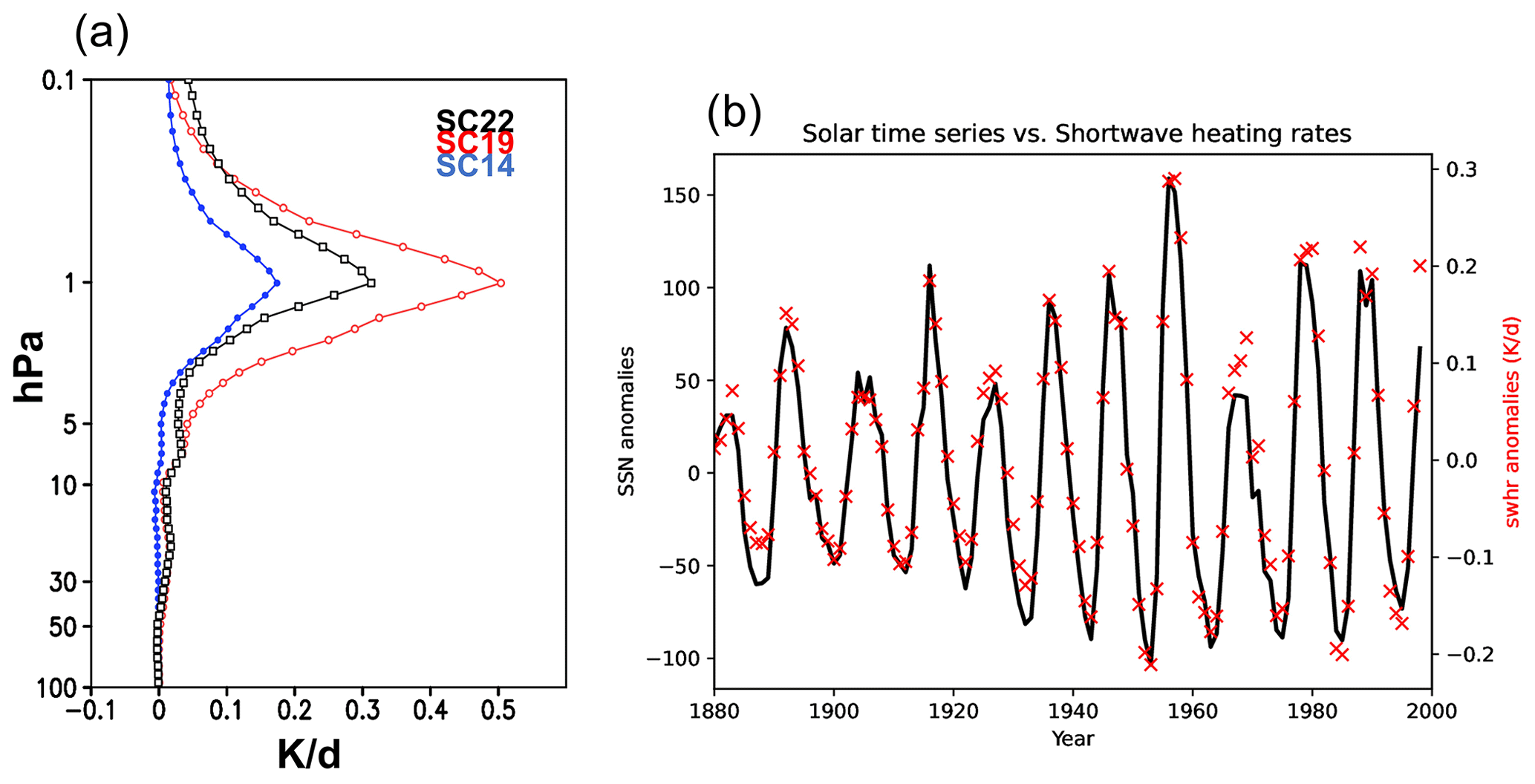
Figure 1 Solar shortwave heating rate signature in the MPI-ESM-HR historical simulations. (a) Tropical annual mean (25^∘ S–25^∘ N) shortwave heating rate difference (in K d⁻¹) between the maximum and minimum of three solar cycles: the weak solar cycle 14 (blue), the medium solar cycle 22 used in CMIP5 (green) and the strong solar cycle 19 (red) (a), as well as time series of the sunspot number and the tropical annual mean (25^∘ S–25^∘ N) shortwave heating rate at the stratopause (1 hPa) (b). Shown are anomalies from a third-degree polynomial fit to the data.

2.2 Data analysis

2.2.1 Detrending, correlations and filtering

To detrend the sunspot number (SSN) (source: WDC-SILSO, Royal Observatory of Belgium, Brussels – https://www.sidc.be/silso/infosnmtot, last access: 1 March 2023) and shortwave heating rate time series, a third-degree polynomial function has been fitted to the data, and the respective anomalies are shown in Fig. 1 (the original, unfiltered SSN time series is shown in Fig. S1 in the Supplement). The detrended SSN time series has then been correlated (Pearson r) with the detrended tropical stratopause temperature (defined as the mean value between 25^∘ S–25^∘ N at 1 hPa; Fig. 3). All correlation analyses have been performed by using the Python scipy.stats.pearsonr function. Statistical significance of the correlations has been calculated by using a two-tailed Student's t test, as implemented in Python. In this paper, we use the term “robust” if a signal of the same sign (e.g., the temperature response at the tropical stratopause) appears in the majority of our ensemble members. To reduce the degree of internal variability, a Butterworth bandpass filter with cutoff frequencies of 9 and 13 years has been applied to the detrended PNJ time series (defined as the arithmetic mean of the zonal-mean zonal wind between 35–45^∘ N at 1 hPa) (Fig. 3). The same Butterworth bandpass filter has also been applied to the zonal-mean zonal wind time series at 10 hPa (zonal mean over 55–65^∘ N) (Fig. 3) and the NAO time series. The NAO time series has been calculated with the aid of an empirical orthogonal function (EOF) analysis conducted for the mean sea level pressure (MSLP) data over the Atlantic sector (20–80^∘ N, 90^∘ W–40^∘ E) in the winter season (DJF averaged and individually for December, January and February). The first principal component is then used to describe the NAO variability. The lead–lag correlations (Fig. 8) are then calculated between the filtered NAO and SSN time series.

2.2.2 Multiple linear regression

To detect the solar cycle signals in the middle atmosphere (Figs. 2, 4 and 5) and in the mean sea level pressure in both observations and model data (Figs. 6 and 7), we use an established multiple linear regression (MLR) technique as described in Bodeker et al. (1998). To derive the individual regression coefficients, we use a set of six predictors in the MLR model:

$$\begin{array}{rl}X\left(t\right)& =\mathrm{Off}.\mathrm{const}+A\times {\mathrm{CO}}_{\mathrm{2}}\left(t\right)+B\times \mathrm{QBO}\left(t\right)\\ & +C\times \mathrm{QBOorth}\left(t\right)+D\times \mathrm{SSN}\left(t\right)+E\times \mathrm{Nino}\mathrm{3.4}\left(t\right)\\ & +F\times \mathrm{tau}\left(t\right)+R\left(t\right),\end{array}$$

with Off.const signifying annual cycle; CO₂(t) signifying increase in the atmospheric CO₂ concentration; QBO(t) signifying phase of the QBO, defined by the zonal-mean zonal wind at 30 hPa (5^∘ S–5^∘ N); QBOorth(t) signifying the orthogonal of QBO(t); SSN(t) signifying SSN time series; Nino3.4(t) signifying Nino3.4 times series; tau(t) signifying optical thickness at 550 nm; and R(t) signifying model residuum. Based on this MLR analysis, we derived the model response to our chosen set of predictors, e.g., the temperature response per unit of the predictor (i.e., K per 1 SSN). To display the model response during solar maximum conditions, we scaled the coefficients to 180 SSN, which is a good approximation for a mean solar cycle amplitude between 1880 and 1999. To detect potential time lags in the response to the solar cycle at the surface, the solar time series has been shifted in such a way that the model response lags the solar forcing by 1 to 4 years. We like to note that we use the raw (unfiltered) model output as input for our MLR analysis.

3 The initial radiative solar signal in MPI-ESM

The dynamical top-down mechanism, assumed to be the pathway for the propagation of the solar signature through the atmosphere to the surface in NH winter (see also Sect. 1), is initiated at the tropical upper stratosphere by the absorption of solar ultraviolet (UV) irradiance by ozone and molecular oxygen. In particular, the absorption of solar photons by ozone in the Hartley bands (200–310 nm) in the upper stratosphere – and to a lesser extent the Huggins bands (310–400 nm) in the middle stratosphere – heats the upper stratosphere increasingly with height and leads to the formation of the warm stratopause. Although the variation in solar UV-irradiance over the 11-year solar cycle is less than 10 % in the ozone absorption bands, the enhanced UV radiation at solar maximum – in combination with increased ozone concentrations – leads to stronger shortwave heating and a concurrent warming of the tropical stratopause on the order of 1 K, as has been derived from merged MSU4 (Microwave Sounding Unit channel 4) and SSU–MLS (Stratospheric Sounder Unit and Microwave Limb Sounder) satellite observations (Randel et al., 2016).

Figure 1a shows the annual mean response of the modeled shortwave radiative heating rate (SWHR) at the stratosphere and lower mesosphere (100–0.1 hPa) for a range of solar cycle (SC) amplitudes, from the weak SC14 (in blue), over the medium SC22 which has been used as solar forcing in the CMIP5 protocol (in green), to the very strong SC19 (in red). MPI-ESM-HR produces the well-known solar cycle impact with enhanced shortwave heating during solar maximum conditions throughout the upper stratosphere and lower mesosphere. The maximum SWHR difference develops at the stratopause and ranges for the three selected solar cycles between 0.17 and 0.51 K d⁻¹. With a SWHR increase of 0.32 K d⁻¹ for the SC22 solar forcing, MPI-ESM-HR produces an initial solar radiative response at the tropical stratopause which is in very good agreement with offline radiation model calculations using the CMIP5 solar forcing (i.e., the same forcing as in MPI-ESM-HR) in a line-by-line reference and two chemistry–climate model (CCM; EMAC and WACCM) radiation codes (see Fig. 8; yellow curves in Matthes et al., 2017). This is a significant improvement compared to the earlier ECHAM4 and ECHAM5 model versions which were not able to simulate the SWHR response to the solar cycle in the stratosphere (see Fig. 17 in Forster et al., 2011) and thus missed the initial solar temperature signal necessary for the top-down mechanism. The improvement in the MPI-ESM-HR is the result of the enhanced spectral resolution of the new shortwave radiation scheme in ECHAM6, which resolves the shortwave spectrum in 14 bands spanning the wavelength range from 820 to 50 000 cm⁻¹ (Iacono et al., 2008), whereas ECHAM4 and ECHAM5 used a lower spectral resolution with the four-band model of Fouquart and Bonnel (1980), later extended to six bands by Cagnazzo et al. (2007).

Figure 1b shows the time series of the SSN and the modeled SWHR at the tropical stratopause over the period from 1880–1999. The shown anomalies of both time series from a third-degree polynomial fit clearly demonstrate that solar cycles of different amplitudes initiate SWHR responses that closely follow in magnitude the strength of the solar forcing. Only during SC20 is the maximum SWHR response higher than expected for that weak solar cycle. This is not reproduced in the SWHR, possibly due to the transition from synthetic SSN before 1979 to observed SSN afterwards.

When averaging over all solar cycles between 1880 and 1999 and all 10 ensemble members, we obtain a robust, highly significant annual mean warming of the complete middle atmosphere at solar maximum (Fig. 2a), reaching a peak response of 1.2 K at the tropical stratopause (Fig. 2b). This result is slightly higher than the solar signal derived from satellite observations (0.7 K per 100 solar flux units, ∼1 K between solar minimum and maximum) (Randel et al., 2016). In our simulations we cannot find the sometimes observed secondary peak in the temperature in the lower stratosphere. This secondary peak, however, can no longer be found even in the most recent analysis of satellite data. Dhomse et al. (2022) suggest that the secondary peak (found in earlier studies) emerged most likely due to aliasing effects related to the Mount Pinatubo eruption in 1991 and probably was not a result of solar variability.

Given the excellent temporal evolution of the initial radiative response of the tropical upper stratosphere to the decadal solar forcing, we conclude that MPI-ESM-HR produces the necessary prerequisite for the dynamically enhanced top-down mechanism, which will be investigated in more detail in the next section.

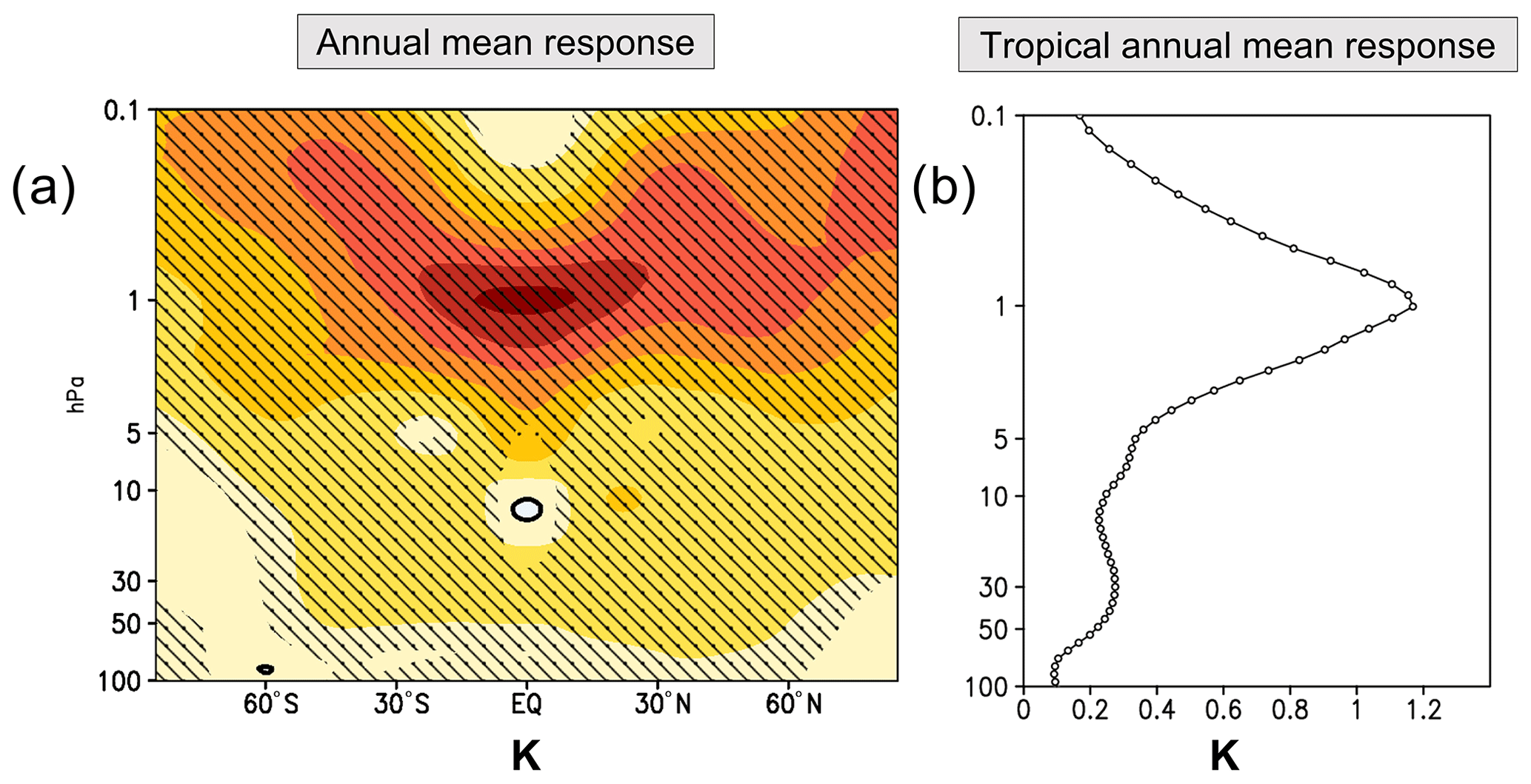
Figure 2 Long-term annual ensemble mean response based on MLR analysis of the zonal-mean temperature (in K) to the solar cycle in the middle atmosphere as a function of height and latitude (hatched regions mark 95 % statistical significance) (a) and the tropical annual mean (25^∘ S–25^∘ N) temperature response (in K) (b).

4 Downward transfer of the solar signal to the surface: the key role of dynamics

After having demonstrated the ability of the MPI-ESM-HR model to realistically simulate the radiative and the related temperature response in the tropical upper stratosphere to the decadal solar forcing, we investigate as the next step the potential dynamical reaction to the radiative forcing, which is expected according to the top-down mechanism. By evaluating the ensemble spread in the NH during the dynamically active season (November to March), we assess the variability in different dynamical variables in the stratosphere with respect to the solar fluctuations in the MPI-ESM-HR historical ensemble simulations. We focus first on the detrended deviations from the long-term monthly means for the TST and (to estimate the dynamical response in the NH) the zonal-mean zonal wind at two different altitudes and latitudes (Fig. 3). To approximate the PNJ (the local maximum wind speed in the upper stratosphere), we use the mean of the zonal-mean zonal wind in 35–45^∘ N at 1 hPa. The variability in the middle stratosphere is represented by the mean of the zonal-mean zonal wind in 55–65^∘ N at 10 hPa. After calculating the respective anomaly time series for the TST, the PNJ and the 10 hPa zonal wind variations for each month individually, we correlate these time series with the detrended DJF mean SSN time series. To mute the interannual variability (operating on timescales between 1 and 8 years) of the polar vortex, the PNJ and 10 hPa anomaly time series, as well as the SSN time series, have been bandpass-filtered before the correlations are calculated. Please note that the same SSN time series has been used for the correlation for all individual ensemble members, leading to a “vertical arrangement” of the data in the scatter plots shown in Fig. 3. Our results indicate that the TST correlates significantly with the SSN, not only in the annual mean (see Fig. 1b) but also in each individual month considered (Fig. 3, left column). While negative and positive TST anomalies (i.e., negative and positive deviations from the long-term monthly mean) are almost uniformly distributed for SSN values smaller than the SC14 maximum (dotted blue lines), an increase in the solar forcing exceeding the SC14 SSN maximum leads to a higher probability of positive TST anomalies. The strength of the correlations changes over the season such that a stronger connection between the solar forcing and the temperature response at the tropical stratopause is given in late autumn (November: r=0.28) and late winter (February: r=0.34; March: r=0.42). In these months, a particularly strong solar forcing (indicated by the SSN value of the SC19 maximum; dotted red lines) is almost always associated with a positive temperature anomaly at the tropical stratopause. Weaker correlations and a broader distribution of negative and positive temperature anomalies, even during periods with especially pronounced solar activity, are calculated for the midwinter season (December: r=0.15; January: r=0.16). These findings are consistent with an increase in the overall variability in the TST during December and January, making it more difficult for the relatively weak solar-induced signals to be distinguished from the background noise. The higher variability in the TST during December and January is probably a result of the higher variability in the tropical branch of the Brewer–Dobson circulation (BDC) in boreal winter (e.g., Butchart, 2014).

According to the general concept of the top-down mechanism the initial signal in the TST would be accompanied by a strengthening of the PNJ via a modification of the meridional temperature gradients. Considering the statistically significant temperature signals and correlations at the tropical stratopause in the MPI-ESM-HR model (Fig. 3, left column), we expect a dynamical response of the PNJ in our simulations. However, the correlations between the SSN and the PNJ time series (Fig. 3, middle column) do not show statistically meaningful relations between the solar forcing and the dynamical response of the PNJ. Only during February is a weak but statistically significant correlation found, which might be related to the enhanced impact of the solar forcing in the TST during the same month. However, this connection as well becomes insignificant if the correlations are calculated based on the unfiltered SSN and PNJ time series. Figure 3 (right column) shows the correlations between the solar forcing and the zonal-mean zonal wind for the lower (and more northward) 10 hPa anomaly time series. We find the strongest (and significant) correlations in November (r=0.25) and December (r=0.13), although these correlations become (again) negligible if the correlations are calculated based on unfiltered model data. The differences in the timing between the maximum correlations of the SSN with the PNJ (February) and the 10 hPa zonal wind time series (November and December) are not in line with the established idea of a successive “poleward and downward” progression of the dynamical solar signal. Furthermore, the computed SSN–PNJ correlations for November, December, January and March are ≤0.06, implying that the characteristics of the PNJ are not markedly influenced by the magnitude of the solar forcing and thus the amplitude of the solar cycle.

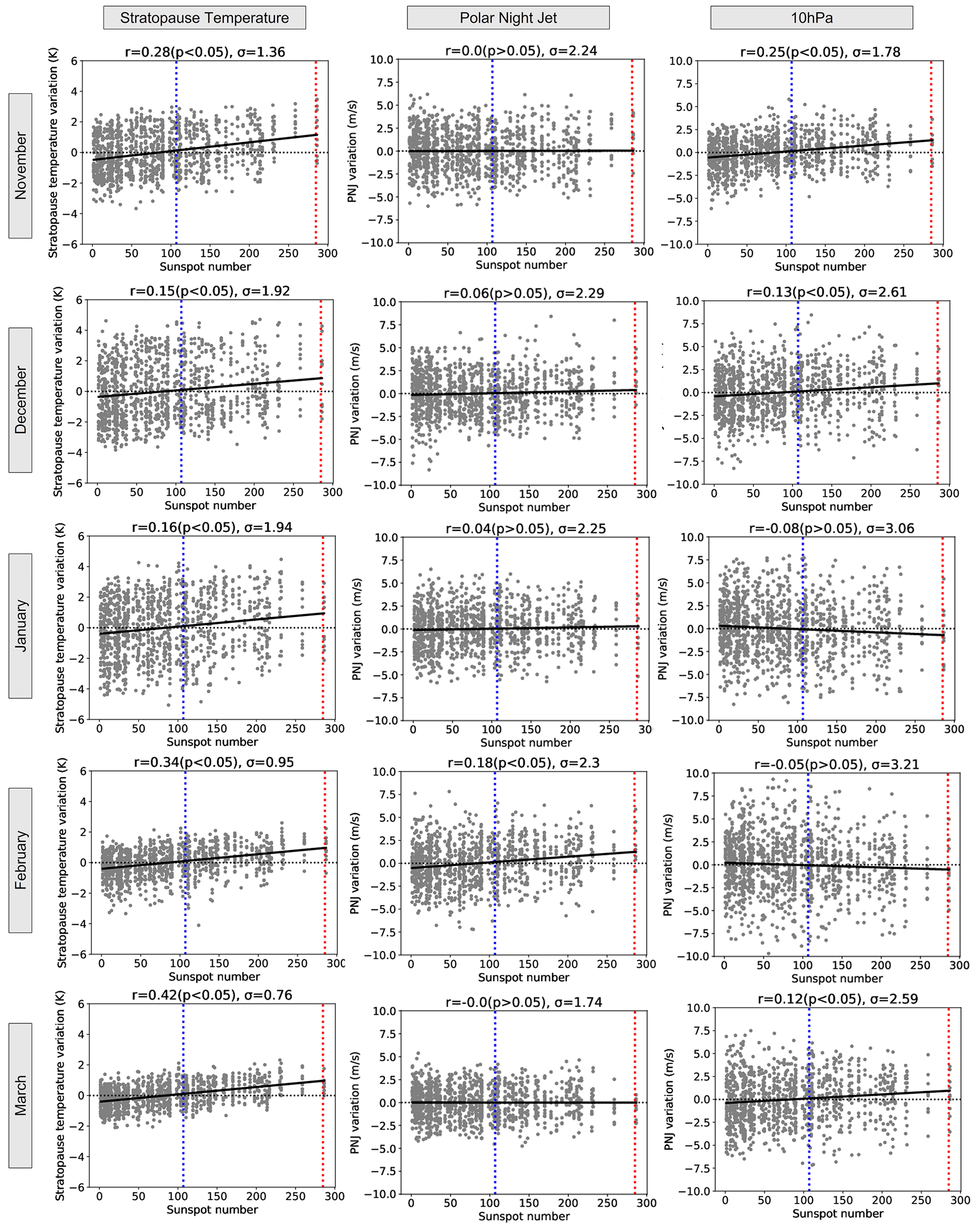
Figure 3 Scatter diagram of variations vs. SSN of the stratopause temperature (left column), PNJ (middle column) and zonal-mean zonal wind averaged over 55–65^∘ N at 10 hPa (right column). The numbers given in the headings show the correlation coefficients (r), their statistical significance (p<0.05: significant correlation; or p>0.05: insignificant correlation) and the overall variation (σ). The dotted blue and red lines indicate the SSN at solar cycle maximum for SC14 and SC19 (the weakest and strongest solar cycles considered in the simulations).

Figure 3 demonstrates that while the connection between the solar forcing and the TST is clearly visible in our correlation analysis, the potential dynamical response in the NH is harder to detect, especially due to the highly variable polar vortex. Therefore, we proceed using an MLR analysis to separate the potential dynamical solar-induced signals from other internally generated disturbances in the ensemble mean.

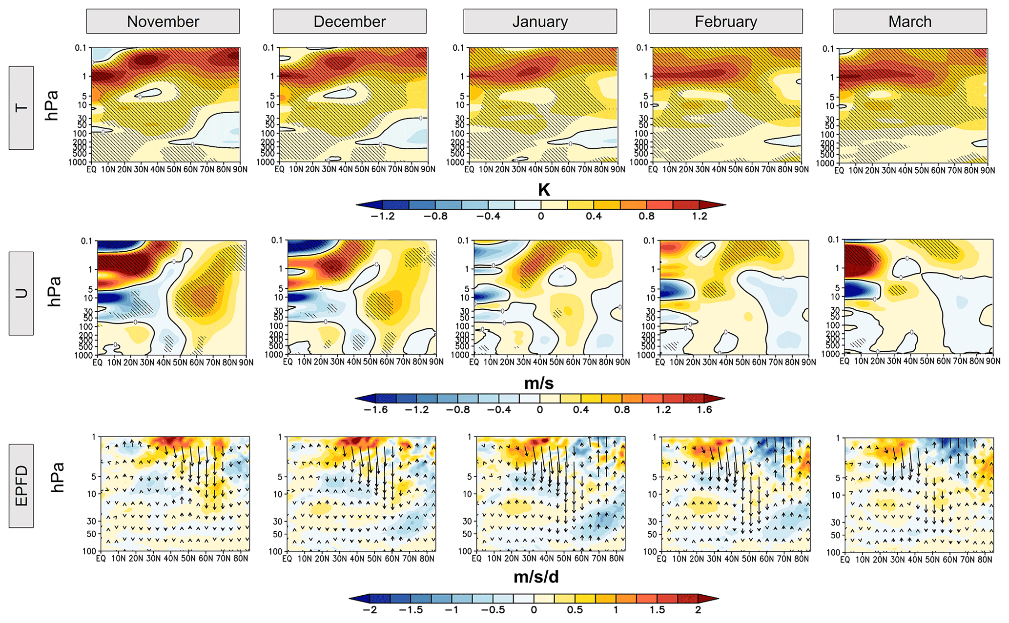
Figure 4 The ensemble mean long-term response (based on MLR) to the solar cycle of the zonal-mean temperature (first row), zonal-mean zonal wind (second row) (hatched regions mark 95 % statistical significance), and the EPF (vectors) and the divergence of the EPF (EPFD, colors) in the NH during the boreal winter season. All results have been scaled to 180 SSN.

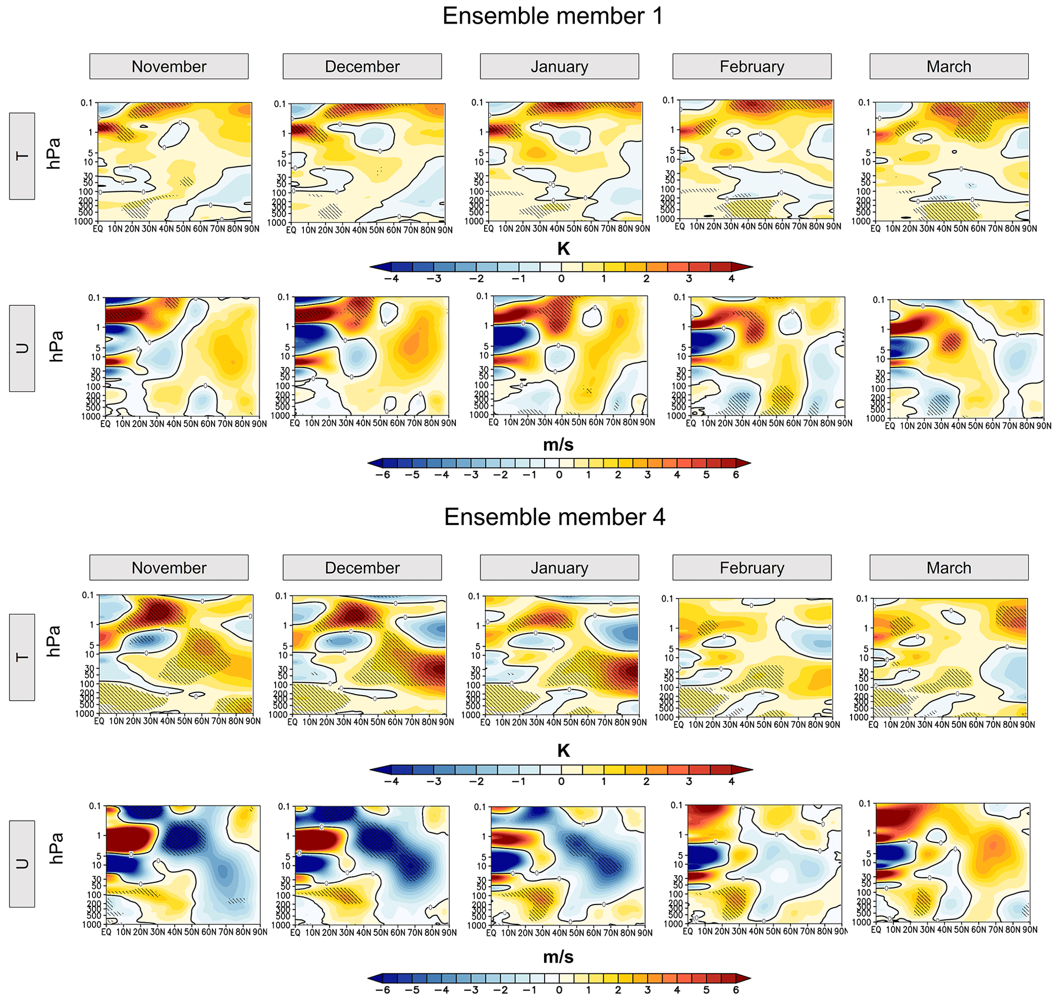
Figure 5 Long-term response (based on MLR) to the solar cycle of the zonal-mean temperature (first row) and the zonal-mean zonal wind (second row) (hatched regions mark 95 % statistical significance) in the two ensemble members EM1 (top panels) and EM4 (bottom panels) in the NH during the boreal winter season. All results have been scaled to 180 SSN.

After having analyzed the variability in the TST, the PNJ and the 10 hPa zonal-mean zonal wind, we will now isolate potential solar signals with the aid of MLR. Figure 4 shows the solar regression coefficients, scaled to a mean amplitude of the solar cycle (180 SSN), for the zonal-mean temperature (top row), the zonal-mean zonal wind (middle row), and the EPF (vectors) and its divergence (EPFD; colors) (bottom row) for each NH winter month (November–March). Here, we focus on the potential solar cycle signals between the Equator and the North Pole and pressure heights at 1000–0.1 hPa for the temperature and wind responses and 100–0.1 hPa for the EPF diagnostics. We find a significant response in the zonal-mean temperature at the tropical stratopause (Fig. 4, top row) with a maximum response at the Equator of 1.2 K during November. The solar-induced temperature signal is confined to the inner tropics in late autumn and early winter and advances towards higher latitudes between January and March. This is consistent with the seasonal march of the incidence angle of solar radiation after the winter solstice in December. In the middle to polar latitudes, we find a clear dipole in the temperature anomalies especially during November and December. This dipole is characterized by distinct (and significant) positive temperature anomalies in the lower mesosphere and upper stratosphere and weak (and insignificant) negative anomalies in the middle and lower stratosphere. Particularly the pronounced polar heating in the upper stratosphere from November to December agrees well with a more recent analysis of ERA-Interim reanalysis data by Kuroda et al. (2022). The detected temperature signals in the middle atmosphere in November and December are in line with the anomalies in the zonal-mean zonal wind (Fig. 4, middle row), which indicate a stronger (and thus cooler) polar vortex during these months. Additionally, a convergence of the EPF (indicated by the reddish colors in Fig. 4, bottom row) and its (here downward-oriented) vectors imply a reduced upward propagation of planetary waves due to the strengthening of the polar vortex. The maximum (and significant) response in the stratospheric zonal-mean zonal wind in the area of the polar vortex is located at ∼ 60^∘ N at 10 hPa. Here, we find positive anomalies of the zonal-mean zonal wind of ∼1 m s⁻¹. Given the zonal-mean wind speeds between 20 m s⁻¹ (November) and 30 m s⁻¹ (December), simulated by the model (not shown) at this height and latitude, the solar influence seems rather small in comparison. The detected dipole in the zonal-mean temperature starts to weaken from January on and vanishes almost completely until March. During the same months, we find a (yet insignificant) weakening of the polar vortex which allows for more upward propagation of planetary waves (indicated by a divergence of the EPF (bluish colors) and upward-oriented vectors). In the troposphere, a weak (≤0.5 m s⁻¹) but significant westerly wind anomaly around ∼ 60^∘ N can be detected in November and December. The weak tropospheric wind response agrees with other studies (Matthes et al., 2006; Schmidt et al., 2010; Ineson et al., 2011; Chiodo et al., 2012; Langematz et al., 2013; Kuroda et al., 2022; Drews et al., 2022).

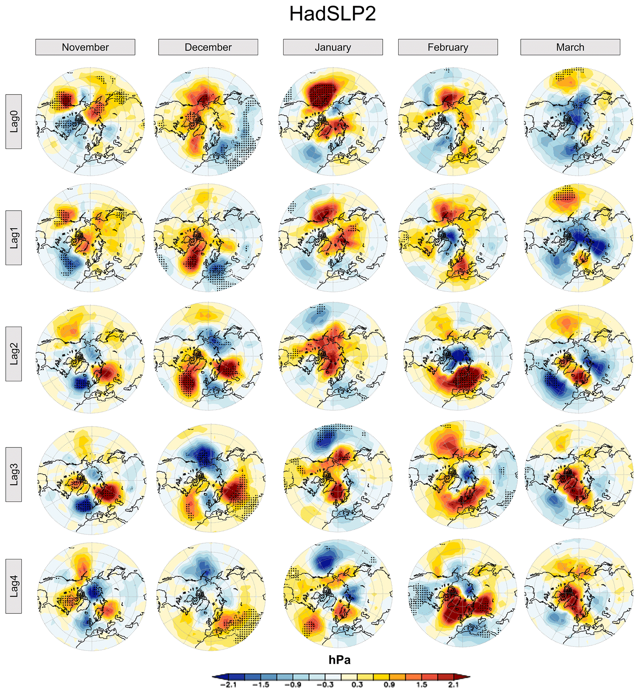
Figure 6 The (lagged) response of mean sea level pressure (MSLP) to the solar cycle in the NH during the boreal winter season for the HadSLP2 dataset (dotted regions mark 95 % statistical significance). Columns denote the individual months of the winter season; rows indicate the lag of the MSLP time series with respect to the solar forcing time series.

While in some studies the march of the westerly wind anomalies from the middle atmosphere to the surface seems to follow the proposed “poleward and downward” concept (e.g., Matthes et al., 2006; Ineson et al., 2011; Drews et al., 2022), the signal transmission in the MPI-ESM-HR and other model simulations (e.g., Schmidt et al., 2010; Chiodo et al., 2012; Kuroda et al., 2022) rather follows a “downward-only” storyline. Additionally, the description of the westerly wind anomalies at the surface is sometimes inconsistent with the idea of a successive downward propagation of the signal from higher to lower altitudes. As an example, significant westerly wind anomalies at the surface at middle latitudes are already present in November in the modeling studies of Matthes et al. (2006) and Kuroda et al. (2022), even though the major signal is still high up in the middle atmosphere. Furthermore, in Kuroda et al. (2022) the westerly wind anomalies at the surface at middle latitudes are present throughout the complete season (i.e., in all months between November–March), similar to our MPI-ESM-HR simulations. In other studies, the westerly anomalies are insignificant (e.g., Schmidt et al., 2010) or do not reach the ground (e.g., Chiodo et al., 2012). This implies that the detected surface wind anomalies could be independent from the seasonal march in the middle atmosphere and might rather be a product of the internal variability in the troposphere (i.e., the AO or NAO) itself. Likewise, the temperature response to the solar cycle in the troposphere with positive temperature anomalies of ≤ 0.2 K at the surface is rather weak (Fig. 4, top row). Interestingly, these small temperature signals are significant in the tropics in all considered months, which is consistent with the high (and relatively constant) solar insolation in the inner tropics and a damped overall variability compared to the extratropical regions. By contrast, the significant surface temperature anomalies in the extratropical regions are located between 50 and 60^∘ N until January and shift towards the polar latitudes in February and March.

So far, we focused on the discussion of the potential solar signals in the ensemble mean derived from the 10 individual MiKlip historical simulations, thus obtaining statistically more robust results than is possible through analyses of single simulations. The necessity of working with ensemble mean results is impressively demonstrated by comparing 2 of our 10 individual ensemble members. Figure 5 shows the solar regression coefficients for the zonal-mean temperature and zonal-mean zonal wind for ensemble members 1 (EM1, top panel) and 4 (EM4, bottom panel), as in Fig. 4. The derived patterns for the zonal-mean solar temperature signal in EM1 show distinct similarities to the ensemble mean. As an example, we find a (significant) maximum temperature response around the tropical stratopause. Furthermore, the distribution of the temperature anomalies in the middle to higher latitudes again displays the polar heating in the lower mesosphere and the upper stratosphere and the cooling in the middle to lower stratosphere. Again, this pattern starts to weaken from January on. We notice that in comparison to the ensemble mean, fewer areas depict significant temperature signals, even though the magnitude of the temperature response is stronger. This can be attributed to the fact that the analysis only includes 120 model years and thus ∼12 solar cycles (instead of 1200 and ∼120 in the ensemble mean), which are seemingly not enough to dampen the internal variability and inhibit the solar-induced signals from becoming significant against the overall background noise. Likewise, the solar response of the zonal-mean zonal wind in the middle atmosphere in EM1 shows the main characteristics, as already noticed in the ensemble mean, such as a strengthening of the polar vortex in November and December, a subsequent weakening, and a conversion in sign afterwards. However, none of the detected signals in the area of the polar vortex is statistically significant. As for the response of the zonal-mean zonal wind at the surface, we detect significant anomalies in January and February. The geographical distribution of the anomalies (westerly wind anomalies at middle latitudes and easterly wind anomalies at polar latitudes), however, mimics a negative phase of the AO which is not in line with the general concept of solar-induced top-down influences.

In EM4, the initial temperature signal in the tropical upper stratosphere is, as in EM1, visible throughout the complete season and the strongest in November and December. Thus, the response to the solar cycle at these latitudes and heights turns out to be a robust feature in the MPI-ESM-HR model experiments. However, even though exactly the same solar forcing has been applied in EM4 as in EM1, the initial temperature signal is not significant (most likely due to the individual internal variability in this ensemble member), and the dynamical response of EM4 in the extratropical regions looks very different. For instance, we find a cooling of the polar upper stratosphere and a (significant) warming in the middle to lower stratosphere in December and January. This pattern is common during SSWs, which (by chance) could have been more frequent in EM4 during December and January than in EM1. The strong and significant easterly wind anomalies in the middle atmosphere, indicating a slowdown of the polar vortex during these months, underpin this hypothesis. These findings imply that the detected signals in EM1 could also be a result of (by chance) less frequent SSWs in EM1, leading to a potentially misleading attribution to solar variability. In our simulations, 4 out of 10 simulations show a weakening of the polar vortex during high solar activity, while six depict a strengthening of the latter, which may explain the rather weak tendency to westerly wind anomalies in the ensemble mean.

Either way, our results point to the fact that the internal dynamics of the polar vortex have the ability to control the transmission of potential solar-induced signals from the tropics to the polar regions and are thus more important than the amplitudes of individual solar cycles (see also Fig. 3), as recently claimed by Drews et al. (2022).

5 Direct and lagged surface solar signals

Our results so far indicate a robust response of the TST to the quasi-decadal solar cycle. The subsequent dynamical response in the NH during the boreal winter season, however, is difficult to assess. With the aid of an MLR analysis we could detect weak solar cycle imprints in the zonal-mean temperature and the zonal-mean zonal wind in the ensemble mean. However, these signals are not robust among all individual ensemble members, especially with respect to the detected anomalies in the zonal-mean zonal wind at the surface which seem to be independent of the signals in the middle atmosphere.

Nevertheless, in the next step, we first aim at detecting potential solar signals at the surface by applying the MLR analysis to mean sea level pressure (MSLP) data in NH winter. Figure 6 shows the monthly solar regression coefficients for MSLP, scaled to a mean solar cycle amplitude of 180 SSN, in the HadSLP2 observational dataset (Allan and Ansell, 2006) for the same period as simulated (1880–1999). In order to check for eventual time lags between the applied solar forcing and the model response, as suggested for example by Gray et al. (2013), lagged regressions were calculated by shifting the solar predictor time series against the observations so that it leads the model data between 1 and 4 years. Our results show positive and negative anomalies in the MSLP in the middle and polar latitudes which mimic positive and negative phases of the AO in a rather more random than systematic way. As an example, we find an AO-positive-like pattern (i.e., negative pressure anomalies over the North Pole and positive pressure anomalies in the surrounding middle latitudes) in November at lag year 4, in December at lag year 4, in February at lag years 1 to 3 and in March at lag year 1. The most pronounced AO-positive anomalies, with a negative but insignificant anomaly of ∼2 hPa over the North Pole and a positive anomaly of the same magnitude in the middle latitudes, are given at lag year 2. Hence, the strength of the detected potential solar signals in our HadSLP2 analysis is in line with other studies assessing observational products (e.g., Gray et al., 2013; Kuroda et al., 2022; Drews et al., 2022). The detected maximum impact at lag year 2 in February in our analysis, however, agrees with Kuroda et al. (2022) and Drews et al. (2022) but differs from Gray et al. (2013), who found a maximum response at lag year 4 in the DJF mean. These discrepancies in the timing of the peak solar-induced surface signal in the HadSLP2 MSLP data can only be explained by differences in the analysis techniques, and they reveal a high sensitivity of solar-induced surface signals to the applied methodology and individual interpretation of the results. Furthermore, due to the lack of data covering the whole atmospheric domain over the complete historical period, it is not possible to connect the potential surface solar signals to the seasonality in the middle atmosphere. This applies to our study and the original studies (e.g., Gray et al., 2013).

Figure 7 shows the same analysis for the MiKlip historical simulations, i.e., the ensemble mean of the solar regression coefficients for the MSLP for each month (November to March) and (lag) years 0 to 4. We detect AO-positive-like anomalies in the MSLP in December at lag years 0 and 1, in January at lag years 0 to 4, and in February at lag years 0 to 4. The strongest negative MSLP anomalies over the North Pole show a response of ∼ −1.5 and $\sim +\mathrm{1.5}$ hPa in the middle latitudes in January and December. Thus, the overall model response is weaker compared to the observational data. This is not surprising given the fact that the model results depict the mean over 10 ensemble members (with respective dampening effects) compared to one “ensemble member” representing the observations. While the detected magnitudes of the MSLP anomalies in MPI-ESM-HR agree with other solar cycle model studies (e.g., Gray et al., 2013; Scaife et al., 2013; Andrews et al., 2015; Drews et al., 2022), the detected timing (i.e., the progression of the signals from the middle atmosphere to the surface) in the MPI-ESM-HR does not fit the narrative of the top-down mechanism as described most recently by Kuroda et al. (2022) and Drews et al. (2022). In these studies, the authors find the most pronounced AO-positive-like pattern in February at the surface and link this to the coupling between the stratosphere and the troposphere, which peaks in exactly this month. In contrast, in our model simulations the strongest coupling between the stratosphere and the troposphere appears in December (see Fig. 4), while the most pronounced AO-positive-like patterns appear in January and February at different lag years. Statistical studies based on MLR analysis of observed and reconstructed MSLP data find both NAO signals in early and late winter at different lags (Grey et al., 2016; Ma et al., 2018). We, therefore, conclude that the detected surface solar signals could rather be a product of the internal variability in the troposphere itself than being necessarily a consequence of the proposed top-down mechanism. Even if we assume that the detected surface signals have a pure solar source (and the top-down mechanism is always present during solar maximum years), it seems to be questionable in our view that these tiny signals would have the capability to synchronize powerful large-scale climate modes such as the AO or the NAO if they only emerge once per decade over the duration of a month. As an example, the Icelandic Low and the Azores High, both controlling the pressure gradients in the North Atlantic sector, show a month-by-month variation of ∼8.5 and ∼6 hPa during winter time in the model (not shown).

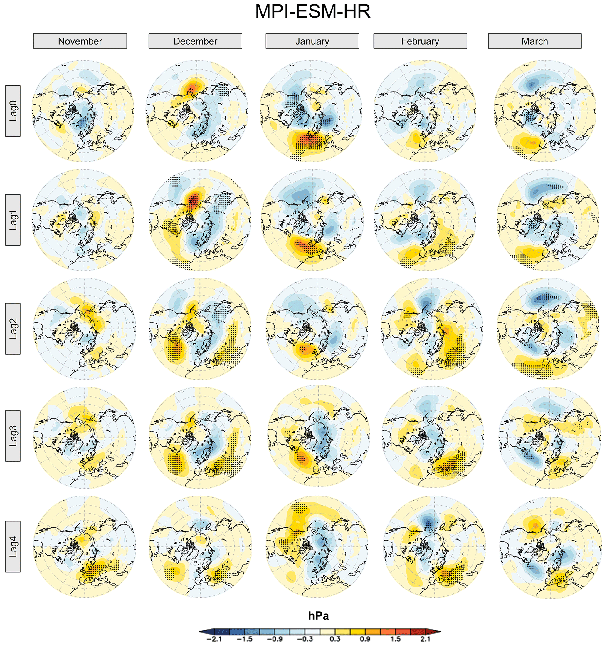
Figure 7 As Fig. 6 but for the ensemble mean of the MPI-ESM-HR MiKlip historical simulations.

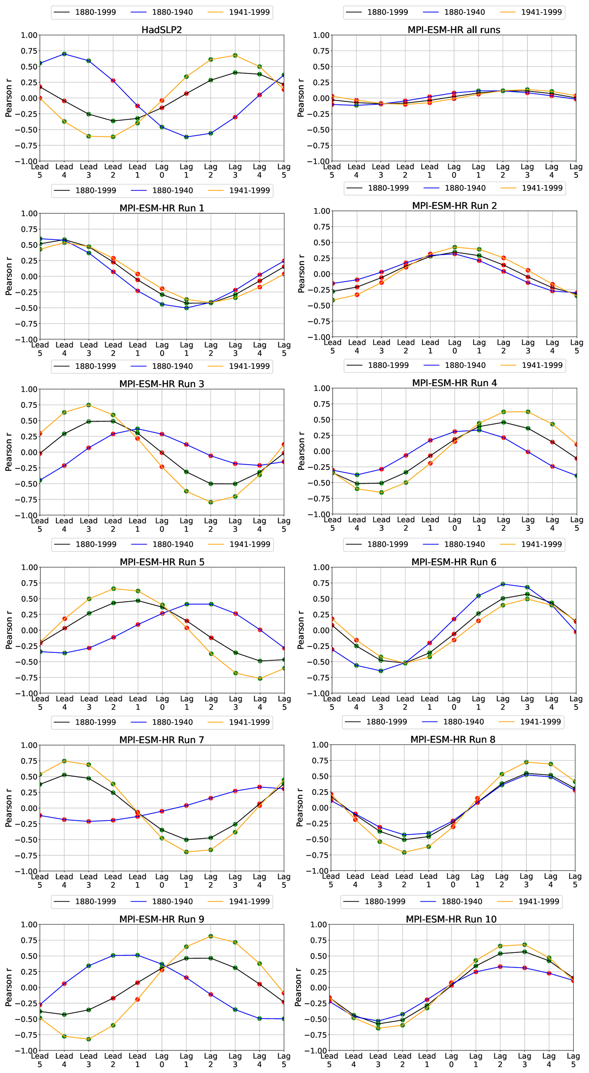
Figure 8 Lead–lag correlations between the seasonal mean (DJF) bandpass-filtered PC1 based on NAO and SSN time series for the HadSLP2 dataset and the ensemble mean of the MPI-ESM-HR historical simulations (top row) and the individual MPI-ESM-HR historical runs (rows two to six) for different periods. Green dots mark statistically significant (95 %) correlations.

6 A synchronization of the NAO by the solar cycle?

In the following, we will address the question of if the quasi-decadal variations in the solar cycle have the ability to synchronize the decadal component of the NAO, as proposed by Thiéblemont et al. (2015) and Drews et al. (2022). For a better comparison, we apply the same analytical strategy as proposed by Thiéblemont et al. (2015) to our model simulations and the HadSLP2 data, however with the exception that we use the SSN instead of the F10.7 solar flux times series as a solar proxy. Since both the SSN and F10.7 time series show the same oscillations on the interannual and decadal timescales, this is irrelevant for the interpretation of the results. First, an EOF analysis is applied to the deseasonalized MSLP data over the Atlantic sector (20–80^∘ N, 90^∘ W–40^∘ E) in the winter season (DJF averaged). Before continuing, we compared the spatial pattern of the EOF analysis between the modeled and observed data and found good agreement with respect to the centers of action and overall characteristics (not shown). The resulting leading principal components (PC1) are then used to describe the variability in the NAO. To mute major parts of the interannual variability, we apply a Butterworth bandpass filter with cutoff frequencies of 9 and 13 years to the PC1 and the SSN time series. As a result, the filtered PC1 and SSN time series only include the oscillations operating on the quasi-decadal timescale. Subsequently, lead–lag correlations are calculated between the bandpass-filtered PC1 and SSN time series for both the complete dataset and all individual ensemble members (1 to 10). Drews et al. (2022) recently argued that the correlations would become more meaningful during the course of the 20th century due to a series of solar cycles with stronger amplitudes. We, therefore, compute the correlations for three different time segments: the whole period (WP) (1880–1999), the early period (EP) with weaker solar amplitudes (1880–1940) and the late period (LP) with more pronounced solar amplitudes (1941–1999).

For the HadSLP2 dataset (Fig. 8, left column, first row) positive correlations between the decadal variation in the NAO and the solar forcing are found for lag years 1 to 4 in both the WP and the LP periods, with maximum correlations at lag year 3 during the LP. For the EP, we find an out-of-phase relation between the solar time series and the NAO on the decadal timescale. The evaluation of this (one ensemble member) observational dataset implies that the solar forcing actually leads the surface response by a couple of years and that this relation is more pronounced during phases of higher solar activity. Indeed, similar phase relations in the different time segments are given by individual ensemble members of the MiKlip historical simulations (e.g., EM9; Fig. 8, left column, sixth row). However, phase relations like these seem far from being a robust feature if all model runs are considered. As an example, EM5 (Fig. 8, left column, third row) indicates positive correlations between the decadal behavior of the SSN and the NAO time series for lag years 1 to 3 during the EP, while this relation reverses (showing negative correlations) during the WP and LP. This is also true for EM3 (left column, third row) and EM7 (left column, fifth row). Other ensemble members (EM2; Fig. 8, right column, second row) suggest a maximization of the solar impact at lag year 0 and this independently of the considered period. Furthermore, EM6 (Fig. 8, right column, fourth row) indicates stronger positive correlations at positive lag years during the EP than during the LP. The most striking discrepancies, however, come from EM1 (Fig. 8, left column, second row) and EM4 (Fig. 8, right column, third row). While EM1 shows negative correlations between the solar forcing and the NAO at positive lags (in all time segments), this is the opposite in EM4. These surface responses in EM1 and EM4 are, however, opposite to what would be expected from the polar vortex responses in these two ensemble members (a pronounced strengthening of the polar vortex and a downward propagation of westerly wind anomalies to the surface in EM1 and a weakening of the polar vortex and a downward propagation of easterly wind anomalies to the surface in EM4 during winter; see Fig. 5) and opposite to the top-down mechanism.

When applied to the complete dataset of the MiKlip historical simulations, the correlation analysis yields a weak positive (albeit significant) correlation at lag years 2 to 4, rather independently of the considered time segment. This, however, should rather be interpreted as a slight (and by chance) overhang to positive correlations in the MiKlip dataset (that could change in a larger ensemble) than a robust physical connection between the solar forcing and the NAO. To verify whether the use of the seasonal mean (DJF) might dampen the solar cycle response, as discussed by Drews et al. (2022), we repeated the analysis for the individual winter months (December, January and February; see Fig. S2 in the Supplement) for the model data. We did not detect stronger connections between the decadal solar forcing and the NAO in the calculations based on individual months compared to the seasonal mean. On the contrary, the correlation analysis based on the December months (i.e., the month where we find the “strongest” top-down signals in the middle atmosphere) depicts negative correlations at positive lag years. In summary, given all of these inconsistencies we suspect that there is no robust connection between the quasi-decadal solar oscillations and the respective phase of the NAO in the CMIP5 MiKlip historical ensemble simulations.

7 Summary and discussion

Our analysis of the MiKlip historical ensemble simulations, conducted with the state-of-the-art Earth system model MPI-ESM-HR, revealed robust (and statistically significant) solar signals in the TST (see Figs. 1 and 2). The dynamical responses to the initial solar temperature signal at the tropical stratopause, in the NH middle to polar latitudes during the boreal winter season, however, showed a large spread among our data. This applies to the variability in the PNJ and the 10 hPa zonal-mean zonal wind time series, which both did not show meaningful correlations with the solar forcing (see Fig. 3). When removing components other than decadal variability from MLR analysis, we were able to detect (albeit rather weak) solar signals in the NH winter, in both the ensemble mean zonal-mean temperature and zonal-mean zonal wind, that basically agree with the proposed top-down influence of solar variability in the middle atmosphere (see Fig. 4). However, the MLR analysis based on individual ensemble members revealed signals of opposite directions (i.e., a strengthening (EM1) or weakening (EM4) of the polar vortex during periods of high solar activity) (see Fig. 5). Furthermore, we find indications that the detected anomalies in the zonal-mean zonal wind at the surface are most likely independent of the signals in the middle atmosphere. The alleged surface solar signals in MSLP seem to mimic AO-positive (and AO-negative) patterns randomly rather than in a systematic way. This applies to the HadSLP2 data (Fig. 6) and to the model data (Fig. 7), which both depict a very pronounced AO-positive pattern in January and February at different lag years, however in months when the strong stratospheric influence (in December) is already weak or even reverses sign in the model (see Fig. 4). With respect to the suggested synchronization between the decadal solar forcing and the NAO (e.g., Thiéblemont et al., 2015), we cannot find any meaningful relations in the MiKlip historical simulations. This is supported by the fact that all ensemble members show very individual phase relations (i.e., positive/negative correlations and maximizations during different lag years) between the solar and the NAO time series. Additionally, more robust correlations could not be achieved in different time segments (i.e., periods with stronger or weaker solar forcing). These findings apply to the seasonal winter mean (DJF), as well as to individual winter months (December, January and February). As a consequence, the detected phase relations in the HadSLP2 dataset should be interpreted carefully with respect to potential physical connections between the solar forcing and the NAO, in particular since the observations represent only one single ensemble member.

In summary, we draw four major conclusions:

1. The decadal variations in the TST in the MiKlip historical simulations are a product of the 11-year solar cycle. In the course of this, an increase in the solar intensity leads to enhanced radiative shortwave heating rates and a warming of the TST. These findings are consistent with other modeling studies concerning the imprints of the 11-year solar cycle in the tropical upper stratosphere (Matthes et al., 2004, 2006; Schmidt et al., 2010; Ineson et al., 2011; Chiodo et al., 2012; Langematz et al., 2013). The solar signals in the TST are statistically significant and robust and were detected by our correlation and MLR analyses.

2. The dynamical response of the NH during winter in the middle atmosphere shows a weak strengthening of the polar vortex during solar maximum conditions in the ensemble mean in the MLR analysis. However, the signals (especially in the zonal-mean zonal wind) are mostly insignificant and of opposite sign in individual ensemble members and are thus not a robust feature. We suppose that the dynamical background state in the middle atmosphere (i.e., the variability in the polar vortex) seems to play an important role in the transfer of the initial radiative solar signal from the tropical upper stratosphere down to the troposphere in NH winter. The important role of middle-atmosphere dynamics in modulating potential solar signals is currently being investigated as part of the SOLCHECK project and will be published in a subsequent paper (Wenjuan Huo, personal communication, 2023).

3. The detected anomalies in the zonal-mean zonal wind and MSLP at the surface seem not to be related to the timing of the seasonal march of the signals in the middle atmosphere and are most likely a manifestation of the internal variability in the troposphere itself.

4. Concerning the decadal variations in the NAO and the solar forcing, our results suggest that both are independent from each other. We find a range of phase relations between the NAO and the solar forcing throughout our ensemble members, which implies a random statistical relation rather than a physically sound connection.

It should be noted that we did not explicitly analyze a potential TSI-controlled bottom-up effect on the surface solar signal, as bottom-up effects are rather confined to tropical latitudes with a prolonged influence of the TSI throughout the year (e.g., Meehl et al., 2008). Moreover, potential effects related to energetic particle precipitation are not explicitly included in the MiKlip experiments. Since these effects are known to be rather small and even less understood than the 11-year solar cycle surface imprints, we do not think they would alter our results significantly (please see the Introduction section).

Since the critical study of Chiodo et al. (2019), the top-down mechanism and its surface imprints have been further discussed in the scientific community. It is unquestionable that early studies with GCMs and CCMs found evidence of a top-down mechanism in the middle atmosphere which in most cases penetrated into the troposphere in NH winter (Matthes et al., 2004, 2006; Schmidt et al., 2010; Ineson et al., 2011; Chiodo et al., 2012; Langematz et al., 2013). These studies all reproduced more or less the basic features of the top-down mechanism, thus confirming the physical mechanisms at work suggested by Kodera and Kodera (2002). In contrast, more recent simulations with CCMs and ESMs do not seem to find statistical responses of surface variables to the decadal solar forcing (e.g., Chiodo et al., 2019; this study). Only Drews et al. (2022) showed a solar near-surface imprint for solar cycles with strong amplitudes. The MiKlip simulations are more in line with Chiodo et al. (2019), who argued that the alleged solar surface signals could be an incidental product which is only detectable during phases with stronger solar cycles. Our results even suggest that robust solar surface imprints are basically absent throughout the complete historical period and are thus not sensitive to the amplitude of individual solar cycles. At this point we would like to emphasize that in contrast to previous studies, the MiKlip simulations represent a transient climate system driven by a realistic (observed) solar forcing, thus enhancing the confidence in a comparison of our model results to observations.

We suggest that the gradual “fading away” of significant solar near-surface signatures in more up-to-date model studies is closely related to progresses made in model development and computer capacities allowing for ensemble simulations. The early simulations were conducted with fixed lower-boundary conditions (i.e., prescribed sea surface temperatures (SSTs) from observations or control run experiments) (Matthes et al., 2006; Schmidt et al., 2010; Chiodo et al., 2012). Some applied perpetual conditions for the solar forcing (i.e., perpetual solar maximum vs. perpetual solar minimum) and steady-state conditions for the greenhouse gas forcing (Matthes et al., 2006; Schmidt et al., 2010; Ineson et al., 2011). While these models included the necessary physical mechanisms, i.e., UV radiation codes and middle-atmosphere dynamics, to capture the solar UV-induced top-down solar signal, the complex nature of physical and chemical processes and the spectrum of internal variability were reduced. Prescribed SSTs, for example, prevent the model from developing the complete spectrum of interannual variability in the troposphere (e.g., induced by the internal variability in the NAO), which might counteract potential surface solar signals. In addition, steady-state background conditions in atmospheric greenhouse gas concentrations and prescribed ozone-depleting substances do not take into account transient adjustment processes in the atmospheric dynamics, which again lead to a reduction in the overall internal variability and maybe an overestimation of solar-induced signals. Moreover, due to more limited computer capacities, the results from the early model studies were mostly based on single simulations.

In contrast, our results show that in a state-of-the-art climate model system the potential solar near-surface signals are rather weak, not robust and inconsistent with the timing in the middle atmosphere. One potential reason is the additional variability component introduced into the model by the interactively coupled ocean model. Misios and Schmidt (2012) also showed the impact of an interactive ocean on the simulated solar response in the tropical Pacific region. While individual ensemble simulations produce the expected phase correlation between the NAO and the solar cycle, others show the opposite behavior. Thus, we do not find any convincing evidence in our model simulations of the alleged decadal synchronization between the NAO and the solar forcing, as suggested by Thiéblemont et al. (2015).

In our view, the decadal near-surface signals detected in the MiKlip historical simulations are a product of the internal variability in the troposphere itself and not a physical consequence of the top-down mechanism.

We would further like to mention that a strong reduction in the interannual variability in two basically independent time series – be it by bandpass filtering like in our study and in Thiéblemont et al. (2015) or by using wide running mean windows like in Drews et al. (2022) – will always lead to significant alignments of these two time series at some point if they are shifted towards each other gradually. Thus, the phase relations in our (and other studies) seem to be a statistical artifact and not the consequence of a physical phase coupling. We also would like to question if the oceanic memory is sensitive enough to store the tiny surface solar signals (even if there are some) for the duration of a complete decade. Hence, in our opinion a much more profound solar forcing would be needed to significantly influence the ocean temperature and thus dynamically driven feedbacks. Such forcings, however, typically operate on the centennial timescale, which is characterized by phases of grand solar maxima and minima (e.g., Spiegl and Langematz, 2020). Also, please keep in mind the strong variability in the main pressure systems in the North Atlantic, which might wipe out potential surface solar signals within a couple of months. Furthermore, in our opinion, a physically sound explanation for the alleged NAO–solar cycle phase coupling is missing so far. Thus, the claim that an inclusion of the 11-year solar cycle would lead to a better understanding of the decadal oscillations in the NH troposphere during winter is not supported by our analyses of the MiKlip historical ensemble simulations. We would finally like to note that the detection of a significant decadal solar impact on the NAO in winter in the MPI-ESM-HR climate model, as in other climate models, might to some degree suffer from the “signal-to-noise paradox”, i.e., a low strength of predictable signals vs. a relatively high level of agreement between modeled and observed variability in the atmospheric circulation, which is particularly evident in the climate variability in the Atlantic sector (Scaife and Smith, 2018). Future studies with a distinct focus on the decadal prediction skill might help to confirm our results.