Diabatic effects on the evolution of storm tracks

Despite the crucial role of moist diabatic processes in mid-latitude storm tracks and related model biases, we still lack a more complete theoretical understanding of how diabatic processes affect the evolution of storm tracks. To alleviate this shortcoming, we investigate the role of diabatic processes in the evolution of the northern hemispheric storm tracks using a framework based on the tendency of the slope of isentropic surfaces as a measure of baroclinic development.

We identify opposing behaviours in the near-surface and free troposphere for the relationship between the flattening of the slope of isentropic surfaces and its restoration by diabatic processes. Near the surface (900–825 hPa), cold air advection associated with cold air outbreaks initially acts to flatten isentropic surfaces, with air–sea interactions ensuing to restore surface baroclinicity. In the free troposphere (750–350 hPa), on the other hand, the diabatic generation of the slope of isentropic surfaces precedes its depletion due to tilting by eddies, suggesting the primary importance of moist diabatic processes in triggering subsequent baroclinic development. The same phasing between diabatic and tilting tendencies of the slope is observed both in upstream and downstream sectors of the North Atlantic and North Pacific storm tracks. This suggests that the reversed behaviour between near-surface and free troposphere is a general feature of mid-latitude storm tracks.

In addition, we find a correspondence between the diabatic generation of the slope of isentropic surfaces and enhanced precipitation as well as moisture availability, further underlining the crucial role of moisture and moist processes in the self-maintenance of storm tracks.

1 Introduction

Despite the progress in reducing storm track biases over the last decade (Harvey et al., 2020), current climate models still suffer from significant biases in the representation of zonal asymmetries, latitudinal positioning, and overall storm track intensity (Priestley et al., 2020). Given that diabatic processes significantly influence the evolution of storms and storm tracks (Hoskins and Valdes, 1990; Chang and Orlanski, 1993; Stoelinga, 1996; Swanson and Pierrehumbert, 1997; Chang et al., 2002; Willison et al., 2013; Pfahl et al., 2014; Papritz and Spengler, 2015), it is not surprising that the inadequate representation of moist processes on smaller scales has been identified as a potential key source for these biases (Willison et al., 2013; Pfahl et al., 2014; Schemm, 2023; Fuchs et al., 2023). Yet, we still lack a fundamental understanding of the role of moist diabatic processes on storm track dynamics. To alleviate this shortcoming, we investigate the impact of diabatic forcing on the evolution of the baroclinicity in the Northern Hemisphere storm tracks and highlight the crucial role of moist processes for storm track variability.

In the lower troposphere, high surface heat fluxes occur across the strong sea surface temperature (SST) gradients along the western boundary currents (Ogawa and Spengler, 2019). Surface sensible heat fluxes are the primary driver in adjusting surface air temperatures to the underlying SSTs, thereby establishing and maintaining near-surface baroclinic zones that are argued to anchor storm tracks (Swanson and Pierrehumbert, 1997; Nakamura et al., 2004, 2008; Taguchi et al., 2009; Sampe et al., 2010; Hotta and Nakamura, 2011; Papritz and Spengler, 2015). However, air–sea heat exchange is not always beneficial to storm development, as it can locally dampen temperature contrasts, thereby reducing baroclinicity, particularly in the cold sectors of weather systems (Hoskins and Valdes, 1990; Swanson and Pierrehumbert, 1997; Haualand and Spengler, 2020; Marcheggiani and Ambaum, 2020; Bui and Spengler, 2021).

In the upper troposphere, diabatic effects associated with latent heat release in cyclones account for the bulk of baroclinicity restoration (Hoskins and Valdes, 1990; Papritz and Spengler, 2015). In fact, cyclones can restore baroclinicity throughout their lifecycle, in particular along their trailing cold fronts where latent heat release due to precipitation leaves behind enhanced baroclinicity for the development of subsequent cyclones leading to cyclone clusters (Weijenborg and Spengler, 2020). It remains unclear, however, how these diabatic restorations influence storm track activity.

Ambaum and Novak (2014) proposed an idealised model of the storm track, which revealed a predator–prey relationship between meridional heat flux and baroclinicity. This model successfully captures many characteristics of storm track evolution, including the sporadic nature of storm track activity (Messori and Czaja, 2013; Novak et al., 2015, 2017). However, as the model assumes dry dynamics, the restoration of baroclinicity through diabatic processes is represented by a constant external forcing, without accounting for the direct influence of moist diabatic processes on synoptic timescales. Therefore, the model proposed by Ambaum and Novak (2014) cannot provide insights into the significant role of moist diabatic processes on the spatial structure and positioning of storm tracks (Brayshaw et al., 2009; Papritz and Spengler, 2015). Hence, there remains a need to better understand the role of diabatic processes in the life cycle of storm tracks to aid the development of a more comprehensive model.

We address this gap by clarifying the relationship between adiabatic depletion and diabatic restoration of baroclinicity within the northern hemispheric winter storm tracks by employing the isentropic slope framework (Papritz and Spengler, 2015). The framework distinguishes between adiabatic and diabatic contributions to changes in baroclinicity, which are used to assess their relative importance in the evolution of storm tracks through phase-space analysis (Novak et al., 2017; Yano et al., 2020; Marcheggiani and Ambaum, 2020; Marcheggiani et al., 2022). Given the observed near-surface–free-troposphere dichotomy in the maintenance of baroclinicity (Papritz and Spengler, 2015), we partition the troposphere vertically to better highlight the different mechanisms.

2 Data

We use the European Centre for Medium-Range Weather Forecasts (ECMWF) ERA-Interim 6-hourly data interpolated onto a $\mathrm{0.5}{}^{\circ }\times \mathrm{0.5}{}^{\circ }$ longitude-latitude grid (Dee et al., 2011a). We consider extended winters (November, December, January, February, NDJF) from November 1979 to February 2017. We use instantaneous fields of temperature, geopotential height (z), wind velocity (u, v, w), and total column water vapour (TCWV), as well as 6-hourly accumulated precipitation (large scale and convective) and temperature tendencies, due to model physics centred on each time step (as described in Weijenborg and Spengler, 2020). For all fields, except for TCWV and precipitation, we use 21 pressure levels (925, 900, 875, 850, 825, 800, 775, 750, 700, 650, 600, 550, 500, 450, 400, 350, 300, 250, 200, 150, and 100 hPa).

We also use the cold air outbreak (CAO) index (as defined in Papritz and Spengler, 2017) and cyclone tracks identified through the University of Melbourne algorithm (Murray and Simmonds, 1991a, b), where we require a minimum duration of at least five 6-hourly steps. For reference, the same tracks were used in Madonna et al. (2020) and Tsopouridis et al. (2021), where additional selection criteria were applied for their analysis.

3 Isentropic slope framework for baroclinicity

The framework used in this study was introduced by Papritz and Spengler (2015) and is based on the slope of isentropic surfaces, hereafter referred to as “slope”. The slope S is defined as

$$\begin{array}{}\text{(1)}& S\equiv \left|{\mathrm{\nabla }}_{\mathit{\theta }}z\right|,\end{array}$$

where the subscript indicates that the horizontal gradient is taken on an isentropic surface and z is the altitude of the surface. S is a measure of baroclinicity, proportional to the Eady growth rate (Papritz and Spengler, 2015), and can be interpreted as the potential for baroclinic development.

The main advantage of using this framework is the ability to discriminate between different processes changing the slope. The tendency equation of the slope, written in Eulerian form on pressure levels,

$$\begin{array}{}\text{(2)}& {\displaystyle \frac{\partial S}{\partial t}}{|}_p=\underset{\mathsf{\text{TILT}}}{\underbrace{{\displaystyle \frac{{\mathrm{\nabla }}_{\mathit{\theta }}z}{S}}\cdot {\mathrm{\nabla }}_{\mathit{\theta }}{w}_{\text{id}}}}\underset{\mathsf{\text{DIAB}}}{\underbrace{-{\displaystyle \frac{\partial z}{\partial \mathit{\theta }}}{\displaystyle \frac{{\mathrm{\nabla }}_{\mathit{\theta }}z}{S}}\cdot {\mathrm{\nabla }}_{\mathit{\theta }}\dot{\mathit{\theta }}}}\underset{\mathsf{\text{ADV}}}{\underbrace{-{\displaystyle \frac{\partial S}{\partial \mathit{\theta }}}\mathit{v}\cdot \mathrm{\nabla }\mathit{\theta }}},\end{array}$$

features three terms changing the slope. The first term on the right-hand side (TILT) is associated with the tilting of isentropic surfaces by the isentropic displacement vertical wind w_id (Hoskins et al., 2003, their Eq. 8). The second term (DIAB) describes the deformation of an isentropic surface due to diabatic heating. The TILT and DIAB terms generally exert opposing effects on the slope (Papritz and Spengler, 2015). Finally, the third term (ADV), where $\mathit{v}=(u,v,\mathit{\omega })$ is the three-dimensional wind in pressure coordinates, represents the adiabatic advection of slope. The ADV term is typically much smaller compared to TILT and DIAB (Papritz and Spengler, 2015; Weijenborg and Spengler, 2020), in either its Eulerian or Lagrangian (IADV in Papritz and Spengler, 2015, their Eq. 11) form. This is especially true above 800 hPa, while, closer to the surface, slope advection becomes more relevant in the total budget of the slope (not shown). Although advection could still be considered an adiabatic contribution, its physical interpretation modifying the slope is much less straightforward compared to DIAB and TILT. Therefore, we neglect it in our analysis.

Isentropic surfaces can become extremely steep, especially closer to the surface within the mixed layer, which leads to numerical issues in the computation of the slope and its tendencies. Therefore, we only calculate slope diagnostics between 900 and 200 hPa, additionally masking grid points with low static stability ($\partial \mathit{\theta }/\partial z<{\mathrm{10}}^{-\mathrm{4}}$ K m⁻¹, as in Papritz and Spengler, 2015). Most of the masking occurs in the lowest layers (900–825 hPa), while masking in the upper troposphere is negligible. The largest amount of masking over the oceans occurs over the Kuroshio–Oyashio current, south of Greenland, and near the interface between the Atlantic and Arctic oceans (Fig. 1), while elsewhere it does not affect more than 10 %–15 % of the time steps considered. Over land, the largest amount of masking occurs in correspondence with high orography, though this does not affect our analysis as we exclude land grid points when calculating spatial averages.

To account for the baroclinic structure of mid-latitude weather features, it is convenient to separate the vertical averages of the slope and its tendencies into two layers, as different mechanisms are dominant in driving baroclinicity in the lower and upper troposphere. While sensible heating from the ocean restores baroclinicity near the surface (Nakamura et al., 2008; Sampe et al., 2010; Hotta and Nakamura, 2011; Papritz and Spengler, 2015), latent heating associated with cloud and rain formation generates baroclinicity in the free troposphere (Hotta and Nakamura, 2011; Papritz and Spengler, 2015). We thus separate our analysis in the vertical between the near-surface and free troposphere and consider vertical averages across the two partitions separately. Our definition of near-surface troposphere includes pressure levels between 900 and 825 hPa (every 25 hPa), while the free troposphere comprises levels between 750 and 350 hPa (every 50 hPa). The specific partition is made a posteriori and ensues from phase-space analysis, which will be discussed in Sect. 4.

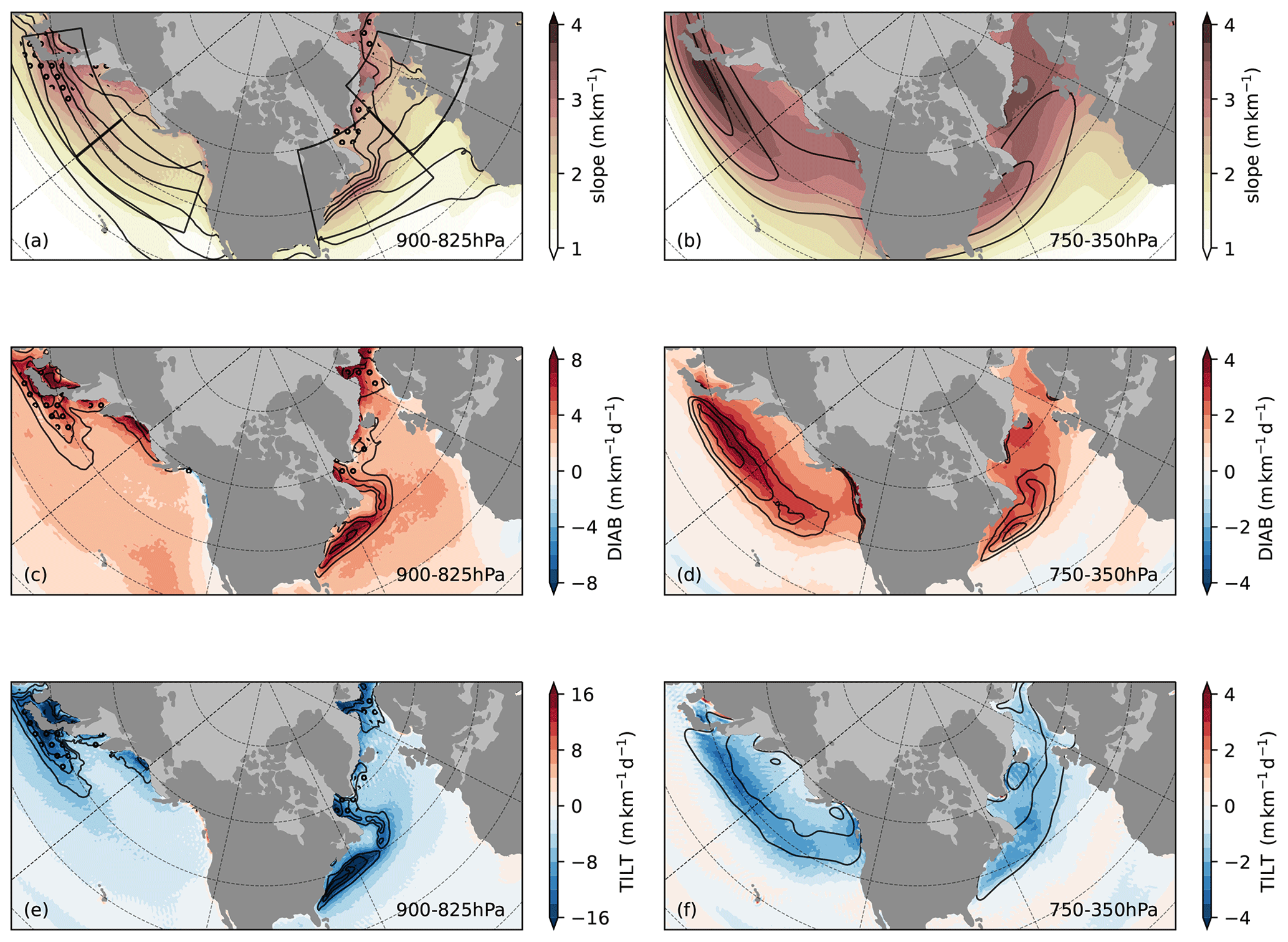
Figure 1 Winter (NDJF) climatology of (a, b) isentropic slope S, (c, d) DIAB, and (e, f) TILT (shading). Climatological means for the near-surface (900–825 hPa; a, c, e) and free troposphere (750–350 hPa; b, d, f). Solid contours represent (a) SST (every 4 ^∘C between 4 and 24 ^∘C), (b) wind speed at the dynamical tropopause (i.e. at 2PVU; 30, 40, 50 m s⁻¹), (c) surface heat flux (latent plus sensible, 50, 75, 100 W m⁻², positive upwards), (d) total precipitation (convective plus large scale; 5, 6, 7 mm d⁻¹), (e) CAO index (2, 3, 4 K), and (f) cyclone track densities (10, 20, 30 cyclones per season; Gaussian kernel of size 200 km used for estimation). Stippling represents areas where slope values are masked for between 25 % and 50 % of the time. Also marked in (a) are the regional domains chosen for spatial averaging.

Near the surface, the steepest climatological mean slope (2.5–3 m km⁻¹) is found along the strong gradients in SST associated with the oceanic western boundary currents (Fig. 1a). Temperature contrasts along the sea ice edge and low static stability within CAOs can also contribute to a steeper slope over the ocean basin (Papritz et al., 2015; Papritz and Spengler, 2017). Both DIAB and TILT reach their highest intensity in proximity to the SST gradients associated with the SST front found along western boundary currents (7–8 m km⁻¹ d⁻¹ for DIAB, 15–17 m km⁻¹ d⁻¹ for TILT). The same areas of strongest DIAB and TILT also coincide with strong surface heat fluxes (Fig. 1c) and a higher occurrence of CAOs (Fig. 1e).

In the free troposphere, the slope peaks along the main storm track regions in the Northern Hemisphere (2.5–3.25 m km⁻¹; Fig. 1b), while DIAB and TILT both feature maximum values along regions of steep slope (Fig. 1d and f, respectively, with absolute values of up to 3 m km⁻¹ d⁻¹), peaking slightly further downstream in both the North Atlantic and North Pacific basins. The slope peaks on the poleward flank of the climatological jet (Fig. 1b), while the most intense precipitation and highest storm track density appear to be tightly linked with the strongest DIAB and TILT (Fig. 1d, f).

4 Phase-space perspective on storm tracks

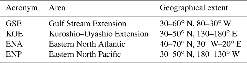
While the climatology is instructive on the mean structure of mid-latitude storm tracks (Fig. 1), it does not provide further insight into the temporal variability associated with the evolution of the two major storm tracks in the Northern Hemisphere. Hence, we consider spatial averages over four regions (see boxes in Fig. 1a) that are expected to behave similarly, both geographically and vertically. The four domains (Fig. 1a, Table 1) represent the upstream (Gulf Stream Extension, GSE; Kuroshio–Oyashio Extension, KOE) and downstream (Eastern North Atlantic, ENA; Eastern North Pacific, ENP) sectors of both the North Atlantic and North Pacific storm tracks. In the upstream regions, the slope features peak intensity in correspondence with strong SST gradients. Over the downstream regions, the slope is more evenly distributed spatially and maxima align with the most intense weather activity (as measured by storm track density; Fig. 1f).

Table 1 List of the regions used for spatial averaging.

4.1 Construction of time series

In spatially averaging over the respective domains (Table 1), we exclude land grid points to minimise the effect of orography on the slope diagnostics (Papritz and Spengler, 2015). We also exclude ocean surfaces with sea ice concentration above 15 % for more than 5 % of the time to limit the effects of inaccuracies in representing sea ice in reanalyses (Renfrew et al., 2021). Finally, we leave out any grid points pertaining to the Mediterranean and Baltic seas to avoid interference from local, mesoscale dynamics. We apply the same exclusion criteria for both the near-surface and free troposphere for the sake of consistency.

The time series of the slope, DIAB, and TILT for the 2013–2014 winter season are characterised by peaks of intense activity interspersed among periods of weaker-amplitude variability (Fig. 2). This sporadic nature in the temporal variability of the slope and its tendencies is primarily associated with the synoptic evolution that exerts a similar influence on meridional and surface heat fluxes (Messori and Czaja, 2013; Marcheggiani and Ambaum, 2020).

DIAB and TILT generally have opposite signs, both for the sample season and for the climatology. There are instances where they change sign, most often for TILT rather than DIAB. This is mainly due to orographic effects (e.g. gravity waves and other mesoscale features excited by mountain ranges) advected over the ocean that can result in significant positive TILT and thus dominate its domain-averaged value, especially when TILT is generally weak. The spatial domains were thus adjusted to reduce the impact of these undesired orographic effects.

While both DIAB and TILT appear to evolve almost instantaneously, a closer inspection of the time series reveals the existence of a phase shift between the two, hinting at the possibility that one leads in time over the other. The sum of DIAB and TILT tends to be positive (not shown), with positive (negative) values appearing to correspond to a higher (lower) slope. While the advection term is substantially weaker than DIAB and TILT (not shown), its magnitude is comparable to that of DIAB plus TILT, which suggests that part of the imbalance between DIAB and TILT is compensated for by advection. To better understand the observed relationship between DIAB and TILT, we utilise a phase-space analysis, which is particularly useful in studying the dynamical evolution of chaotic systems (Novak et al., 2017; Yano et al., 2020; Marcheggiani and Ambaum, 2020; Marcheggiani et al., 2022).

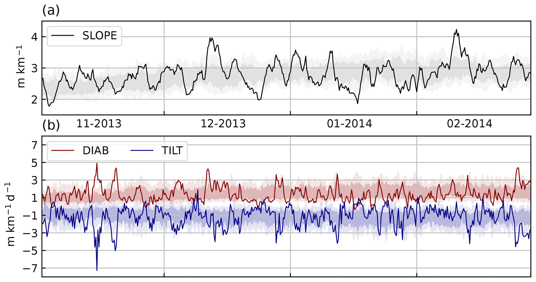
Figure 2 Time series of (a) free-tropospheric isentropic slope and (b) DIAB and TILT, spatially averaged over the GSE region. Solid lines represent a sample season (NDJF 2013–2014), while light (dark) shading represents the interdecile (interquartile) ranges over the climatological period (1979–2017).

4.2 Construction of phase portraits

We construct a phase space, where the x and y axes measure the average DIAB and TILT, respectively. We then plot the time series of DIAB against TILT, yielding trajectories in the phase space. Given the length of the time series and its irregular variability, we need to apply a kernel smoother to evince the typical phase-space circulation, where no time filtering was applied to the original time series. We use a Gaussian kernel to minimise the amount of noise without losing significant features of the phase-space circulation. Our results are qualitatively unchanged for different reasonable choices of the kernel size, and we refer the reader to Novak et al. (2017) and Marcheggiani et al. (2022) for more details on the applied kernel smoothing.

Once we obtained the average velocity field $\mathit{c}=(c_x,c_y)$ in the phase space, we define a streamfunction ψ to visualise the non-divergent flow F=αc, or mass flux, as α represents data density at each point in the phase space, such that

$$\begin{array}{}\text{(3)}& \mathit{F}=(\mathit{\alpha }{c}_x,\mathit{\alpha }{c}_y)=\left(-{\displaystyle \frac{\mathrm{d}\mathit{\psi }}{\mathrm{d}y}},{\displaystyle \frac{\mathrm{d}\mathit{\psi }}{\mathrm{d}x}}\right).\end{array}$$

We thus obtain a phase portrait of the DIAB–TILT co-evolution. If two variables are completely unrelated to each other, the corresponding phase portrait would be extremely noisy and incoherent, regardless of filter strength and/or size, while for two variables that are directly proportional to each other the circulation would collapse onto a diagonal. Departures from the diagonal are indicative of the existence of a phase shift in their co-evolution, whereby one leads in time. In the extreme case of a 90^∘ phase shift, the resulting phase portrait would feature a perfectly circular circulation. One can also estimate the mean value of any variable across the phase space by calculating its kernel average, where we consider the area-mean slope and calculate its kernel average to inspect its variability in parallel to the evolution of DIAB and TILT (Fig. 3).

Inspecting phase portraits for each pressure level individually (not shown), we found a reversal in the phase-space mean circulation between 825 and 750 hPa, transitioning from anticlockwise in the near-surface (Fig. 3e–h) to clockwise in the free troposphere (Fig. 3a–d). We accommodate for this dichotomy by separating our analysis into the near-surface (900–825 hPa) and the free troposphere (750–350 hPa). Although previous studies already adopted a similar vertical separation (e.g. Papritz and Spengler, 2015, used 600 hPa as partition level), our phase-space analysis allows for a more dynamically motivated separation of levels. The circulation changes structure entirely as we reach levels above 350 hPa (not shown), where stratospheric dynamics most likely become more relevant and affect the typical circulation.

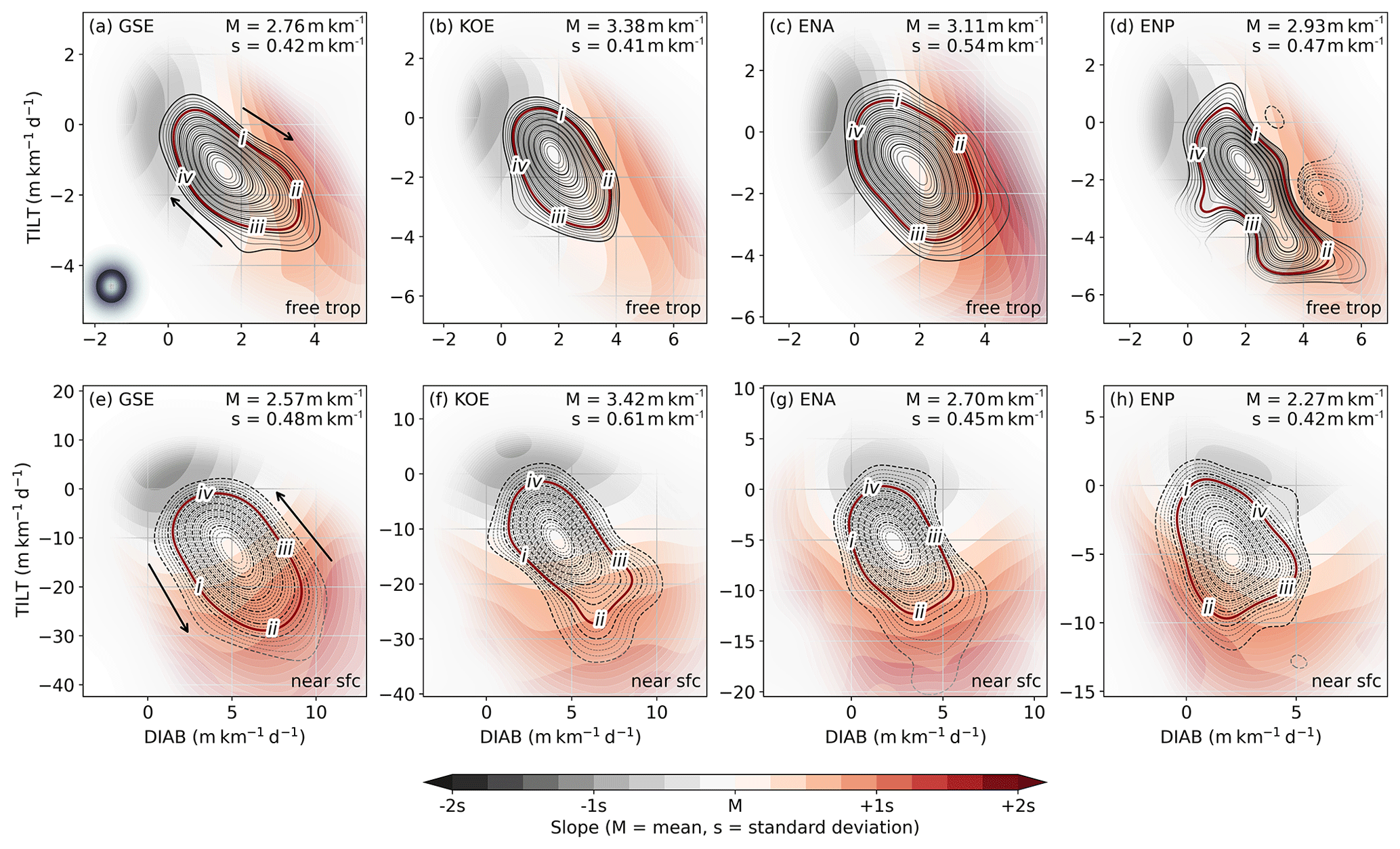
Figure 3 Phase portraits of spatially averaged DIAB (x coordinate) and TILT (y coordinate). Shading represents the kernel-averaged mean-slope: offset and scale are according to the mean and standard deviations of the slope time series, respectively, which are annotated in the upper-right corner of each panel. Contours represent the stream functions associated with the kernel-averaged phase-space circulation, with positive (solid) and negative (dashed) values indicating a clockwise and anticlockwise direction, respectively. Arrows in panels (a) and (e) indicate explicitly the direction of the circulation. Grid points are faded according to data density, so kernel averages for points where data are scarce are blanked out. The upper panels show phase portraits for the free-tropospheric GSE (a), KOE (b), ENA (c), and ENP (d) regions, while the corresponding panels below show phase portraits for the near-surface. The size of the Gaussian filter used to construct the phase portraits is indicated by the shaded black dot in the lower-left corner of panel (a), while the white dot within it represents that for the computation of kernel composites in Figs. 5–10. Roman numerals (i, ii, iii, iv) indicate the four different points in the phase space where the kernel composites are evaluated (see Figs. 5–10).

4.3 Phase portraits

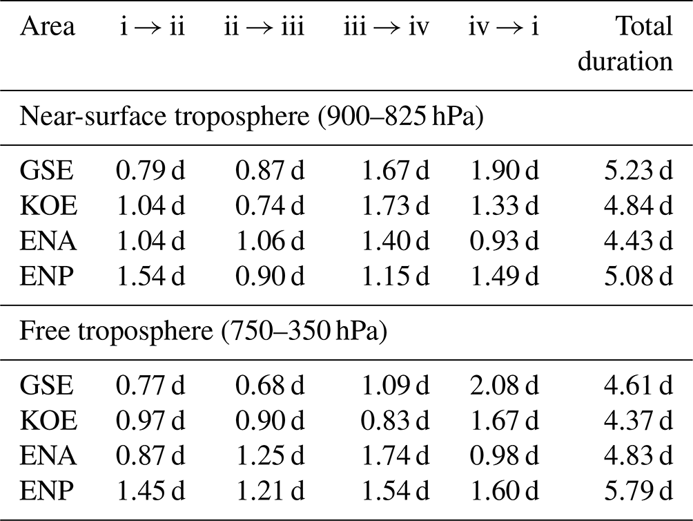
For all domains and vertical sections, there is a strong link between DIAB and TILT, as evinced by the near-diagonal alignment of the average circulation. As indicated, the main difference between the near-surface and free troposphere is the direction of the mean circulation in the phase space, with TILT leading DIAB in the near-surface troposphere and DIAB leading TILT in the free troposphere. We estimate the average duration for one revolution by integrating the phase speed (i.e. $\sqrt{{c_x}^{\mathrm{2}}+{c_y}^{\mathrm{2}}}$) along isolines of the streamfunction. For the closed trajectories shown in Fig. 3, we obtain values of about 5d, ranging between 4.3–5.8 d (see Table 2).

Table 2 Time periods between consecutive stages (i, ii, iii, and iv) as indicated in the phase portraits shown in Fig. 3 for each of the spatial domains (see Table 1) for the near-surface and free troposphere. The last column on the right shows the total duration along closed trajectories highlighted in Fig. 3.

Consistent with the climatology (Fig. 1), the magnitudes of both DIAB and TILT are largest near the surface, in particular over the upstream regions, with average values up to 30 m km⁻¹ d⁻¹ where the SST gradients are strongest (Fig. 3e, f), almost double the range of variability downstream (Fig. 3g, h). In the free troposphere, however, there is no substantial difference in the magnitude of the average tendencies between upstream and downstream regions (Fig. 3a–d).

The mean isentropic slope in the near-surface troposphere over the GSE region increases with the magnitude of both DIAB and TILT, reaching maximum values around 1 standard deviation above its time mean in the lower-right quadrant of the phase space (Fig. 3e), while it increases primarily with the magnitude of TILT and peaks in the lower half in the other regions (Fig. 3f–h).

Given that the net effect of TILT on the slope is negative, it might at first appear counter-intuitive that the near-surface slope increases with the magnitude of TILT. One possible explanation for this apparent contradiction is that the steepening of mean slope actively contributes to the strengthening of both TILT and DIAB. Using phase-space composites, we shed light onto the physical mechanisms behind the phase-space circulation (see Sect. 5).

In the free troposphere, on the other hand, DIAB leads TILT, and the area-mean slope increases primarily with DIAB in all of the domains considered (Fig. 3a–d). The interpretation is thus more straightforward, as the increase in slope with DIAB underlines the primary role of DIAB in generating enough slope for the development of baroclinic instabilities, which in turn is associated with an increase in TILT.

5 Phase-space composites

We can gather further insight into the mechanisms driving the phase-space circulation by evaluating composites of the atmospheric flow at various locations in the phase space. Specifically, we identify four stages corresponding to (i) increasing slope, (ii) steepest slope, (iii) decreasing slope, and (iv) weakest slope. The specific location of each stage within the phase space is shown in Fig. 3, and the inter-stage time intervals are indicated in Table 2. We determined the exact location of each stage to facilitate the comparison across the four spatial domains. Consequently, time intervals between different stages are somewhat different, ranging between ≈0.7–2 d. While the overall cycle duration is indicative of the timescale associated with a dynamical system, the duration of individual events may be shorter or longer.

We construct kernel composites of geopotential height at 1000 (Z1000) and 500 hPa (Z500), as the spatial shift between these two levels is informative on the baroclinic structure of the atmospheric flow, where we removed the winter climatology (Fig. 4) to highlight transient variability. Even in the climatology, the mid-latitude circulation features baroclinic growth with a westward tilt with height, as minima in Z1000 are located east of Z500 minima (Fig. 4).

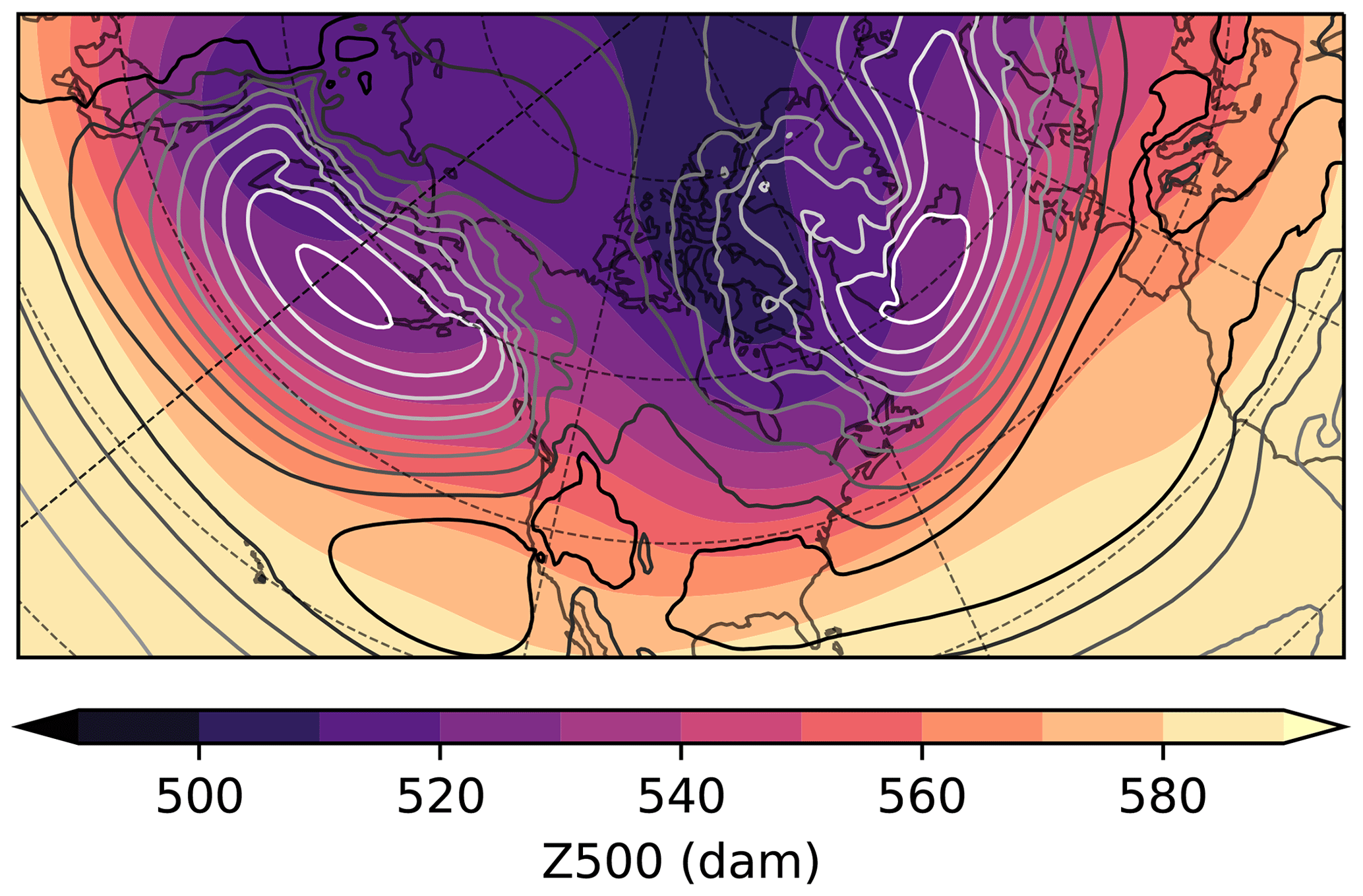
Figure 4 Winter climatology (NDJF, 1979–2017) of geopotential height at 500 hPa (Z500, shading) and 1000 hPa (Z1000, contours, every 2 dam between 0–15 dam, with whiter contours for lower geopotential).

We calculate composites of DIAB and TILT to visualise their spatial structure along a lifecycle, where we inspect full fields as opposed to anomalous fields, as the interpretation of anomalies for accumulated fields can be misleading. For the free troposphere, we also consider the full composites of TCWV and total precipitation (sum of large scale and convective) to highlight the connection between high levels of moisture availability and the bulk of diabatic processes associated with latent heating.

5.1 Near-surface composites

In the first stage, which is characterised by the intensification of TILT (see phase portraits, Fig. 3e–h), all of the four domains feature negative anomalies in Z500 and Z1000 (Fig. 5a, b and Fig. 6a, b), indicating advection of cold air from continents for KOE and GSE and from polar oceans over warmer ocean surfaces for ENP and ENA. The structure of the flow is consistent with the onset of CAOs, which are most frequent in these regions in winter (Grønås and Kvamstø, 1995; Dorman et al., 2004; Kolstad et al., 2009). The spatial distribution of strong TILT trails behind the advancing cold air front, while DIAB intensifies upstream of peaks in TILT (i.e. to their west). Strong DIAB and TILT outside of the averaging domain, such as over the Davis Strait for GSE composites or south of the Bering Strait for KOE composites (Fig. 5), likely reflect their climatological mean rather than a specific relevance to a particular stage in the phase portrait.

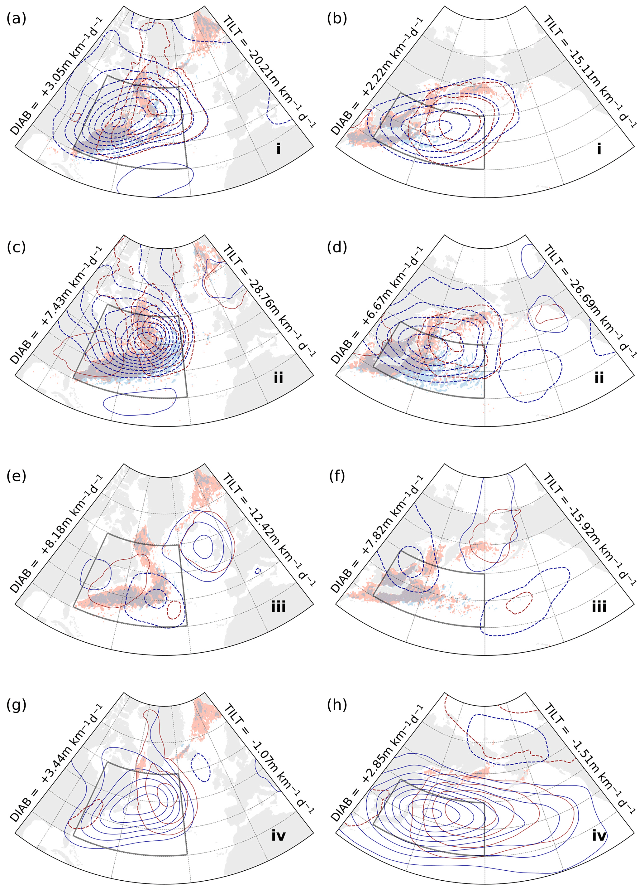
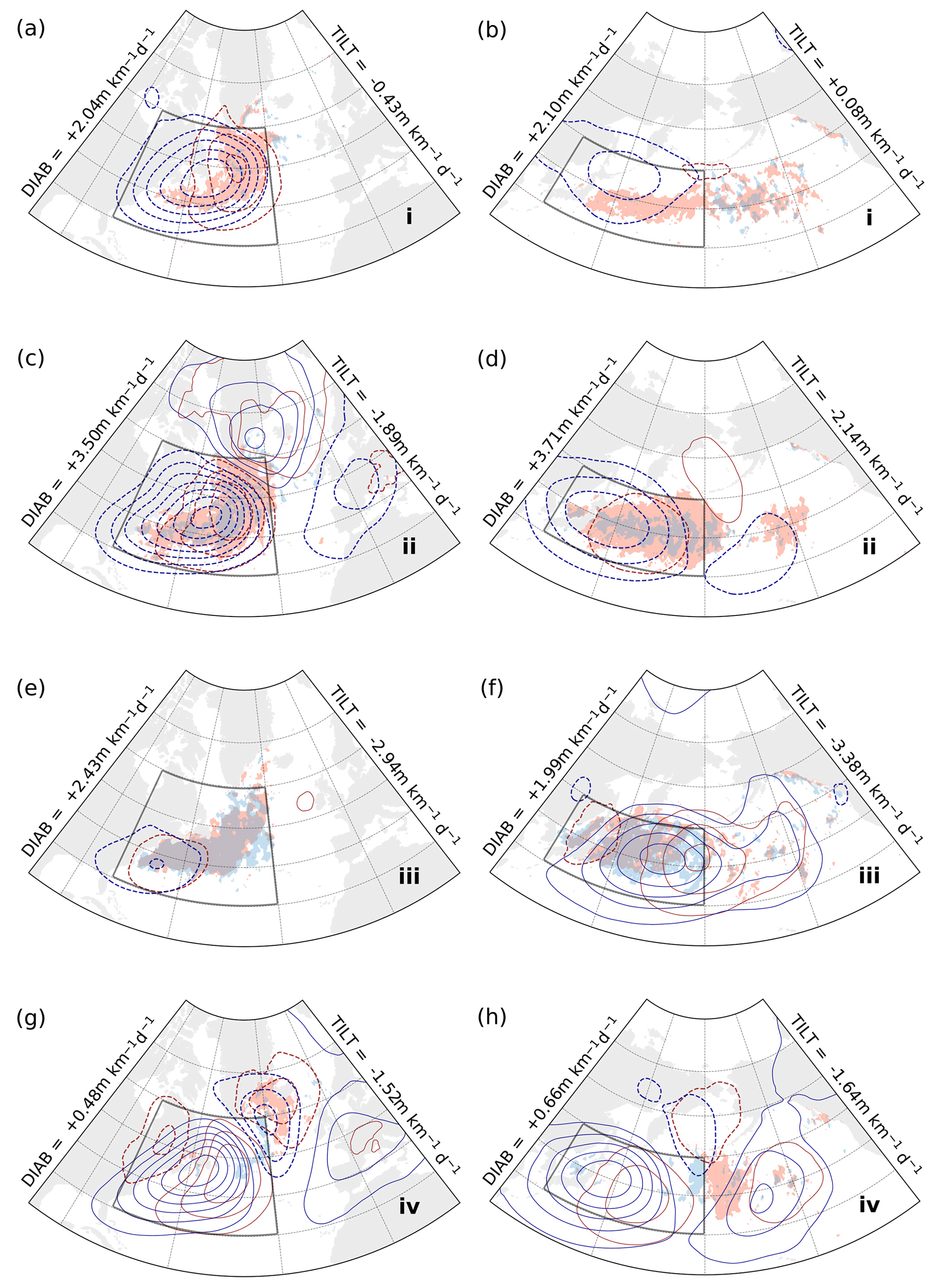
Figure 5 Kernel-averaged composites of Z1000, Z500, DIAB, and TILT for phases (a, b) i, (c, d) ii, (e, f) iii, and (g, h) iv in the phase portraits for the near-surface troposphere upstream regions GSE (left; Fig. 3a) and KOE (right; Fig. 3b). Contours of Z1000 and Z500 (red and blue, respectively) represent the anomaly field relative to climatology (NDJF, 1979–2017) and are plotted every 2 dam (0 dam contours omitted, negative contours dashed). Shading for DIAB (red) and TILT (blue) represents full composite (not anomalies) and indicates values above 15 m km⁻¹ d⁻¹ for DIAB and below −15 m km⁻¹ d⁻¹ for TILT. DIAB and TILT mean values are annotated for each stage on the sides of each map.

Figure 6 Same as in Fig. 5 but for the near-surface troposphere downstream regions ENA (left; Fig. 3g) and ENP (right; Fig. 3h). Shading for DIAB (red) and TILT (blue) indicates values above 6 m km⁻¹ d⁻¹.

According to phase portraits, the second stage is characterised by the steepest slope, as TILT reaches its maximum intensity while DIAB is still increasing. Composites for this stage (Fig. 5c, d; Fig. 6c, d) show a strengthening and, especially in the ENA region (Fig. 6c), a downstream progression of the cyclonic circulation that emerged in the previous stage. We observe again that the spatial distribution of TILT features a shift to the east with respect to that of DIAB, which is now dominant and gradually spreads westwards. For ENA and ENP (Fig. 6c, d), the westward tilt in geopotential becomes weaker compared to GSE and KOE (Fig. 5c, d), suggesting that the cyclonic anomalies downstream are in a more mature, barotropic stage. The associated atmospheric flow is, however, still favourable for CAOs, with northwesterly flow from the continents and northerly flow from the polar oceans.

In the third stage, TILT has subsided compared to the previous stage, while DIAB has retained its strength along the western boundary currents (Fig. 5e, f) or becomes even larger over the downstream regions (Fig. 6e, f). The picture is somewhat different for the ENP region, where TILT does not appear to have changed much, while DIAB is visibly stronger. CAOs are no longer active within the domains, as the cyclonic circulation gradually weakens and positive anticyclonic geopotential anomalies start building up in the western part of the domains, except for the KOE region, where positive anomalies have not yet formed at this stage.

The anticyclonic circulation emerging in the third stage becomes a dominant feature of the fourth and final stage, where TILT and DIAB as well as the mean slope are weakest (Fig. 5g, h; Fig. 6g, h). These anticyclonic anomalies mainly represent the anomalously low cyclonic activity, which is consistent with the weaker mean slope observed in the phase portraits (Fig. 3e–h). The vertical structure is still baroclinic in the upstream regions (Fig. 5g, h), while it is more barotropic downstream (Fig. 6g, h), reflecting the climatological structure of the atmospheric flow in these regions.

In the near-surface, we can therefore ascribe the particular phasing between DIAB and TILT to the effect of cold air advection associated with CAOs and cold sectors of mid-latitude weather systems. The propagation of the cold front associated with these events contributes to a local steepening of the slope. Steep slope prompts an almost instantaneous response in TILT, whereby isentropic surfaces are flattened as cold air masses sweep in over the ocean surface. The thermal contrast between the cold air masses and the warm ocean surface eventually triggers surface heat fluxes which act to anchor the isentropic surfaces back to their initial position, thus diabatically restoring the near-surface slope.

5.2 Free-troposphere composites

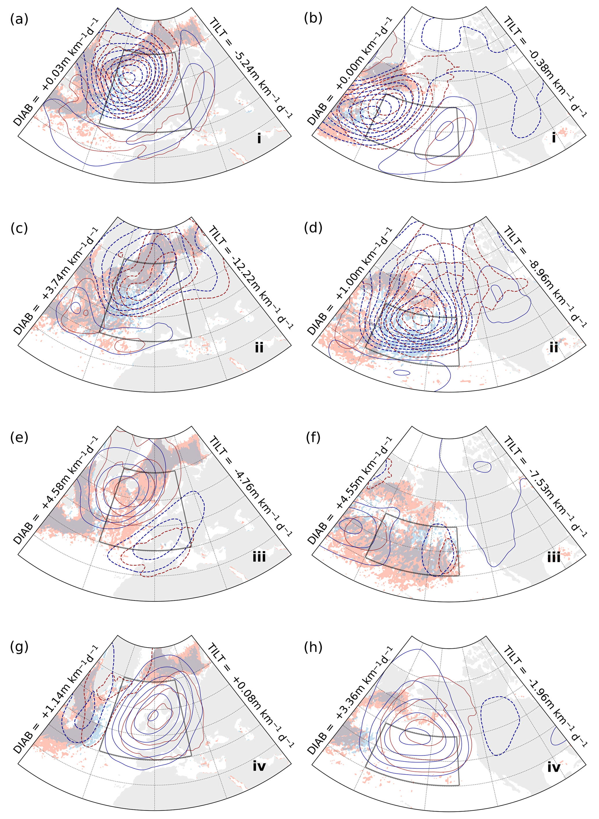
In the phase portraits for the free troposphere, the slope concurs to a greater degree with changes in DIAB rather than changes in TILT. In the first stage, slope is slowly building up and composites show cyclonic geopotential height anomalies forming either within (GSE and KOE, Fig. 7a and b, respectively) or slightly to the west of the spatial domain (ENA and ENP, Fig. 8a and b, respectively). DIAB is most active in close proximity to these cyclonic anomalies, particularly on the southern and western flanks of the upper-level anomalies, with the exception of the ENA region (Fig. 8a), where DIAB is somewhat weaker overall and peaks to the north of the upper-level anomaly. TILT, on the other hand, remains negligible across the four regions.

Figure 7 Same as in Fig. 5 but for the free-troposphere upstream regions GSE (left; Fig. 3a) and KOE (right; Fig. 3b). Shading for DIAB (red) and TILT (blue) indicates values above 3 m km⁻¹ d⁻¹ for DIAB and below −3 m km⁻¹ d⁻¹ for TILT.

The cyclonic anomalies deepen further in the second stage, especially in the GSE (Fig. 7c), ENA (Fig. 8c), and ENP (Fig. 8d) regions, while a similar but weaker development is evident in KOE (Fig. 7d). Positive anticyclonic anomalies are also forming to the east of the cyclonic anomalies, while a second negative anomaly develops further eastward in the ENP composite (Fig. 8d). The area of most intense DIAB broadens substantially, almost spanning the entire domains in KOE and ENP (Figs. 7d and 8d), while TILT also strengthens in correspondence to the cyclonic anomalies and within areas of intense DIAB.

Figure 8 Same as in Fig. 5 but for the free-troposphere downstream regions ENA (left; Fig. 3c) and ENP (right; Fig. 3d). Shading for DIAB (red) and TILT (blue) indicates values above 3 m km⁻¹ d⁻¹ for DIAB and below −3 m km⁻¹ d⁻¹ for TILT.

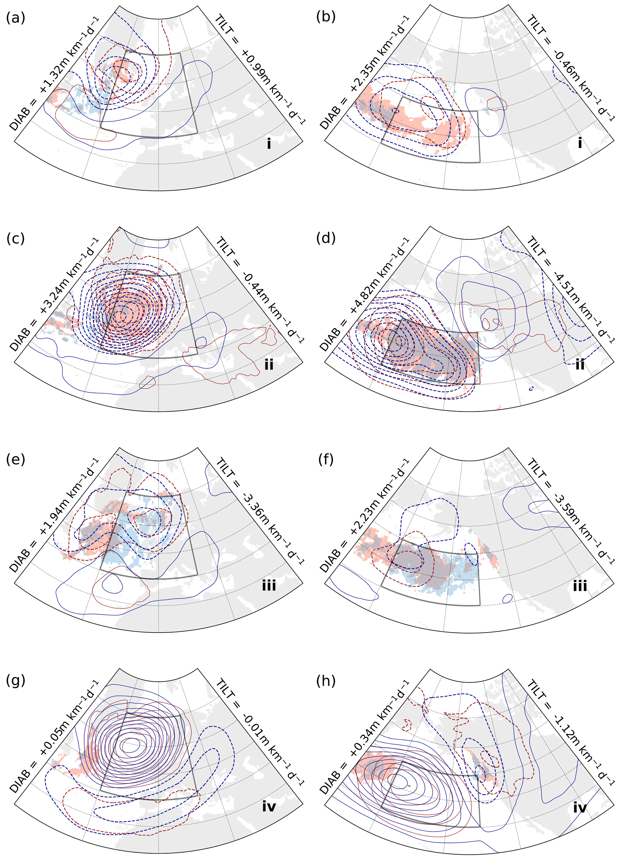
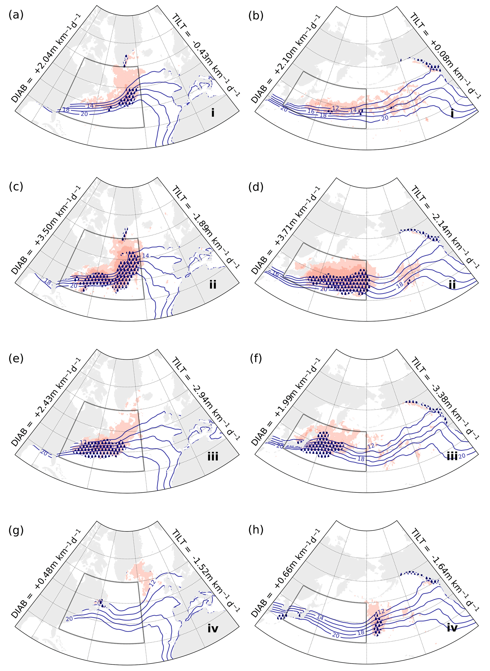
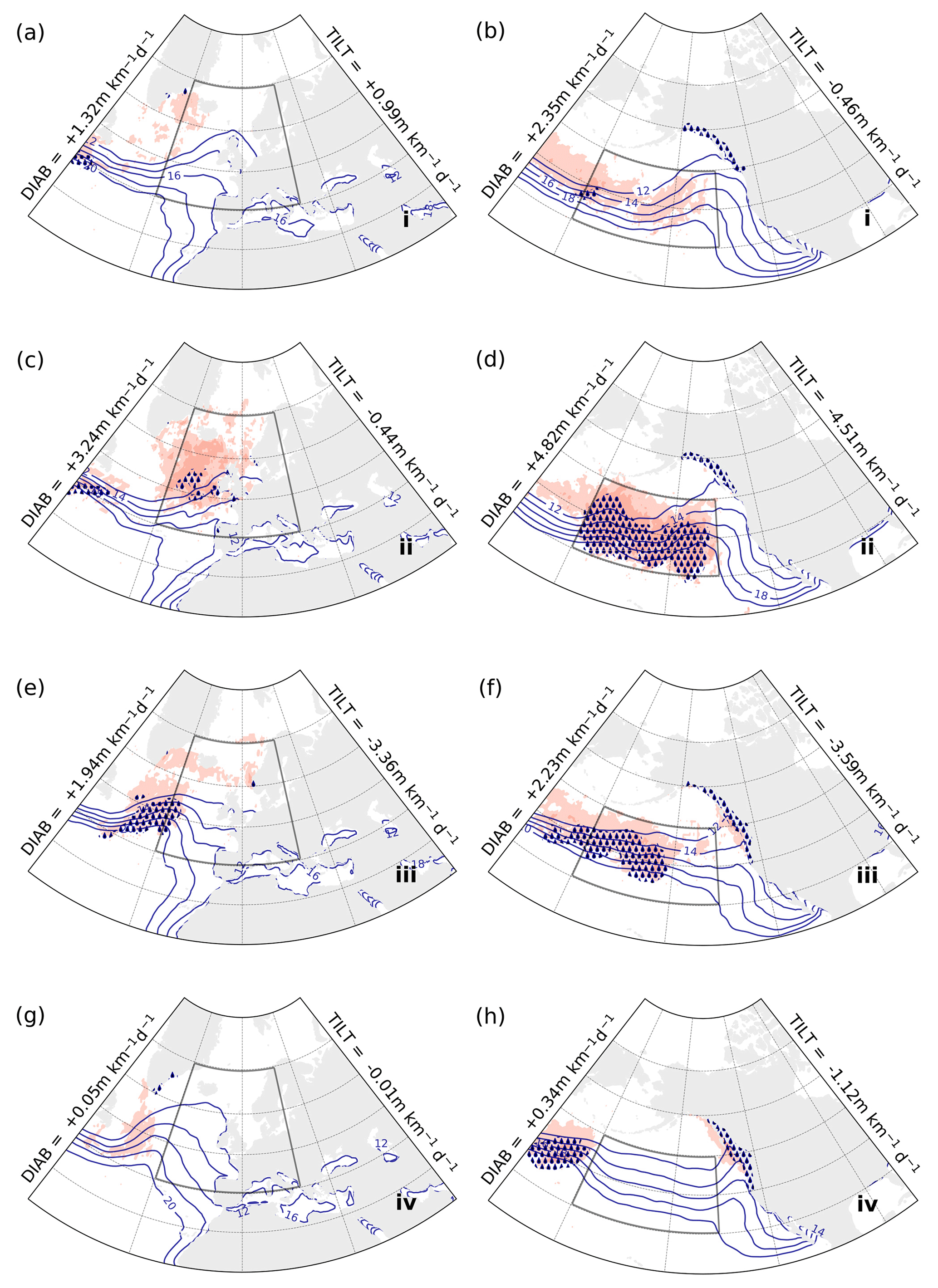
Figure 9 Kernel-averaged composites of DIAB (red shading, lighter above 3 m km⁻¹ d⁻¹, darker above 5 m km⁻¹ d⁻¹), TCWV (blue contours, every 2 kg m⁻² between 12–20 kg m⁻²), and total precipitation (stippling, above 8 mm d⁻¹) for phases i (a, b), ii (c, d), iii (e, f), and iv (g, h) in the phase portraits for the free-troposphere upstream regions GSE (left; Fig. 3a) and KOE (right; Fig. 3b).

Figure 10 Same as in Fig. 9 but here for the free-troposphere downstream regions ENA (left; Fig. 3c) and ENP (right; Fig. 3d).

The third stage is characterised by a breakdown of the cyclone–anticyclone system. The amplitude of the geopotential height anomalies is visibly reduced in the composites for GSE, ENA, and ENP (Figs. 7e; 8e, f), while their vertical structure becomes more barotropic, especially in ENA and ENP. The evolution in the KOE (Fig. 7f) is somewhat distinct from that for the other regions, as anticyclonic anomalies, still with a baroclinic structure, become dominant across the domain, while the cyclonic anomalies from the previous stage are waning to their west. In all four domains, however, we observe DIAB subsiding, while TILT remains relatively strong. Phase portraits indicate that mean slope is also decreasing, which, coupled with a stronger TILT, is expected to hinder further synoptic development.

In the fourth stage, mean slope is close to its minimum value and composites reveal positive geopotential anomalies dominating the four spatial domains (Fig. 7g, h; Fig. 8g, h). Both DIAB and TILT are weak, with the only visible traces outside the domains and mostly linked to their climatological distribution (Fig. 1d, f).

Both the steepest slope and highest DIAB occur in the second stage when the cyclonic activity that developed in the first stage reaches its maximum intensity. The geopotential anomaly pattern resembles a propagating Rossby wave stretching across the ocean basins, which is most evident for GSE (Fig. 7c) and ENP (Fig. 8d) and to a lesser extent for KOE (Fig. 7d) and ENA (Fig. 8c). In all composites, Z1000 and Z500 anomalies at stages (ii) and (iv) share a similar spatial pattern but with opposite signs, while stages (i) and (iii) reflect the transition between opposing phases of the Rossby wave packet. Inspecting composites at intermediate stages (not shown), we are able to reconstruct the propagation of a Rossby wave across the North Atlantic and Pacific oceans, and the specific phasing between DIAB and TILT, with DIAB leading TILT, appears essential in its propagation.

Recent studies have shown that precipitation in climate models can have a significant impact on the representation of storm tracks and jet variability (Schemm, 2023; Fuchs et al., 2023). However, the mechanisms that explain these sensitivities in modelled storm track variability remain unclear. As latent heating associated with precipitation constitutes the bulk of diabatic processes in the free troposphere (Papritz and Spengler, 2015), we can gather further insight into the role of moisture in storm track dynamics by looking into the evolution of TCWV and total precipitation in the TILT–DIAB phase space.

Across all four regions, the most intense precipitation occurs during the second stage (panels c and d in Figs. 9–10) and, to a lesser extent, during the third stage (panels e and f in the same figures). Although differences in the distribution of TCWV from one stage to the other can be subtle, they are consistent with composites of total precipitation and DIAB. In particular, we find spatial correspondence between maxima in precipitation and strongest DIAB (darker shading in Figs. 9–10), which is consistent with the primary importance of latent heat release in the diabatic restoration of slope (Papritz and Spengler, 2015).

Most of the precipitation appears to be located along trailing cold fronts associated with the strongest cyclonic anomalies (panels c–f in Figs. 9–10), while much weaker signals emerge during stages dominated by anticyclonic anomalies (panels a, b, g, and h in Figs. 9–10). There is a reduction in TCWV behind the cold front, which is linked to the relatively dry air mass associated with the cold sector. Some of the precipitation is also found to the east of the cyclonic systems (most clearly for GSE, KOE, and ENP), in correspondence with their warm sectors where TCWV is larger.

The close relationship that we found between DIAB, precipitation, and TCWV is consistent with the hypothesis that moisture availability plays a crucial role in the evolution of cyclones and is most likely linked to pulses in storm track activity, as suggested by Weijenborg and Spengler (2020). However, sensitivity experiments are needed to validate this hypothesis.

6 Conclusions

We find that adiabatic (TILT) and diabatic (DIAB) changes in the slope of isentropic surfaces are strongly tied to each other throughout the troposphere, both in space (Fig. 1) and time (Fig. 2). Conducting a phase-space analysis, we reveal a phasing between DIAB and TILT, which is of opposite sign in the near-surface (900–825 hPa) and free troposphere (750–350 hPa) (Fig. 3), where TILT and DIAB lead, respectively.

In the near-surface troposphere, TILT leads DIAB (Fig. 3e–f). Composite analysis suggests that this phasing between TILT and DIAB is associated with the advection of cold air masses during CAOs over the warmer ocean. The advection of cold air masses onto the ocean surface yields an initial flattening of isentropic surfaces, almost instantaneously followed by a response in surface heat fluxes upstream that restores the slope (Figs. 5, 6).

We notice that the increase in mean slope occurs when TILT is stronger than DIAB, while the steepest slope is found when the magnitudes of both TILT and DIAB are largest. This might seem counter-intuitive, as strong TILT would be expected to lead to a reduction in slope. However, we can understand this if we reframe the causal link between slope and its tendencies. In the presence of an anomalously steep slope, a strong TILT would ensue to reduce it. As cold fronts associated with cold air masses bring anomalously steep slopes into the spatial domain, the mean slope increases. The steep slope triggers an immediate response in TILT. While TILT continues downstream, upstream surface heat fluxes gradually anchor isentropic surfaces back to the ocean surface temperature gradient, which results in the diabatic restoration of slope measured by DIAB. Thus, changes in the near-surface slope actually condition DIAB and TILT, explaining the circulation in the phase space.

In the free troposphere, on the other hand, phase portraits point to the primary role of DIAB for the phase-space circulation, as DIAB leads in time over TILT, while their intensification goes hand in hand with the steepening of the slope (Fig. 3a–d). Composites across the phase space confirm that DIAB is tightly linked to the development and further evolution of storm activity, both in time and space (Figs. 7, 8). In particular, the evolution of the anomalous circulation (Z1000 and Z500) across the different stages identified in the phase portraits is reminiscent of a Rossby wave packet propagating over the North Atlantic and Pacific Ocean basins. As composites are based exclusively on changes in DIAB and TILT, the specific phasing between DIAB and TILT appears thus an essential feature of these Rossby wave packets.

Furthermore, we find that most of DIAB coincides with peaks in precipitation and overall moisture availability (Figs. 9, 10), further underlining the differences that sensible and latent heating play in the lower and upper troposphere, respectively, as pointed out in previous studies (e.g.  Hoskins and Valdes, 1990; Hotta and Nakamura, 2011; Papritz and Spengler, 2015). The close link between free-tropospheric DIAB and moisture availability adds to a growing body of literature highlighting the importance of moist diabatic processes and their correct representation in numerical models to reduce model biases in storm track location and intensity (Willison et al., 2013; Schemm, 2023; Fuchs et al., 2023), pinpointing the need to develop a more comprehensive moist storm track model. Sensitivity experiments would be needed, however, to further validate the causal link between moisture availability and diabatic generation of slope.