the Creative Commons Attribution 4.0 License.
the Creative Commons Attribution 4.0 License.
 | 04 Mar 2024
Sustained intensification of the Aleutian Low induces weak tropical Pacific sea surface warming
Christine M. McKenna
Manoj M. Joshi
Adam T. Blaker
Richard Rigby
Amanda C. Maycock
It has been proposed that externally forced trends in the Aleutian Low can induce a basin-wide Pacific sea surface temperature (SST) response that projects onto the pattern of the Pacific Decadal Oscillation (PDO). To investigate this hypothesis, we apply local atmospheric nudging in an intermediate-complexity climate model to isolate the effects of an intensified winter Aleutian Low sustained over several decades. An intensification of the Aleutian Low produces a basin-wide SST response with a similar pattern to the model's internally generated PDO. The amplitude of the SST response in the North Pacific is comparable to the PDO, but in the tropics and southern subtropics the anomalies induced by the imposed Aleutian Low anomaly are a factor of 3 weaker than for the internally generated PDO. The tropical Pacific warming peaks in boreal spring, though anomalies persist year-round. A heat budget analysis shows the northern subtropical Pacific SST response is predominantly driven by anomalous surface turbulent heat fluxes in boreal winter, while in the equatorial Pacific the response is mainly due to meridional heat advection in boreal spring. The propagation of anomalies from the extratropics to the tropics can be explained by the seasonal footprinting mechanism, involving the wind–evaporation–SST feedback. The results show that low-frequency variability and trends in the Aleutian Low could contribute to basin-wide anomalous Pacific SST, but the magnitude of the effect in the tropical Pacific, even for the extreme Aleutian Low forcing applied here, is small. Therefore, external forcing of the Aleutian Low is unlikely to account for observed decadal SST trends in the tropical Pacific in the late 20th and early 21st centuries.
- Article
(7228 KB) - Full-text XML
-
Supplement
(2558 KB) - BibTeX
- EndNote


The Aleutian Low has a well-known role in determining the North Pacific component of the Pacific Decadal Oscillation (PDO) (e.g. Schneider and Cornuelle, 2005; Zhang et al., 2018; Hu and Guan, 2018; Sun and Wang, 2006; Newman et al., 2016). Fluctuations in Aleutian Low intensity affect the North Pacific subpolar gyre (Pickart et al., 2009), upper ocean temperatures (e.g. Latif and Barnett, 1996), and sea surface height (Nagano and Wakita, 2019) through anomalous thermal forcing and wind stress. Oceanic Rossby waves initiated by Aleutian Low variability can propagate westward and cause lagged signals in the Kuroshio–Oyashio extension (KOE) region (e.g. Kwon and Deser, 2007).
The traditional paradigm for the PDO describes the integrated effect of mid-latitude stochastic variability, which induces sea surface temperature (SST) anomalies through turbulent heat flux and wind stress curl anomalies, and driving from tropical processes (El Niño–Southern Oscillation, ENSO, variability) via excitation of Rossby wave trains and tropical–extratropical teleconnections (Newman et al., 2016; Zhao et al., 2021; Vimont, 2005; Knutson and Manabe, 1998; Jin, 2001). We note that recent definitions separate low-frequency PDO variability and show this is predominantly associated with stochastic extratropical atmospheric variability (i.e. the Aleutian Low) (Wills et al., 2019). However, decadal changes in the Aleutian Low may arise via other mechanisms including Arctic sea ice trends (Simon et al., 2021; Deser et al., 2016), stratospheric polar vortex variability (Richter et al., 2015), or as a local response to external forcings (Smith et al., 2016; Dow et al., 2021; Dittus et al., 2021). It has been proposed that observed shifts in the PDO in the late 20th and early 21st centuries were driven by anthropogenic forcing of the Aleutian Low, which was then communicated to a basin-wide PDO signal (Smith et al., 2016; Gan et al., 2017). However, the mechanisms by which North Pacific anomalies linked to decadal Aleutian Low changes may be communicated into a basin-wide SST response including the tropics, and whether the amplitude of such a response matches observed variations, remain unclear.
In this study, we aim to better understand the role of long-term changes in the Aleutian Low in governing the multi-annual behaviour of tropical Pacific SSTs. We perform an ensemble of atmospheric nudging simulations in an intermediate-complexity coupled climate model to isolate the effect of a sustained anomaly in the Aleutian Low. The response to this regional perturbation is compared to the internally generated low-frequency Pacific variability in a free running simulation. The article is structured as follows: Sect. 2 describes the methodology and details of the model used. Section 3 compares the results of the nudging simulations with the free running simulation. Discussion of the results is provided in Sect. 4 and conclusions in Sect. 5.
2.1 FORTE2.0
Simulations were performed using FORTE2.0, an intermediate-complexity coupled atmosphere–ocean general circulation model (AOGCM) (Blaker et al., 2021). The atmospheric model IGCM4 (Intermediate General Circulation Model 4) (Joshi et al., 2015) uses a truncated series of spherical harmonics run at T42 resolution with 20 Σ levels to a height of Σ= 0.05. IGCM4 is coupled to the MOMA (Modular Ocean Model – Array) (Webb, 1996) ocean model run at 2° × 2° resolution with 15 vertical levels. The two components are coupled once per day using OASIS version 2.3 (Terray et al., 1999) and PVM version 3.4.6 (Parallel Virtual Machine). As described in Blaker et al. (2021), between 5° N/S and the Equator the horizontal ocean diffusion increases by a factor of 20 to balance equatorial upwelling and parameterise the eddy heat convergence. For more details on the model see Blaker et al. (2021). The model simulates multi-decadal SST variability in the Pacific with a similar pattern to that seen in observations but a weaker amplitude by around a factor of 4 to 5 (Fig. S1 in the Supplement). While the model is run at relatively low horizontal and vertical resolution, the model code is sufficiently flexible to apply the nudging method described in Sect. 2.2, and the model is computationally efficient to run, enabling a large ensemble to be produced.
2.2 Grid-point nudging method
Atmospheric nudging has been used to investigate climate and weather relationships between remote phenomena (e.g. Martin et al., 2021; Knight et al., 2017; Watson et al., 2016). A nudging code was added to IGCM4. Nudging was performed by adding tendencies to horizontal winds, temperature, and surface pressure. The nudging code is publicly available at (https://github.com/NOC-MSM/FORTE2.0, last access: 13 August 2023).
The nudging configuration is similar to that in Watson et al. (2016), with two additional terms to account for vertical (z) and temporal (t) variation in the nudging strength:
where x is the variable being relaxed as a function of longitude (λ) and latitude (ϕ), xref is the reference state, and τ is the nudging strength (set to 6 h). The spatial extent of the nudging was tested extensively to avoid any shock at the boundaries and spurious effects of nudging near polar regions. The regional extent was determined as
where
and
Φ1= 30° N and Φ2= 65° N represent the southern and northern nodal points of the nudging region, and λ1= 160° E and λ2= 140° W are the eastern and western nodal points of the nudging region. The coefficients δ1= 0.05, δ2= 1, and δ3= 0.2. The horizontal limits follow the commonly defined North Pacific Index (NPI) (Trenberth and Hurrell, 1994) as a proxy for the region encompassed by the Aleutian Low. Within the nudging patch shown in Fig. S2, the values are scaled so that the maximum value equals 1.
The temporal and nudging variations are determined as
The strength of the tropospheric nudging is set to 1 (constant a, Eq. 5) at z= 0.96 (lowest atmospheric level), decreasing exponentially to 0 at z= 0.05 (tropopause) (Eq. 5). Nudging is applied during the extended boreal winter season (NDJFM) peaking on 15 January, with a Gaussian function in time to increase the nudging strength from 0 to 1 between 1 and 30 November and a reverse ramp-down during March. Term d (Eq. 6) is the time difference relative to maximum nudging time in months (e.g. d=0 on 15 December, d= −1 on 15 January), β is a constant set to 1.2, and µ is a constant set to 2. Outside of the nudging window, h=0. The spatio-temporal forms of the nudging coefficients are shown in Fig. S2.
The strong Aleutian Low state is taken from a 100-year-long control run based on a winter month with an NPI anomaly of −10.76 hPa, or −3.02σ, where σ = 3.53 hPa is the standard deviation calculated over all winter months in the control (Fig. S3). Therefore, the target state represents an extreme intense Aleutian Low state as simulated in FORTE2.0. Compared with ERA5 reanalysis data from 1979–2020, a 1σ NPI anomaly is 5.20 hPa. The imposed atmospheric forcing is therefore weaker than if an equivalent experiment were conducted using a comparably sized NPI anomaly in reanalysis data. A 50-member nudged ensemble was generated using initial conditions drawn from each 1 January of the final 50 years of control. Each member is integrated for 30 years with nudging commencing on 1 November of the first year and repeating each winter of the simulation. Unless otherwise stated, the analysis shows ensemble mean anomalies in the nudged simulation compared to the long-term climatology of control. Statistical significance of the ensemble mean difference is estimated as being where the anomaly ±2 standard error does not overlap zero. Standard error (SE) is calculated as
where σ is the inter-ensemble standard deviation of the time-averaged anomaly of interest and n is the ensemble size, 50.
2.3 Mixed-layer heat budget analysis
The heat budget of the upper 30 m of the ocean (representing the mixed layer) is analysed for the regions shown by the boxes in Fig. 1, where the temperature tendency is given by
Daily tendencies due to advection (ADV), vertical and horizontal diffusion (DIFFvert and DIFFhoriz), and convection (CONV) are output from the model. Further granularity in the heat budget terms (e.g. turbulent fluxes) was not possible due to the limited availability of diagnostics from the model. Vertical diffusion represents the contribution to the mixed-layer heat budget from surface turbulent and radiative fluxes. ADV is composed of zonal, meridional, and vertical components:
where u, v, and w are the zonal, meridional, and vertical components of the ocean velocity, and represents the local zonal gradient of temperature. We linearise the meridional advection term to investigate the relative roles of changes to ocean current velocity and temperature gradient as follows:
where the subscript 0 denotes control values, and primes denote anomalies in the nudged simulation.
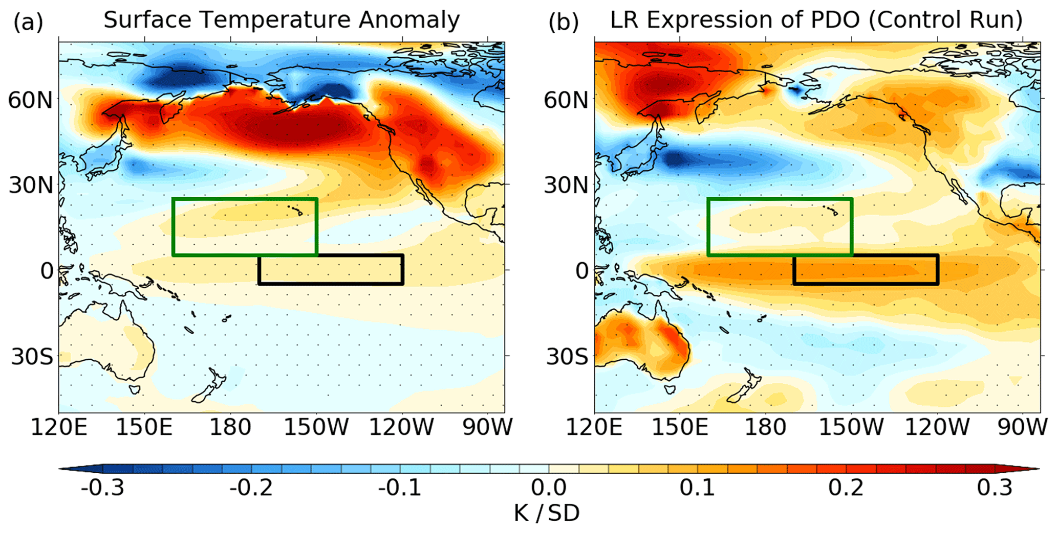
Figure 1Annual mean surface temperature anomalies for (a) ensemble mean anomaly in the nudged simulation averaged over years 1–30 and (b) linear regression (LR) onto the PDO index in the control. The anomaly between the nudged simulation and the control is projected onto the first EOF from the control run to generate a pseudo-PC. The anomaly is divided by the pseudo-PC to calculate the anomaly per standard deviation of the PDO index, expressed in a similar way to that derived from control. Units are in kelvin per standard deviation. Stippling denotes anomalies that are significant at the 95 % level. Green and black boxes show the regions for the mixed-layer heat budget analysis.
2.4 PDO index
The PDO index is calculated as the first empirical orthogonal function (EOF) of monthly SST anomalies, calculated as deviations from the climatological seasonal cycle, over the region 20–65° N, 120–260° E (Mantua et al., 1997). Before calculating the leading EOF, the temperature anomalies are weighted by the square root of the cosine of latitude to account for the decrease in area towards the pole. The monthly principal component, corresponding to the PDO index, is normalised by the standard deviation to give it unit variance. The pattern of temperature anomalies that covaries with the PDO is found by linearly regressing the time series of the monthly mean temperature anomalies onto the monthly PDO index (Fig. 1b). Here we define the PDO using the common index based on the leading EOF of North Pacific SST variability. Wills et al. (2019) showed that the tropical Pacific SST anomalies associated with this index are predominantly related to high-frequency (e.g. ENSO) SST variability, while the extratropical part is related to turbulent heat flux and wind stress anomalies associated with intrinsic Aleutian Low variability. The discrepancy between the modelled and observed SST anomalies associated with the PDO index in Fig. S1 could be due to the slightly weaker than observed ENSO amplitude in the model by around 33 % (Fig. S4) (see also Blaker et al., 2021).
3.1 Surface temperature response
Figure 1a shows annual mean surface temperature anomalies in the nudged simulation expressed as a change per standard deviation (σ) of the PDO index. Here, the anomaly between the nudged simulation and the control is projected onto the first EOF from the control run to generate a pseudo-principal component (PC). The anomaly is divided by the pseudo-PC to calculate the anomaly per standard deviation of the PDO index, expressed in a similar way to that derived from the control. A horseshoe pattern of anomalous temperature extends across the North Pacific, comprising warming in the north and eastern Pacific and along the west coast of North America and cooling in the western North Pacific–KOE region. The strongest warming (0.2–0.3 K σ−1) is seen over the North Pacific and western North America. There is weaker (0.02–0.04 K σ−1) but statistically significant warming in the equatorial Pacific. Across the Pacific Ocean, the pattern of temperature anomalies in the nudged simulation closely resembles unforced multidecadal Pacific variability in the control (Fig. 1b), with a pattern correlation coefficient of 0.53. Therefore, a sustained increase in Aleutian Low strength forces a basin-wide SST response which resembles that associated with internally generated coupled variability in the control. However, there are clear differences in the sign of the anomaly outside the North Pacific basin and nudging region, such as over north-eastern Siberia and south-central USA. Furthermore, while the extratropical SST anomalies are somewhat larger in the nudged simulation, particularly in the subpolar gyre, the tropical Pacific signal is substantially weaker by a factor of ∼ 3. This indicates that atmospheric forcing by the Aleutian Low alone is not sufficient to generate a basin-wide SST response that is consistent with the intrinsic variability of the model. Note the Aleutian Low state in xref is extreme (−3σ), meaning a more realistic amplitude for sustained Aleutian Low intensification can be expected to induce a weaker response.
The seasonality of the surface temperature anomalies in the nudged simulation is shown in Fig. 2 separated for years 1–2, years 3–4, and years 5–30. The initial response to the intensified Aleutian Low is a warming in the subpolar gyre in boreal autumn (SON). This amplifies in DJF during the peak of the nudging period, where a tongue of warming extends into the subtropical North Pacific. This pattern persists into MAM after nudging ceases but is also accompanied by warming in the eastern tropical Pacific. By JJA, the tropical and subtropical temperature changes have weakened, leaving residual warming in the subpolar gyre that persists into the following winter. The temperature anomalies over land quickly dissipate due to the low specific heat capacity. A similar seasonal evolution occurs in years 3–4, but the tropical warm anomaly emerges earlier in DJF and extends further westward at its peak in MAM. The anomalies in years 5–30 show a similar spatiotemporal pattern to the first 4 years, suggesting the mechanisms by which the anomalies manifest do not evolve strongly when the signals are maintained over multi-year timescales. Small differences between years 1–4 and 5–30 are the extent of the robust signal in the tropical Pacific; there is a small reduction in the amplitude of the tropical warming in JJA and no significant western tropical Pacific warming in MAM for years 5–30. The signal of peak tropical warming in MAM in the nudged simulation qualitatively agrees with observed low-frequency Pacific variability (Fig. S1), though we note that FORTE2.0 shows a narrower band of tropical warming compared to observations. Furthermore, the weak (up to ∼ 10× weaker) footprint of modelled PDO variability in the equatorial Pacific (Fig. S1) is consistent with a notion that Aleutian Low-driven SST variability in the extratropics has little influence on tropical variability (Wills et al., 2019; Zhao et al., 2021).
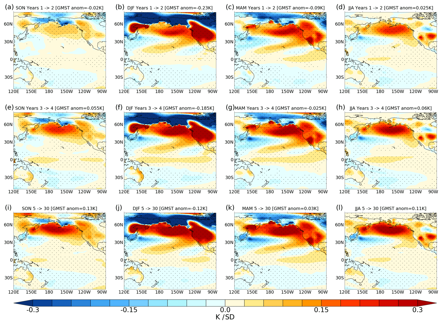
Figure 2Seasonal mean surface temperature anomalies in the nudged simulation expressed per unit PDO index [K σ−1] for SON, DJF, MAM, and JJA. Composite anomalies are shown for years 1–2 (a–d), years 3–4 (e–h), and years 5–30 (i–l). Global mean surface temperature anomalies are shown in the header. Stippling denotes anomalies that are significant at the 95 % level.
3.2 Mixed-layer heat budget
The mixed-layer heat budget in the subtropical North Pacific and Niño 3.4 regions shows different annual cycles in the anomalous temperature tendencies (Fig. 3a, b). The largest anomalous surface temperature tendency in the subtropical North Pacific occurs during the nudging period (DJF), whereas the peak warming tendency in the Niño 3.4 region occurs in February–April. In the subtropics in winter, warming from vertical diffusion is offset by meridional advection. In contrast in the Niño 3.4 region, anomalous meridional advection contributes to a warming tendency year-round, with the maximum (∼ 0.3 K month−1) in MAM. This warming is partly offset by anomalous vertical diffusion and convection. Meridional advection therefore contributes to cooling in the subtropical North Pacific but causes warming in the Niño 3.4 region.
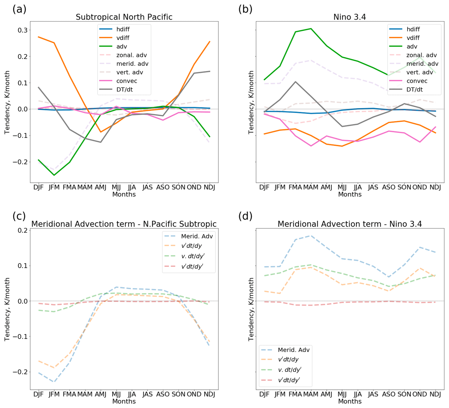
Figure 3Years 1–30, 3-month moving average of the anomalous nudged simulation minus the control mixed-layer temperature tendencies and constituent heat budget terms for the (a) subtropical North Pacific and (b) Niño 3.4 regions. Panels (c) and (d) show the meridional advection term and its linear expansion. The subtropical North Pacific and Niño 3.4 domains are indicated by the boxes in Fig. 1.
The anomalous meridional advection in the subtropical North Pacific is dominated by the change in meridional velocity, whilst in the Niño 3.4 region the change in meridional temperature gradient is the largest contributor throughout most of the year (apart from September–December) (Fig. 3c, d). The enhanced warming tendency from February–June in the Niño 3.4 region is driven by changes in meridional velocity. The difference in contributing terms implies different mechanisms governing the changing mixed-layer temperatures in the two regions.
The net surface heat flux anomalies in the nudged simulation are shown in Fig. 4a–d. There are positive (downward) net surface heat flux anomalies across the North Pacific and within a SW–NE-oriented band in the subtropical North Pacific. The largest heat flux anomalies occur during DJF, with values in excess of 4 W m−2 σ−1. The net surface heat flux anomalies in the nudged simulation are dominated by the latent heat flux (Fig. 4e–h). The pattern of surface latent heat flux anomalies in JJA in the extratropical North Pacific represents a damping of the SST anomalies; positive flux anomalies extend eastward from the KOE region, which are enveloped by negative anomalies in the northeast Pacific and subtropical North Pacific. The positive heat fluxes exhibited in the KOE region in all seasons outside of DJF are evidence that cold SST anomalies in this region reduce heat loss to the atmosphere throughout the simulations. Regions such as those in the north-eastern North Pacific appear to dampen the SST anomalies during MAM and JJA, which may indicate limited dynamic feedback to the atmosphere. However, across the central North Pacific, the persistence of surface latent flux anomalies year-round is expected given the surface temperature persistence and alludes to ocean–atmosphere feedbacks.
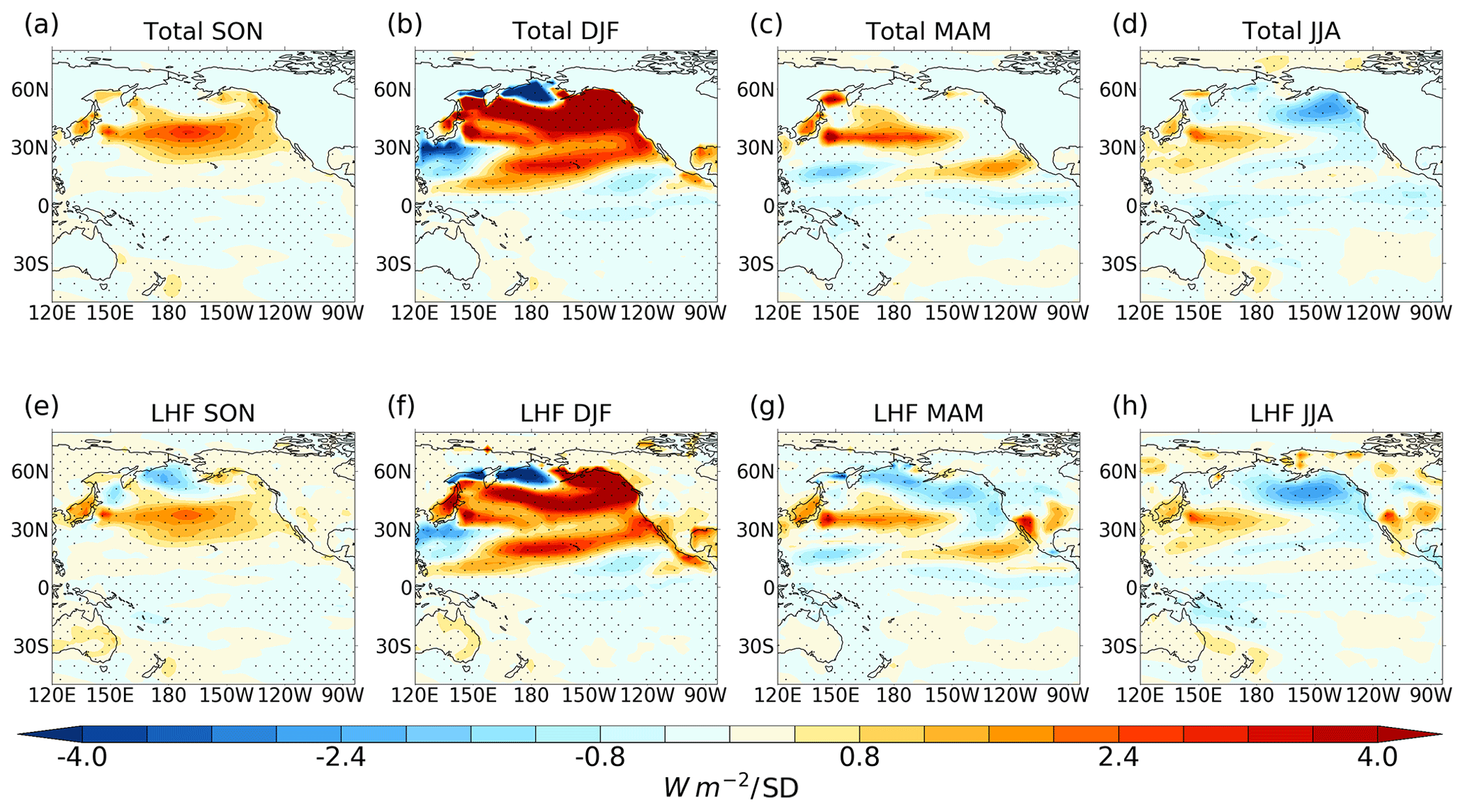
Figure 4(a–d) Years 1–30 seasonal mean net surface heat flux anomalies in the nudged simulation. (e–h) Years 1–30 seasonal mean latent heat flux anomaly in the nudged simulation. Positive denotes downward flux. Stippling denotes anomalies that are statistically significant at the 95 % level. Units: W m−2 per standard deviation.
3.3 Atmospheric circulation response
Figure 5 shows the seasonal mean zonal and meridional near-surface wind anomalies in the nudged simulation. As expected, the largest anomalies occur in the period over which nudging is applied (DJF), with a westerly zonal wind anomaly of up to ∼ 0.5 m s in the subtropics and an easterly anomaly of a similar magnitude in the subpolar extratropics. The meridional wind shows alternating southerly–northerly anomalies across the North Pacific orientated with a north-easterly tilt, suggesting that a persistently strong Aleutian Low invokes a modulation of the climatological Rossby wave train, providing a pathway for atmospheric communication between the North Pacific and eastern tropical Pacific. Evidence for the modulation of the Rossby wave train is further evident in the upper-tropospheric winds (Fig. S5). Recall that the nudging strength in the upper troposphere is several times weaker than at the surface (Fig. S2), so the upper-level circulation anomalies likely represent a response to the lower-tropospheric forcing. The subtropical zonal wind anomalies represent a southerly shift of the westerlies compared to the climatology in the control, with persistent anomalies extending into the spring after nudging ceases (April – not shown). Interestingly, there is an emergence of a westerly wind anomaly near the coast of Central America in DJF that extends southward and westward into the equatorial Pacific in MAM. Although zonal wind anomalies are evident in JJA, they are not strongly statistically significant.
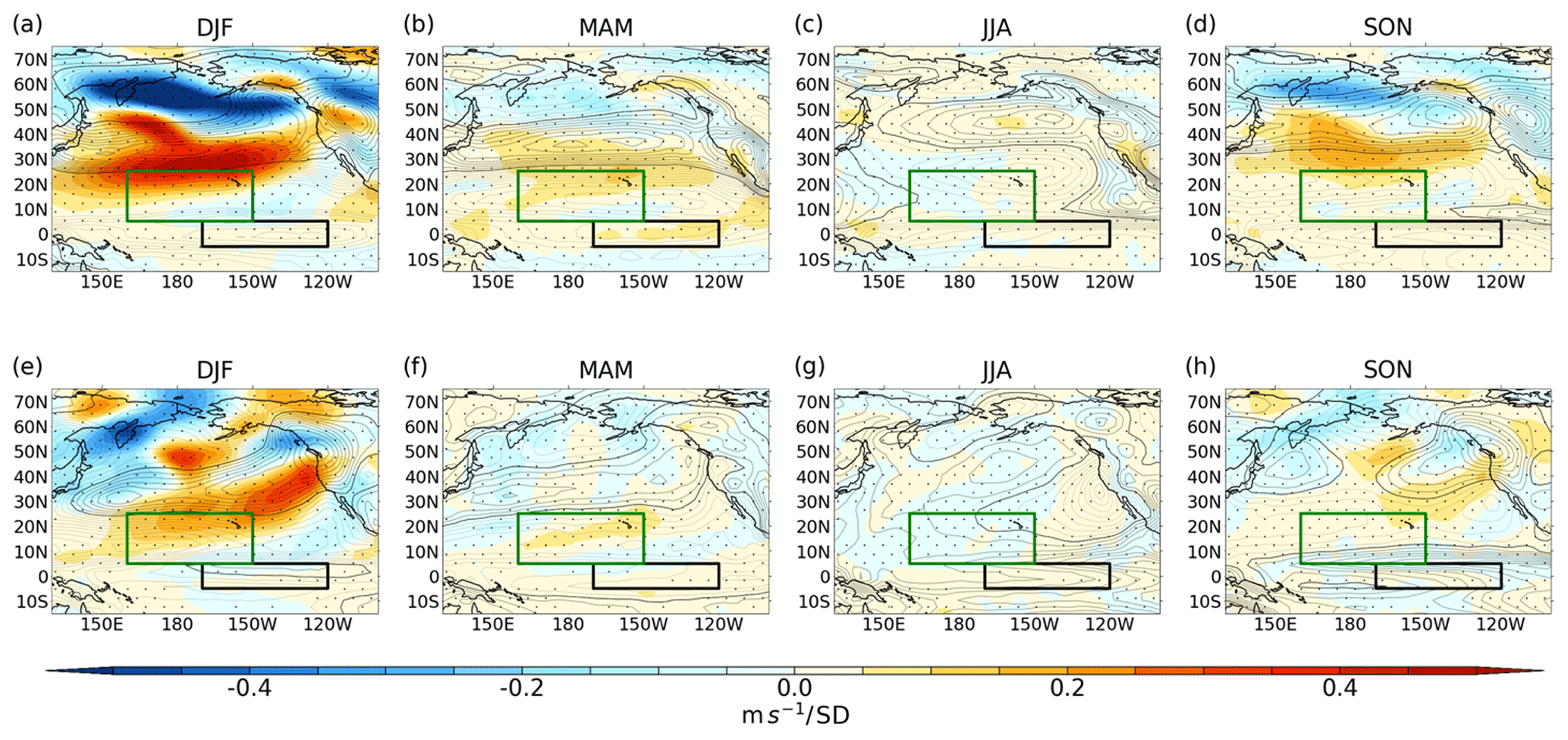
Figure 5Years 1–30 seasonal mean nudged-minus-control near-surface (lowest model level) wind anomalies for (a–d) zonal and (e–h) meridional wind. Contours show climatology of control (dashed lines are negative values, contour interval 1 m s−1). Stippling denotes anomalies that are significant at the 95 % level.
Figure 6 shows the latitude–time evolution of surface temperature, near-surface wind, and surface pressure anomalies in the nudged simulation averaged over the central and eastern tropical Pacific (which is entirely outside the nudging region). There is year-round warming in subtropical and equatorial regions, with the largest magnitude in the subtropics from November through April (∼ 0.05 K σ−1) and in the equatorial region from March through July (∼ 0.3 K σ−1). The nudging invokes concurrent warming in the subtropics, while there is a seasonal delay in the emergence of warming in the equatorial Pacific. From July to November in the subtropics (around 15° N) there is substantially less warming than during the rest of the year, with values close to zero. The westerly wind anomalies coincide with the timing of the temperature anomalies, with south-westerly anomalies of ∼ 0.05 m s in the subtropics and ∼ 0.03 m s in the equatorial region. In addition to the cross-equatorial temperature gradient generated by the subtropical anomaly, the lower surface pressure in the northern subtropics (∼ 1.5 hPa), which is largest in February and March, creates a pressure gradient across the Equator, a key component of the wind–evaporation–SST (WES) mechanism. At this time there is evidence of cooling in the southern subtropics (south of 15° S).
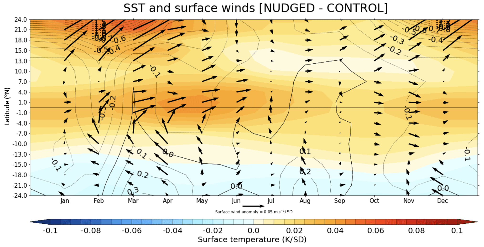
Figure 6Years 1–30 latitude–time section of nudged-minus-control SST anomaly (K σ−1: shading), surface pressure (hPa σ−1: contours), and near-surface wind anomaly (m s−1 σ−1: vectors) averaged over the central-eastern tropical Pacific (205–80° W).
The impact of an intensified Aleutian Low on the tropical Pacific in this study suggests an excitation of the seasonal footprinting mechanism (SFM) (e.g. Vimont et al., 2003; Alexander et al., 2010; Chen and Yu, 2020; Sun and Okumura, 2019). In accordance with the SFM, the SST anomalies persist into the summer season, with anomalous temperatures found in the North Pacific year-round. The signals in winter and spring show a similar spatial signature to that found by Liguori and Di Lorenzo (2019), who show an SST signature in the subtropics as a precursor to ENSO dynamics. Here we find a similar effect on multi-year timescales in response to an anomalous Aleutian Low.
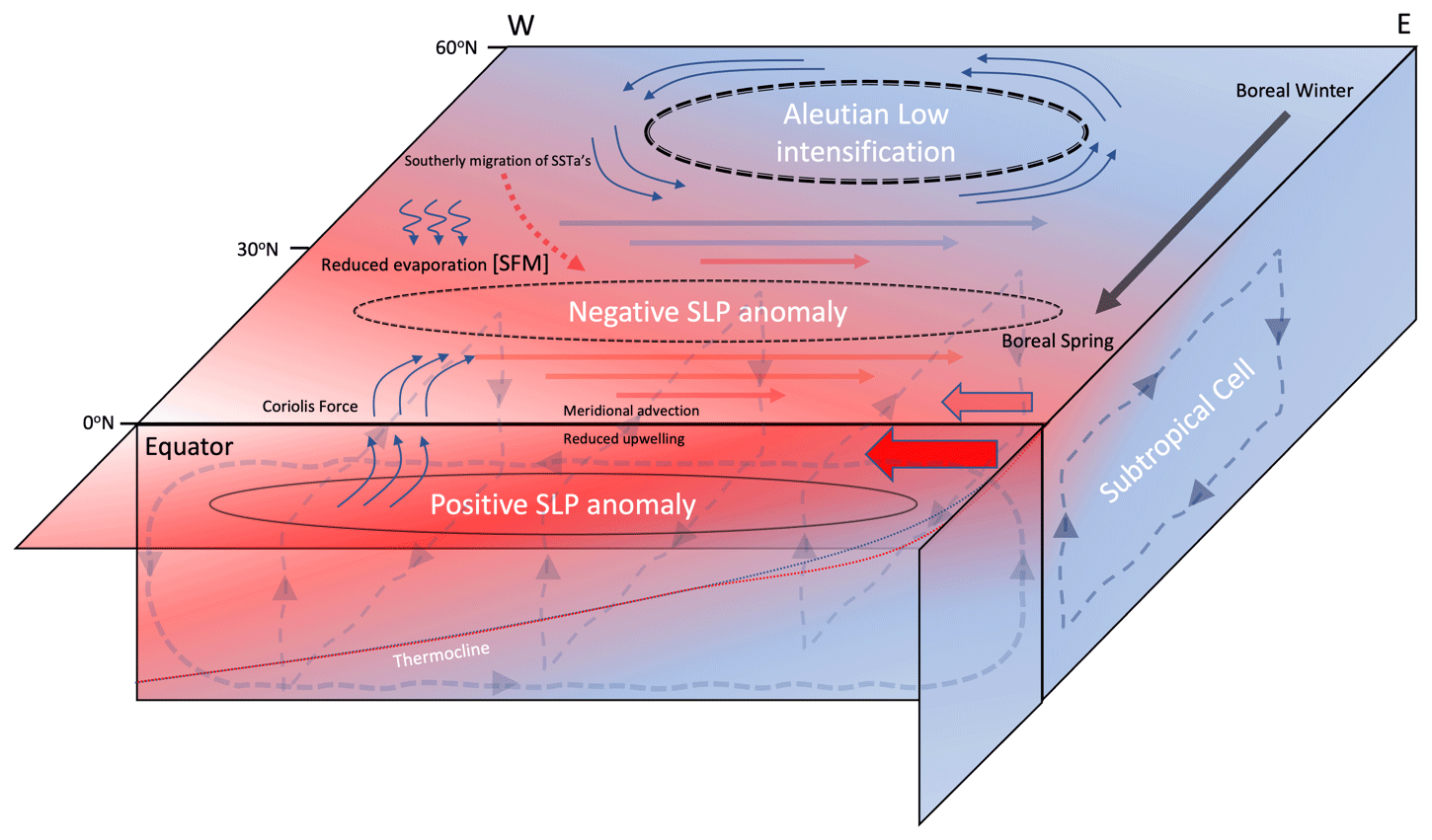
Figure 7Schematic depicting the mechanisms involved in the tropical SST anomalies manifest as a result from an intensification of the Aleutian Low. An intensified Aleutian Low (dashed black line) imposed during boreal winter is associated with intensified westerlies (reduced easterlies; solid arrows) in the subtropics and downward latent heat transfer. The migration of the SST anomalies southward during boreal winter is associated with westerly anomalies in the subtropics (reduced trades). The westerly anomalies act to weaken the background trades (filled red arrow), which reduces latent heating cooling due to decreased evaporation and hence an increase in subtropical Pacific SSTs. In the season after nudging, the temperature asymmetry about the Equator induces a sea level pressure (SLP) gradient (solid line – positive SLP; dashed line – negative SLP) that drives southerly winds across the Equator. The Coriolis force acts to turn the southerly winds in the Southern Hemisphere westward and in the Northern Hemisphere eastward. When these anomalous winds are imposed on the background easterly trade winds (filled red arrows), the southerlies south of the Equator increase the wind speed and therefore evaporative cooling, whilst north of the Equator the background trades are weakened, reducing evaporative cooling. The westerly wind anomalies along the Equator deepen the thermocline in the eastern tropical Pacific (dotted red line) and reduce upwelling/divergence of cooler waters at the Equator.
The midlatitude westerly winds show a southerly shift throughout the year which, in agreement with Liu et al. (2021), acts to prevent heat loss from the surface in the northern subtropics due to reduced evaporation. This in turn drives the SST anomaly towards the Equator. Liu et al. (2021) show the SFM as the mechanism that propagates SST anomalies southward, through a change in latent heat fluxes. However, in DJF the westerly winds imposed by the nudging cause a weakening of the subtropical trades; hence the southerly shift of westerlies starts to occur within the season of nudging. We show anomalous latent heat flux is responsible for the change in subtropical North Pacific SSTs. The limitation of the Liu et al. (2021) study is that the atmosphere was coupled to a thermodynamic slab ocean, whereas we integrate a fully coupled ocean model, allowing for a role of ocean dynamical feedbacks. Sun and Okumura (2019) conducted a related investigation by imposing heat flux anomalies associated with the North Pacific Oscillation (NPO), but they imposed a fixed year-round anomaly, whereas the Aleutian Low shows strongest variability in winter. Therefore, we only impose relaxation during boreal winter in our experimental design. The simulations presented use an anomalous Aleutian Low state taken from a single month (Fig. S3). An area for future research is to impose a suite of varying Aleutian Low states with different spatial and temporal profiles to test the sensitivity of the responses described here to details of the imposed relaxation state.
In the tropical Pacific, the dominant mechanism responsible for the increase in SSTs is meridional advection, with the change to meridional current velocity driving the accelerated warming in boreal spring. This coincides with an anomalous northward cross-equatorial SST gradient and the development of an anomalous cross-equatorial southward pressure gradient. Cross-equatorial winds are generated, which, due to Coriolis force act to weaken the trades in the northern equatorial region, decreasing the surface latent heat flux and leading to a local warming. The heat budget analysis shows that surface heat fluxes are the primary warming agent during the nudging period, whereas a change to surface advection drives the warming in the central near-equatorial Pacific. A comprehensive review of this mechanism, commonly referred to as the WES mechanism, is provided in Mahajan et al. (2009). Further, the mechanism has been posited as a pathway through which North Pacific SSTs can influence ENSO variability (Amaya et al., 2019). The equatorial thermocline depth shows a slight deepening of the thermocline in all seasons apart from SON, which is supported by changes in the vertical advection term (not shown). Figure 7 gives a pictorial representation of the combined mechanisms involved in translating the Aleutian Low anomaly into the deep tropics.
While the results make conceptual sense and are in broad agreement with studies using more comprehensive modelling tools (see earlier references), the amplitude of the response could be verified in other more detailed coupled climate models. The coarseness of the coupled model, specifically the vertical dimension of the oceanic component, is a limitation of the study. Furthermore, the model's relatively low resolution and inability to resolve mesoscale processes in the ocean and atmosphere may affect the results of the study. Future studies using observations and higher-resolution GCMs to test the results herein would be valuable. Furthermore, to ensure model stability, the anomalous nudging state was drawn from the coupled atmosphere–ocean control simulation. The Aleutian Low variability sampled from this simulation therefore includes effects from tropical variability. The month used as the reference state for the nudging coincides with an ENSO state (magnitude = 0.55) in the tropical Pacific. Further studies could investigate more idealised Aleutian Low states and their effects on extratropical–tropical communication.
Externally forced Aleutian Low trends have been implicated as a potential driver of recent variations in the Pacific Decadal Oscillation (Smith et al., 2016; Dittus et al., 2021). Here, we have investigated the potential influence of Aleutian Low trends on basin-wide low-frequency Pacific sea surface temperature variability using nudging simulations in an intermediate-complexity climate model. The target Aleutian Low state represents an extremely intense Aleutian Low state (−3σ of winter monthly variability) applied during boreal winter. The intensified Aleutian Low induces a basin-wide SST response that resembles the model's internally generated PDO with a comparable amplitude in the extratropics but a substantially weaker amplitude in the equatorial Pacific by a factor of 4 to 5. The pattern of SST variability exhibited across the basin is evident on interannual timescales as well as throughout the duration of the 30-year simulation.
The findings presented here support that the PDO can, at least in part, be driven by remotely forced changes in the North Pacific atmospheric circulation independent of the tropics. However, in our experiment the amplitude appears to be too weak to fully explain a multi-annual shift in the PDO across the tropics. This suggests that the hypothesis posed by Smith et al. (2016) that anthropogenically forced changes in the Aleutian Low drove the observed shift in the phase of the basin-wide PDO in the late 20th and early 21st centuries should be revisited.
The nudging code used in the analysis can be found here: https://doi.org/10.5281/zenodo.8142714 (Blaker et al., 2023).
Underlying model data found in this paper are available from the corresponding author upon request. HadISST data are available here: https://www.metoffice.gov.uk/hadobs/hadisst/data/download.html (Rayner et al., 2003).
The supplement related to this article is available online at: https://doi.org/10.5194/wcd-5-357-2024-supplement.
WJD and ACM designed the study. WJD developed the nudging code in FORTE2.0 with support from CMM, MMJ, and RR. ATB and RR helped with installation of FORTE2.0 at Leeds. WJD performed the analysis and produced the figures. WJD and ACM wrote the manuscript with comments from all authors. All simulations were performed on the ARC4 HPC at the University of Leeds.
The contact author has declared that none of the authors has any competing interests.
Publisher’s note: Copernicus Publications remains neutral with regard to jurisdictional claims made in the text, published maps, institutional affiliations, or any other geographical representation in this paper. While Copernicus Publications makes every effort to include appropriate place names, the final responsibility lies with the authors.
We are grateful to Paloma Trascasa-Castro for discussion of ENSO processes and to John Marsham and Laura Wilcox for feedback on an earlier version of the manuscript.
This research has been supported by the Natural Environment Research Council (grant no. NE/L002574/1) and the European Union’s Horizon 2020 Research and Innovation Programme (grant no. 820829, CONSTRAIN project). Amanda C. Maycock received funding from The Leverhulme Trust.
This paper was edited by David Battisti and reviewed by two anonymous referees.
Alexander, M. A., Vimont, D. J., Chang, P., and Scott, J. D.: The impact of extratropical atmospheric variability on ENSO: Testing the seasonal footprinting mechanism using coupled model experiments, J. Climate, 23, 2885–2901, https://doi.org/10.1175/2010JCLI3205.1, 2010.
Amaya, D. J., Kosaka, Y., Zhou, W., Zhang, Y., Xie, S. P., and Miller, A. J.: The North Pacific pacemaker effect on historical ENSO and its mechanisms, J. Climate, 32, 7643–7661, https://doi.org/10.1175/JCLI-D-19-0040.1, 2019.
Blaker, A. T., Joshi, M., Sinha, B., Stevens, D. P., Smith, R. S., and Hirschi, J. J.-M.: FORTE 2.0: a fast, parallel and flexible coupled climate model, Geosci. Model Dev., 14, 275–293, https://doi.org/10.5194/gmd-14-275-2021, 2021.
Blaker, A. T., Dow, W. J., and Joshi, M. M.: NOC-MSM/FORTE2.0: FORTE 2.0: a fast, parallel and flexible coupled climate model, Zenodo [code], https://doi.org/10.5281/zenodo.8142714, 2023.
Chen, S. and Yu, B.: The seasonal footprinting mechanism in large ensemble simulations of the second generation Canadian earth system model: uncertainty due to internal climate variability, Clim. Dynam., 55, 2523–2541, https://doi.org/10.1007/s00382-020-05396-y, 2020.
Deser, C., Sun, L., Tomas, R. A., and Screen, J.: Does ocean coupling matter for the northern extratropical response to projected Arctic sea ice loss?, Geophys. Res. Lett., 43, 2149–2157, https://doi.org/10.1002/2016GL067792, 2016.
Dittus, A. J., Hawkins, E., Robson, J. I., Smith, D. M., and Wilcox, L. J.: Drivers of Recent North Pacific Decadal Variability: The Role of Aerosol Forcing, Earth's Future, 9, 12, https://doi.org/10.1029/2021EF002249, 2021.
Dow, W. J., Maycock, A. C., Lofverstrom, M., and Smith, C. J.: The effect of anthropogenic aerosols on the aleutian low, J. Climate, 34, 1725–1741, https://doi.org/10.1175/JCLI-D-20-0423.1, 2021.
Gan, B. L., Wu, F., Jia, S., Li, W., Cai, H., Nakamura, Alexander M. A., and Miller, A. J.: On the response of the Aleutian Low to greenhouse warming, J. Climate, 30, 3907–3925, https://doi.org/10.1175/JCLI-D-15-0789.1, 2017.
Hu, D. and Guan, Z.: Decadal relationship between the stratospheric arctic vortex and pacific decadal oscillation, J. Climate, 31, 3371–3386, https://doi.org/10.1175/JCLI-D-17-0266.1, 2018.
Jin, F. F.: Low-frequency modes of tropical ocean dynamics, J. Climate, 14, 3874–3881, https://doi.org/10.1175/1520-0442(2001)014<3874:LFMOTO>2.0.CO;2, 2001.
Joshi, M., Stringer, M., van der Wiel, K., O'Callaghan, A., and Fueglistaler, S.: IGCM4: a fast, parallel and flexible intermediate climate model, Geosci. Model Dev., 8, 1157–1167, https://doi.org/10.5194/gmd-8-1157-2015, 2015.
Knight, J. R., Maidens, A., Watson, P. A. G., Andrews, M., Belcher, S., Brunet, G., Fereday, D., Folland, C. K., Scaife, A. A., and Slingo, J.: Global meteorological influences on the record UK rainfall of winter 2013–14, Environ. Res. Lett., 12, 7, https://doi.org/10.1088/1748-9326/aa693c, 2017.
Knutson, T. R. and Manabe, S.: Model assessment of decadal variability and trends in the tropical Pacific Ocean, J. Climate, 11, 2273–2296, https://doi.org/10.1175/1520-0442(1998)011<2273:MAODVA>2.0.CO;2, 1998.
Kwon, Y. O. and Deser, C.: North Pacific decadal variability in the community climate system model version 2, J. Climate, 20, 2416–2433, https://doi.org/10.1175/JCLI4103.1, 2007.
Latif, M. and Barnett, T. P.: Decadal climate variability over the North Pacific and North America: Dynamics and predictability, J. Climate, 9, 2407–2423, https://doi.org/10.1175/1520-0442(1996)009<2407:DCVOTN>2.0.CO;2, 1996.
Liguori, G. and Di Lorenzo, E.: Separating the North and South Pacific Meridional Modes Contributions to ENSO and Tropical Decadal Variability, Geophys. Res. Lett., 46, 906–915, https://doi.org/10.1029/2018GL080320, 2019.
Mantua, N. J., Hare, S. R., Zhang, Y., Wallace, J. M., and Francis, R. C.: A Pacific Interdecadal Climate Oscillation with Impacts on Salmon Production, B. Am. Meteorol. Soc., 78, 1069–1079, https://doi.org/10.1175/1520-0477(1997)078<1069:APICOW>2.0.CO;2, 1997.
Mahajan, S., Saravanan, R., and Chang, P.: The role of the wind-evaporation-sea surface temperature (WES) feedback in air-sea coupled tropical variability, Atmos. Res., 94, 19–36, https://doi.org/10.1016/j.atmosres.2008.09.017, 2009.
Martin, Z., Orbe, C., Wang, S., and Sobel, A.: The MJO–QBO relationship in a GCM with stratospheric nudging, J. Climate, 34, 4603–4624, https://doi.org/10.1175/JCLI-D-20-0636.1, 2021.
Nagano, A. and Wakita, M.: Wind-driven decadal sea surface height and main pycnocline depth changes in the western subarctic North Pacific, Progress in Earth and Planetary Science, 6, 1–26, https://doi.org/10.1186/s40645-019-0303-0, 2019.
Newman, M., Alexander, M. A., Ault, T. R., Cobb, K. M., Deser, C., Di Lorenzo, E., Mantua, N. J., Miller, A. J., Minobe, S., Nakamura, H., Schneider, N., Vimont, D. J., Phillips, A. S., Scott, J. D., and Smith, C. A.: The Pacific decadal oscillation, revisited, J. Climate, 29, 4399–4427, https://doi.org/10.1175/JCLI-D-15-0508.1, 2016.
Pickart, R. S., Moore, G. W. K., Macdonald, A. M., Renfrew, I. A., Walsh, J. E., and Kessler, W. S.: Seasonal evolution of Aleutian low pressure systems: Implications for the North Pacific subpolar circulation, J. Phys. Oceanogr., 39, 1317–1339, https://doi.org/10.1175/2008JPO3891.1, 2009.
Rayner, N. A., Parker, D. E., Horton, E. B., Folland, C. K., Alexander, L. V., Rowell, D. P., Kent, E. C., and Kaplan, A.: Global analyses of sea surface temperature, sea ice, and night marine air temperature since the late nineteenth century, J. Geophys. Res., 108, 4407, https://doi.org/10.1029/2002JD002670, 2003 (data available at: https://www.metoffice.gov.uk/hadobs/hadisst/data/download.html).
Richter, J. H., Deser, C., and Sun, L.: Effects of stratospheric variability on El Niño, Environ. Res. Lett., 10, 12, https://doi.org/10.1088/1748-9326/10/12/124021, 2015.
Schneider, N. and Cornuelle, B. D.: The forcing of the Pacific Decadal Oscillation, J. Climate, 18, 4355–4373, https://doi.org/10.1175/JCLI3527.1, 2005.
Simon, A., Gastineau, G., Frankignoul, C., Rousset, C., and Codron, F.: Transient climate response to Arctic Sea ice loss with two ice-constraining methods, J. Climate, 34, 3295–3310, https://doi.org/10.1175/JCLI-D-20-0288.1, 2021.
Smith, D. M., Booth, B. B. B., Dunstone, N. J., Eade, R., Hermanson, L., Jones, G. S., Scaife, A. A., Sheen, K. L., and Thompson, V.: Role of volcanic and anthropogenic aerosols in the recent global surface warming slowdown, Nat. Clim. Change, 6, 936–940, https://doi.org/10.1038/nclimate3058, 2016.
Sun, J. and Wang, H.: Relationship between Arctic Oscillation and Pacific Decadal Oscillation on decadal timescale, Chinese Sci. Bull., 51, 75–79, https://doi.org/10.1007/s11434-004-0221-3, 2006.
Sun, T. and Okumura, Y. M.: Role of stochastic atmospheric forcing from the south and North Pacific in tropical Pacific decadal variability, J. Climate, 32, 4013–4038, https://doi.org/10.1175/JCLI-D-18-0536.1, 2019.
Terray, L., Valcke, S., and Piacentini, A.: OASIS 2.3 Ocean Atmosphere Sea Ice Soil, User’s Guide and Reference Manual, Technical Report TR/CMGC/99-37, CERFACS, Toulouse, France, 1999.
Trenberth, K. E. and Hurrell, J. W.: Decadal atmosphere-ocean variations in the Pacific, Clim. Dynam., 9, 303–319, https://doi.org/10.1007/BF00204745, 1994.
Vimont, D. J.: The contribution of the interannual ENSO cycle to the spatial pattern of decadal ENSO-like variability, J. Climate, 18, 2080–2092, https://doi.org/10.1175/JCLI3365.1, 2005.
Vimont, D. J., Wallace, J. M., and Battisti, D. S.: The seasonal footprinting mechanism in the Pacific: Implications for ENSO, J. Climate, 16, 2668–2675, https://doi.org/10.1175/1520-0442(2003)016<2668:TSFMIT>2.0.CO;2, 2003.
Watson, P. A. G., Weisheimer, A., Knight, J. R., and Palmer, T. N.: The role of the tropical West Pacific in the extreme Northern Hemisphere winter of 2013/2014, J. Geophys. Res., 121, 1698–1714, https://doi.org/10.1002/2015JD024048, 2016.
Webb, D. J.: An ocean model code for array processor computers, Comput. Geosci., 22, 569–578, https://doi.org/10.1016/0098-3004(95)00133-6, 1996.
Wills, R. C. J., Battisti, D. S., Proistosescu, C., Thompson, L. A., Hartmann, D. L., and Armour, K. C.: Ocean Circulation Signatures of North Pacific Decadal Variability, Geophys. Res. Lett., 46, 1690–1701, https://doi.org/10.1029/2018GL080716, 2019.
Zhang, Y., Xie, S. P., Kosaka, Y., and Yang, J. C.: Pacific decadal oscillation: Tropical Pacific forcing versus internal variability, J. Climate, 31, 8265–8279, https://doi.org/10.1175/JCLI-D-18-0164.1, 2018.
Zhao, Y., Newman, M., Capotondi, A., Di Lorenzo, E., and Sun, D.: Removing the effects of tropical dynamics from north pacific climate variability, J. Climate, 34, 9249–9265, https://doi.org/10.1175/JCLI-D-21-0344.1, 2021.