Mid-Pliocene not analogous to high-CO₂ climate when considering Northern Hemisphere winter variability

In this study, we address the question of whether the mid-Pliocene climate can act as an analogue for a future warm climate with elevated CO₂ concentrations, specifically regarding Northern Hemisphere winter variability. We use a set of sensitivity simulations with the global coupled climate model CESM1.0.5 (CCSM4-Utr), which is part of the PlioMIP2 model ensemble, to separate the response to a CO₂ doubling and to mid-Pliocene boundary conditions other than CO₂. In the CO₂ doubling simulation, the Aleutian low deepens, and the Pacific–North American pattern (PNA) strengthens. In response to the mid-Pliocene boundary conditions, sea-level pressure variance decreases over the North Pacific, the PNA becomes weaker and the North Pacific Oscillation (NPO) becomes the dominant mode of variability. The mid-Pliocene simulation shows a weak North Pacific jet stream that is less variable in intensity but has a high level of variation in jet latitude, consistent with a dominant NPO and indicating that North Pacific atmospheric dynamics become more North Atlantic-like. We demonstrate that the weakening of the Aleutian low, and subsequent relative dominance of the NPO over the PNA, is related to shifts in tropical Pacific convection. Variability in the North Atlantic shows little variation between all simulations. The opposite response in North Pacific winter variability to elevated CO₂ or mid-Pliocene boundary conditions demonstrates that the mid-Pliocene climate cannot serve as a future analogue in this regard.

1 Introduction

Our present climate is warming due to humans increasing the concentration of greenhouse gases in the atmosphere, and making accurate projections of our future climate is an important necessity. Future climate is dependent on the emission pathway we choose and is determined by the response of the climate system itself, including feedbacks and natural variability, to increased CO₂. One way of investigating the response of the climate system to warm conditions is by looking at the past. We can use equilibrium climate model simulations to investigate the climate response to elevated levels of atmospheric CO₂. The geological past was in equilibrium with forcing on climatological timescales and saw multiple periods with elevated atmospheric CO₂ and temperatures of which there is a reasonable amount of geological evidence and reconstructions (see also Chen et al., 2021, FAQ1.3). The most recent period with similar CO₂ concentrations to the present day was the mid-Pliocene warm period, approximately 3 Ma (Tierney et al., 2020). It had a similar geography – compared to earlier geological warm periods – to the present day. The most notable differences include a reduction of the Greenland and West Antarctic ice sheets as well as a closure of the Bering Strait and Canadian Arctic Archipelago. It has been called the “best analogue” for near-future climate, because surface temperatures at the end of this century would be most similar to mid-Pliocene temperatures, both following the RCP4.5 and RCP8.5 scenarios, compared to other past climate periods (Burke et al., 2018).

The mid-Pliocene has been investigated using coupled climate models as part of two phases of the Pliocene Model Intercomparison Project (PlioMIP). The most recent PlioMIP2 employs a time-slice approach in order to compare model simulations and proxy reconstructions in a detailed way. Several model–data comparisons and ensemble investigations have been done in the PlioMIP2, for example, concerning general mean climate (Haywood et al., 2020), the global hydrological cycle (Han et al., 2021), Arctic warming (De Nooijer et al., 2020), the Atlantic meridional overturning circulation (AMOC,  Zhang et al., 2020; Weiffenbach et al., 2023) and the El Niño–Southern Oscillation (ENSO,  Oldeman et al., 2021; Pontes et al., 2022). Some of these studies show very different climate responses to the forcing changes in the mid-Pliocene compared to near-future projections, for example, a stronger AMOC (Weiffenbach et al., 2023) compared to a weakening of the AMOC in the projected future, as well as strongly reduced ENSO variability (Oldeman et al., 2021), which is not projected for near-future climate.

The equilibrated mid-Pliocene climate response might be more suited to compare with long-term future climate projections than near-future projections which are still in a transient state. For example, the mid-Pliocene saw atmospheric CO₂ concentration of 400 ppm, which is similar to the equilibrated levels of the SSP1-2.6 scenario in the year 2300 (Chen et al., 2021). Also, Haywood et al. (2020) find a PlioMIP2 mean surface temperature increase of 3.2 °C, which is similar to the global average warming of the RCP4.5 scenario in the year 2400 (Lyon et al., 2022). On even longer timescales, Feng et al. (2022) argue that the mid-Pliocene changes in ice sheets and vegetation are a long-term Earth system feedback to elevated atmospheric CO₂.

But some Pliocene boundary conditions will not be shared in a future climate, including the closure of the Bering Strait and the Canadian Arctic Archipelago. So, when considering the mid-Pliocene as a future analogue, we should consider the climate response or sensitivity to each boundary condition. Burton et al. (2023) use a linear fractionation method to show that CO₂ is the most important forcing for global surface temperatures and precipitation in the mid-Pliocene, employing a set of sensitivity studies of a selection of PlioMIP2 model contributions. However, especially at high latitudes surface temperatures respond more strongly to other boundary conditions than CO₂. This agrees with earlier work by Otto-Bliesner et al. (2017) as well as Chandan and Peltier (2018) that shows large sensitivity of the northern-high-latitude mid-Pliocene climate to closed Arctic gateways, which induce a larger surface temperature and sea-ice response than the reduced Greenland Ice Sheet or elevated atmospheric CO₂.

Apart from studying mean climate response in a warm past climate, it is useful to study the response of climate variability. Since contemporary climate change is transient, it is hard to assess changes to modes of variability that operate on interannual and decadal timescales. Investigating climate variability in equilibrated simulations can help to separate internal variability changes to the forced response from transient trends. Within the PlioMIP2, most of the attention to climate variability has focused on ENSO (Oldeman et al., 2021; Pontes et al., 2022), which was found to be reduced in amplitude in a large majority of the models, consistent with findings from the earlier PlioMIP1 ensemble (Brierley, 2015). Earlier work by Hill et al. (2011) shows reduced Northern Annular Mode (NAM) variability in the Pliocene, which was primarily attributed to the reduced height of the Rocky Mountains in the model simulations. Both PlioMIP1 and PlioMIP2 employed a time slice where the Rocky Mountain uplift had already occurred.

A feature where future climate projections fail to give a consistent response to increasing CO₂ levels is atmospheric variability in the Northern Hemisphere winter, specifically the Arctic Oscillation (AO; also referred to as the NAM) and its regional expression, the North Atlantic Oscillation (NAO) (Eyring et al., 2021). These modes represent an oscillation of mass between the subpolar latitudes and subtropics in the Northern Hemisphere and are the leading modes of sea-level pressure (SLP) variability in the northern extratropics (Ambaum et al., 2001; Hurrell and Deser, 2010). Apart from the NAO, a less pronounced mode of SLP variability operates in the North Atlantic, namely the East Atlantic (EA) pattern, which usually has its center of action over the British isles (Barnston and Livezey, 1987). The NAO plays a significant role in North Atlantic and European climate, for example, in extratropical storm tracks, and affects projections of temperature and precipitation on an interannual to decadal timescale (Deser et al., 2017; Iles and Hegerl, 2017). Uncertainties in climate projections over the Euro-Atlantic sector are largely related to atmospheric circulation variability (Woollings, 2010; Shepherd, 2014; Fereday et al., 2018), in particular because there is no consensus on how the AO and NAO respond to increasing CO₂ concentrations (Eyring et al., 2021). This is in part due to the large amplitude of internal variability related to the NAO compared to the amplitude of global warming (Osborn, 2004), as well as a considerable model spread in climate change simulations (Eyring et al., 2021). Though climate models are considered skillful in simulating the spatial features and variance of the present-day and historical NAO (Eyring et al., 2021), CMIP5 and CMIP6 models underestimate NAO variability and North Atlantic jet stream variations on a multidecadal to centennial timescale (Blackport and Fyfe, 2022).

The two leading modes of atmospheric winter variability over the North Pacific are the Pacific North American (PNA) pattern and the North Pacific Oscillation (NPO) or west Pacific teleconnection (Barnston and Livezey, 1987; Linkin and Nigam, 2008). The PNA essentially captures most of the variability of the Aleutian low-pressure system and has a large influence on present-day North Pacific and North American winter climate. The NPO is strongly linked to latitudinal displacement of the Asian–Pacific jet and Pacific storm track variability, as well as the position and strength of the Aleutian low. Linkin and Nigam (2008) state that the NPO shows a strong connection to Arctic sea-ice variability, as well as variations of the North Pacific jet stream latitude. North Pacific atmospheric variability is strongly related to atmospheric Rossby wave activity (Mo and Livezey, 1986), which can be excited through tropical convection associated with ENSO variability (Hoskins and Karoly, 1981). Chen et al. (2018) investigate a large ensemble of CMIP5 simulations and find a stronger PNA under high-CO₂ forcing but no consensus on the NPO. They find that CMIP5 models reasonably simulate spatial patterns and interannual variations of the present-day and historical PNA and NPO but lack the capability to reproduce variations on a decadal timescale.

This brings us to the research question addressed in this study. Can the mid-Pliocene climate be used to determine the response of Northern Hemisphere (NH) winter atmospheric variability, such as the NAO, NAM and PNA, to increased CO₂? To answer this question, we will aim to answer two subquestions. (1) Is there a difference in the pre-industrial climate response to elevated CO₂ and to mid-Pliocene boundary conditions other than CO₂, including closed Arctic gateways and reduced ice sheets? (2) How do changes in mean winter climate relate to changes in atmospheric variability in the NH?

We will investigate NH winter variability in pre-industrial and mid-Pliocene simulations within one global climate model, the Community Earth System Model (CESM) version 1.0.5, that is a part of the PlioMIP2 ensemble. Since the equilibrated mid-Pliocene climate saw increased CO₂ levels as well as different boundary conditions such as topography, land–ice coverage and vegetation, we will use sensitivity simulations to identify the response to both boundary conditions. Starting from a pre-industrial reference simulation with present-day geography and 280 ppm atmospheric CO₂, we will assess the response to a CO₂ doubling (560 ppm) with present-day boundary conditions, as well as the response to mid-Pliocene boundary conditions at pre-industrial CO₂ levels (280 ppm). Both simulations represent approximately 3 °C warmer worlds but due to different forcings (Baatsen et al., 2022).

Based on earlier research, we can hypothesize what we expect the answers to our research question will be. Menemenlis et al. (2021) investigate extratropical hydroclimate changes in the mid-Pliocene using a version of CCSM4 and find large precipitation changes linked to dynamical shifts in atmospheric rivers. A wintertime stationary wave train in the pre-industrial period largely disappears in the mid-Pliocene, resulting in fewer atmospheric rivers over the eastern North Pacific region. They use sensitivity studies to show that this mean winter climate response is mainly caused by the changes in ice sheets and closed gateways and not by an increased level of atmospheric CO₂. However, they do not study variability. Oldeman et al. (2021) show that ENSO variability in the PlioMIP2 ensemble is reduced, with the largest reduction in the model we employ. This is found to be related to a shift in the mean Pacific Intertropical Convergence Zone (ITCZ) position (Pontes et al., 2022). Since ENSO variability influences the NH atmospheric circulation, including atmospheric modes of variability such as the PNA and the NAO and oceanic modes such as the Pacific Decadal Oscillation (PDO; see, e.g.,  Mo and Livezey, 1986; Yeh et al., 2018; Domeisen et al., 2019), we can expect changes to NH atmospheric variability when we know that ENSO variability is reduced.

In the following section, we explain the model and simulations used, outline our analysis methods and compare our pre-industrial simulations to reanalysis data. In Sect. 3, we present results of mean winter climate as well as SLP winter variability for all sensitivity simulations. We also investigate jet stream variations related to SLP variability in response to the mid-Pliocene boundary conditions and demonstrate how the tropical Pacific mean state is linked to changes in winter variability. Section 4 presents a physical interpretation and discussion of the results, as well as our answer to the question of the mid-Pliocene as a future analogue. A summary and outlook concludes the paper.

2 Methods and data

2.1 Model and simulations

2.1.1 Model design and configuration

The model used in this study is 1 out of 17 models in model ensemble PlioMIP2. The PlioMIP2 methodology for participating modeling groups is outlined in Haywood et al. (2016). In comparison to PlioMIP1, an enhanced set of boundary conditions is supplied (the PRISM4 reconstruction; see Dowsett et al., 2016). The experimental setup is such that it represents a specific time slice in the mid-Pliocene, the KM5c interglacial (3.205 Ma), where the orbital configuration was similar to the present day. The provided mid-Pliocene boundary conditions include mid-Pliocene topography and bathymetry, coastlines, land surface properties (i.e., vegetation, soil type and ice sheet coverage), and atmospheric composition. Some important aspects of the mid-Pliocene model geography compared to pre-industrial reference are the closure of the Bering Strait and the Canadian Arctic Archipelago (or Northwest Passage). This isolates the Arctic Ocean from the North Pacific ocean, as well as from the Labrador Sea. The Greenland Ice Sheet (GIS) is substantially reduced in spatial coverage, covering only part of southeastern Greenland and being reduced in height, affecting topography as well.

CESM is a fully coupled ocean–atmosphere–land–ice general circulation model. For specific use in paleoclimate modeling, version 1.0.5 is a suitable trade-off between model complexity and computational cost. The model version used here employs the ocean module POP2 and the atmosphere module CAM4, which is part of the Community Climate System Model version 4 (CCSM4) and can be considered a CMIP5 generation model. Within the PlioMIP2 ensemble our model is referred to as CCSM4-Utr. The atmospheric grid has a horizontal resolution of ∼ 2° (2.5° × 1.9° or 144 × 96 grid cells) and 26 vertical levels, while the ocean grid has a nominal 1° (1.25° × 0.9°) horizontal resolution. Details on the model version, simulations, spin-up and general climate features can be found in Baatsen et al. (2022).

The PlioMIP2 model contributions vary in model complexity, resolution, implementation of the provided boundary conditions and in the set of simulations performed. Each model has performed two core experiments, namely a pre-industrial reference simulation at 280 ppm CO₂ and a mid-Pliocene simulation at 400 ppm CO₂. Following the PlioMIP2 naming convention, these simulations are referred to as E²⁸⁰ and Eoi⁴⁰⁰, respectively (with the “o” and “i” referring to the implementation of Pliocene orography and ice sheets and the number referring to the atmospheric CO₂ concentration). The CCSM4-Utr has performed an additional set of sensitivity simulations, employing present-day and mid-Pliocene geography, vegetation, and ice sheets at different levels of atmospheric CO₂.

2.1.2 Performance within PlioMIP2 ensemble

Within the PlioMIP2, results of the pre-industrial E²⁸⁰ and mid-Pliocene Eoi⁴⁰⁰ simulations have been compared, both to proxy reconstructions and to other ensemble members. Haywood et al. (2020) show that CCSM4-Utr is one of the best-performing models in the PlioMIP2 regarding data–model comparison for each site. De Nooijer et al. (2020) study Arctic warming in the PlioMIP2 ensemble and find that CCSM4-Utr is one of the best-performing models considering the data–model comparison of Arctic temperature anomalies. CCSM4-Utr winter sea-ice extent also matches well with reconstructions, although seasonal sea-ice extent reconstructions are very limited. Tindall et al. (2022) show that a significant model–data bias arises in winter months, due to a potential warm bias in the data and a potential cold bias in the models, but this holds for all PlioMIP2 models.

The CCSM4-Utr mid-Pliocene Eoi⁴⁰⁰ simulations have been included in several PlioMIP2 ensemble studies. Oldeman et al. (2021) show that the amplitude of mid-Pliocene ENSO variability was reduced compared to the pre-industrial and that CCSM4-Utr has the most reduced ENSO variability of the ensemble (67 % reduction compared to 24 % in the ensemble mean). Pontes et al. (2022) also study PlioMIP2 ENSO and find a relation between the reduced ENSO and a northward shift in Pacific ITCZ. They show that CCSM4-Utr exhibits the largest northward shift of the ITCZ from October to February. Zhang et al. (2020) and Weiffenbach et al. (2023) show an increased AMOC strength in the PlioMIP2 ensemble. Weiffenbach et al. (2023) furthermore explain that models with a closed Bering Strait and Canadian Arctic Archipelago (including CCSM4-Utr) show reduced freshwater transport from the Arctic Ocean into the North Atlantic, causing an increase in subpolar North Atlantic salinity, which drives the stronger AMOC. In this case, CCSM4-Utr simulates a stronger AMOC in the mid-Pliocene with values close to the ensemble mean (22 Sv over 19 Sv in the pre-industrial reference simulation).

2.1.3 Simulation specifics

The PlioMIP2 naming convention is used for our set of sensitivity simulations. The reference simulation is the pre-industrial E²⁸⁰ with present-day boundary conditions (BCs; orography, ice sheets and vegetation) and 280 ppm atmospheric CO₂. We perform a CO₂ doubling simulation at present-day geography (E⁵⁶⁰) to investigate the effect of radiative forcing alone. We also perform a mid-Pliocene BCs simulation at pre-industrial carbon levels (Eoi²⁸⁰) to investigate the response to the mid-Pliocene orography, ice sheets and vegetation but not to CO₂. Additionally, we perform a mid-Pliocene BCs simulation at 560 ppm CO₂ (Eoi⁵⁶⁰) in order to investigate nonlinearity in the responses to the forcings. All simulations have spin-up times of around 3000 model years, and an analysis of the results of the Eoi⁴⁰⁰ simulation is found in Baatsen et al. (2022).

For the sake of consistency, we use pre-industrial and CO₂ doubling simulations that employ a paleoclimate vertical ocean diffusivity, which we also use in the mid-Pliocene simulations. The difference between this adapted E²⁸⁰ and the E²⁸⁰ that is used in most PlioMIP2 studies, as well as the motivation for using a different parametrization, is discussed in Baatsen et al. (2022). The effect of this parametrization difference was found to be very minimal on ocean surface temperatures and negligible for atmospheric variables. The CO₂ doubling simulation was also rerun with this paleo-mixing parametrization. The E²⁸⁰ and E⁵⁶⁰ simulations are spun up from equilibrated simulations and have spin-up times of 4000 and 2500 model years, respectively (details on the spin-up can be found in Fig. S1 in the Supplement).

2.2 Data analysis and methodology

In order to investigate NH winter climate and variability, we study 200 years per simulation, and we use monthly mean Januaries only. Results for December–January–February (DJF) or climatological winter were found to give very similar results for the sake of this study. The vertical levels of the model are on a hybrid sigma scheme, so results in the vertical have been interpolated onto pressure levels.

We investigate the mean state, i.e., the mean of all 200 Januaries, as well as variability on top of this mean state. We consider SLP, near-surface air temperature (SAT) and precipitation, as well as zonal winds and potential vorticity (PV) in the higher troposphere. To identify the subtropical jet stream we investigate zonal wind at 200 hPa (U₂₀₀). We also compute the location of the dynamical tropopause, here defined as the isoline of 2 PVU (potential vorticity units) at 200 hPa. We also compute the dynamical tropopause defined as the largest zonal isobaric PV gradient per longitude, but it gave very similar results to using the 2 PVU isoline. The dynamical tropopause at 200 hPa generally follows the subtropical jet stream core (Kunz et al., 2011).

To study winter climate variability we focus on the temporal behavior of SLP. Before analysis, a locally weighted scatter plot smoothing (LOWESS) using a 50-year moving window is removed from anomalies at each spatial grid point (alpha of 0.25). A window size of 50 years was chosen since we are mainly interested in interannual and decadal winter variability. Furthermore, CMIP5 models are known to underestimate variations of multidecadal periods of the winter NAO and jet stream (Blackport and Fyfe, 2022). We use empirical orthogonal function (EOF) analysis to separate the SLP variance in orthogonal modes of spatial and temporal variability. Spatial EOF patterns and their corresponding principal component (PC) time series are obtained from the LOWESS-filtered SLP anomalies and using a spatial weighting that corresponds to the cosine of the latitude. The EOF patterns are normalized using their spatial standard deviation.

We perform EOF analysis over the NH, as well as over the North Atlantic (NA, 90° W–30° E) and North Pacific (NP, 120° E–120° W) basins. The regions were chosen such that they include the centers of action of known present-day modes of climate variability, such as the AO, NAO and PNA, but also to be equal in longitudinal width. All EOF regions, including the NH, are bound in latitude between 20 and 85° N. In the NH, we only consider the first EOF, which we call the AO (we prefer AO over NAM since the AO is often defined as SLP EOF, whereas the NAM is often defined as the index of SLP anomalies). In the NA and NP regions, we consider the first and second EOF. Based on whether the spatial pattern represents a dipole or a monopole, we categorize the EOFs according their known nomenclature in the present day: the NAO (NA dipole) and EA (NA monopole) and the NPO (NP dipole) and PNA (NP monopole). The dipole/monopole characterization is done by considering the shape and amplitudes of the peaks of the zonally averaged EOF patterns. While these modes may have a different pattern or prominence in a past climate with different boundary conditions, compared to the present day, we decided to use known nomenclature, both to avoid confusion and to follow past studies of paleoclimate variability (e.g., the NAO in the last glacial maximum;  Rivière et al., 2010). The EOFs and PCs of the AO, NAO and NPO modes are defined such that the mean EOF amplitude in the region north of 75° N is positive, while the EA and PNA modes are defined such that the mean EOF amplitude in the region 50–60° N is negative. We also consider the percentage of variance explained by each EOF. We perform a variance bootstrapping method to quantify whether the variance explained per mode between two simulations has a statistically significant difference, which is defined as no overlap between the top 95 % and bottom 5 % (or vice versa) variance explained percentages obtained through the bootstrapping method.

We investigate in what way the different modes of winter variability in the whole NH and over the NP and NA basins are connected. We quantify the level of correlation by means of the Pearson correlation coefficient between the PCs of the corresponding modes. The correlation coefficient between the first and second mode in either the NP or NA will always be zero, since these EOFs are orthogonal by definition. We consider the correlation to be statistically significant when p<0.05.

We also perform an analysis of jet variations in the NP. For variations in the central NP jet stream, we limit ourselves to the 200 hPa level and the zonal mean between 160 and 220° E (or 140° W). We define jet intensity as the maximum of the zonal wind velocity in this sector and jet latitude as the latitude corresponding to this maximum. Furthermore, we investigate the jet stream in the phases of the NPO mode, where we define the NPO+ phase as the average of the highest 5 % (or 10 Januaries) of NPO PC values and the NPO− phase as the average of the lowest 5 % of NPO PC values.

Lastly, we investigate the relationship between ENSO variability, tropical convection, and the variability of SLP and the jet stream in the NP. We define ENSO variability through the Nino3.4 index, which is a measure of sea-surface temperature (SST) anomalies in the Nino3.4 region in the equatorial Pacific (5° S–5° N, 170–120° W). We characterize tropical convection using area-mean precipitation in the west-equatorial Pacific (WEP; defined as 6° S–6° N, 120–180° E). We investigate the links between variables using correlation coefficients and regression (linear slope) between variables in time. Additionally, we performed a calculation of the Rossby wave source, which is included in the Supplement.

2.3 Validation of E²⁸⁰ with reanalysis data

We compare the pre-industrial E²⁸⁰ simulation to 19th and 20th century reanalysis data. It is not a one-on-one comparison, since our pre-industrial simulation is an equilibrium scenario, while any kind of global reanalysis dataset will be influenced by human-induced climate change trends and will thus be transient. We use monthly mean sea-level pressure data from the NOAA/CIRES/DOE 20th Century Reanalysis version 3 (from here on abbreviated as CR20). The reanalysis covers the period from 1836 to 2015 and assimilates surface pressure observations in combination with a forecasting model to estimate a set of atmospheric variables. An evaluation of the performance of the CR20v3 can be found in Slivinski et al. (2021). The length of the CR20 dataset and the fact that it covers a period closer to what can be considered pre-industrial motivated us to use this reanalysis data over more recent reanalyses such as ERA5. The CR20 data are presented on a 1.0° latitude × 1.0° longitude grid, and we interpolate the data onto the model grid when computing differences between the E²⁸⁰ and CR20. The same LOWESS filtering (as with the simulation data) is applied to remove any trend due to anthropogenic climate change.

A comparison of mean SLP and the related patterns of variability between our pre-industrial simulation and reanalysis is shown in Fig. 1. Mean SLP (MSLP) is shown in Fig. 1a. The root mean squared error (RMSE) of MSLP is 5.3 hPa. Differences with the CR20 include an overestimation of the subtropical high-pressure regions, specifically over the North Atlantic and North African regions, over Central Asia, and to a smaller extent over North America (up to +12.8 hPa). A lower MSLP is simulated in the subpolar low-pressure region in the North Atlantic (up to −12.4 hPa), and the pattern extends more eastward. The North Pacific subpolar low-pressure area, the Aleutian low, is well captured in spatial extent and amplitude. Figure 1b shows SLP standard deviation (SD). SLP SD is generally overestimated in the E²⁸⁰ (mean SLP SD difference is +1.6 hPa, with an RMSE of 2.3 hPa), especially over the North Pacific and Siberian Arctic (up to +5.5 hPa). SLP SD in the North Atlantic storm track region as well as to the east of the tip of Greenland is slightly underestimated. A higher (lower) modeled SLP variance in the North Pacific (North Atlantic) in comparison to observations is a known bias for most CMIP5 and CMIP6 models (Eyring et al., 2021).

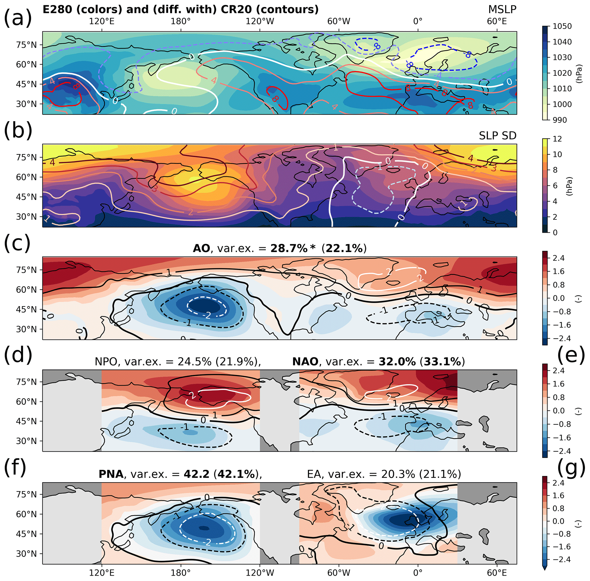
Figure 1 (a) January mean SLP and (b) SLP standard deviation (SD) for the pre-industrial reference simulation (E²⁸⁰; colors) and difference with CR20 reanalysis (E²⁸⁰ – CR20; contours). (c–g) January SLP EOFs; (c) Arctic Oscillation (AO), (d) North Pacific Oscillation (NPO), (e) North Atlantic Oscillation (NAO), (f) Pacific–North American (PNA) and (g) East Atlantic (EA) patterns, with E²⁸⁰ in colors and CR20 in contours. Percentage variance explained by each E²⁸⁰ EOF indicated (CR20 in brackets); the asterisk (^*) indicates a statistically significant difference between these. The (variance of the) leading mode in North Pacific and Atlantic regions is in bold.

Figure 1c–g show the spatial EOF patterns of SLP in the NH, NA and NP, including the percentage of variance explained for each mode. The NH mode, the AO, in Fig. 1c explains more variance in the E²⁸⁰ than in the reanalysis (28.7 % over 22.2 %), which is a statistically significant difference. The amplitudes of the North Atlantic centers of action are underestimated in the E²⁸⁰, which can be expected since the E²⁸⁰ simulated less SLP variance in that region.

The leading mode in the NP is the PNA (Fig. 1f), explaining around 42 % of SLP variance in both E²⁸⁰ and CR20. The second leading mode in the NP is the NPO (Fig. 1d), explaining 25 % (22 %) of SLP variance in the E²⁸⁰ (CR20). The E²⁸⁰ simulates both modes well in terms of spatial pattern, although the amplitude of the centers of action are a bit less pronounced and the variance more spread out over the region. The percentages of variance explained are not statistically different.

The leading mode in the NA is the NAO (Fig. 1e), explaining 32 % (33 %) of SLP variance in the E²⁸⁰ (CR20). The amplitude of the southern node is slightly underestimated, while the northern center of action is shifted towards the east. Again, this can be expected from the differences in total SLP variance as shown in Fig. 1b. The second leading mode in the NA is the EA (Fig. 1g), explaining 20 % (21 %) of SLP variance in E²⁸⁰ (CR20). The center of gravity of the strong negative node shifts eastward in the E²⁸⁰, with regards to the CR20, likely because the variance shifts more eastward in E²⁸⁰. Furthermore, where the CR20 shows that the sign of variability over Greenland is the same sign as in the center of the monopole, the E²⁸⁰ shows a clear opposite sign over Greenland. Again, also for this mode the total SLP variance in this region is underestimated. The percentages of variance explained are not statistically different.

In summary, we can say that the E²⁸⁰ pre-industrial simulation reproduces the January mean SLP as well as SLP variability from the CR20 reanalysis quite well. The modes in the North Pacific are captured well in spatial extent, amplitude and percentage of variance explained. The modes in the North Atlantic are well reproduced, albeit less accurate, especially regarding amplitudes. However, this is a likely cause of the fact that total SLP variance in the North Atlantic is reduced, which is a known bias in both CMIP5 and CMIP6 models (Eyring et al., 2021).

3 Results

3.1 Mean winter climate

3.1.1 Mean sea-level pressure and the subtropical jet stream

Figure 2 shows the January MSLP (colors) as well as mean zonal wind at 200 hPa (U₂₀₀, contours). Figure 2a shows the E²⁸⁰ MSLP results (similar to Fig. 1a but extended southward to 20° S). The January MSLP difference with E⁵⁶⁰ and Eoi²⁸⁰ is shown in Fig. 2b and c, respectively. While the MSLP response to CO₂ doubling is overall relatively small, the response to mid-Pliocene BCs is substantially larger, especially over the North Pacific. The large increase in MSLP over the NP (+16 hPa) results in a reduced MSLP difference between the NP subtropical high-pressure and subpolar low-pressure areas, as well as a slight poleward shift of the latitude with the largest MSLP gradient. MSLP, furthermore, decreases over the Arctic in the Eoi²⁸⁰ (up to −7 hPa). When comparing with the mid-Pliocene reference simulation Eoi⁴⁰⁰ (annual mean in Baatsen et al., 2022; January mean in Fig. S2), we see that the MSLP response is largely caused by the mid-Pliocene boundary conditions and not by the CO₂ increase. Only the MSLP decrease around Greenland and especially over the Baffin Bay and the Labrador Sea is a clear combination of the response to mid-Pliocene BCs and to elevated CO₂, as it can be observed both in the E⁵⁶⁰ and Eoi²⁸⁰ results.

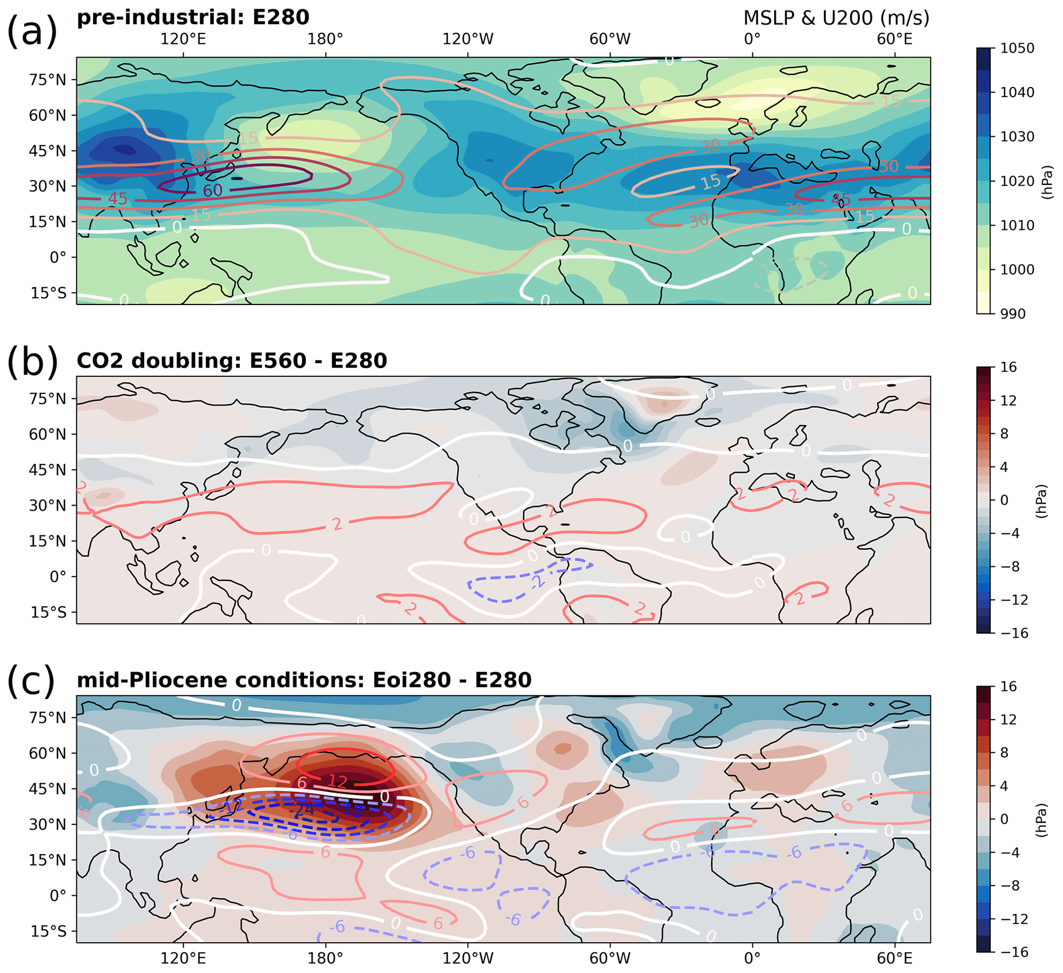
Figure 2 January mean sea-level pressure (MSLP, colors) and mean zonal wind at 200 hPa (U₂₀₀, contours) for the (a) pre-industrial reference simulation E²⁸⁰, (b) difference with CO₂ doubling E⁵⁶⁰ − E²⁸⁰ and (c) difference with mid-Pliocene boundary conditions Eoi²⁸⁰ − E²⁸⁰. Note that the increments of the color bar as well as the labels on the contour lines are slightly different between panel (b) and (c).

Figure 2a also shows E²⁸⁰ zonal wind on the 200 hPa isobar. The subtropical jet stream can clearly be identified as a streak of high zonal wind roughly between 25 and 45° N. The jet is strong and concentrated over East Asia and the North Pacific Ocean. Over the North Atlantic Ocean, two separated jet streams can be seen, roughly between 20–25 and 45–50° N. The migration of the subtropical jet towards higher latitudes over the NA, compared to the NP, corresponds to the subtropical high pressure and subpolar low pressure being more extended northwards. The E⁵⁶⁰ response in zonal wind is very minimal and limits itself to a few meters per second at most (Fig. 2b). Over the NP, a slight increase in wind speeds is found along the center of the jet. Over the Euro-Atlantic sector, the response is relatively weak. The largest increase in zonal wind in the Pacific is 4.4 m s⁻¹, which is less than the mean time variation of the E²⁸⁰ zonal wind (defined as the SD in time, 5.9 m s⁻¹). Generally, the jet stream response to the mid-Pliocene boundary conditions (Fig. 2c) is more substantial compared to the response to CO₂ doubling, with the largest response over the NP. The subtropical jet stream weakens substantially over the exit of the East Asian jet and continues to weaken over the whole of the NP, with reductions of up to 25 m s⁻¹ along the jet core, corresponding to 50 % over the central NP. Apart from the reduction in jet strength along 30° N, we also see an increase in zonal wind over the northern NP, which indicates that apart from weakening, the subtropical jet shifts or expands polewards. The weakening and widening of the North Pacific subtropical jet is consistent with the slight reduction in SLP difference between the subtropical high and subpolar low. Our findings agree with other PlioMIP2 studies; a strong increase in NP MSLP and simultaneous weakening of the NP jet stream in winter is shown in the mid-Pliocene Eoi⁴⁰⁰ simulations with CCSM4-UoT (Menemenlis et al., 2021), and a weaker NP jet stream in the annual mean is reported in Eoi⁴⁰⁰ simulations with HadCM3 and CESM2 (Hunter et al., 2019; Feng et al., 2022).

3.1.2 Surface temperatures and precipitation

Figure 3 shows the January mean surface air temperature (SAT, colors) as well as precipitation (contours). Figure 3a presents January SAT for the pre-industrial reference simulation E²⁸⁰. Arctic cold spreads far south over the continental regions, specifically Siberia and northern Canada. SAT distributions over land and the ocean are largely as expected from present-day and historical observations. The SAT difference (E⁵⁶⁰ − E²⁸⁰, Fig. 3b) shows that most continental areas warm slightly more compared to oceans at similar latitudes. Furthermore, a clear Arctic amplification signal can be observed. This response is expected with increasing atmospheric CO₂ levels (Serreze and Barry, 2011). Temperatures increase more than 15 °C over the Iceland, the Norwegian Sea and the Barents Sea. Extensive warming is furthermore found in the Labrador Sea, Bering Strait and Sea of Okhotsk. The SAT response for the Eoi²⁸⁰ is in many ways similar to the SAT response for the CO₂ doubling (Fig. 3c). An Arctic amplification response is present even without any increase in CO₂ levels. Again, we see a large warming over the Greenland Sea and Sea of Okhotsk, as well as over the Baffin Bay and Labrador Sea. In the Eoi²⁸⁰ results, we see a warmer region over the western and central North Pacific and a large area of cooling over western North America and the land bridge that is now the Bering Strait. This SAT dipole is consistent with the MSLP increase over the North Pacific and decrease over western North America as seen in Fig. 2c.

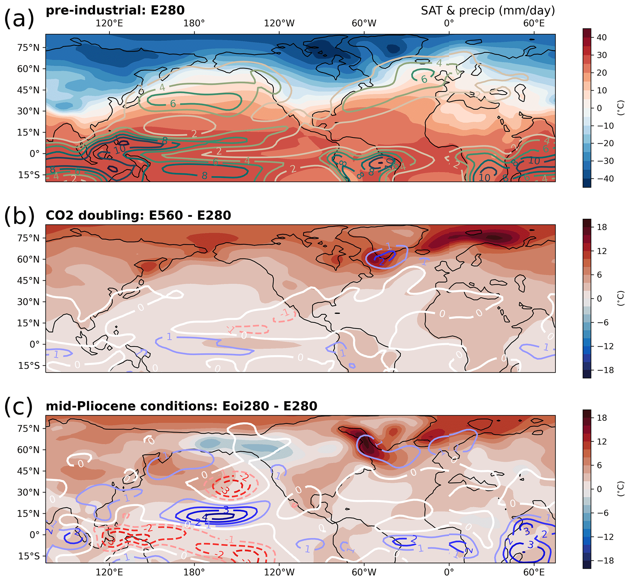
Figure 3 January mean surface air temperature (SAT, colors) and mean precipitation (precip, contours), for the (a) pre-industrial reference simulation E²⁸⁰, (b) difference with CO₂ doubling E⁵⁶⁰ − E²⁸⁰ and (c) difference with mid-Pliocene boundary conditions Eoi²⁸⁰ − E²⁸⁰. Note that for panels (b) and (c) blue contours mean wetter and red contours mean drier.

Figure 3a also shows the January mean precipitation for the E²⁸⁰. The midlatitude storm tracks over the NP and NA basins are clearly visible. A band of heavy precipitation exists in the tropics, which represents the ITCZ. A double ITCZ is present over the Pacific Ocean, which is a known model bias and reported before in Baatsen et al. (2022). The precipitation response to CO₂ doubling (Fig. 3b) is minimal; precipitation is slightly intensified over the tropics, and a concentrated precipitation increase is seen south of Greenland. The precipitation increase in the Arctic is related to a retreat of sea ice in that area (not shown) through increased local evaporation (Kopec et al., 2016), agreeing with the local SAT increase and MSLP decrease. The precipitation response to mid-Pliocene boundary conditions (Fig. 3c) is more substantial compared to the precipitation response to CO₂ doubling (similar to the MSLP and U₂₀₀ response). The Pacific ITCZ shifts northwards, although the southern branch weakens. The northward ITCZ shift is consistent with most PlioMIP2 Eoi⁴⁰⁰ simulations (Han et al., 2021) and has been connected to a weakening of the amplitude of ENSO variability (Pontes et al., 2022). Furthermore, there is a substantial drying over the west-equatorial Pacific (WEP), accompanied by a large increase in precipitation over the Indian Ocean. We associate this with a westward expansion of the Walker circulation and an intensification of the Indian monsoon, which was reported before in CCSM4-Utr in Baatsen et al. (2022) and seen in most other PlioMIP2 Eoi⁴⁰⁰ simulations (Han et al., 2021). Precipitation also intensifies over the equatorial Atlantic, which might be related to the intensification of the West African monsoon as shown in most PlioMIP2 Eoi⁴⁰⁰ simulations (Berntell et al., 2021). Furthermore, we observe a drying in the NP subtropics, which mainly results in reduced storm track activity over the northeast Pacific Ocean. Lastly, precipitation increases south of Greenland and in the Labrador Sea, which is – similar to the CO₂ doubling response – related to sea-ice retreat (not shown).

3.2 Sea-level pressure variability

Following the large changes in mean winter climate in the simulation under mid-Pliocene boundary conditions, we will now analyze the changes in atmospheric variability by means of EOF analysis of the SLP in, respectively, the NH, NP and NA sectors.

3.2.1 Variability in response to CO₂ doubling

Figure 4a shows the E⁵⁶⁰ SLP SD and SLP SD difference with E²⁸⁰ in contours. In most of the NH, there are no notable changes in SLP SD. Only in the central-east North Pacific is there an increase in SLP SD in the CO₂ doubling simulation with regards to the pre-industrial reference simulation (up to 30 %).

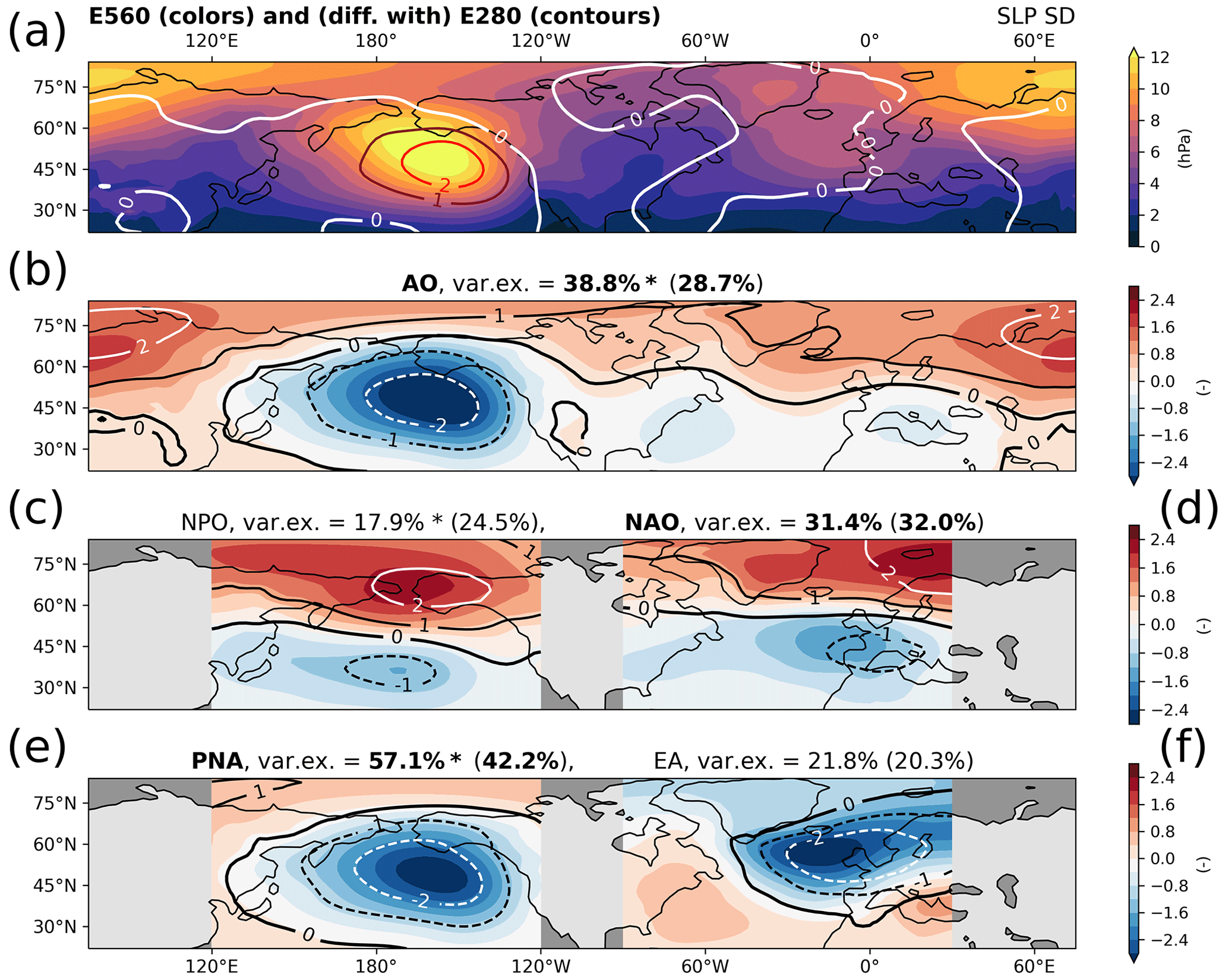
Figure 4 (a) January SLP standard deviation (SD) in CO₂ doubling (E⁵⁶⁰; colors) and difference with the pre-industrial reference simulation (E⁵⁶⁰ − E²⁸⁰; contours). (b–e) January SLP EOFs; (b) Arctic Oscillation (AO), (c) North Pacific Oscillation (NPO), (d) North Atlantic Oscillation (NAO), (e) Pacific–North American (PNA) and (f) East Atlantic (EA) patterns, with E⁵⁶⁰ in colors and E²⁸⁰ reference in contours. The leading mode in each sector is in bold. Percentage variance explained by each E⁵⁶⁰ EOF indicated (E²⁸⁰ in brackets); the asterisk (^*) indicates a statistically significant difference between these.

The spatial pattern and regional amplitude of all of the modes of variability are very similar in the E⁵⁶⁰ and E²⁸⁰ (Fig. 4b–f). As in the pre-industrial reference simulation, the leading mode in the Pacific (Atlantic) is the PNA (NAO) mode. In the AO, the amplitude of the North Pacific center of action is slightly increased, while the amplitude of the North Atlantic–Siberian center of action is reduced. The AO explains more of the total SLP variance in the CO₂ doubling (38.9 %) compared to the pre-industrial reference simulation (28.7 %), which is a statistically significant difference. Both results are consistent with the fact that there is simply more SLP variance over the North Pacific (variance defined as the square of the SLP SD, Fig. 4a).

The two leading modes in the NP explain more SLP variance in the CO₂ doubling simulation compared to the pre-industrial reference simulation (75.2 % over 66.7 %, Fig. 4c and e). This is mainly because the leading PNA mode becomes more dominant, explaining 57.2 % of the total SLP variance in this region, which is more compared to the E²⁸⁰ (42.2 %, significant difference). The second leading mode, the NPO, explains less of the total SLP variance (also significant difference). These results are consistent with those of Chen et al. (2018) that show a strengthening of PNA intensity under a strong future warming scenario in an ensemble of 35 CMIP5 models. The two leading modes in the NA are shown in Fig. 4d and f, and the percentage of variance explained remains the same in the E²⁸⁰ and E⁵⁶⁰ (no significant difference). The dipole shape of the NAO is shifted slightly polewards, and the southern node is shifted slightly westward. For the EA, the separation between positive and negative amplitude (or red and blue) moves over the Canadian archipelago in the E⁵⁶⁰, while it moves eastward and poleward from the southern tip of Greenland in the E²⁸⁰.

3.2.2 Variability in response to mid-Pliocene boundary conditions

Figure 5a shows the Eoi²⁸⁰ SLP SD and SLP SD difference with E²⁸⁰ in contours. In general, there is a decrease in SLP SD in the mid-Pliocene simulation. However, there is a substantial decrease in SLP SD over the northeastern North Pacific (up to −40 %), while there is a small increase in SLP SD over the Canadian Arctic. Furthermore, there is a decrease in SLP SD over the Scandinavian Arctic and eastern Siberia. No substantial changes are observed over the Atlantic. The changes in SLP SD in the Eoi²⁸⁰ are very similar to the SLP SD changes in the Eoi⁴⁰⁰ (see Fig. S2).

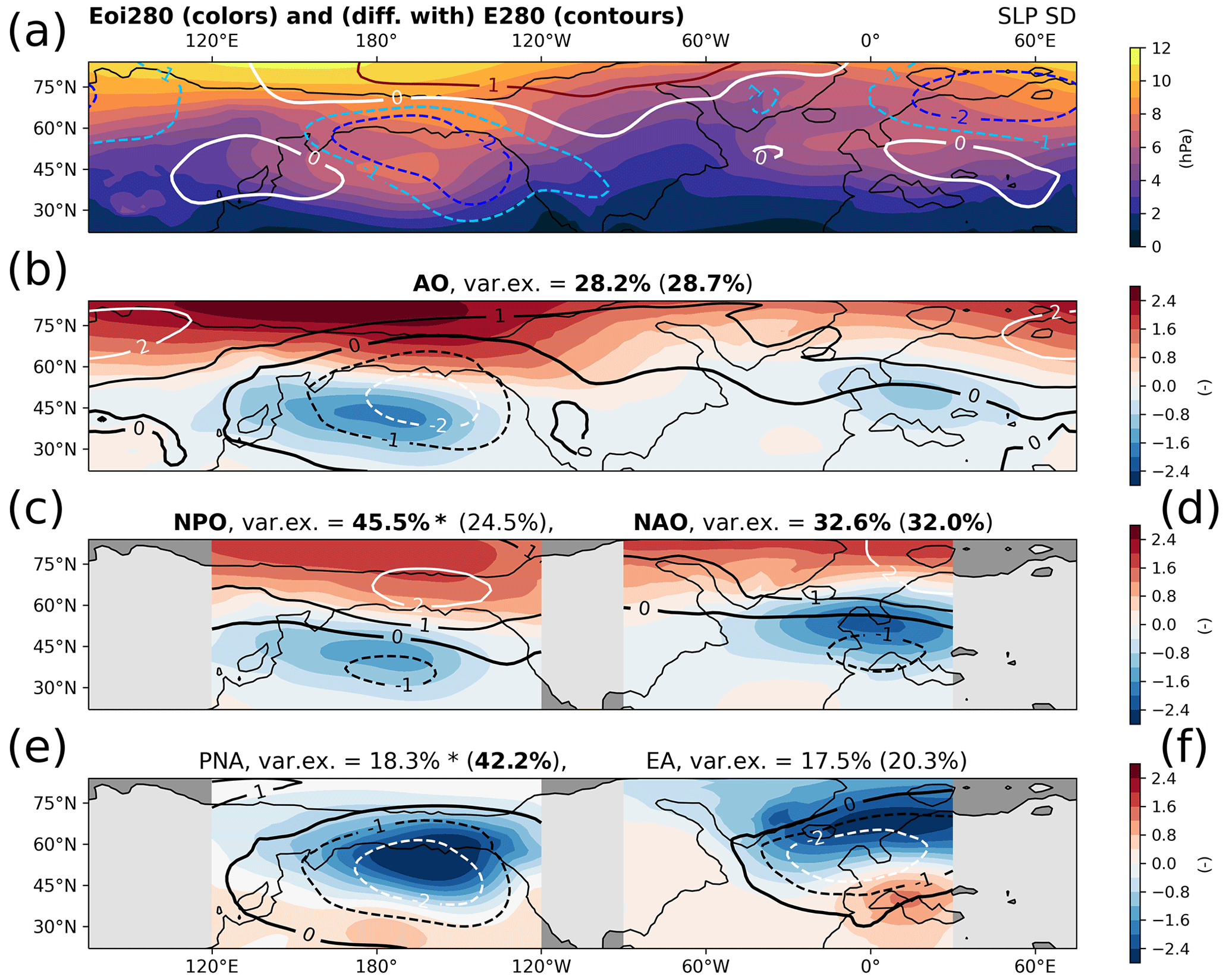
Figure 5 (a) January SLP standard deviation (SD) in mid-Pliocene boundary conditions (Eoi²⁸⁰; colors) and difference with the pre-industrial reference simulation (Eoi²⁸⁰ − E²⁸⁰; contours). (b–e) January SLP EOFs; (b) Arctic Oscillation (AO), (c) North Pacific Oscillation (NPO), (d) North Atlantic Oscillation (NAO), (e) Pacific–North American (PNA) and (f) East Atlantic (EA) patterns, with Eoi²⁸⁰ in colors and E²⁸⁰ reference in contours. The leading mode in each sector is in bold. Percentage variance explained by each Eoi²⁸⁰ EOF indicated (E²⁸⁰ in brackets); the asterisk (^*) indicates a statistically significant difference between these.

The spatial patterns of the modes of SLP variability are similar for the Eoi²⁸⁰ and E²⁸⁰ (Fig. 5b–f). Still, some distinct differences can be seen. The leading mode in the NA is still the NAO, but the leading mode in the NP becomes the NPO, whereas it is the PNA in the E²⁸⁰ and E⁵⁶⁰. The spatial pattern of the AO over the North Pacific changes quite drastically, describing more of a dipole rather than a large single center of action. The AO mode thus becomes more zonal or annular. The percentage of SLP variance explained is similar in the Eoi²⁸⁰ (28.3 %) compared to the E²⁸⁰ (28.7 %, no significant difference).

The two leading modes in the NP together explain slightly less of the total SLP variance in comparison to the pre-industrial reference simulation (63.9 % over 66.7 %, Fig. 5c and e). The leading mode becomes the NPO, explaining almost double the variance that it explains in the E²⁸⁰ (45.5 % over 24.5 %, significant difference). The spatial pattern is very similar, with notable differences being that the whole dipole is shifted slightly polewards and that both centers of action are more spread out spatially, thus representing SLP variations over a larger area. The second leading mode in the NP becomes the PNA, explaining only 18.4 % of the SLP variance compared to 42.2 % in the pre-industrial reference simulation (significant difference). The spatial extent of the monopole is slightly shifted polewards, and the region with largest amplitude extents more over the northwestern North American continent. The dominance of the NPO over the PNA is consistent with the change in SLP variance (or squared SLP SD) over this region (Fig. 5a).

The leading mode in the NA is the NAO (Fig. 5d) and explains almost the same amount of SLP variance (32.7 % over 32.2 %, no significant difference). The centers of action of the dipole are shifted slightly polewards. In particular, the southern node is more centered over northwestern European mainland, while the northern node is weakened and shifted polewards. The EA pattern (Fig. 5f) explains slightly less variance in the Eoi²⁸⁰ (17.5 % over 20.3 %, no significant difference). The center of action is shifted polewards and spread out further towards the northeast. The southern separation between negative and positive amplitude is shifted northwards over the European mainland. Over the western part of the sector, the mode resembles a dipole with a strong northern node and weak southern node.

3.2.3 Correlations between modes

Figure 6a presents the PC correlation matrix for the E²⁸⁰ as well as the CR20 reanalysis. The correlations are very similar in both cases, as can be observed from the high level of symmetry with respect to the diagonal. Both show a strong correlation between the AO and NAO and between the AO and PNA. However, in the CR20 reanalysis these two correlations are of similar magnitude, while the E²⁸⁰ shows a much stronger correlation of the AO with the PNA than with the NAO. This is consistent with the lower (higher) SLP variance over the North Atlantic (North Pacific) in the E²⁸⁰ compared to the CR20 as shown in Fig. 1b. The strongest correlation between basins is between the PNA and NAO, which can be expected since both are strongly correlated with the AO. The NPO does not correlate strongly with any other mode in both the E²⁸⁰ (only a weak correlation with the AO) and CR20.

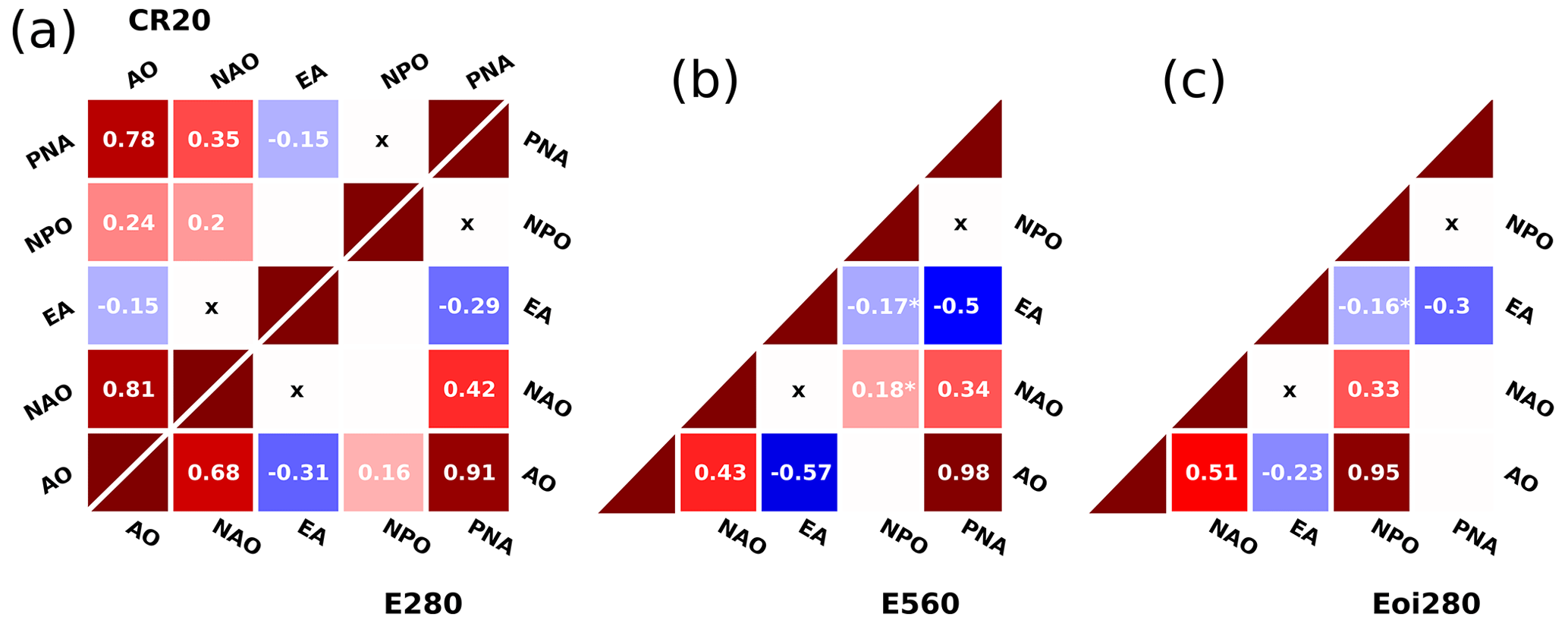
Figure 6 Correlation coefficients between principal components (PCs) time series belonging to the AO, NAO, EA, NPO and PNA modes. CR20 (a, top left), E²⁸⁰ (a, bottom right), E⁵⁶⁰ (b) and Eoi²⁸⁰ (c). Correlation coefficients are statistically significant at p<0.05 when followed by an asterisk (^*) and at p<0.005 otherwise. No correlation shown (white) when p>0.05. The × symbol represents orthogonal constructed modes (correlation 0 by definition).

The correlation matrix for the E⁵⁶⁰ shown in Fig. 6b shows great similarities with the E²⁸⁰. However, a notable difference is the even stronger correlation between the AO and PNA, of 0.98, which is consistent with the increase in SLP variance explained by the PNA in the E⁵⁶⁰ (see Fig. 4e). Interestingly, the correlation between the AO and EA is stronger than the correlation between the AO and NAO, which is not very obvious based on the similarities of the spatial patterns of these modes. The AO shows the strongest correlation with the EA (PNA) in the NA (NP), and simultaneously the EA and PNA show a stronger correlation compared to the E²⁸⁰. Again, the NPO does not strongly correlate with another mode.

The Eoi²⁸⁰ correlation matrix shown in Fig. 6c shows some notable differences with respect to the E²⁸⁰ and E⁵⁶⁰. The correlation between the AO and PNA becomes statistically insignificant. The correlation between the AO and NPO is 0.96 in the Eoi²⁸⁰, while being very small or insignificant in the other simulations. The AO shows the strongest correlation with the NAO (in the NA) and NPO (in the NP), agreeing with the earlier result that it represents a more annular mode. There is not a very strong correlation between the NPO and NAO, however, as well as between the EA and PNA. In the Eoi²⁸⁰, the PNA becomes the mode that does not correlate strongly with any other mode (except a small but significant anti-correlation with the EA).

3.3 North Pacific variability and the jet stream in response to mid-Pliocene boundary conditions

In this section, we focus on the Eoi²⁸⁰ and E²⁸⁰ results and investigate the impact of the changes in SLP variability on the jet stream in the North Pacific.

3.3.1 SLP variability and jet variations in the central North Pacific

The temporal behavior of the E²⁸⁰ and Eoi²⁸⁰ central North Pacific jet stream is shown in Fig. 7a and b, by means of a Hovmöller diagram of the zonal mean zonal wind at 200 hPa averaged over 160–220° E. The E²⁸⁰ shows a strong and focused jet with little latitudinal variations. On the other hand, the Eoi²⁸⁰ shows a generally weaker jet with a great latitudinal variation.

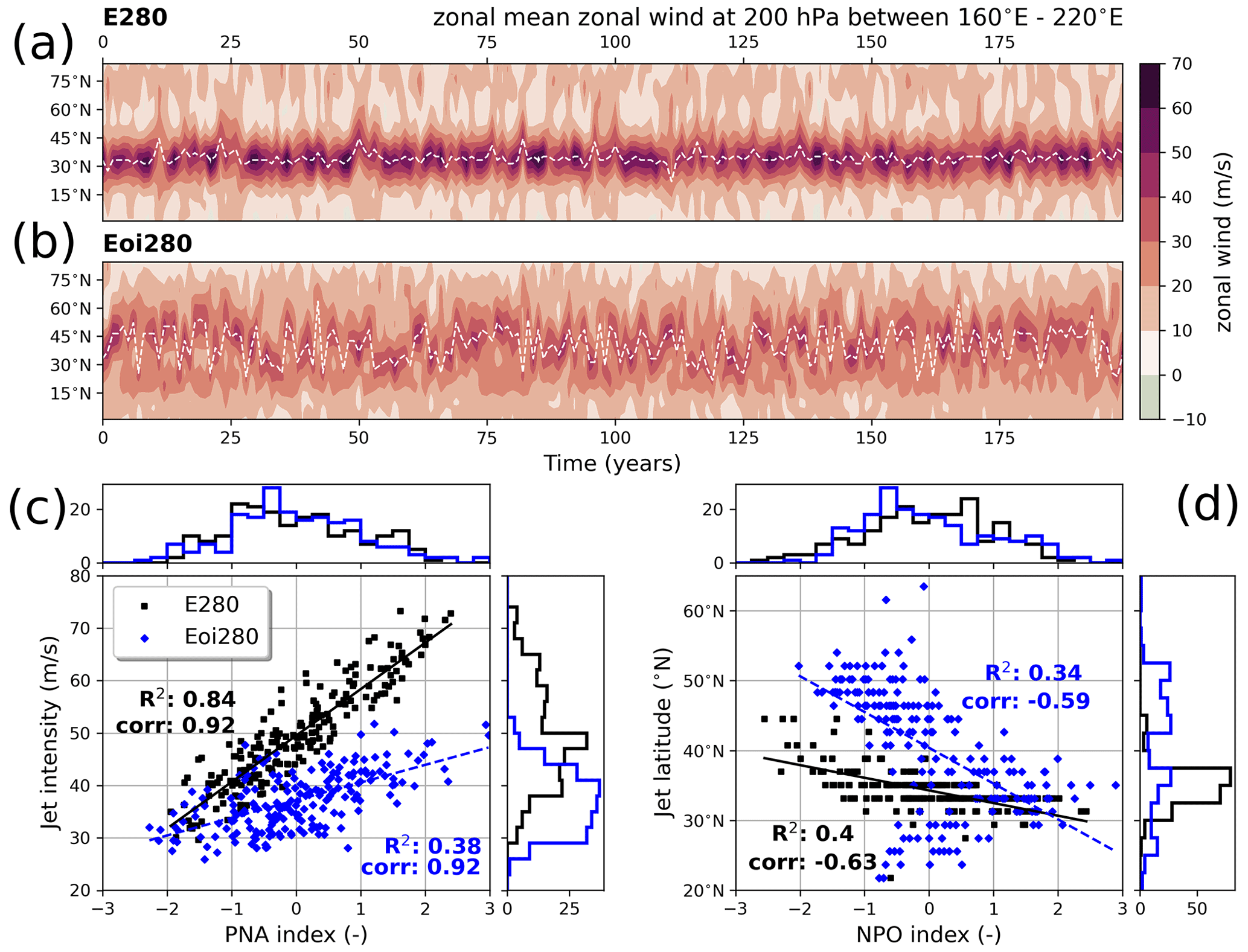
Figure 7 (a, b) Hovmöller diagrams showing zonal mean zonal wind at 200 hPa in the 160–220° E mean for every January for the E²⁸⁰ (a) and Eoi²⁸⁰ (b). The white dashed line follows the maximum of zonal wind. (c) Scatter plot including histograms of counts for the PNA index (i.e., principal component) versus the jet intensity (defined as max zonal wind). R² of linear fit and correlation coefficient are shown. E²⁸⁰ (black squares) and Eoi²⁸⁰ (blue diamonds). (d) Same but for NPO index versus jet latitude (defined at latitude of max zonal wind).

The jet intensity versus the PNA index (defined as the PC of the EOF) and the jet latitude versus the NPO index are shown in Fig. 7c and d, respectively. Figure 7c shows that the E²⁸⁰ jet intensity correlates strongly (0.92) and significantly with the PNA index. Interestingly, the Eoi²⁸⁰ jet shows the same strong (0.92) and significant correlation, but with a distribution of much lower wind speeds and much smaller R². This means that in both simulations, the jet intensity is linked to the phase of the PNA.

Figure 7d shows the relation between the jet latitude and the NPO index. In both simulations, a clear anti-correlation between the jet latitude and the NPO index is apparent. In the E²⁸⁰, the jet is located between 30–40° N. In the Eoi²⁸⁰, the jet latitude covers a much larger range, and the histogram reveals a less unimodal distribution, with two weak peaks at 30–40 and 45–55° N. The scatter plot shows that in negative NPO phases, in most years the max zonal wind is found at higher latitudes, but in some Januaries the jet latitude is found between 20–30° N. It suggests the existence of a state with two jets, where generally the northbound jet is stronger. The histogram of NPO index values furthermore shows a negative skew, coinciding with this split jet or more northward jet in the Eoi²⁸⁰. The E²⁸⁰ distribution is slightly skewed towards positive NPO values, which implies a focused jet in the subtropics. The fact that a split jet exists in the NPO− phase implies that the distribution of jet latitudes is not linear, which suggests that a linear fit might not be the best metric to capture the correlation.

The temporal behavior of the jet and the correlation between the PNA and jet intensity and between the NPO and jet latitude suggest the following. In the E²⁸⁰, the jet is mainly controlled by the PNA, with a high variation in jet intensity but not in latitude, while in the Eoi²⁸⁰, the jet is mainly controlled by the NPO, with a high variation in the jet latitude and a tendency towards a strong northwards and weak southward jet, with less variation in jet intensity. Our findings agree with the literature, where the PNA is connected to jet enhancement and displacement in the east–west direction, while the NPO is more connected to the displacement of the jet in the north–south direction (see, e.g.,  Linkin and Nigam, 2008). The dominance of the PNA (NPO) in the E²⁸⁰ (Eoi²⁸⁰) corroborates our previous findings on the percentage of SLP variance explained by both modes (see Fig. 5). Analyses using the global zonal mean zonal wind and the AO mode (Fig. S3), as well as with the PNA and jet latitude and NPO with jet intensity (Fig. S4), are included in the Supplement.

3.3.2 The phases of the mid-Pliocene NPO

The state of the NP jet stream in the NPO+ and NPO− phases in the E²⁸⁰ and Eoi²⁸⁰ is shown in Fig. 8, where the NPO+ and NPO− phases are defined as the 10 average Januaries corresponding to the 10 highest and 10 lowest NPO index values, respectively. Figure 8 shows the zonal wind and 2 PVU contour at 200 hPa on the right and the zonal mean between 160–220° E on the left for both phases and the two simulations. The E²⁸⁰ NPO− phase in Fig. 8a shows a strong jet around 30° N that deflects southward, with a sharp 2 PVU gradient along the jet core in the vertical in the central North Pacific. The E²⁸⁰ NPO+ phase shown in Fig. 8b shows a slightly weaker jet between 35–45° N, agreeing with a 2 PVU gradient that is less sharp, that moves more northward over the North Pacific.

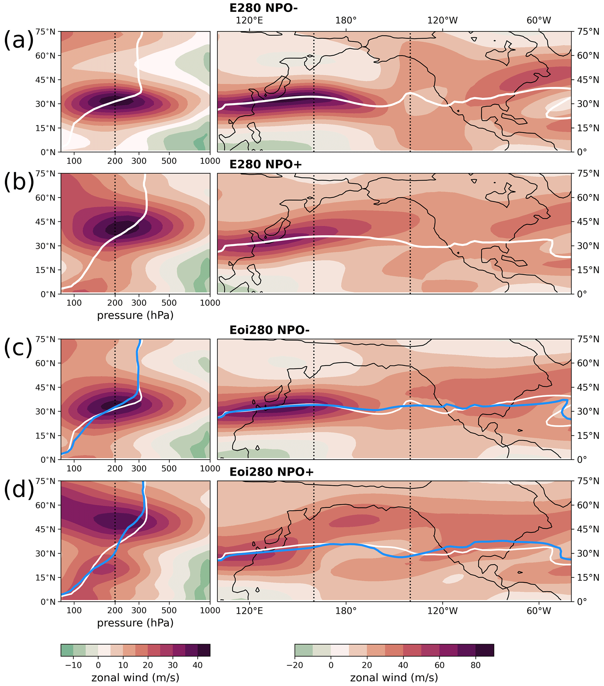
Figure 8 Zonal mean zonal wind between 160–220° E (left) and zonal wind at 200 hPa (right). E²⁸⁰ (a, b) and Eoi²⁸⁰ (c, d), representing the NPO− phases (a, c) and NPO+ phases (b, d). The contour line indicates the 2 PVU contour in white for the E²⁸⁰ (repeated in c, d) and blue for Eoi²⁸⁰. Note that the color bar range is slightly different for the left and right panels.

The Eoi²⁸⁰ NPO− phase is shown in Fig. 8c and shows similar zonal wind patterns and 2 PVU contours as in the E²⁸⁰ but at lower zonal winds (max 43.0 m s⁻¹ in the central North Pacific zonal mean over 48.2 m s⁻¹ in the E²⁸⁰). The NPO+ phase in the Eoi²⁸⁰ (Fig. 8d) is different from the E²⁸⁰, clearly showing the existence of two jets over the NP, both on the 200 hPa isobar and in the vertical cross section. The northern jet (40.2 m s⁻¹, between 45–55° N) is stronger than the southern jet (27.2 m s⁻¹, between 15–25° N), confirming the suggestion of the existence of two jets based on the results in Fig. 7d. The southern jet is located at lower pressures (or higher in the atmosphere) than the northern jet, although both jet cores follow the sharpest gradients of the 2 PVU curve. The existence of this split jet over the NP indicates a higher level of anticyclonic wave breaking on the northward side of the mean subtropical jet in comparison to the E²⁸⁰, effectively deflecting the jet towards higher latitudes. The relationship between the NPO and Rossby wave breaking is described in more detail in Rivière (2010). The fact that in all cases the strongest jets are present where the meridional PV gradient is the strongest (see Fig. 8 left panels) may indicate that the atmosphere is approximately in thermal wind balance in the January monthly mean. The nearly constant 2 PVU height over latitude between the two jets in the Eoi²⁸⁰ NPO+ (Fig. 8d, blue line) furthermore indicates a high level of meridional mixing in the atmosphere between these two jets. The SLP and SAT anomalies associated with the NPO− and NPO+ phases are shown in Fig. S5.

3.3.3 Tropical Pacific convection as an explanation

In this section, we present a hypothesis that could explain the substantial reduction in NP SLP variability under mid-Pliocene boundary conditions (Eoi²⁸⁰) and the subsequent relative dominance of the NPO and more pronounced north–south displacement of the NP jet stream. The dynamical explanation is as follows: in the Pacific sector, a weakening of the tropical convection signal (related to shifts in the mean state and due to reduced ENSO variability) leads to reduced upper-tropospheric Rossby wave activity in the extratropics, which ultimately leads to a jet stream that is weaker and less variable in east–west extent, which in turn explains the reduced variance of SLP at the surface. We highlight the steps of this mechanism in more detail below.

• 1a.

  Shifts in the tropical mean state reduce mean precipitation in the west-equatorial Pacific (WEP), specifically the westward shift of the upward branch of the Walker circulation, as well as the northward shift of the ITCZ (Fig. 3c).

• 1b.

  Reduced ENSO variability reduces WEP precipitation variability (Fig. 9a, explained in more detail below). Taking precipitation as a proxy for latent heating or convection in the tropics, both (1a) and (1b) lead to a reduced convection signal in the WEP.

• 2.

  Reduced convection in the WEP substantially weakens Rossby wave activity in the upper troposphere in the northern extratropics, primarily over the East Asia jet exit and western North Pacific (more detail below).

• 3a.

  Since the jet stream acts as a wave guide for Rossby waves (e.g.,  Branstator, 2002), reduced upper-tropospheric Rossby wave activity over East Asia leads to a North Pacific jet stream that is weaker (Fig. 2c) and less variable in strength (Fig. 7c).

• 3b.

  A weaker jet stream is associated with Rossby wave breaking downstream (e.g.,  Woollings, 2010; De Vries et al., 2013), which leads to a jet more variable in latitudinal location (e.g.,  Rivière et al., 2010) over the central and eastern North Pacific (Fig. 7d).

• 4a.

  A weak jet correlates with the negative phase of the PNA (Fig. 7c), which implies a positive SLP anomaly over the North Pacific and agrees with the MSLP difference in Fig. 2c.

• 4b.

  A jet less variable in strength implies a relatively weaker PNA, while a jet more variable in latitudinal location implies a relatively stronger NPO (according to the correlations in Fig. 7c and d), which agrees with our findings in terms of SLP variability in Fig. 5c and e.

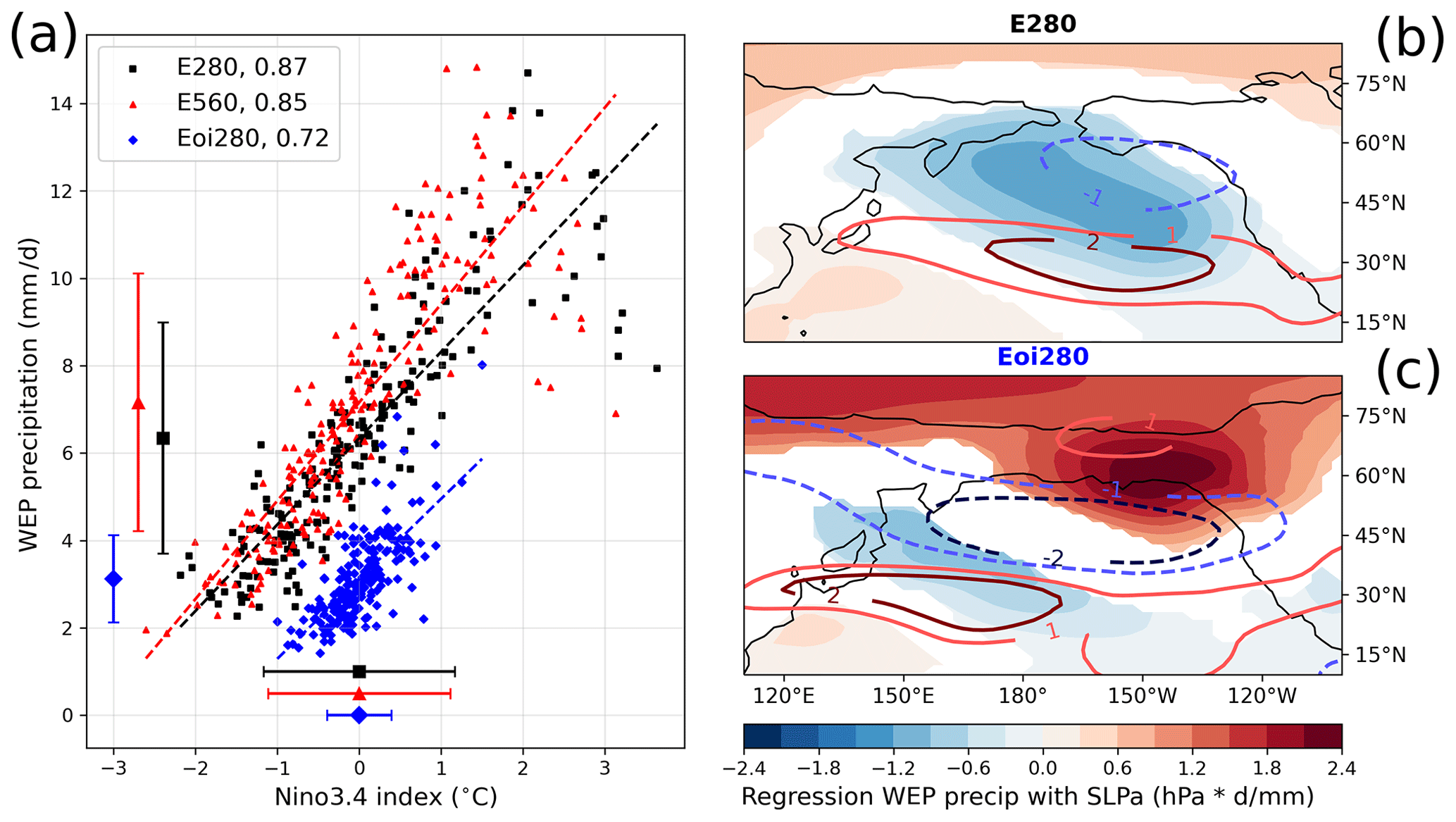
Figure 9 (a) Scatter plot of the Nino3.4 index versus average precipitation in the west-equatorial Pacific (WEP precip) for E²⁸⁰ (black squares), E⁵⁶⁰ (red triangles) and Eoi²⁸⁰ (blue diamonds), including linear regression, correlation coefficient in the legend, and mean and standard deviation values indicated range along the axes. (b, c) Regression (linear slope) between WEP precipitation and SLP anomalies (colors) and WEP precipitation and zonal wind at 200 hPa (contours) for E²⁸⁰ (b) and Eoi²⁸⁰ (c). Regression only shown when correlation is significant (p<0.05).

Figure 9a shows a scatter plot of the precipitation in the WEP as a function of the Nino3.4 index. In all of our simulations, the correlation between these two quantities is strong (>0.72), positive and statistically significant. We found that the precipitation in the WEP showed the strongest regression of the Nino3.4 index with global precipitation (see Fig. S6). The mechanism linking ENSO variability to convection in the WEP has been established (see, e.g.,  Hoskins and Karoly, 1981), so it is not surprising that the regression (or linear slope) between the two is similar for all simulations. Apart from the mean precipitation signal being lower in the Eoi²⁸⁰ (1a), the precipitation variability is also reduced (1b), which is caused by the reduction in ENSO variability. The SD of the Nino3.4 index (also called the ENSO amplitude) is reduced substantially in response to the mid-Pliocene boundary conditions (0.4 °C in the Eoi²⁸⁰; 1.1 °C in the Eoi²⁸⁰) but does not change in response to CO₂ doubling (1.1 °C in the E⁵⁶⁰). A similar reduction is observed in the Eoi⁴⁰⁰ simulation (0.4 °C).

The influence of ENSO variability on North Pacific atmospheric variability (specifically the PNA) has been described before (see, e.g.,  Mo and Livezey, 1986; Yeh et al., 2018; Domeisen et al., 2019). In short, the mechanism in the present-day climate is as follows: tropical Pacific SST anomalies lead to anomalous convection and with that force anomalies in the Hadley circulation (Hoskins and Karoly, 1981); this anomalous vertical motion leads to upper-tropospheric divergence in the tropics and convergence in the subtropics, which in turn results in vorticity anomalies (Mo and Livezey, 1986); this upper-level vorticity is a source of Rossby wave activity over the North Pacific (Mo and Livezey, 1986; Nie et al., 2019). In summary, Rossby waves connect the tropical heating signal to the atmospheric variability in the higher latitudes and thus connect ENSO variability to NP SLP variability. This connection is shown in Fig. 9b, which shows the regression (linear slope) between the WEP precipitation and the SLP (colors) and U₂₀₀ (contours) anomalies (summarizing steps 2–4b of the mechanism). The results show that the E²⁸⁰ simulation is able to capture the connection between tropical convection and North Pacific SLP and jet stream variations. This mechanism breaks down in the Eoi²⁸⁰ (Fig. 9c). The regression pattern of WEP precipitation with SLP shows more of a dipole (reminiscent of the NPO pattern), and the regression pattern of WEP precipitation with the jet variability moves such that it represents more latitudinal variation in the jet stream. Note that while the regression has similar, or stronger, values in the Eoi²⁸⁰ compared to E²⁸⁰, the WEP precipitation values are substantially lower and thus lead to lower values for SLP and U₂₀₀ variations as well. More analysis on the connection between tropical convection and Rossby wave activity, including a computation of the Rossby wave source, can be found in Sect. S5 and Figs. S7–S9 in the Supplement.

4 Discussion

4.1 Physical and dynamical interpretation

4.1.1 Changes in variability and changes in the winter mean state

Under CO₂ doubling, our simulations show a strengthened PNA, consistent with a general increase in SLP SD over the North Pacific. This is consistent with a study by Chen et al. (2018) that shows a strengthening of PNA intensity under a strong future warming scenario in an ensemble of 35 CMIP5 models. They link it to a strengthening of tropical Pacific precipitation response, caused by enhanced central equatorial Pacific SST variability. Our E⁵⁶⁰ simulation does show a slight enhancement of tropical Pacific precipitation (see Figs. 3b and 9a). Furthermore, we find a slight intensification of the NP subtropical jet stream (Fig. 2b), which according to the relationship described in Fig. 7c is related to an enhanced PNA.

As a response to mid-Pliocene boundary conditions, we find a relative strengthening of the NPO and simultaneous weakening of the PNA, with a general decrease in SLP SD over the North Pacific. The NPO becomes dominant even on a hemispheric scale where it correlates strongly and significantly with the AO. The North Pacific jet becomes weaker (consistent with other PlioMIP2 studies; Hunter et al., 2019; Menemenlis et al., 2021; Feng et al., 2022) and more variable in latitude, which is correlated with NPO variability. The North Pacific winter climate is oscillating between states either with a relatively strong jet (NPO−) or with a split jet that has a strong northward jet and weak southward jet (NPO+). In the winter mean, there is a strong increase in MSLP over the North Pacific, weakening the Aleutian low (consistent with Menemenlis et al., 2021). In the previous section, we have described a hypothesis by which changes in the tropical Pacific could explain the changes in North Pacific atmospheric variability due to mid-Pliocene boundary conditions.

To summarize, in both simulations, the changes in NH atmospheric variability are mainly related to changes in the tropical Pacific mean state. In response to CO₂ doubling, the changes in this mean state are small, as are changes to the NP variability. In response to mid-Pliocene boundary conditions, the changes in the tropical mean state are substantial, leading to large changes in the variability of the jet stream and the SLP patterns. The changes in the NA mean state, as well as in NA variability, are small.

4.1.2 The role of mean surface temperature response

Qualitatively, the SAT response to increased CO₂ and to the mid-Pliocene BCs is similar. However, an energy budget analysis reveals that the radiative forcings leading to the warming are not the same. We diagnose surface temperatures with shortwave and longwave radiation, using a simple model assuming a gray atmosphere without turbulent heat fluxes (following Heinemann et al. (2009) and Baatsen et al. (2022), results shown in Fig. S10). The surface warming in the E⁵⁶⁰ is explained by changes in effective emissivity from the increased greenhouse gas concentrations. The surface temperature response in the Eoi²⁸⁰ is a combination of changes in planetary albedo, as well as effective emissivity. The changes in emissivity here are related to lapse rate feedbacks and changes in water vapor. The warming due to changes in planetary albedo is mostly related to changes in vegetation and lakes. Albedo changes from the reduced Greenland Ice Sheet do not contribute to warming in January because the incoming solar radiation is at a minimum. This is different in the annual mean, as seen in Baatsen et al. (2022). In both simulations, warming in areas with sea-ice loss is related to changes in emissivity from increased evaporation leading to increased cloud cover.

Menemenlis et al. (2021) find a similar SAT response in their mid-Pliocene simulations with CCSM4-UoT to our Eoi²⁸⁰ response in Fig. 3c and interpret it as a cool phase of the PDO, which is related to a weakened Aleutian low. While the connection between the PDO and Aleutian low is clear from literature (see, e.g.,  Hurwitz et al., 2012; Simon et al., 2022), assessing the links with (multi)decadal variability is outside of the scope of this work, and Pacific (multi)decadal variability in the PlioMIP2 ensemble will be investigated in future research. We interpret the weakening of the Aleutian low in our Eoi²⁸⁰ simulation as a weakening of the dominance of the PNA in the pre-industrial reference simulation, which simultaneously allows the NPO to exert more influence on the North Pacific winter climate. As Linkin and Nigam (2008) explain, the NPO can be considered a Pacific analogue to the NAO in the NA. In the present-day climate, the amplitude of the NAO is large and the NA jet relatively weak, while the NPO amplitude is small and the NP jet relatively strong. In our mid-Pliocene simulations, the NP jet weakens up to 50 % and the NPO becomes the dominant mode of variability in the NP. This implies that – like the NAO in the present-day NA – SLP anomalies related to NPO variability strongly relate to the latitudinal displacement of the NP jet. This is what we see in Fig. 7d. The split jet condition over the NP, related to the NPO+ phase in the mid-Pliocene simulation (Fig. 8d), is also reminiscent of the dynamic behavior of the jet in the present-day NA, corroborating the NAO analogue even further.

4.2 A climate variability point of view

How do the observed mid-Pliocene changes in North Pacific winter variability link to other modes of variability? Apart from the dominant Pacific teleconnection between canonical ENSO, PDO and PNA, the NPO has been linked to the North Pacific meridional mode (NPMM, Chiang and Vimont, 2004; Linkin and Nigam, 2008), as well as to the central Pacific ENSO, also known as El Niño Modoki or warm pool El Niño (Furtado et al., 2012; Ding et al., 2022). In Sect. 3.3.3, we show that the North Pacific SLP variability relates to ENSO variability but not specifically to which ENSO flavor nor how other modes of variability could be involved. We know that in the Eoi⁴⁰⁰ simulation with CCSM4-Utr the canonical ENSO variability is reduced (Oldeman et al., 2021), as well as the variability of the PDO (Baatsen et al., 2022, referred to as Pacific multidecadal variability or PMV). The reduced canonical ENSO and PDO variability could be connected to the reduced PNA variability in the North Pacific winter. Oldeman et al. (2021) also show a slight relative increase in the number of central Pacific ENSO events over canonical ENSO events in the CCSM4-Utr Eoi⁴⁰⁰, consistent with the relative strengthening of the NPO. However, the mid-Pliocene NPMM is shown to be substantially weaker in CCSM4-Utr compared to the pre-industrial reference simulation by (Pontes et al., 2022, extended data). Recently though, Stuecker (2018) showed that the PNA and PDO are also connected to the NPMM and central Pacific ENSO, especially on low frequencies. Our results consistently show a total reduction in the Pacific oceanic and atmospheric variability in the CCSM4-Utr mid-Pliocene simulations, with a clear reduction of the dominant teleconnection (PNA, PDO and canonical ENSO) and a relative increase in the prominence of the second leading teleconnection (NPO, NPMM and central Pacific ENSO).

4.3 Sensitivity to the mid-Pliocene boundary conditions and CO₂

In this study we have investigated mid-Pliocene NH winter variability and separated the response to either CO₂ or to mid-Pliocene boundary conditions other than CO₂. We find large differences between both climate forcings. In this section we want to discuss how sensitive the responses found are to the combination of mid-Pliocene boundary conditions and elevated CO₂. Furthermore, we explore which of the specific boundary condition changes in the Eoi²⁸⁰ could explain the observed response.

Firstly, we want to address the non-additivity of the responses to changes in boundary conditions or elevated CO₂. To investigate this, we briefly study the results of an additional Eoi⁵⁶⁰ simulation (described in  Baatsen et al., 2022), which represents a simulation with mid-Pliocene boundary conditions and a doubled pre-industrial CO₂ level. With this simulation, we can assess the response to mid-Pliocene boundary conditions at elevated CO₂ conditions (Eoi⁵⁶⁰ − E⁵⁶⁰), as well as the response to a CO₂ doubling in mid-Pliocene boundary conditions (Eoi⁵⁶⁰–Eoi²⁸⁰). The results in terms of MSLP difference and SLP SD difference are included in the Figs. S11 and S12. The MSLP difference (Fig. S11) is very consistent in response to a CO₂ doubling (i.e., no substantial change) as well as in response to mid-Pliocene boundary conditions (i.e., a substantial increase in NP MSLP), for all simulations. The SLP SD difference across the set of simulations (Fig. S12) is similar but not entirely the same. The NP SLP SD increase for the CO₂ doubling with present-day geography (E⁵⁶⁰ − E²⁸⁰) is not seen in the CO₂ doubling at mid-Pliocene boundary conditions (i.e., no substantial change; Eoi⁵⁶⁰–Eoi²⁸⁰). The NP SLP SD decrease for the mid-Pliocene boundary conditions at low CO₂ (Eoi²⁸⁰ − E²⁸⁰) is also seen at higher CO₂ (Eoi⁵⁶⁰ − E⁵⁶⁰) but slightly intensified. Finally, the response to the main mid-Pliocene simulation in PlioMIP2 (Eoi⁴⁰⁰ − E²⁸⁰) seems to be an added combination of the responses to the mid-Pliocene BCs and elevated CO₂. The reduction of NP SLP SD is seen but slightly less than in response to the Eoi²⁸⁰, which would be the scaled effect of the response to the E⁵⁶⁰. Research by Garfinkel et al. (2020) shows that the stationary wave response to various boundary conditions is not always linear and additive, however. A more in-depth analysis on the nonlinearity and nonadditivity of the winter variability response is out of the scope of this work.

Secondly, we want to hypothesize which specific change in the boundary conditions of the mid-Pliocene simulation could be mainly responsible for the observed responses. As we have not performed these sensitivity studies with our own model, we will turn to results from studies performed with other PlioMIP2 models. Some modeling groups performed simulations with either just reduced land ice cover (including the reduced GIS) or just changes to the orography, which includes the closure of gateways (including the Bering Strait and Canadian Arctic Archipelago), vegetation changes, and minor topography and bathymetry changes. Stepanek et al. (2020) perform these sensitivity studies with climate model COSMOS and find that the annual mean climate response (in terms of surface temperatures and precipitation) is generally more sensitive to the changes in orography compared to changes in ice sheets. Specifically in terms of tropical Pacific precipitation, the response to orography is substantial (albeit not the same as for our Eoi²⁸⁰ simulation), while the response to reduced ice sheets is insignificant (compared to the E²⁸⁰). Employing sensitivity studies with climate model CCSM4-UoT, Chandan and Peltier (2018) show that the northern-higher-latitude climate (in terms of annual mean as well as winter mean surface temperatures and sea-ice cover) is also more sensitive to changes in orography than changes in ice sheets. Also using the CCSM4-UoT simulations, Menemenlis et al. (2021) find that a wintertime stationary wave pattern present over the pre-industrial North Pacific nearly disappears in the mid-Pliocene. They show that this reduced wave train response is present in the simulations with changed orography, as well as the simulation with reduced ice sheets (in almost equal amplitude), but not in simulations with just elevated CO₂. Regarding which specific orography change could cause most of the response, Otto-Bliesner et al. (2017) uses CCSM4 simulations and finds that there is a similar response in North Pacific Arctic climate to closing just the Bering Strait or just the Canadian Arctic Archipelago. To summarize, studies with other climate models indicate a large sensitivity of the climate response to changes in orography (including the closed gateways) over the changes in ice sheet cover. However, these results do not automatically translate to the winter variability response or to our specific model used here.

4.4 A reflection on model performance

When comparing our E²⁸⁰ pre-industrial reference simulation with the CR20 reanalysis (see Fig. 1), we find some large biases with regards to the MSLP and total SLP SD. The MSLP gradient in the NA is greatly overestimated. However, the NAO and EA are well reproduced, and the main differences within the set of simulations are not in the NA. In terms of SLP SD, there is an overestimation of the variance over the NP and an underestimation over the NA, which is a known model bias (Eyring et al., 2021). This affects the AO mode, as well as the differences between the CR20 and E²⁸⁰ in terms of correlations between the different modes (Fig. 6). While the SLP SD in the NP is overestimated, the NPO and PNA are well reproduced both in terms of spatial pattern and in variance explained by each mode. We are therefore confident in our results regarding shifts in NPO and PNA in our set of simulations.

The choice to evaluate only one model was based on the fact that CCSM4-Utr has a unique set of sensitivity simulations that most other PlioMIP2 modeling groups have not performed. However, a limitation is that the results are biased towards the performance and sensitivities of CCSM4-Utr. While most PlioMIP2 modeling groups have not performed the Eoi²⁸⁰ and E⁵⁶⁰ simulations, we can still try to extrapolate the dynamical explanation based on results with the Eoi⁴⁰⁰ simulation that has been performed by all modeling groups. Most PlioMIP2 models, including CCSM4-Utr, show (1) a northward shift of the ITCZ (Pontes et al., 2022), (2) a westward expansion of the Walker circulation (Han et al., 2021) and (3) a reduction of the ENSO variability (Oldeman et al., 2021) in the mid-Pliocene Eoi⁴⁰⁰. Considering our dynamical hypothesis linking shifts in Pacific convection to the changes in SLP variability, this could indicate that we can expect similar changes to those found in CCSM4-Utr across the PlioMIP2 ensemble. However, for all of these three features, the CCSM4-Utr Eoi⁴⁰⁰ simulation is the model with the largest change in that direction, which would imply that CCSM4-Utr might be an end-member of the spectrum. An assessment of the changes in NP variability and their relation with ENSO changes in the full PlioMIP2 is planned for future research.

Haywood et al. (2020) assess climate sensitivity across the PlioMIP2 ensemble and report that CCSM4-Utr has a relatively low equilibrium climate sensitivity (ECS; 3.2 compared to 3.7 in the ensemble mean). However, it has a relatively high Earth system sensitivity (ESS; 9.1 compared to 6.2 in the ensemble mean). ECS and ESS are both measures of the climate's sensitivity to a CO₂ doubling, but ESS takes into account long-term feedbacks such as adjustment to changes in ice sheets and to changes in orography, whereas ECS just considers CO₂ sensitivity. CCSM4-Utr's high ESS but low ECS indicates a large sensitivity to the mid-Pliocene boundary conditions other than elevated CO₂. This would indicate that while the response in the Eoi²⁸⁰ simulation might largely dictate the response in the Eoi⁴⁰⁰ for CCSM4-Utr, this does not have to be the case for many of the other PlioMIP2 models.

4.5 The mid-Pliocene as a future climate analogue?

In the introduction, we posed the question of whether the mid-Pliocene can be considered as an analogue for future changes in atmospheric winter variability in the NH. In terms of temperature and precipitation, Burke et al. (2018) show that end of this century climate would be most analogous to the mid-Pliocene, both following the RCP4.5 and RCP8.5 scenarios, compared to other past warm climates. We also find that the winter SAT response to elevated CO₂ or to mid-Pliocene boundary conditions other than CO₂ are similar. However, we find that the response in winter SLP variability is almost opposite to both forcings, especially over the North Pacific. This is similar for the mid-Pliocene ENSO and AMOC, where the changes are also opposite to end-of-the-century projections (Pontes et al., 2022; Weiffenbach et al., 2023). This could already disqualify the mid-Pliocene as a future analogue for these climate features, but one could argue that some mid-Pliocene boundary conditions are actually long-term Earth system feedbacks to elevated atmospheric CO₂, such as the changes in ice sheets and vegetation (Feng et al., 2022). However, following the sensitivity study results in Chandan and Peltier (2018), it seems that the biggest influence on mid-Pliocene higher-latitude climate is changes in orography, which includes the closed Arctic gateways, rather than the reduced Greenland Ice Sheet or elevated CO₂. The Bering Strait is not expected to close in the coming centuries or millennia, so this disqualifies the mid-Pliocene as an analogue for a future warm climate. However, the analysis in this paper is restricted explicitly to the NH winter. Other seasons and regions in the mid-Pliocene climate may behave differently and potentially more analogous to what is expected for increased future CO₂ levels. Furthermore, other models might be less sensitive to the mid-Pliocene boundary conditions and could be better candidates to assess a future climate analogy.

5 Summary and conclusions

In this study, we address the question of whether the mid-Pliocene climate can be used to investigate the response of NH winter atmospheric variability, such as the NAO, NAM and PNA, to increased CO₂. To answer that question, we want to know (1) whether there is a difference in the response to elevated CO₂ and to mid-Pliocene boundary conditions other than CO₂, including closed Arctic gateways and reduced ice sheets, and (2) how changes in mean winter climate relate to changes in atmospheric variability in the NH. We use a version of the CESM1.0.5 that is a part of PlioMIP2, and we show that the pre-industrial reference simulation is good at reproducing patterns of SLP variability when compared to the CR20 reanalysis. We use a set of sensitivity simulations to separate the response to a CO₂ doubling and the response to mid-Pliocene boundary conditions other than CO₂.

Considering subquestion (1), we find that although winter surface temperatures respond in a similar way to CO₂ or to mid-Pliocene boundary conditions, the responses in mean SLP, jet stream and precipitation show distinct differences. In the CO₂ doubling simulation, there is little response in mean SLP, while the mid-Pliocene shows a large increase in mean SLP over the North Pacific, together with a weakened jet stream. Regarding SLP variability, we find an increase in North Pacific SLP variance and a strengthening of the Pacific–North American pattern (PNA) in response to CO₂ doubling, consistent with the literature, and no notable changes over the North Atlantic. An opposite response is seen in the mid-Pliocene boundary condition simulation, where SLP variance decreases over the North Pacific, the PNA becomes weaker and the North Pacific Oscillation (NPO) becomes the dominant mode of variability. We find a strong correlation between the PNA and North Pacific jet intensity, on the one hand, and the NPO and jet latitude, on the other hand, both in pre-industrial and mid-Pliocene simulations.

Considering subquestion (2), we find that the pre-industrial climate, characterized by a strong PNA, shows a strong mean jet with variations in jet strength but not in latitude. The mid-Pliocene boundary condition simulation shows a weak mean jet that is less variable in intensity but has a high level of variation in jet latitude, consistent with a dominant NPO. We hypothesize that the weakening of the North Pacific jet stream is ultimately related to shifts in the tropical Pacific precipitation signal, both in the mean and in its variability. Both a reduced ENSO variability and shifts in the mean ITCZ position and upward branch of the Walker circulation weaken the tropical Pacific precipitation response, which in turn leads to a weaker North Pacific jet stream.

The large sensitivity of the mid-Pliocene climate to changes in boundary conditions other than elevated CO₂ leads us to conclude that the mid-Pliocene climate is not a good candidate to determine the response of NH winter atmospheric variability to increased CO₂. The opposite response in North Pacific winter variability to elevated CO₂ as opposed to mid-Pliocene boundary conditions weakens the notion of the mid-Pliocene climate as a future analogue, especially since the closure of the Arctic gateways is not a long-term Earth system feedback to elevated CO₂.

Even though we consider the CESM1.0.5 a suitable model for this study, it may be an end-member in the PlioMIP2 ensemble in terms of its winter variability response. In future research we plan to extend the investigation to the rest of the PlioMIP2 ensemble. In addition, the specific mechanisms by which the different mid-Pliocene boundary condition cause the changes in SLP variability and jet variations can be investigated in more detail. The specific response to these individual forcings, and the possible non-linear interaction between them, is an important open issue, which if resolved can help us understand how the winter climate responds to changing forcings in a warmer future.