the Creative Commons Attribution 4.0 License.
the Creative Commons Attribution 4.0 License.
 | 03 Apr 2024
A Lagrangian framework for detecting and characterizing the descent of foehn from Alpine to local scales
Lukas Papritz
Michael Sprenger
When foehn winds surmount the Alps from the south, they often abruptly and vigorously descend into the leeside valleys on the Alpine north side. Scientists have long been intrigued by the underlying cause of this pronounced descent. While mountain gravity waves and the hydraulic theory provide theoretical foundations to explain the phenomenon, the descent of the Alpine south foehn has, so far, not been explicitly quantified and characterized for a series of real-case events. To fill this research gap, the present study employs kilometer-scale numerical simulations, combined with online trajectories calculated during model integration. In an innovative approach, we adopt the Lagrangian perspective, enabling us to identify the descent and determine its key characteristics across foehn regions spanning from the Western to the Eastern Alps.
In the first part of the study, we find the descent of foehn air parcels to be primarily confined to distinct hotspots in the immediate lee of local mountain peaks and chains, underlining the fundamental role of local topography in providing a natural anchor for the descent during south foehn. Consequently, the small-scale elevation differences in the underlying terrain are clearly linked to the magnitude of the descent, whereby other contributing factors also influence the process. Combined with the fact that the descent is mostly dry adiabatic, these results suggest that the descending motion occurs along downward-sloping isentropes associated with gravity waves. A small proportion of air parcels experience diabatic cooling and moisture uptake during the descent, which predominantly occur to the south of the Alpine crest.
The second part of the study aims to elucidate the different factors affecting the descent on a local scale. To this end, a particularly prominent hotspot situated along the Rätikon, a regional mountain range adjacent to the Rhine Valley, is examined in two detailed case studies. During periods characterized by intensified descent, local peaks along the Rätikon excite gravity waves that are linked to the descent of air parcels into the northern tributaries of the Rätikon and into the Rhine Valley. The two case studies reveal that different wave regimes, including vertically propagating waves, breaking waves, and horizontally propagating lee waves, coincide with the descent. This suggests the absence of a specific wave regime that is consistently present during foehn descent periods along the Rätikon. In addition to gravity waves, other effects likewise influence the descent activity. For example, a topographic concavity deflects the near-surface flow and thus promotes strong descent of air parcels towards the floor of the Rhine Valley. In addition, in one of our cases, nocturnal cooling introduces a smooth virtual topography that inhibits the formation of pronounced gravity waves and impedes the descent of foehn air parcels into the valley atmosphere.
In summary, this study approaches a long-standing topic in foehn research from a new angle. Given the limitations of our model simulations, we did not attempt to unequivocally resolve the causes for the descent. Nevertheless, using online trajectories, we explicitly identified and characterized the descent of foehn. The innovative Lagrangian method enabled us to diagnose descent within a comprehensive dataset, encompassing multiple case studies and a wide range of different foehn regions. The findings highlight the benefits offered by the Lagrangian perspective, which not only complements but also substantially extends the previously predominant Eulerian perspective on the descent of foehn.
- Article
(20099 KB) - Full-text XML
-
Supplement
(38432 KB) - BibTeX
- EndNote


A major fraction of Earth's surface is characterized by complex terrain (Rotach et al., 2014). Downslope winds, forming in the lee of orographic obstacles, therefore constitute a ubiquitous phenomenon of mountain meteorology (e.g., Smith, 1979). While these winds are referred to as foehn in the Alps, they are given different local names in numerous regions worldwide and have already been extensively documented (e.g., Raphael, 2003; Elvidge et al., 2014; Muñoz et al., 2020; Kusaka et al., 2021). Foehn winds are well known for their typical characteristics: their onset in a valley is usually marked by an abrupt increase in temperature and a decrease in relative humidity, while the wind and gust speeds pick up markedly (e.g., Richner and Hächler, 2013; Sprenger et al., 2016).
In the Alpine region, foehn winds are known for their beneficial impacts, yet they are even more infamous for their adverse impacts. Folkloristic narratives blame the foehn for a range of negative effects on human health, such as insomnia, migraines, and general discomfort for parts of the population (e.g., Strauss, 2007). Additionally, the gale-force winds can damage buildings and forests (e.g., Stucki et al., 2015). They also pose a danger to aviation and cable car operators (Richner and Hächler, 2013) and notoriously accelerate snowmelt over mountainous regions (e.g., Streiff-Becker, 1930). Furthermore, the occurrence of south foehn has been linked to peaks in the ozone concentration in northern foehn valleys (Baumann et al., 2001; Seibert et al., 2000). In the Alps, the arguably most hazardous impact of foehn concerns its potential to create atmospheric conditions that promote the ignition and rapid spread of forest fires (Zumbrunnen et al., 2009; Wastl et al., 2013; Pezzatti et al., 2016; Mony, 2020). In the polar regions, foehn flows have been found to enhance surface melt and, for example, increase melt rates over Antarctic ice shelves (e.g., Elvidge et al., 2020; Zou et al., 2021). Similarly, foehn effects are attributed a role in surface melt over the Greenland Ice Sheet (Mattingly et al., 2020, 2023).
Owing to their fierce nature and the associated impacts, foehn winds have attracted the interest of scientists going back to the 19th century (e.g., Hann, 1866). Two key questions were posed early on (e.g., Steinacker, 2006) and heavily debated throughout: why is the foehn so extraordinarily warm when arriving in the valleys? And why does the potentially warmer foehn air descend from aloft to replace potentially colder air in the valleys? The first of these questions (i.e., the warming) has lately received a lot of attention by scientific research (e.g., Elvidge and Renfrew, 2016; Miltenberger et al., 2016; Kusaka et al., 2021; Jansing and Sprenger, 2022). Interestingly, the second question (i.e., the descent), while likewise being an archetypal feature of foehn flows, has not received the same consideration in recent work. Accordingly, this paper shifts the focus towards the descent of the foehn.
As mentioned previously, the physical cause for the descent was in the epicenter of the early scientific debates on foehn. Over the course of the 19th and the 20th centuries, a whole range of “foehn theories” was proposed. Some researchers attributed an active role to the foehn flow (e.g., Wild, 1868; Streiff-Becker, 1930), while others interpreted the foehn descent as a passive replacement flow when air is aspirated out of the valleys upon the approach of a synoptic low-pressure system (e.g., Billwiller, 1878; Ficker, 1931). With the solenoid theory, Frey (1945) proposed the first fluid-dynamical explanation of the foehn descent. However, according to Richner and Hächler (2013), it remains unclear whether the solenoid field is, in fact, an effect of the foehn rather than its cause. Rossmann (1950) and Schüepp (1952), in turn, suggested that microphysical processes in the clouds of the foehn wall could play a key role in the downward acceleration: as the cloudy air starts to descend downstream of the crest, evaporative cooling of the hydrometeors induces a negative buoyancy relative to the environment, which would result in a downward acceleration (the waterfall theory; see, e.g., Steinacker, 2006; Sprenger et al., 2016). Yet, since not all foehn events are accompanied by clouds on the Alpine south side, this hypothesis might at most explain a downward acceleration of the flow for some cases. For further details on the different foehn theories, the reader is referred to the existing literature (e.g., Lehmann, 1937; Gubser, 2006; Steinacker, 2006; Richner and Hächler, 2013; Sprenger et al., 2016).
An alternative concept to explain the dynamics of foehn was introduced by Schweitzer (1952). He used the analogy of a shallow layer of water flowing in a canal to explain foehn as a flow transitioning from a subcritical to supercritical state. During the Mesoscale Alpine Programme (MAP; Bougeault et al., 2001), the applicability of the hydraulic analogue to gap flows in the Wipp Valley was extensively investigated. Indeed, several features reminiscent of hydraulic flow, like a transition of the flow regime and hydraulic jumps, were observed and modeled during the campaign (Flamant et al., 2002; Gohm and Mayr, 2004; Armi and Mayr, 2007). With regard to the descent of the gap flow, Mayr et al. (2007) stated that “Buoyancy forces as used in hydraulics are the key mechanism behind the descent”. In other words, potentially colder air upstream of a gap will flow downwards until it reaches the level of neutral buoyancy. Accordingly, Mayr and Armi (2008) argue that potential temperature differences between upstream and downstream air masses are the prerequisite for a cross-barrier flow to descend and form a foehn. However, if the leeside valley air has a lower potential temperature compared to the overflowing air, the descending flow separates from the slope and traverses the virtual topography formed by the colder air mass beneath. Consequently, this virtual topography, rather than the real topography, controls the descending flow (Armi and Mayr, 2015). The temperature difference between upstream and downstream air can be modulated by local processes (e.g., nocturnal cooling) or arises from larger-scale advection of colder air. Past studies have applied the conceptual model of hydraulics to explain the dynamics of both shallow foehn and deep foehn (e.g., Armi and Mayr, 2007, 2015).
Largely separate from the abovementioned foehn theories, mountain gravity waves were discovered and studied using theory, observations, and later on also numerical models (e.g., Blumen, 1990). Queney (1948) was among the first to apply gravity wave theory to explain the strong acceleration of downslope winds. Essentially, the downslope motion in the lee of a mountain can be interpreted as an adiabatic descent along deflected isentropes. This deflection is an essential feature of mountain gravity waves. The amplitude of gravity waves is determined by the upstream atmospheric profile, the shape of the obstacle, and the downstream conditions. Researchers have found two theories of how gravity waves potentially amplify downslope flows. On the one hand, Klemp and Lilly (1975) suggested an amplification process based on the partial internal reflection and constructive superposition of propagating gravity waves, inducing strong surface winds downstream of the obstacle. On the other hand, it was found that, under certain conditions, gravity waves can become convectively unstable, which is commonly referred to as wave breaking (e.g., Durran, 1990). The breaking region then acts as an internal reflector (i.e., a critical level) on upward-propagating gravity waves (Clark and Peltier, 1977). Consequently, a strong surface response in the form of a downslope windstorm emerges within the resonant cavity. Elvidge et al. (2020) thus concluded that foehn “is an intrinsic feature of mountain gravity waves”.
During MAP, the role of gravity waves in the foehn flow in the Rhine Valley and the Wipp Valley was also investigated. In the Rhine Valley, strong downward motion and a modulation of the near-surface flow by the gravity waves aloft were diagnosed during intensive observation period (IOP) 12 (Drobinski et al., 2003). During IOP 10, the gravity waves excited by the surrounding topography propagated into the region of the valley axis, and their amplification concurred with striking maxima in the low-level wind field near Vaduz (Zängl et al., 2004a). An analogous acceleration of low-level winds due to large-amplitude gravity waves has been reported for the Wipp Valley using idealized (Zängl, 2003) and real-case simulations (Gohm et al., 2004; Zängl et al., 2004b). Interestingly, a further case study of a south-foehn event indicated that trapped lee waves might also be related to the occurrence of severe near-surface winds (Zängl and Hornsteiner, 2007). In this case, the descending motion would be associated with downward-sloping isentropes on the upstream side of the wave troughs. In essence, the MAP findings highlighted the vital importance of mountain waves for the mesoscale and small-scale characteristics and the evolution of the foehn flow (Drobinski et al., 2007).
However, in order for the foehn flow to actually penetrate down to the surface of the valleys, the frequently present cold-air pools within Alpine valleys need to be eroded as well. The literature presents three mechanisms that potentially support the erosion of preceding cold-air pools, namely bottom-up erosion by solar radiation and associated surface sensible heat fluxes; top-down erosion by shear-induced turbulence; or displacement of the cold-air pool, for example by gravity waves (e.g., Flamant et al., 2006; Haid et al., 2020). In the recent field experiment named Penetration and Interruption of Alpine Foehn (PIANO), the oftentimes transient nature of foehn breakthrough in the region of Innsbruck was studied comprehensively. During IOP 2, a first and brief penetration of foehn air to the surface in the afternoon hours was attributed to the diurnal heating and resulting destabilization of the cold-air pool from the bottom (Haid et al., 2020). This mechanism has also been made responsible for the breakthrough of a foehn event in the Sierra Nevada (Mayr and Armi, 2010). Many Alpine foehn stations exhibit a strong daily cycle in the climatological foehn frequency with a peak during the midday and afternoon hours (Mayr et al., 2007; Gutermann et al., 2012), providing further indication that this process is of key importance. The combined evidence from observations and a large-eddy simulation for the second stage of PIANO IOP 2, in turn, demonstrate the relevant contribution by shear-induced turbulence in weakening the nighttime cold-air pool east of Innsbruck (Umek et al., 2021), while the final breakthrough was related to cold-air-pool displacement by the foehn flow (Haid et al., 2020). The multi-case analysis conducted by Haid et al. (2022) additionally emphasized the role of shear-induced instabilities in generating cold-air-pool heterogeneity and turbulent warming. It should be noted that the resolution of the mesoscale simulations used in the present study (see Sect. 2.1) does not suffice to explicitly study foehn–cold-air-pool interactions. Instead, the descending motion from crest levels into the valley atmosphere is studied.
Considering the body of literature on the Alpine foehn, several aspects related to the descent of foehn air remain open. Using surface potential temperature maps and the vertical wind field, previous studies have qualitatively identified regions of descent into the Rhine Valley (Zängl et al., 2004a) and the Wipp Valley (Gohm et al., 2004; Zängl et al., 2004b). Beyond these two valleys, the sites of preferred descent during south foehn in the Alps are currently unexplored. In a recent publication, Saigger and Gohm (2022) demonstrated the advantages of combining the Eulerian and Lagrangian perspectives to investigate the descent of foehn air. By analyzing trajectories during a northwest-foehn event, they not only determined where and how the foehn air parcels descend into the Inn Valley, but also explored the role of diabatic processes along the air parcels' pathway. However, beyond the scope of this particular study and for south-foehn events, it is unknown how the foehn descent can be characterized in terms of fundamental properties, such as the typical magnitude, or the potential impact of diabatic processes on descending air parcels. Furthermore, the aforementioned publications highlight that the descending flow is closely linked to the presence of gravity waves in the regions where air parcels descend (Gohm et al., 2004; Zängl et al., 2004a, b; Saigger and Gohm, 2022). Aside from gravity waves, other factors have been proposed to influence the descent. These factors include, for example, the upstream flow splitting at the Seez Valley junction, which favors the descent of air from aloft into the Rhine Valley for continuity reasons (Zängl et al., 2004a), or cross-barrier potential temperature differences (Mayr and Armi, 2008; Armi and Mayr, 2011, 2015), which represent a necessary condition for the flow to descend. Still, it remains to be investigated how important these different factors are in controlling the descent during different Alpine south-foehn events. In summary, previous research thus motivates us to formulate the following questions:
-
Where do air parcels descend during south foehn?
-
How can the descent be characterized?
-
What governs the descent on a local scale?
To address these open questions, we employ a series of mesoscale hindcast simulations for 15 Alpine south-foehn events. Within the last few years, continuous technical progress has allowed for the grid spacing of mesoscale simulations covering the entire Alpine arch to be refined to the kilometer scale. Though not fully, such resolutions at least partly resolve individual foehn valleys (e.g., Jansing and Sprenger, 2022) and therefore allow air parcel trajectories to be computed over complex terrain. Accordingly, an increasing number of recent modeling studies have invoked a Lagrangian view to study foehn flows in different regions of the world (e.g., Elvidge and Renfrew, 2016; Miltenberger et al., 2016; Kusaka et al., 2021; Jansing and Sprenger, 2022; Saigger and Gohm, 2022; Lezuo et al., 2023). In alignment with this, we likewise adopt the Lagrangian perspective. While most of the recent studies placed their key emphasis on the warming mechanisms, we focus on the descent of foehn air, which is particularly feasible since we calculated online trajectories (see Sect. 2.2). These trajectories explicitly resolve the descending motion of air parcels in the lee of major mountain barriers.
In the following, the datasets (model hindcasts, online trajectories) and the Lagrangian method used to identify descending motion along the pathways of air parcels are presented (Sect. 2). Subsequently, a spatial analysis of the descent is conducted in Sect. 3, including a localization of the descent and a quantification of kinematic and thermodynamic properties of the descending air parcels using the extensive set of foehn trajectories covering regions from the Western Alps to the Eastern Alps. Thereafter, a particular region of strong descent (the Rätikon), referred to as a hotspot, is scrutinized in Sect. 4. Two case studies serve to describe the ambient conditions leading to a temporally varying descent of foehn air parcels. Finally, Sect. 5 discusses the main findings of the study with respect to previous literature, and Sect. 6 summarizes the key results.
2.1 COSMO simulations
To investigate the descent of the Alpine south foehn, we performed numerical simulations using the COnsortium for Small-scale MOdeling (COSMO) model. COSMO is a non-hydrostatic, mesoscale model that solves a fully compressible formulation of the governing thermo-hydrodynamical equations (Steppeler et al., 2003; Baldauf et al., 2011; Schättler et al., 2021). The model is discretized on a structured grid with terrain-following vertical coordinates (Schär et al., 2002; Leuenberger et al., 2010) and is integrated using a split-explicit third-order Runge–Kutta scheme (Wicker and Skamarock, 2002). Besides the dynamical core, several parameterizations for subgrid-scale physical processes are used in the setup for this study. While radiation is described using a δ two-stream scheme (Ritter and Geleyn, 1992), a single-moment bulk microphysics scheme with five prognostic species is employed (Reinhardt and Seifert, 2006). Vertical turbulent mixing and surface transfer are parameterized with a prognostic turbulent kinetic energy (TKE) equation for the turbulence closure (Mellor and Yamada, 1982; Raschendorfer, 2001). To dampen small-scale noise and ensure numerical stability, horizontal mixing is performed using fourth-order horizontal diffusion (Xue, 2000; Doms and Baldauf, 2021) and horizontal nonlinear Smagorinsky diffusion (Baldauf and Zängl, 2012). To prevent excessive numerical mixing along slanted model surfaces, the horizontal diffusion is corrected by orographic flux limiting, as detailed in Doms and Baldauf (2021). This approach gradually reduces diffusive fluxes for steeper model surfaces and sets them to zero when neighboring grid points exhibit an elevation difference exceeding 250 m. Furthermore, soil processes are parameterized with a multilayer soil model (Heise et al., 2006).
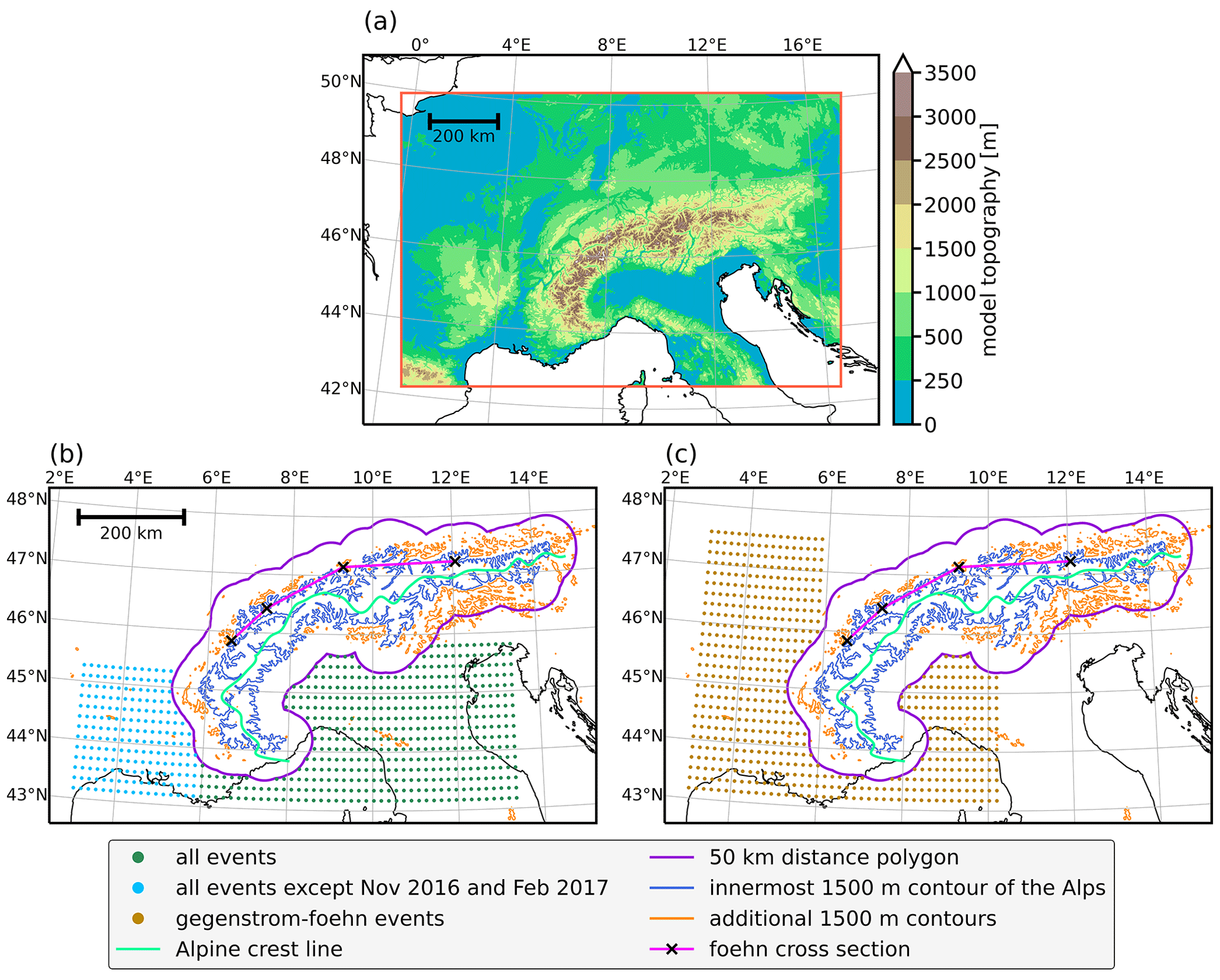
Figure 1(a) Model domain of the COSMO-1 hindcasts (red frame) and model topography (color map). (b) Trajectory starting points for all simulations except for the gegenstrom-foehn events. The green dots indicate the horizontal starting positions used for all of these events, while the blue dots denote additional starting positions not used for the November 2016 and February 2017 events (see text for further explanation). Additional geographic features comprise the 50 km distance polygon (violet contour), the innermost closed 1500 m contour of the Alps (blue), additional 1500 m contours (orange), the Alpine crest line (green), and the cross section used for the trajectory selection (the foehn cross section; pink line with black cross). (c) The same as (b) but for the two gegenstrom-foehn events (November 2019 (1) and February 2020).
The present study performed hindcast simulations using a model setup that closely follows the operational COSMO-1 setup used by the Swiss national weather service (MeteoSwiss). The computational domain of COSMO-1 encompasses the full Alpine range (1158 × 774 grid points; see domain in Fig. 1a). The simulations were conducted with a horizontal grid spacing of 1.1 km and 80 vertical levels, with the lowest half-level located 10 m above ground level (a.g.l.), and were integrated using a time step of 10 s. Over flat terrain and at some distance from the orography, there are 34 model levels below 2 , resulting in an average vertical grid spacing of ∼ 60 m. Subgrid-scale processes were parameterized except for subgrid-scale orographic drag and convection, which were assumed to be sufficiently resolved. Running the model without any convection parameterization is fortified by a sensitivity study of Vergara-Temprado et al. (2020), where they identified a similar performance of COSMO at 2.2 km horizontal grid spacing for both explicit convection and parameterized shallow convection. Therefore, and in alignment with the operational model setup of MeteoSwiss, all convection parameterizations were switched off for the simulations performed. The necessary initial and boundary conditions to drive the model were derived from operational COSMO-1 analyses provided by MeteoSwiss. As the analyses and the hindcasts are of the same resolution, this setup prevents the necessity of additional spin-up time at the beginning of the model integration.
An overview of the case studies (simulated period, observed foehn period, output frequency of three-dimensional fields, model version employed, predominant foehn type) is provided in Table A1. The events have been selected to represent the entire spectrum of different foehn types (Jansing et al., 2022). For most events, the model is initialized 6 h prior to foehn onset at Altdorf (a well-known Swiss foehn location; e.g., Richner et al., 2014), which is diagnosed using the enhanced version of the Dürr index (Dürr, 2008) aggregated to hourly resolution (Jansing et al., 2022). Furthermore, the simulations were run for 6 h after foehn cessation at Altdorf. For more details on the case study selection and the exact model setups, the reader is referred to Appendix A1.
As one of the first and only atmospheric models, COSMO has been ported to graphical processing units (GPUs) to leverage the performance advantages from modern hybrid computing architectures (Fuhrer et al., 2014; Leutwyler et al., 2016). Accordingly, most of the hindcasts have been conducted using the enhanced, GPU-capable version of COSMO (see Appendix A1).
2.2 Online trajectories
The COSMO model offers an option to calculate Lagrangian air parcel trajectories along with model integration (Miltenberger et al., 2013). These online trajectories are computed within the framework of the NWP simulation, thereby making use of the prognostic three-dimensional wind field at every native model time step (10 s). Both truncation and interpolation errors, two of the main error sources associated with the computation of trajectories, can be reduced when increasing the spatial and temporal resolution of the driving wind field. Online trajectories are thus of superior accuracy compared to the more traditional offline trajectories, which is particularly valuable when investigating non-stationary flows over complex terrain (Miltenberger et al., 2013). Since the numerical model integrates the governing equations forward in time, the online trajectory module is likewise limited to the calculation of forward trajectories. Therefore, it is imperative to release air parcels within all upwind regions that potentially contribute to the foehn flow within northern Alpine valleys. Consequently, trajectories have been started in extensive three-dimensional latitude–longitude boxes on the Alpine south side. The horizontal extent of these boxes varies between the different simulations (Fig. 1b, c and Table A2). Owing to the performance benefit of the GPU-enabled online trajectory module, which has been used for all simulations except November 2016 and February 2017, the number of trajectories per starting time has been increased for these simulations (compare the green dots to the blue dots in Fig. 1b). The different starting boxes for November 2019 (1) and February 2020 (Fig. 1c) compared to the other events (Fig. 1b) are motivated by the fact that these two events belong to the so-called gegenstrom-foehn type (see Table A1). During such events, a strong zonal large-scale flow causes a more westerly origin of foehn air parcels compared to other foehn types (Jansing et al., 2022). For more details on the exact setup of the online trajectory module, the reader is referred to Appendix A2.
Trajectories are selected if they, at first, intersect with the Alpine crest line (see green line in Fig. 1b and c) and, afterwards, intersect with a cross section in the lee of the Alps (the pink line in Fig. 1b and c; hereafter referred to as the foehn cross section) into a northerly direction and below 2500 m above mean sea level (a.m.s.l.). This selection procedure ensures that only trajectories traversing the Alpine ridge and, subsequently, diving into northerly foehn regions, are classified as foehn trajectories.
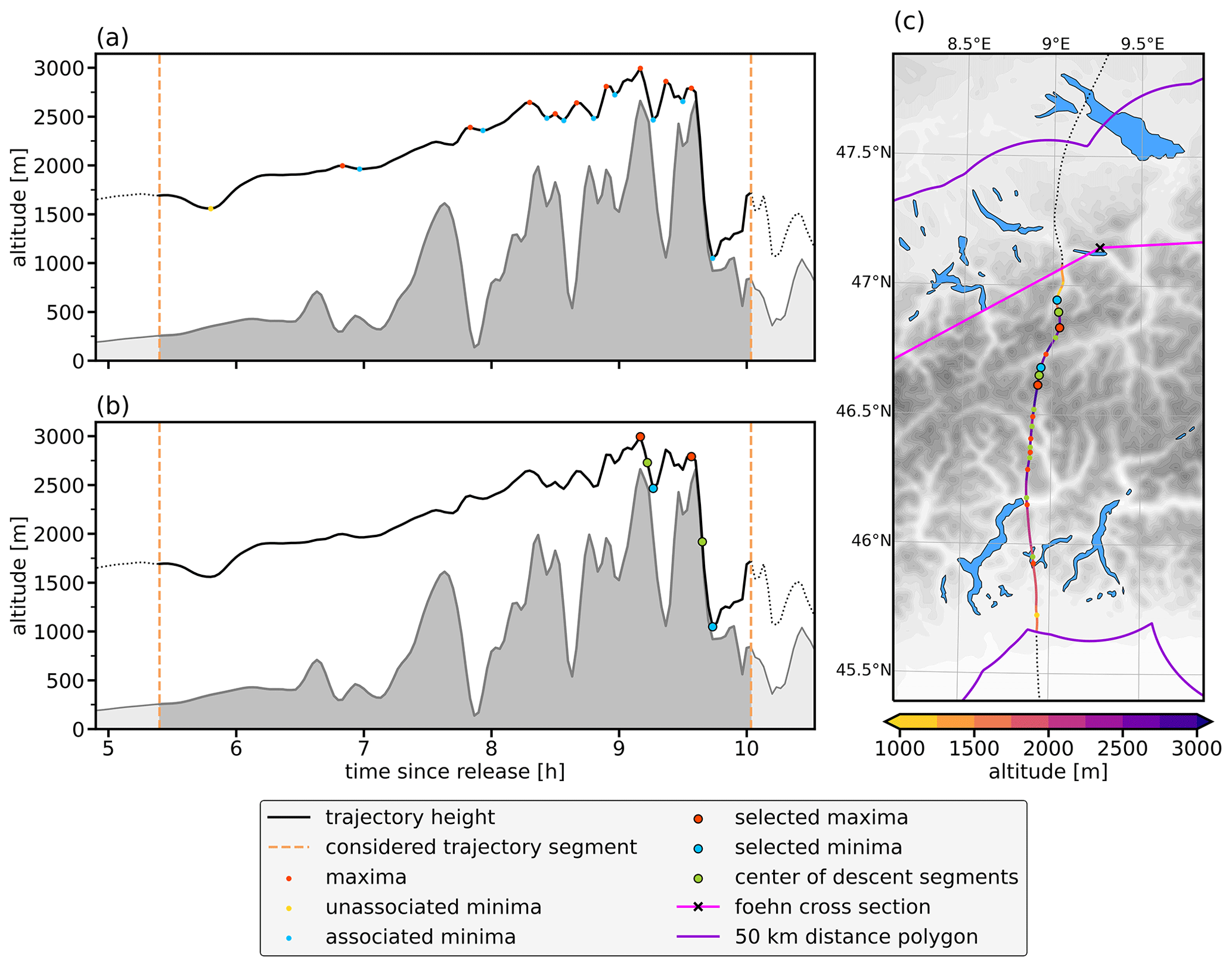
Figure 2Illustration of the algorithm used to identify segments of strong descent by means of an example trajectory from the March 2016 event. Panel (a) depicts the altitude a.m.s.l. of the trajectory. The considered trajectory segment is highlighted by the dashed orange lines. The red dots mark identified local maxima, blue dots the associated local minima, and yellow dots the unassociated minima. Panel (b) depicts the altitude a.m.s.l. of the trajectory and the selected descent segments fulfilling the magnitudinal and temporal criteria. Additionally, the center of each descent segment is indicated by a green dot. Panel (c) illustrates the horizontal pathway of the same trajectory, likewise indicating the local maxima, minima, and the selected descent segments.
2.3 Descent identification
In order to identify locations of strong descent, an algorithm is applied to each selected foehn trajectory (illustrated in Fig. 2):
-
Local maxima and local minima in the trajectory altitude are identified by comparing each trajectory altitude to its neighboring values, whereby the prominence needs to exceed 30 m. The prominence of a local maximum is defined as the height difference with respect to the lowermost closed contour line encompassing the respective maximum. The prominence of a local minimum, in turn, is defined as the height difference between the minimum and the lower of the two surrounding maxima that encircle the minimum. Applying a threshold in prominence ascertains that altitudinal fluctuations of a very small amplitude are excluded in the further processing.
-
Each minimum is assigned to a preceding maximum to obtain pairs of maxima and minima, corresponding to descent segments (red and blue points in Fig. 2a and c). If a trajectory first reaches a local minimum, this minimum is unassociated with any maximum and not considered for further analysis (yellow point in Fig. 2a and c).
-
Only segments with a descent of at least 500 m within a maximum time span of 30 min are kept. This filtering ensures that only rapidly occurring descent segments of substantial vertical magnitude are selected.1 The enlarged red and blue points in Fig. 2b and c highlight the two selected descent segments that fulfill these criteria in the present example.
-
The center point of each descent segment is identified by linear interpolation between the adjacent maximum and minimum (green points in Fig. 2b and c).
This procedure is applied to each trajectory, starting from the last trajectory time step prior to intersection with the Alpine polygon (violet contour in Fig. 2c) until the first time step after having intersected with the foehn cross section (pink line in Fig. 2c). Altogether, a total of 912 425 descent segments are identified in the 15 simulated cases. Note that multiple descent segments can be identified per trajectory.
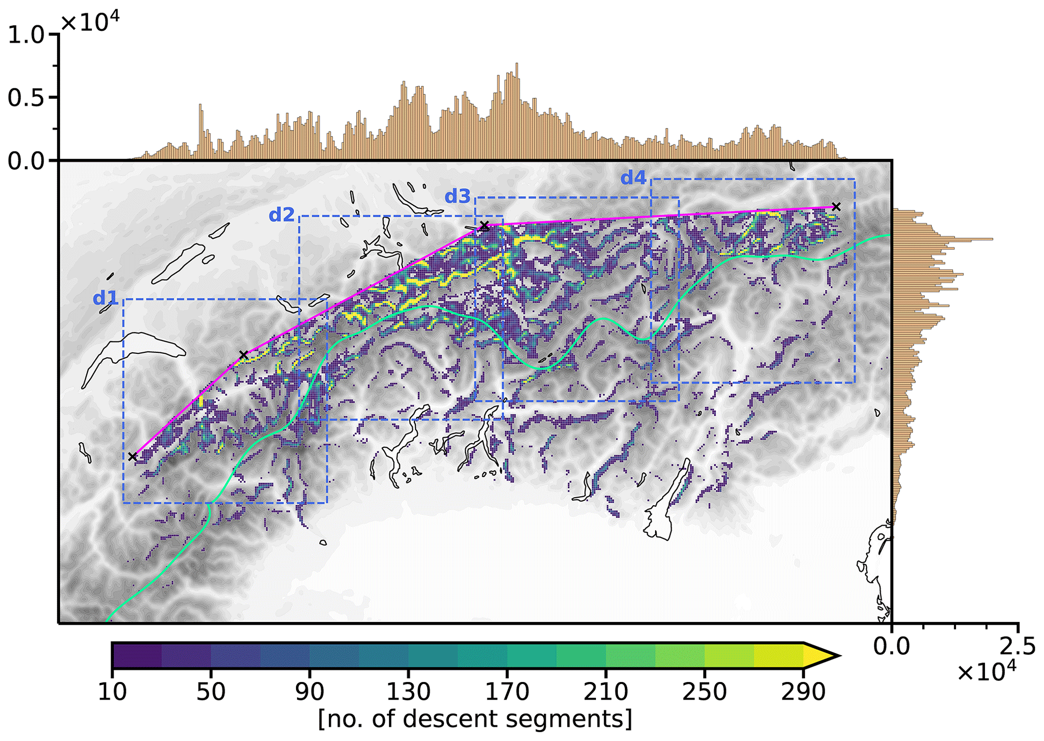
Figure 3Number of descent segments from all foehn events within equally spaced 0.01° × 0.01° bins on the rotated latitude–longitude grid (color map). Note that values below 10 are masked to enhance visibility. The pink line with black crosses indicates the foehn cross section, while the green line corresponds to the crest line (used for orientation). Additionally, the number of trajectories within each rotated latitude–longitude segment is shown by means of two histograms along the upper and the right edges of the map, respectively. The dashed blue boxes (labeled d1 to d4) denote four subdomains that provide a zoomed-in view of the descent regions in Fig. S2 in the Supplement.
3.1 Spatial extent of descent regions
Having identified strong descent along the air parcels (see Sect. 2.3), we first assess where along the Alpine arc the air parcels actually descend during south foehn. To this end, the center points of all descent segments (green dots in Figs. 2b and c) from the 15 foehn events are displayed in a two-dimensional, binned histogram (Fig. 3). In addition, one-dimensional histograms along the upper and right edges illustrate the variability in zonal and meridional directions, respectively. In all foehn regions, extending from the westernmost Haute-Savoie in France to the easternmost Ziller Valley in Austria, strongly descending air parcels are discernible. The number of descent segments however varies between the different regions. It peaks in an area covering the central Swiss Alps and the Rhine Valley, while fewer air parcels descend in the Western and the Eastern Alps (see also the histogram in the upper part of Fig. 3). Note that the area spanning the central Alps to the Rhine Valley also corresponds to the region where the overall highest number of foehn trajectories is selected. On a smaller scale, peaks in descent activity emerge in proximity to the incisions of major foehn valleys, such as for example the lower Valais, the Reuss Valley, the Rhine Valley, and the Wipp Valley (see the locations of the valleys in Jansing and Sprenger, 2022). This clearly highlights the relevance of major foehn valleys as preferential regions for strong descent of air parcels.
Although the identification method does not explicitly limit strong descent to regions north of the Alpine crest, descent indeed predominantly occurs within these areas (Fig. 3). This north–south gradient in descent activity is not surprising, as strong descent is expected to occur, if at all, downstream of an orographic obstacle (e.g., Durran, 1990). Instances of strong descent south of the Alpine crest are primarily confined to local mountain chains and valleys that exhibit an east–west orientation (e.g., the Valtellina in Italy). These mountain chains act as a local barrier to the southerly flow, allowing for leeside descent despite being situated on the southern side of the Alpine crest.
At the regional to local scale, a striking feature concerns the uneven spatial distribution of descent segments (Fig. 3). Instead, pronounced maxima in descent activity emerge, which we refer to as hotspots. These maxima are strongly confined in space and frequently situated in the immediate lee of elongated orographic obstacles, resulting in a correspondingly elongated shape of many hotspots. This observation highlights the significant influence of local topography, which serves as a natural anchor for the downslope flow during foehn events. A minority of the hotspots, however, also extend across the valley floor of foehn valleys (e.g., lower Valais, Reuss Valley, Rhine Valley). Furthermore, it is particularly highlighted that the overall strongest hotspot (see peaks in histograms along the edges of Fig. 3) emerges along the mountain chain of the Rätikon, whose slopes face towards the Rhine Valley in the west and towards the Walgau in the north (see Fig. 7 for orientation). Zängl et al. (2004a) also described the northern slopes of the Rätikon as a preferential region for descending motion, a finding clearly corroborated by our Lagrangian analysis of descent locations. Accordingly, this hotspot is subject to more detailed investigations in Sect. 4.
Moreover, most identified descent regions are not located in the immediate vicinity of the Alpine crest but rather in close proximity to the arrival locations of the respective air parcels (pink line in Fig. 3). However, there exist some noteworthy exceptions to this pattern, particularly in the upper Valais region. There, a considerable number of air parcels descends into the Valais and is presumably channeled downvalley. Such pathways of air parcels have also been observed during the November 2016 event (see Jansing and Sprenger, 2022). Additionally, several hotspots emerge in the tributaries of the upper Rhine Valley. It is worth noting that in this particular region, the main Alpine crest is situated at a greater distance from the arrival locations.
In the comprehensive analysis of descent locations, trajectories from all events were collectively considered to examine the spatial variability in descent activity. An extended investigation of the case-to-case variability, along with a sensitivity analysis involving different thresholds in altitude (Δz) and time (Δt), can be found in the Supplement (Sect. S1 and Figs. S3 and S4).
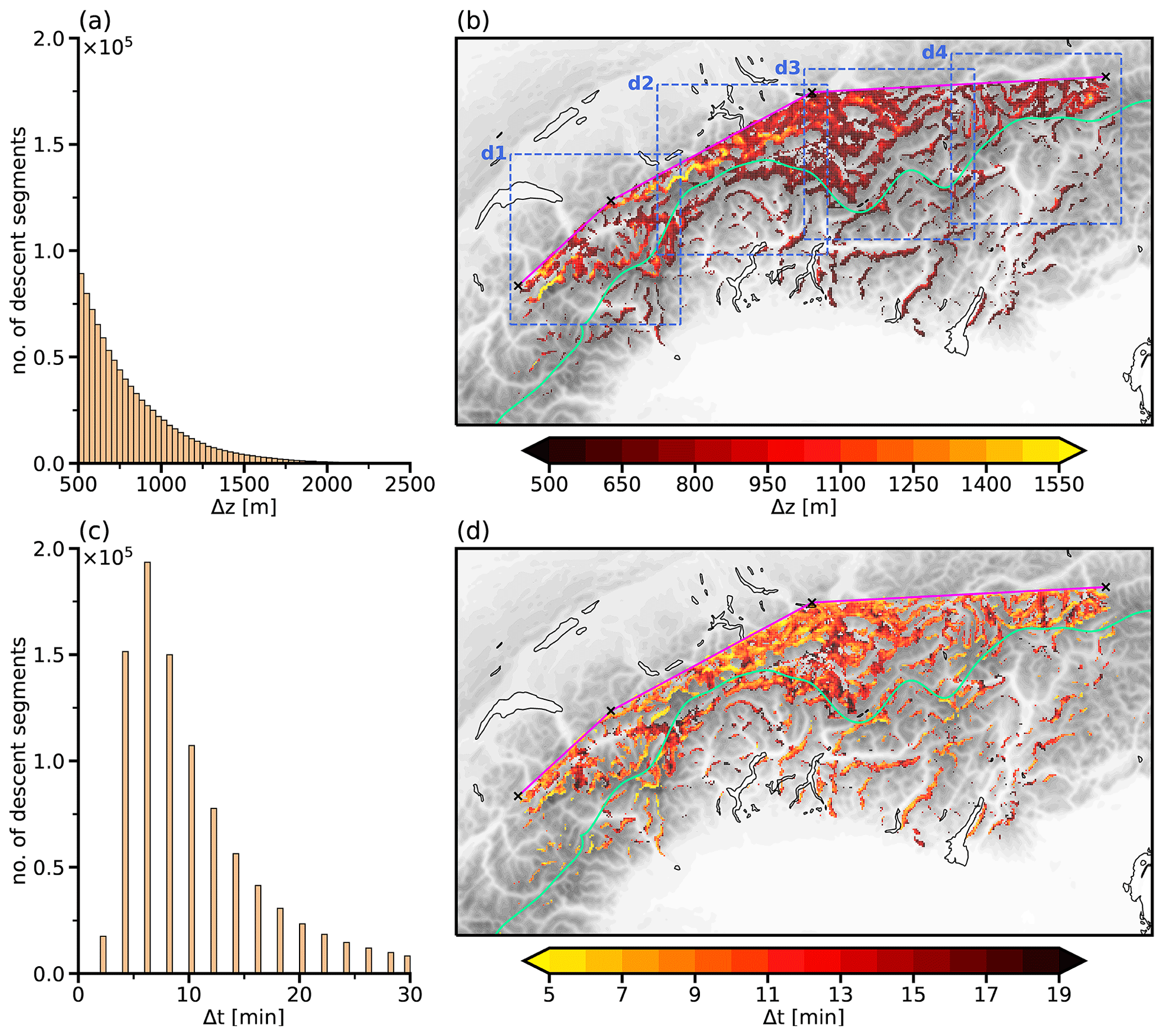
Figure 4Kinematic characteristics of foehn descent segments. Panels (a) and (c) display the histograms of the kinematic characteristics (Δz and Δt). Panels (b) and (d) show the same kinematic characteristics but in two-dimensional binned histograms (as in Fig. 3). The bins are colored according to the mean characteristics within each bin. The dashed blue boxes (labeled d1 to d4) in panel (b) denote four subdomains that provide a zoomed-in view of the descent characteristics in Figs. S5 to S8 in the Supplement.
3.2 Kinematic and thermodynamic characteristics of descent regions
The preceding section elucidated the distinct spatial variability of the descending motion related to foehn, establishing preferential regions of descent. But do these regions diverge in terms of the characteristics (e.g., magnitude, thermodynamic evolution) of the air parcels' descent, or do the air parcels descend uniformly across all foehn regions north of the Alps? To address these questions, the subsequent section explores the potential variability in the descent characteristics. In this regard, two different types of characteristics are of particular interest. The kinematic characteristics encompass the vertical magnitude of the descent segments (Δz) and their time span (Δt). The thermodynamic characteristics include the potential temperature difference (Δθ) and the specific humidity difference (Δqv) of the end points to the start points of each descent segment. To investigate all of these characteristics, one-dimensional histograms are used to illustrate their overall distribution and the range of typical values (Figs. 4a, c and 5a, c) and two-dimensional binned histograms to highlight the spatial variability (Figs. 4b, d and 5b, d).
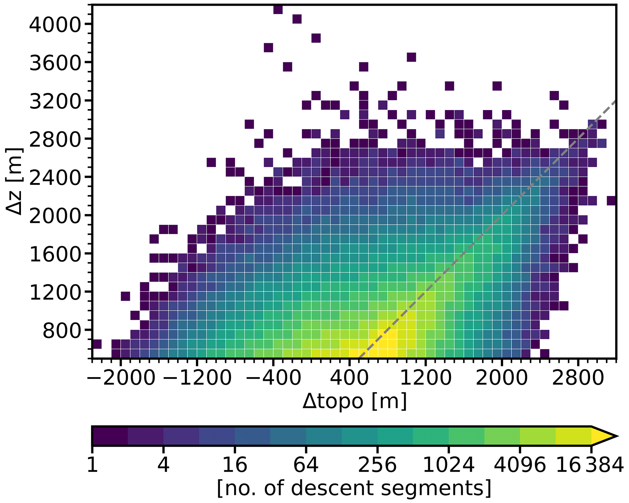
Figure 5Relation of the descent magnitude (Δz) to the change in the underlying terrain (Δtopo) in a two-dimensional histogram colored according to the number of descent segments within each bin. The 1:1 line is included as a dashed gray line. Note the exponential color scale.
Focusing on the kinematic characteristics, it becomes evident that the descent of air parcels exhibits substantial variations, in terms of both magnitude and time span. The frequency of descent segments decreases exponentially with increasing descent magnitude (Fig. 4a). Air parcels thus rarely descend more than 1500 m within one single descent segment. The time span to cover the descent ranges from 2 to 30 min; however most of the air parcels need about 4–10 min to descend (Fig. 4c).
The descent magnitude exhibits particularly strong spatial variability (Fig. 4b). Pronounced maxima emerge downwind of some of the highest peaks of the Western Alps, such as the Mont Blanc massif or the Bernese Alps, where mean values even exceed 1500 m. In stark contrast, the descent magnitude is substantially smaller in regions close to the Alpine crest (see green line in Fig. 4b). These spatial differences result from variations in the local terrain characteristics that appear to be strongly related to the descent: since valley incisions tend to be less deep in regions closer to the crest, the elevation differences between the local valleys and the surrounding mountain peaks are smaller, thus inhibiting descent of greater magnitude. In most of the localized hotspot regions, the mean descent magnitude is between 750 and 1000 m. Therefore, the terrain does not only determine the preferred locations for descent, but also to a large extent dictates its magnitude. This relation is further illustrated in Fig. 5. The descent magnitude (Δz) is closely correlated to the change in the underlying topography (Δtopo). Descent of a very large magnitude thus almost exclusively occurs along steeply sloping flanks on the leeside of the highest Alpine peaks.
The time span needed to cover the descent segments likewise varies regionally (Fig. 4c). However, no clear linkage to the local terrain characteristics emerges. While most regions exhibit a mean time span of approximately 7–11 min, some localized regions, especially in the Central Alps, are characterized by shorter descent time spans. The magnitude and the time span are not clearly anticorrelated, meaning that rapid descent (small Δt) does not need to be co-located with descent of a large magnitude (large Δz) and vice versa.
The clear correlation between the descent magnitude and the changes in the underlying topography strongly indicates that the downslope flow is often essentially terrain-following. One hypothesis is that mountain gravity waves, anchored to local peaks, are associated with the descent of foehn air parcels. Under this assumption, variations in the descent magnitude across different regions could be attributed to spatially varying wave amplitudes, which are, in turn, influenced by the local mountain height. However, considering the evident spread in Fig. 5, factors other than the local terrain certainly influence the descent magnitude as well. For instance, if descending air parcels reach their level of neutral buoyancy prior to arriving at the leeside valley floor, the descent magnitude will be less than the underlying change in elevation. Furthermore, other local factors potentially affect the descent characteristics, and these are discussed further in Sect. 4, focusing on the hotspot along the Rätikon.
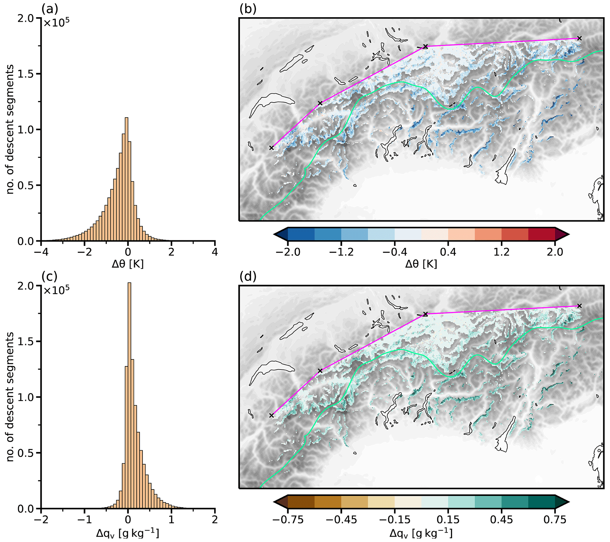
Figure 6The same as Fig. 4 but for the thermodynamic characteristics (potential temperature difference Δθ and specific humidity difference Δqv).
Subsequently to the kinematic characteristics, two thermodynamic characteristics are analyzed (Δθ, Δqv). The majority of descending air parcels experiences no noteworthy change in potential temperature (Fig. 6a). This finding implies that the descent happens approximately adiabatically, and the air parcels follow steeply downward-sloping isentropes in the lee of the mountain peaks. Nevertheless, the distribution of Δθ is slightly skewed towards negative values, revealing that a minor share of the air parcels experiences diabatic cooling. Similarly, most air parcels are not subject to specific humidity changes, yet a slight humidity uptake is registered for some of the descent segments (Fig. 6c). The minority of descent segments associated with diabatic cooling and a specific humidity increase is clearly co-located (Fig. 6b and d). They predominantly occur either south or a small distance from the Alpine crest. On the southern side of the Alps, the impinging air parcels during foehn oftentimes form clouds and precipitation. When these air parcels locally descend and therefore start to warm, the clouds and rainwater at least partially evaporate, resulting in diabatic cooling and a specific humidity gain. This peculiarity in the thermodynamic characteristics of descending air parcels south of the Alpine crest might also explain the relatively low number of descent segments in these regions (Fig. 3) and their small magnitude (Fig. 4b): the evaporative cooling during the leeside descent potentially reduces the amplitude of the local gravity waves and impedes stronger descent, an effect previously described by Zängl (2006). In contrast to the pattern south of the Alpine crest, a few regions north of the crest feature a minor increase in potential temperature. This diabatic heating is most probably caused by turbulent mixing within the stably stratified flow, as condensational heating cannot occur along descending air parcels, and radiative heating likely plays a minor role considering the short time spans of individual descent segments. Analogously, a local drying could be related to turbulent mixing of descending air parcels with drier air from higher levels.
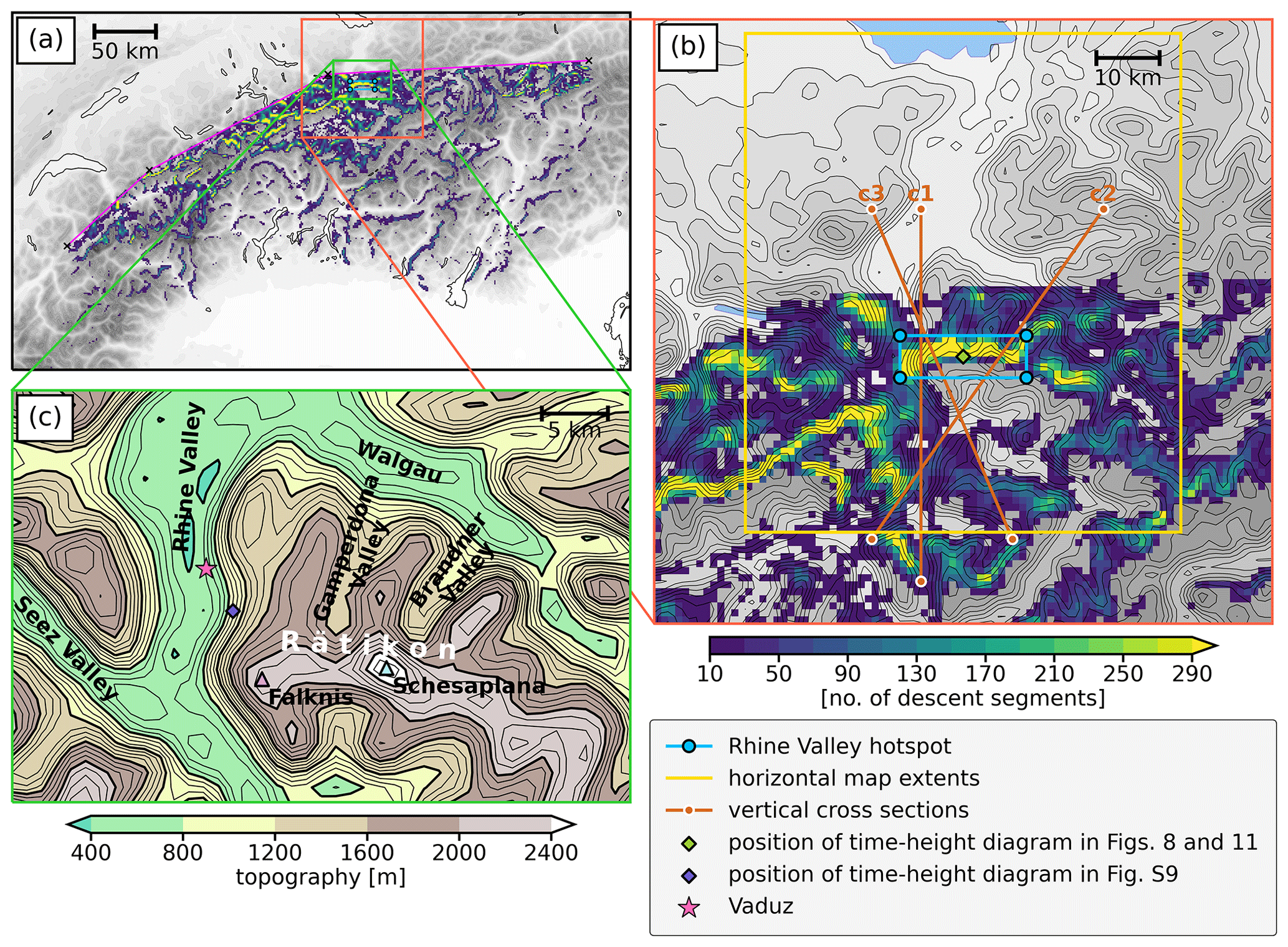
Figure 7Geographic overview of the region in proximity to the Rhine Valley hotspot. Panel (a) depicts the extended Alpine region that has been focused on in Sect. 3. Panel (b) shows an enlarged map of the central and lower Rhine Valley, with the blue box indicating the investigated hotspot. The yellow subregion marks the extent of the maps depicted in Figs. 9 and 12. The brown lines show the locations of the vertical cross sections (labeled c1 to c3), which are displayed in the two case studies (Figs. 9 and 12). The green marker depicts the location of the time–height diagrams in Figs. 8 and 11. Panels (a) and (b) are both colored according to the number of descent segments within equally spaced bins (the same as in Fig. 3) and include the topography of COSMO-1 in gray shading (and contours with 200 m spacing in b). Panel (c) shows an enlarged contour map of the Rätikon mountain chain using the model topography (color map and contours with 100 m spacing). Important valleys, mountain peaks, and locations are labeled. The dark-blue marker shows the location of the time–height diagram in Fig. S9 in the Supplement.
So far, the spatial variability in the descending motion of foehn air parcels and the associated characteristics have been investigated on Alpine to regional scales. Strong descent turned out to be spatially confined to distinct hotspots in the lee of local mountain chains and peaks. On this basis, the next goal of this paper is therefore to examine one of these hotspots. This is tackled by focusing on the hotspot along the Rätikon (hereafter denoted as the Rhine Valley hotspot). The selection of this hotspot is motivated by two reasons: first of all, it coincides with the location where the overall number of descent segments reaches its maximum (Fig. 3). Secondly, the northern slopes of the Rätikon close to Vaduz (pink star in Fig. 7c) have previously been identified as a preferential region for descending motion during MAP (Zängl et al., 2004a), which allows us to discuss our results in relation to existing literature. The following in-depth analysis of the Rhine Valley hotspot unravels the ambient atmospheric conditions related to strong descent and reveals the drivers of temporally varying descent activity by means of two case studies (Sect. 4.1 and 4.2). To this end, the Rhine Valley hotspot is defined as a rectangular box (blue box in Fig. 7b), and all descent segments whose center points lie within this box are selected for the analysis. For the two case studies, horizontal maps (yellow frame in Fig. 7b) and vertical cross sections (brown lines in Fig. 7b) are additionally utilized to investigate the meteorological conditions in the immediate vicinity of the hotspot.
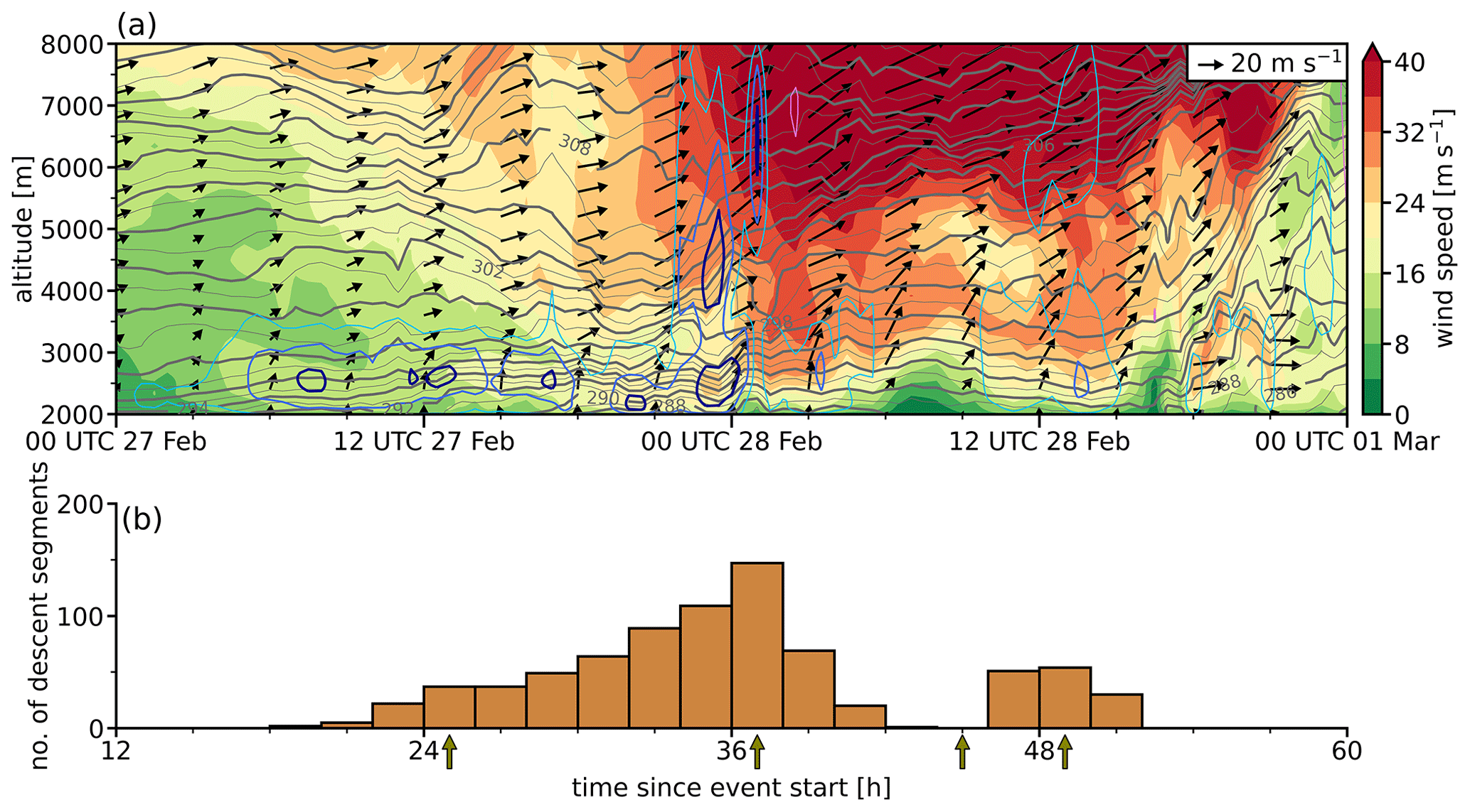
Figure 8(a) COSMO-based time–height diagram of horizontal wind speed (color map and arrows) in the center of the hotspot region for the February 2017 event (the location of the time–height diagram is indicated by the green marker in Fig. 7b). The arrows pointing to the right correspond to eastward winds and arrows pointing upward to northward winds. Isentropes are indicated as gray contours with a spacing of 1 K. Additionally, vertical winds are displayed using blue and violet contours for negative and positive values, respectively (spacing of 1 m s−1; starting from ± 1.5 m s−1). (b) Temporal evolution of the number of descent segments in the Rhine Valley hotspot within 2-hourly windows. The selected time instants for the horizontal and vertical cross sections shown in Figs. 9 and 10 are highlighted by olive-colored arrows along the x axis.
4.1 February 2017 case study
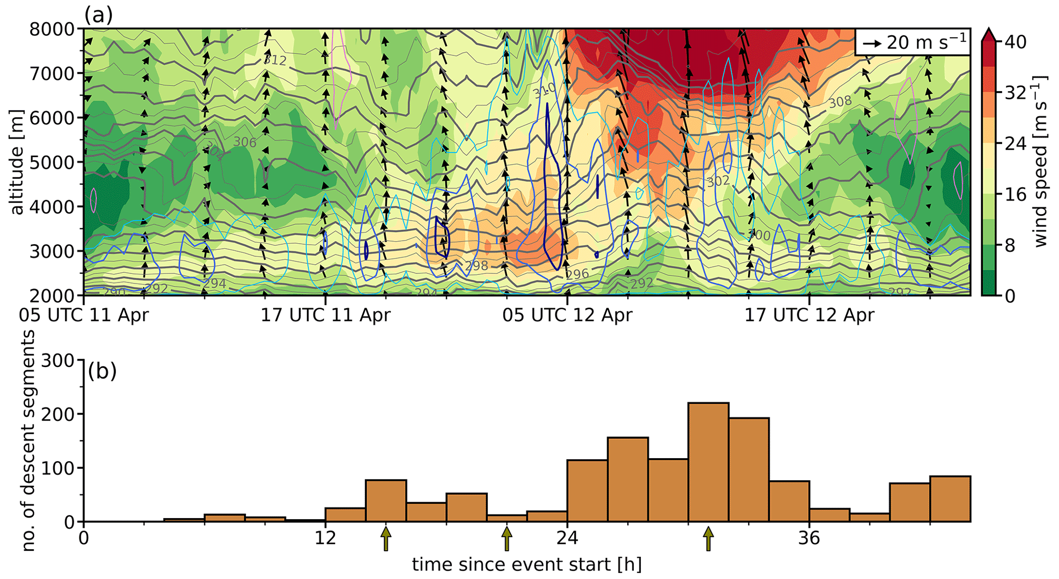
In the early afternoon hours of 27 February 2017, the observational-based foehn index (Dürr, 2008) showed that foehn broke through in Vaduz (see also Jansing, 2023), which corresponds to 25 h since the event start.2 In accordance with the observed onset of foehn at the surface, the first descending air parcels are detected a few hours prior to foehn onset at Vaduz (Fig. 8b). Thereafter, the number of descent segments increases over time and peaks after 37 h, followed by a sharp decrease and a transient break in descent activity, before a second period with a lower number of descent segments is detected between 46 and 52 h since the event start. The goal of the following section is to explain this very distinct temporal evolution of the descent activity by linking it to the local atmospheric conditions during the course of the event.
The February 2017 event is categorized as a deep-foehn event and occurred downstream of a broad upper-level trough and a cold front that approached the Alpine region from the northwest (not shown). At first, weak to moderate west-southwesterlies prevail at all levels in the region of the hotspot (Fig. 8a). After 20 h, the winds below 3 km start to blow from the south sector. Hence, the horizontal winds turn clockwise with height, and a pronounced warming in the mid-troposphere sets in. At lower altitudes, strong downward motion is discernible (blue contours in Fig. 8a). Concurrently, the west-southwesterlies at mid- and upper-tropospheric levels continuously intensify until 35 h since the event start. In the lower troposphere, between 2–3 km, a layer of high stability forms during this time period. In the time window of 30–37 h, a low-level wind maximum occurs within the region of the stable layer, which aligns well with the peak period of descent activity (Fig. 8b). As the low-level winds reach their highest intensity, the downward motion extends throughout the troposphere. Subsequently (at 40 h), the wind speeds below 3 km temporarily decrease, before a second maximum is detected at 50 h. This temporal evolution likewise aligns with the transient break and secondary peak in descent activity. Finally, the winds below 4 km turn to the northwest, and isentropes rise to higher altitudes, indicating the arrival of the cold front. Overall, a very clear correspondence of the large-scale winds above crest levels and the descent activity is identified (cf. Fig. 8a and b).
To further examine how the local conditions are related to the temporal evolution of the descent activity during the February 2017 event, four interesting time instants (see olive-colored arrows in Fig. 8b) are selected and further investigated using horizontal maps and vertical cross sections (25 h: onset of descent but still weak descent activity, 37 h: peak descent activity, 45 h: a temporary break, 49 h: secondary peak before final cessation). It is highlighted where and under which ambient conditions air parcels descend in the hotspot region.
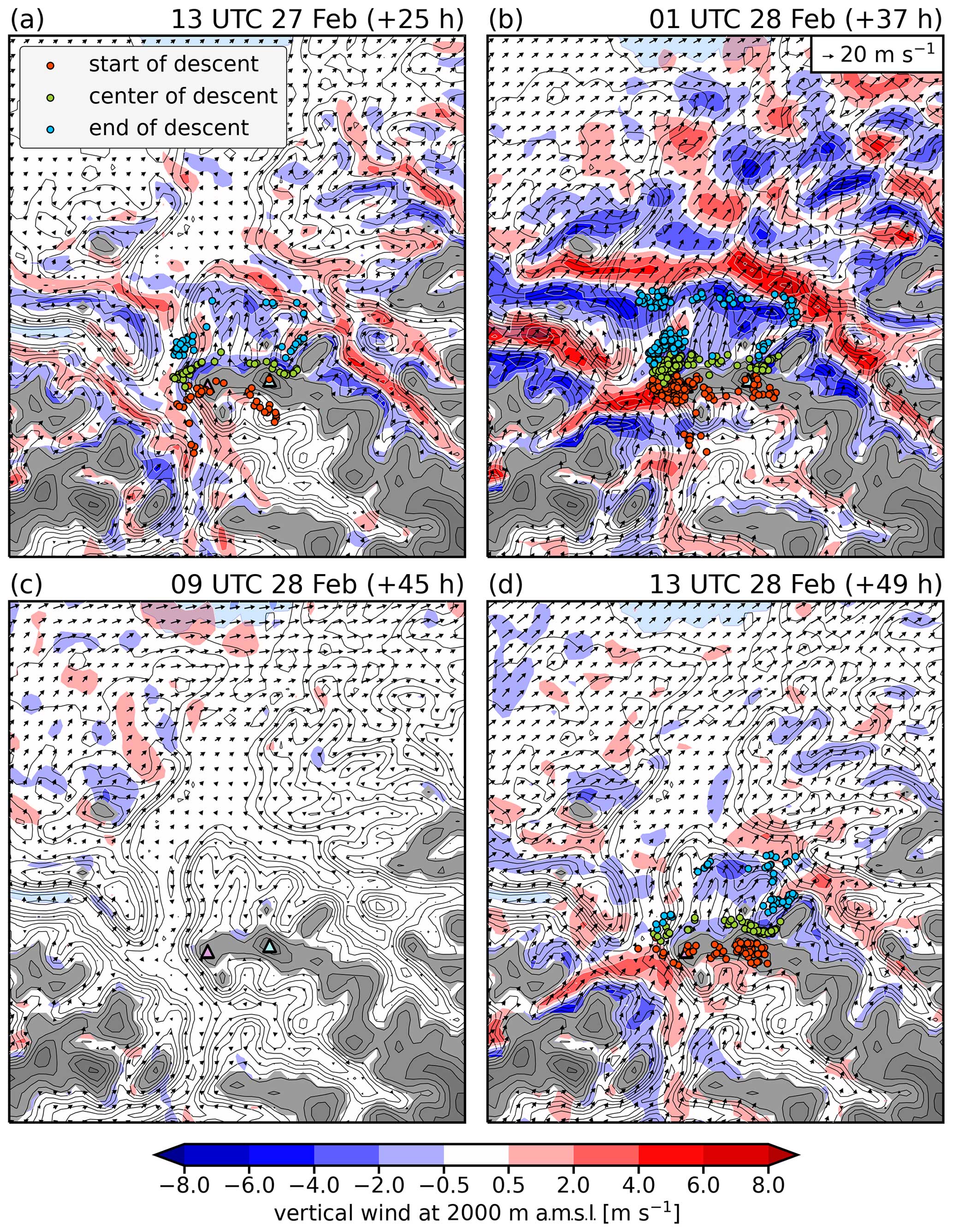
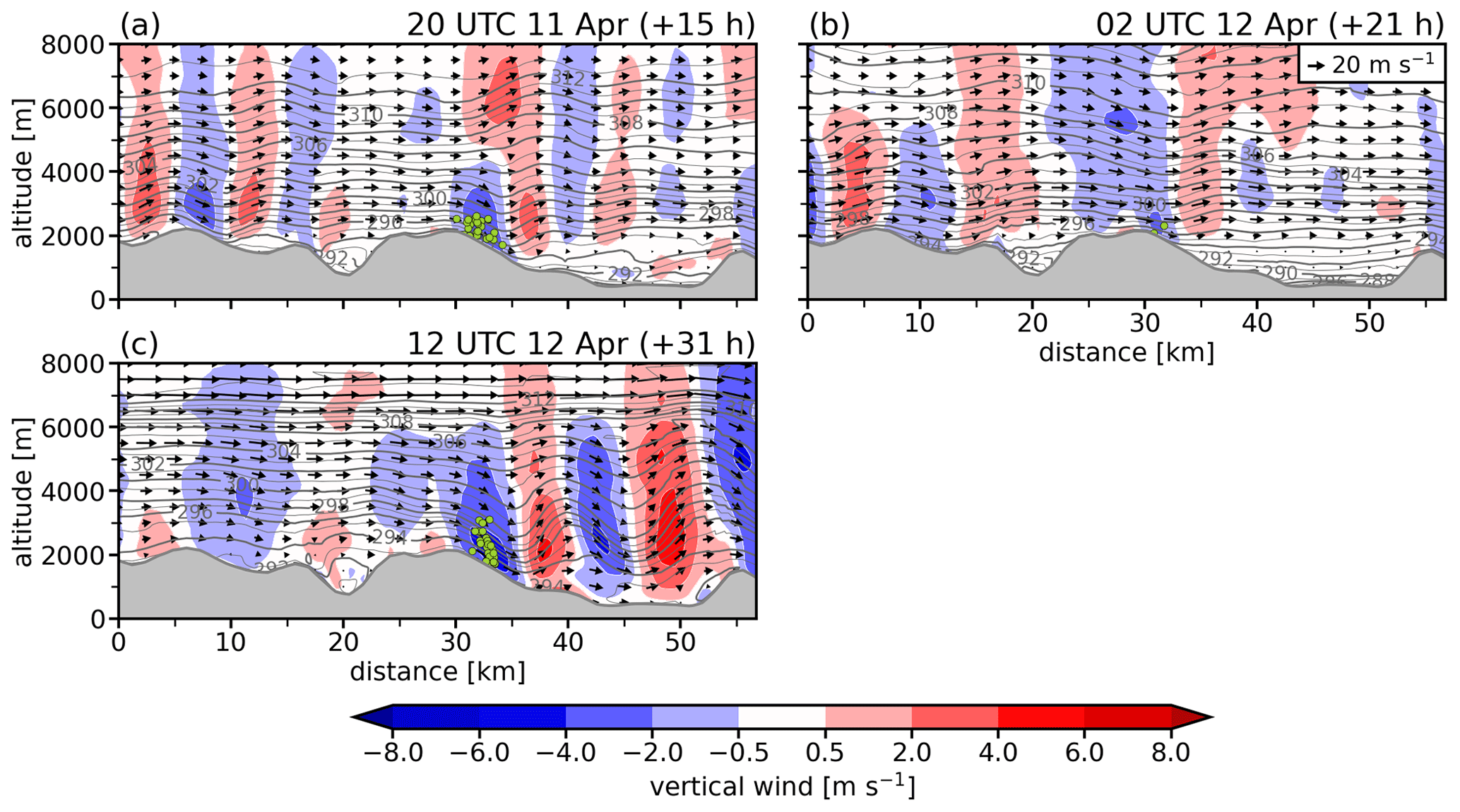
Figure 9Vertical wind (color map) and horizontal wind (arrows) at 2000 for (a) 13:00 UTC on 27 February 2017, (b) 01:00 UTC on 28 February 2017, (c) 09:00 UTC on 28 February 2017, and (d) 13:00 UTC on 28 February 2017. Additionally, the figure shows the start (red), center (green), and end positions (blue) of the trajectory descent segments that occurred within a 2-hourly window centered around the displayed dates. The COSMO topography is included in the background for orientation (gray shading starting at 2000 and contours with 200 m spacing). The peaks of the Falknis and the Schesaplana (see also Fig. 7c) are indicated as pink and light-blue triangles, respectively.
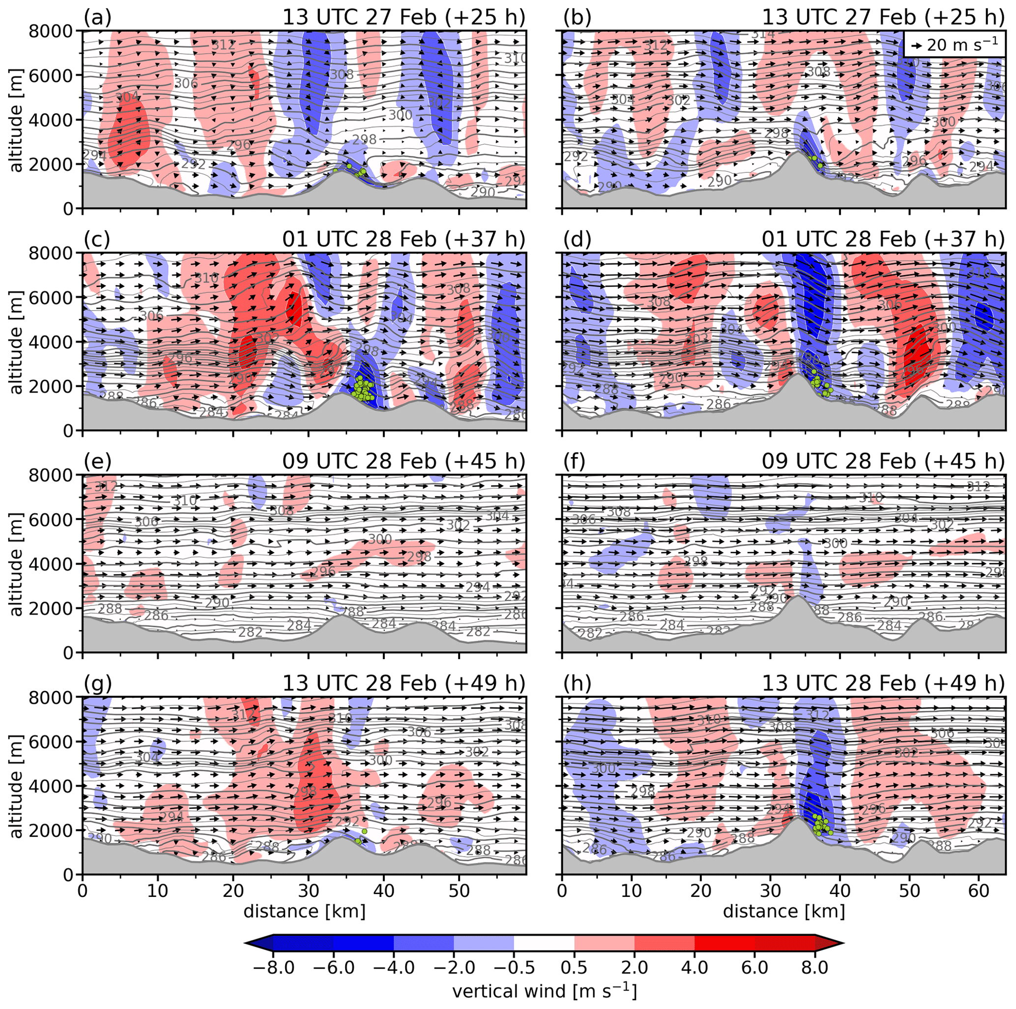
Figure 10Vertical cross sections of vertical wind (color map), isentropes (gray contours), and wind along cross sections (vectors). The topography is indicated by gray shading. The left column shows the cross section c1 (a, c, e, g), while the right column shows the cross section c2 (b, d, f, h). The four rows correspond to the four selected time instants (see also titles of each panel). Descent segments, which are located closer than 2 km to the cross section, are indicated as green dots.
The first time instant, 25 h after the event start, corresponds to the time the foehn reached Vaduz. While weak southwesterly winds prevail above crest height (Fig. 8a), elevated wind speeds at 2000 (Fig. 9a) are restricted to the northern slopes of the Rätikon and the upper Rhine Valley at this time. Two distinct groups of descending air parcels in the west and east of the hotspot area are discernible (Fig. 9a). The western air parcels start to descend along the northwest slope of the Falknis peak (pink triangle in Fig. 9a). They reach levels of 1 (not shown) when arriving over the Rhine Valley floor close to Vaduz. The eastern air parcels originate to the southwest of the Schesaplana and subside into the Brandner Valley (see Fig. 7c). Both groups of air parcels descend within regions of moderate downward motion (2–4 m s−1). The two vertical cross sections during the same time instant (Fig. 10a and b; see lines c1 and c2 in Fig. 7b), which traverse both descent regions in the lee of the Falknis and Schesaplana, unveil the presence of two gravity waves at low levels. These gravity waves emanate downwind of the two local peaks. They do not propagate vertically; instead both feature a convectively unstable region where the isentropes attain vertical orientation. Due to relatively weak impinging flow, the flow upstream of both peaks is, to a large extent, blocked, and a nonlinear wave regime establishes. Such a regime is typically reminiscent of nonlinear phenomena such as wave breaking (e.g., Durran, 1990). In addition, the analysis reveals distinct features reminiscent of hydraulic flow along both vertical cross sections. These features include an asymmetric flow pattern characterized by accelerated airflow downstream of the peaks; a rebound in a hydraulic jump as the flow adjusts to a new equilibrium level downstream; and the presence of a less stably stratified layer with weak winds on the downstream side, separating the descending foehn flow from the flow aloft. Overall, these observations indicate that the across-barrier density differences play an important role in the descent at this time.
A total of 12 h later (37 h since the event start), the peak in the descent activity has been reached (Fig. 8b). During this time instant, substantially stronger horizontal winds are observed at 2000 (Fig. 9b). Accordingly, intense wave activity of a larger amplitude is registered in the region of the Rhine Valley, as can be seen by alternating regions of strong upward and downward motion. The majority of trajectories descends along the northwestern slope of the Falknis (Fig. 9b) within downward motion in the immediate lee that is associated with a gravity wave. Considering the two vertical cross sections at the same point in time (Fig. 10c and d), a striking feature constitutes the abovementioned stable layer between 2.5 and 4 Pronounced vertical variations in static stability are known to inhibit vertical wave propagation (e.g., Jackson et al., 2013; Durran, 2015). Indeed, the gravity wave downwind of the Falknis seems to be partially trapped within the stable layer below 4 km. Downstream of the main peak, further mountain waves are discernible. However, it remains unclear whether this wave activity actually originates from the Falknis or is primarily caused by secondary peaks to the north, which potentially excite additional gravity waves. Since the mountain wave in the lee of the Schesaplana is able to propagate vertically (Fig. 10d), the ambient conditions do not seem to clearly favor the formation of horizontally propagating lee waves.
In the region to the northwest of the Falknis, which is associated with the strongest descent activity at this time instant (37 h since the event start), the orography features a local concavity. The concave shape of the terrain redirects the low-level flow, and, consequently, southeasterlies prevail close to the surface despite the southwesterlies at higher levels (see time–height diagram in Fig. S9a). This peculiarity of the local terrain presumably deflects the descending air parcels along the northwestern slopes of the Falknis and therefore promotes the descent into the valley atmosphere of the Rhine Valley.
The next highlighted time instant (45 h) corresponds to the time when a temporary break in descent activity is registered. While the southwesterlies continue to blow in the middle and upper troposphere, the wind speeds dramatically decrease below 3 km (Fig. 8a), and the stratification increases (Fig. 10e and f). Below 2 km, the conditions within the Rhine Valley and along the slopes of the Rätikon are essentially calm. As a consequence of the weak winds at crest level and the increased stability at low levels, no notable wave activity and no vertical motion is present (Figs. 9c and 10e, f), which explains the temporary break in descent activity. Based on horizontal maps of the low-level wind field of the region, a transient interruption of the foehn occurred (not shown).
In the early afternoon of 28 February (49 h since the start of the event), a second, weaker peak in descent activity was detected (Fig. 8b). Compared to 4 h earlier, the southwesterly winds at 2 slightly reintensified, and the low-level stability decreased (Fig. 9d). As a result, a vertically propagating gravity wave forms downwind of the Schesaplana (Fig. 10h), and air parcels are transported into the Brandner Valley. Interestingly, the descent activity is now primarily concentrated in this region. In the lee of Falknis, only a weak downslope flow is discernible (Fig. 10g). Minor changes in the local ambient conditions, such as local wind speed and direction or the absence of a stable layer, appear to inhibit the formation of a mountain wave or a hydraulic jump structure as observed in earlier times (Fig. 10a and c). However, further scrutiny would be required to elucidate the conditions provoking the formation of gravity waves in the lee of the Falknis.
The investigation of these four time instants shows a clear correlation between the number of diagnosed descent segments and the presence and intensity of mountain gravity waves in this region. This finding clearly demonstrates the intrinsically coupled nature of these two phenomena. The observed amplitude of the waves is influenced by the wind speed and direction of the impinging flow. Furthermore, the local topographic concavity to the northwest of the Falknis seems to favorably steer descending air parcels downward into the boundary layer of the Rhine Valley.
4.2 April 2018 case study
In the following, a second case study of the April 2018 event is presented with the goal to further illustrate the diversity of descent characteristics and to identify differences with respect to the main findings of the previous section.
The synoptic situation during the April 2018 event was characterized by a cutoff low over Spain and southern France, instead of an upper-level trough as in the February 2017 case (not shown). The cutoff induced a synoptic environment conducive to the formation of south foehn (see also Jansing, 2023). Related to the synoptic weather evolution, winds in the middle to upper troposphere above the hotspot region were relatively weak during most of the event, except for a period from 25 to 35 h, when strong southerly winds were detected at upper levels (Fig. 11a) due to the approach of the cutoff. Except for this period, the strongest winds were actually confined to a layer below 4 km. There, the horizontal winds blew from the south to southeast and reached their maximum 20–25 h after the start of the event at an altitude of 3 km. The lower troposphere was not only associated with stronger winds, but the stratification was also more stable compared to the middle and upper troposphere. Several periods of stronger downward motion alternated with intermittent periods of weak vertical motion.
The temporal evolution of descent activity during the April 2018 event differs from that of the February 2017 event (cf. Figs. 8b and 11b). During the event, several periods of enhanced descent activity interchange with periods of low activity. In general, the strongest descent is diagnosed in the time span of 25–35 h since the event start. In contrast to the February 2017 event, the April 2018 event does not show a clear co-variability of descent activity and impinging wind speeds. Thus, other local factors seem to play a crucial role in this case. To investigate this in more detail, three time instants (see olive-colored arrows in Fig. 11b) with different descent activities are selected to investigate the influence of local atmospheric conditions (15 h: the first, albeit weak, maximum of descent activity; 21 h: weak descent activity despite strong wind speeds above the crest; 31 h: peak of descent activity).
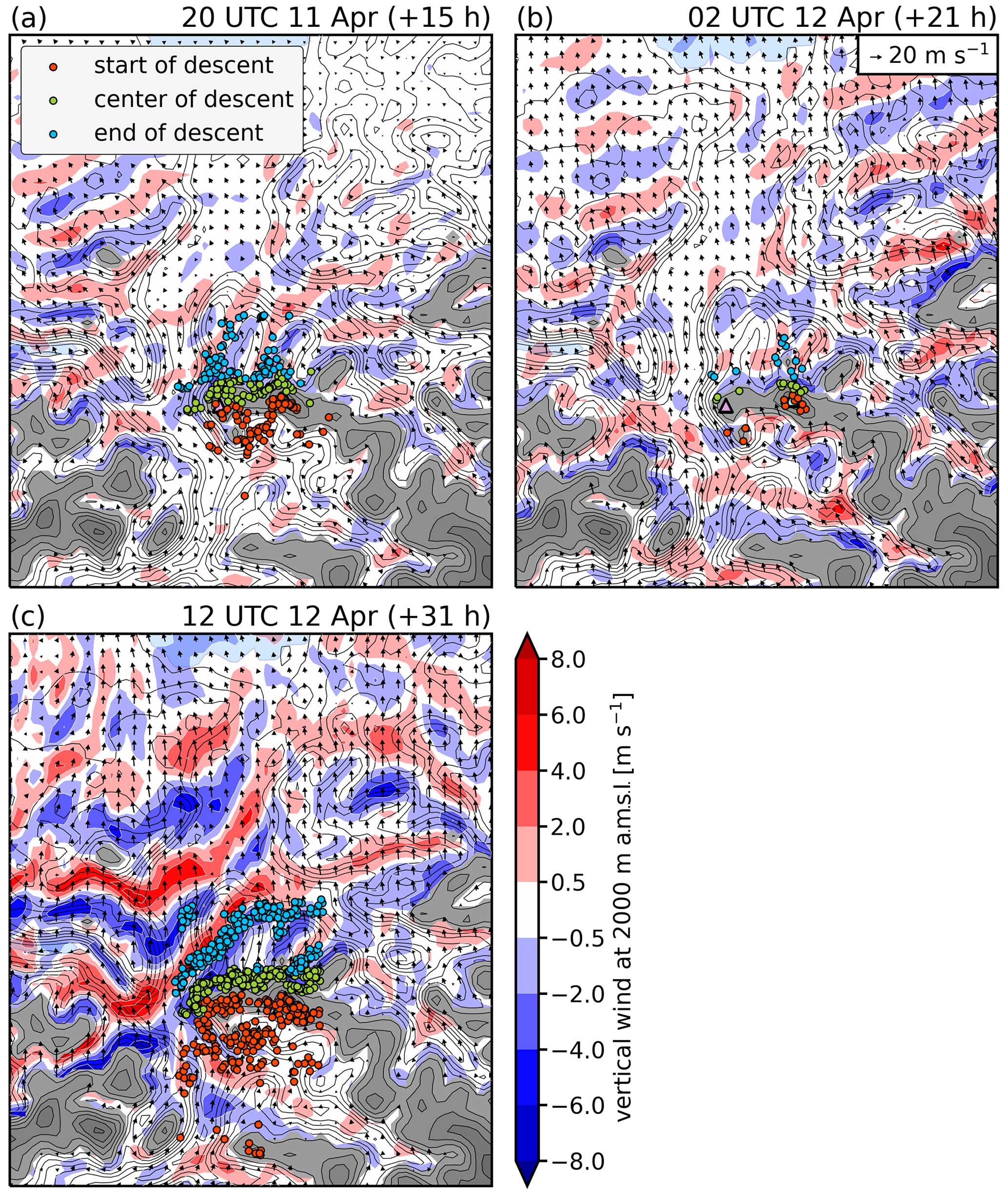
Figure 12The same as Fig. 9 but for the April 2018 event and (a) 20:00 UTC on 11 April 2018, (b) 02:00 UTC on 12 April 2018, and (c) 12:00 UTC on 12 April 2018.
The first highlighted time of the event (15 h) also corresponds to a first maximum in descent activity. Above the peaks of the Rätikon, moderate southeasterly winds prevail (Fig. 11a). The Falknis and the Schesaplana again excite two gravity waves, which are associated with the descending motion downwind of both peaks (Fig. 12a). On the one hand, air parcels descend along the northwestern slope of the Falknis into the wave trough of a horizontally propagating lee wave (Fig. 13a). On the other hand, air parcels also descend within a gravity wave to the northeast of the Schesaplana into the Gamperdona Valley (see Fig. 7c for orientation). Due to its position relative to the Schesaplana summit, the latter valley seems to be reached more easily by foehn air parcels when southeasterly rather than southwesterly winds prevail.
A total of 6 h later, 21 h after the start of the event, the registered descent activity was low (Fig. 11b). However, this seems counterintuitive given the ambient conditions at that time. In fact, the horizontal winds in the lower troposphere even reached their maximum during this period (Fig. 11a). Focusing on the hotspot region itself, the downslope winds in the lee of the Falknis are less pronounced at 2 km and essentially absent at lower altitudes (not shown). The vertical cross section c3 (Fig. 7b) shows that although a weak mountain wave is present adjacent to the Falknis peak, the downward vertical velocities do not extend below 1.8 km (Fig. 13b). This may be due to the stable stratification in the Rhine Valley during nighttime (see contracted isentropes), which prevents a further penetration of the wave signal into the valley atmosphere. Due to the stable valley atmosphere formed by nocturnal cooling, descending air parcels quickly reach their level of neutral buoyancy, and further descent is hindered. The cold-air pool thus produces a smooth virtual topography that limits the descent, as also described in Armi and Mayr (2015). Moreover, it is known that cold-air pools formed by nocturnal cooling effectively absorb the wave energy of trapped lee waves and thus strongly dampen their amplitude (Jiang et al., 2006).
Finally, the time associated with the strongest descent activity is examined (31 h). The impinging flow above the peak level now comes from the south sector. The amplitude of the horizontally propagating waves is substantially larger than before, especially over the valley axis of the Rhine Valley (Fig. 12c). Downward motion is observed in the lee of the entire Rätikon. Thus, the descending air parcels are linearly aligned along the northern slopes of the mountain chain. Similarly to what occurred during February 2017, air parcels descend along the northwestern slope of the Falknis into the Rhine Valley and into all northern tributaries of the Rätikon. The vertical cross section reveals the presence of a horizontally propagating lee wave of a larger amplitude than before (Fig. 13c). Note that the descending air parcels adjacent to the slope are potentially able to reach the neutrally stratified valley atmosphere below 1.7 km. These air parcels can thus in principle all be transported to the surface by vertical turbulent mixing within the boundary layer. This mechanism could also explain the cluster of air parcels arriving near Vaduz (Fig. 12c).
The April 2018 event is, in contrast to February 2017, characterized by intermittent descent activity that cannot merely be explained by variations in the impinging flow. Rather, the investigation indicates a pronounced influence of the daily cycle. While the stable stratification at night inhibits air parcels to subside into the valley atmosphere, a well-mixed boundary layer during the day promotes the penetration of foehn air parcels towards the valley floor. The important role of diurnal heating in increasing the potential temperature of the valley air and thereby facilitating the descent of foehn air parcels has been documented previously (Mayr and Armi, 2010). It is considered the primary explanation for the pronounced daily cycle of the climatological foehn frequency at many Alpine stations (Mayr et al., 2007; Gutermann et al., 2012).
5.1 Comparison to the MAP literature
There exist both analogies and discrepancies between our study and the existing MAP literature, which are briefly discussed in the following. For instance, Zängl et al. (2004a) diagnosed descending motion during a foehn event in the Rhine Valley by considering surface potential temperature maps. Similarly, variations in surface potential temperature in the Wipp and Ziller valleys were attributed to the different source altitudes of air (Zängl et al., 2004b) subsiding into these valleys. Gohm et al. (2004) identified several mountain ridges with leeside-descending motion using surface potential temperature and the vertical wind field. Among these regions was the ridge encompassing the Patscherkofel, which aligns with one of the hotspots identified in our Lagrangian descent analysis (see Fig. S2d). Focusing on the Rhine Valley, Zängl et al. (2004a) identified a distinct maximum in surface potential temperature north of Vaduz and attributed it to the descent along the Rätikon. This finding agrees well with our results, where the northern slopes of the Rätikon emerge as a major hotspot for descent.
The MAP publications focusing on IOP 10 revealed that downward-sloping isentropes, and hence descending motion, occur within vertically propagating gravity waves (Zängl et al., 2004a). In the region of the Wipp Valley, an overturning of the isentropes, commonly associated with wave breaking, has been diagnosed (Gohm et al., 2004; Zängl et al., 2004b). However, our second case study (April 2018) suggests the presence of propagating lee waves at the time of the strongest descent activity. Still, such a pattern of trapped lee waves has previously been reported to occur during south foehn (Zängl and Hornsteiner, 2007). Overall, it remains unclear whether there exists a wave regime that is particularly common during periods of strong descent. Another aspect beyond the scope of this study pertains to the role of below-cloud evaporation of precipitation in stabilizing the atmosphere and thus dampening the amplitude of gravity waves, as described by Zängl (2006). Nonetheless, vertical cross sections of the hydrometeors during the April 2018 event indicate no strong influence of evaporating hydrometeors on the stability of the valley atmosphere, at least at the times studied (not shown). In the local descent hotspots south of the Alpine crest, the abovementioned effect is likely not negligible, since these air parcels experience evaporative cooling during their descent.
An interesting side note concerns the preferential descent of foehn air parcels into the Brandner Valley when large-scale southwesterly to southerly flow prevails. In fact, Steinacker et al. (2003) have already diagnosed a gravity wave along the leeside slopes of the Rätikon based on a model simulation. They attributed the frequent restriction of the foehn to the upper part of the Brandner Valley to the wave-induced perturbation in the surface pressure. However, an investigation of this local interaction between the downvalley propagation of the foehn and the gravity field aloft was beyond the scope of this paper and would require a higher-resolution simulation.
5.2 What other factors influence the descent?
The presented analysis proposes a strong influence of the diurnal cycle on the descent of foehn air during the April 2018 case study. Potentially, the nocturnal minimum in descent activity is caused by the stable stratification of the valley atmosphere, forming a smooth virtual topography below which the flow cannot descend. This finding is consistent with prior research claiming that the descending flow must at least have the same potential temperature as the existing leeside valley air mass for the flow to descend (Mayr and Armi, 2008; Armi and Mayr, 2011, 2015). Furthermore, nocturnal cold-air pools are known to strongly attenuate the amplitude of gravity waves (Jiang et al., 2006). In alignment with this, previous studies have stressed the importance of daytime heating for foehn breakthrough (Mayr and Armi, 2010), and the climatological foehn frequency at most surface stations in the Alps features a pronounced maximum during the afternoon hours (Mayr et al., 2007; Gutermann et al., 2012).
Expanding upon the preceding paragraph, potential temperature differences, representing density differences between upstream and downstream air reservoirs, are an important controlling factor for the descent. Existing literature characterizing the foehn descent as a density-driven process relies on the framework of hydraulic theory (Mayr and Armi, 2008; Armi and Mayr, 2011, 2015). Indeed, several characteristics reminiscent of hydraulic flow were observed during the February 2017 event. These included flow asymmetry across the obstacles, hydraulic jumps, and the presence of a weakly stratified layer separating the descending flow from air aloft. These observations point towards an important role of across-ridge potential temperature differences in influencing the descent. Therefore, future process studies focusing on the descent should include this perspective. For example, potential temperature along the trajectories could be compared to the potential temperature of the corresponding downstream air mass to obtain insight into how strongly the descending motion is tied to the contrast between the two air mass reservoirs.
In addition, several flow features that have been assigned an important role in the descent of foehn air by previous studies have not been observed or investigated in our analysis. Zängl et al. (2004a) suggested the region north of Vaduz as preferential for descending motion due to the upstream flow splitting at the junction of the Rhine Valley and the Seez Valley. The flow splitting promotes subsiding motion for reasons of continuity: as part of the foehn flow is diverted into the Seez Valley, the reduced mass flux into the Rhine Valley is balanced by the descent of air parcels from higher levels, for instance along the slopes of the Rätikon. However, results from our simulations suggest that descent along the Rätikon can occur independently of the upwind flow splitting (not shown). To get a more reliable statement with respect to the role of the low-level flow splitting in foehn air descent in the Rhine Valley, additional analyses including all simulated events would be beneficial.
Moreover, a rotor circulation within the Inn Valley has been attributed an important role in transporting air parcels into the valley atmosphere during a northwest-foehn event (Saigger and Gohm, 2022). A rotorlike circulation did not emerge in our case studies, although a slight cross-valley component has been observed in the region of the concavity in the lee of the Falknis. Whether such rotor circulations play a role in the descent of foehn air in other regions remains a question for future research.
5.3 Limitations of the study
Having discussed the various factors influencing the descent, it is important to address the limitations of our study. First of all, the present paper does not quantify the individual contributions of the different physical mechanisms that cause the descent. In particular, we refrain from isolating the role of gravity waves (the gravity wave mechanism) as opposed to cross-barrier density differences (the hydraulic mechanism). On the one hand, our detailed case studies clearly illustrate the strong association between descent and gravity waves. On the other hand, our analysis does not establish a definitive causal link between these two intrinsically coupled aspects of stratified flow past orography. To ascertain such causality, any future effort would require testable characteristics that unambiguously attribute the cause of downward acceleration to one of the physical mechanisms for each descending air parcel. A viable approach could be to use a Lagrangian momentum budget that subdivides the downward acceleration into a contribution induced by pressure perturbations from gravity waves and a contribution arising from cross-barrier density differences. However, this approach would still be challenging because the effects of gravity waves are difficult to extract from mesoscale NWP data, a statement that holds true in general. Furthermore, it is unclear whether cross-barrier potential temperature differences alone would constitute a testable characteristic that unambiguously excludes the influence of gravity waves. In summary, disentangling these two mechanisms remains a task for future research.
In addition to the challenges of separating the different mechanisms, there are several potential shortcomings of our NWP simulations. Notably, the descent is significantly influenced by the shape of the underlying terrain. However, in the COSMO model (as in other mesoscale NWP models), the topography is smoothed to ensure numerical stability. Consequently, although our method can identify the locations and magnitudes of the descent within the model, the actual descent in reality may occur at slightly different locations and with different magnitudes. For instance, flow separation could occur at the sharp edges of local mountain peaks, a feature not represented in our simulations because the kilometer-scale grid spacing is too coarse and the terrain is smoothed. To overcome this limitation, it would be necessary to conduct large-eddy simulations with more finely resolved topography. However, this is currently not feasible for an Alpine domain due to computational constraints.
Another, more general shortcoming of mesoscale model simulations over complex terrain concerns the inadequate representation of turbulence and turbulent exchange. These models rely on one-dimensional parameterizations originally designed for horizontally homogeneous terrain (Lehner and Rotach, 2018), which leads to a misrepresentation of turbulent processes over complex terrain and consequently affects the representation of foehn flows in such simulations (Vosper et al., 2018). Additionally, the formation of nocturnal cold-air pools can inhibit the descent, as illustrated in the second case study (Sect. 4.2). However, since the maintenance of cold-air pools poses a challenge for mesoscale models (e.g., Umek et al., 2021), the frequency and magnitude of the descent may be overestimated in our model simulations. Moreover, since the air mass on the Alpine north side is often colder even from the crest level onwards during south foehn, this issue is not only limited to the foehn valleys but can affect the handling of the descent process and overall simulation quality. Finally, large-eddy simulations of foehn have revealed that the fine-scale structure of gravity waves differs from that of kilometer-scale simulations (Umek et al., 2022). This discrepancy might also impact the small-scale structure of the foehn flow, including the descent – another aspect that calls for higher-resolution simulations of foehn descent.
Our methodology to detect descent also comes along with some limitations, which are briefly specified here. First, the Lagrangian identification of descent does not require that the descending motion is of a persistent nature; instead, wavelike undulations of air parcels are classified as descent with the chosen approach. It is, however, debatable whether this really constitutes a methodological limitation or rather reflects a typical characteristic of foehn flows, which are tightly linked to wave motions and thus often momentarily reach the surface at a certain location, only to be lifted off the ground further downstream. In addition, the fraction of the foehn flow through gaps in the orographic barrier (e.g., Gotthard, Brenner) might not be adequately captured by the method, as these air parcels descend too slowly or do not cover enough elevation difference and thus fall below our detection thresholds.
Since all of our foehn events were selected based upon foehn occurrence at Altdorf in the Central Alps, the results, and in particular the number of descending air parcels, might be biased towards this region. However, Alpine south-foehn events are typically associated with a distinct large-scale synoptic situation, and foehn is thus likely to co-occur at many stations. Accordingly, station observations confirm that foehn occurred at multiple stations across Switzerland during all of the simulated events (not shown). In particular, the measurements reveal that foehn also prevailed in the Rhine Valley during both events that were studied in greater detail in Sect. 4 (February 2017, April 2018).
Finally, these detailed case studies exclusively focused on the hotspot in the Rhine Valley. More insight into the mechanisms governing the descent could be obtained by considering additional case studies in a number of hotspot regions. Future research should, therefore, extend the analysis to other regions that are also associated with strong descent yet have received much less attention in research thus far.
The rapid downwind descent of foehn air into leeside valleys has long been considered one of the greatest conundrums in research on the Alpine foehn. Using a set of 15 COSMO-1 hindcasts of Alpine south foehn (Sect. 2.1), this study provides the first comprehensive assessment of the descent in space and time. We invoke a Lagrangian perspective using online trajectories calculated along with the model simulations (Sect. 2.2). An algorithm allows us to identify strong and rapid downward motion along their pathway (Sect. 2.3). The paper identifies favorable descent hotspots along the entire Alpine arc, describes these descent hotspots in terms of kinematic and thermodynamic characteristics, and examines the conditions that invigorate the descent in a particular hotspot region in the Rhine Valley. The main results are summarized here:
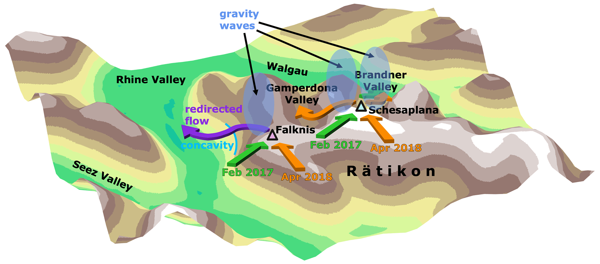
Figure 14Schematic illustration showing some of the key findings obtained in Sect. 4 when investigating the descent hotspot along the Rätikon.
-
Foehn descent occurs in distinct hotspots, often restricted to the immediate lee of mountain peaks and chains. The local terrain thus naturally anchors the regions of descending air parcels during foehn. Many of the hotspots are situated near the actual arrival locations of the foehn air parcels rather than in the vicinity of the Alpine crest. The well-known foehn valleys emerge as local descent maxima, and the overall most intense hotspot is located along the Rätikon range.
-
The elevation difference in the underlying terrain often provides an upper limit to the descent and is thus strongly correlated with its magnitude. Consequently, it reaches maximum values (exceeding 1500 m) in regions where the local peaks rank among the highest of the Alps and declines steeply on their downstream side, such as the Mont Blanc massif and the Bernese Alps. The time span of the descent, i.e., the time needed to cover a given descent segment, usually ranges between 4 to 10 min. However, locally the descent can occur even faster. The majority of air parcels descends approximately adiabatically and exhibits little change in specific humidity except for air parcels south of the Alpine crest, where evaporative cooling increases the specific humidity along the pathways of descending air parcels.
-
The strong descent within the Rhine Valley hotspot is associated with gravity waves excited by the peaks of the Rätikon, in particular the Falknis and the Schesaplana. On a local scale, the northwestern slope of the Falknis forms a topographic concavity that redirects the downslope flow towards the Rhine Valley floor near Vaduz (see also schematic illustration in Fig. 14). This westward deflection of the low-level flow consistently occurs during both events, independently of the impinging wind direction, but is more pronounced during the February 2017 event (see Fig. S9). In the lee of the Schesaplana, air parcels descend within a gravity wave and are guided into either the Brandner Valley or the Gamperdona Valley, depending on whether southwesterly or southeasterly winds impinge on the Rätikon (Fig. 14). Overall, the emerging gravity wave patterns vary for the different highlighted times, suggesting that no preferential wave regime is the most conducive for descent along the Rätikon. During February 2017, the gravity wave amplitudes generally increase in accordance with stronger lower- to mid-tropospheric winds within a stable layer above crest level. Additionally, key characteristics of hydraulic flow are discernible at certain times during this event. This observation suggests that density differences may indeed play a significant role in influencing the descent during these periods. In contrast, the temporal evolution of the descent activity during the April 2018 event demonstrates that nocturnal cooling and the resulting formation of a cold-air pool can impede strong descent of foehn air by elevating the level of neutral buoyancy for the descending air parcels and effectively attenuating the mountain waves.
Since the online trajectories explicitly resolve the rapid and small-scale downward motion in the lee of orography, our dataset enables us to follow the motion of air parcels as they cross the Alpine barrier. In contrast to previous qualitative and Eulerian approaches, the trajectory dataset therefore provides the opportunity to unequivocally identify descent hotspots and allows us to assess the foehn descent quantitatively and systematically using the Lagrangian perspective. Notably, our analysis encompasses a much broader region compared to existing studies, revealing that hotspots of foehn descent are not limited to the Rhine Valley and the Wipp Valley but exist across all foehn regions north of the Alps.
Even though we present the first systematic analysis of foehn descent employing a Lagrangian methodology, our study raises several questions to be addressed by prospective research. Firstly, it remains unclear what kind of gravity wave pattern (vertically propagating waves, breaking waves, trapped lee waves) coincides with the strongest descent. While different wave regimes could be detected within the hotspot region along the Rätikon, it is unknown whether these findings carry over to other descent hotspots and foehn events. One challenge when investigating the role of gravity waves in the descent lies in their characterization based on three-dimensional Eulerian fields. Here, we adopted a qualitative approach to describe the wave patterns at different time instants. In the future, a more quantitative approach (e.g., following Kruse and Smith, 2015) could elucidate the gravity wave characteristics during foehn more systematically.
In addition, although our study highlights the importance of gravity waves for the descent of foehn air, we did not explicitly disentangle the importance of the different mechanisms (see also Sect. 5.3). For instance, previous studies have suggested that density differences between two air mass reservoirs, separated by an orographic barrier, are the cause for the descent (e.g., Mayr and Armi, 2008; Armi and Mayr, 2011). The online trajectories could serve as an appropriate dataset to partition the descent into a buoyancy-driven fraction and a wave-driven fraction, provided that these two mechanisms can be clearly separated using a Lagrangian momentum budget. Future endeavors should thus focus on determining the physical mechanisms that cause the descending motion. Our extensive Lagrangian dataset, including the diagnosed descent locations, is a promising foundation for such investigations.
Highlighting the relevance of potential temperature differences between the descending air and the valley atmosphere, the case study of April 2018 illustrates that nocturnal cold-air-pool formation can produce a smooth virtual topography. This, in turn, inhibits strong descent by elevating the level of neutral buoyancy and effectively dampening the amplitude of gravity waves. Still, further in-depth analysis is required to corroborate the significance of this effect on the descent. Besides the diurnal cycle, other factors might influence the descent of foehn air parcels as well. In this regard, the upstream flow splitting at the junction of the Rhine Valley and the Seez Valley has been mentioned by a previous study (Zängl et al., 2004a). While we did not find a clear correlation between the flow splitting and the descent activity along the Rätikon, future studies are necessary to clarify the effect of the flow splitting on the descent.
In conclusion, the present paper provides new insights into one of the long-standing conundrums in foehn research. Using online trajectories, we have examined the descent of foehn air parcels from an unprecedented Lagrangian perspective. This methodology enabled us to investigate the phenomenon quantitatively and along the entire Alpine arc. Nevertheless, numerous open questions still remain unanswered, for instance regarding the importance of the different mechanisms or the transferability of our findings to other hotspot regions, emphasizing the need for further research. Our extensive trajectory dataset offers an opportunity to tackle these questions.
A1 Specifics of the model setup
Table A1Overview of the 15 foehn events that have been simulated with the COSMO model. The foehn types are determined following Jansing et al. (2022).
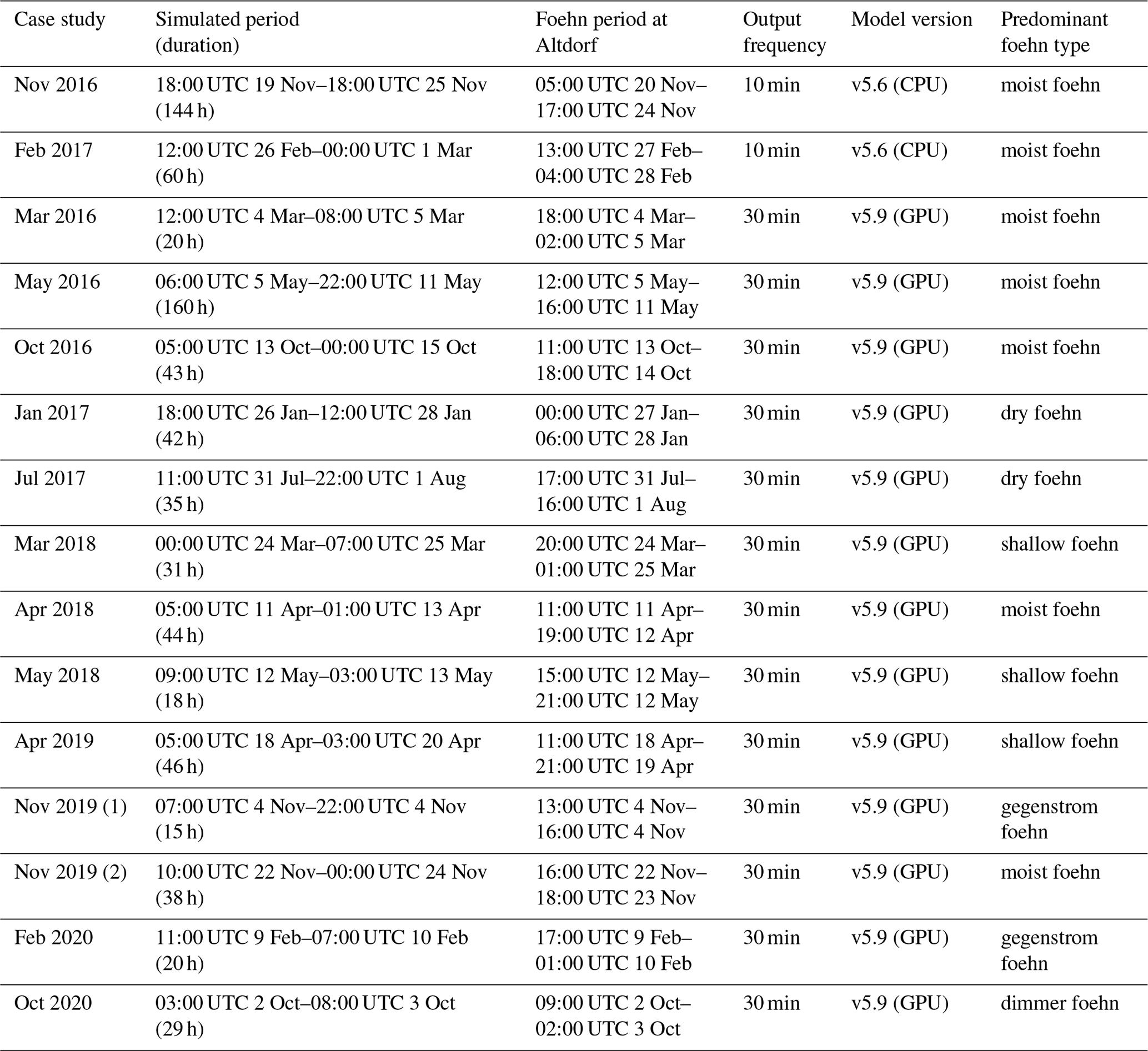
Using a climatology of different foehn types in the 5-year period from November 2015 to November 2020 (Jansing et al., 2022), we selected 13 events that represent all seasons and different foehn types (Table A1) and calculated hindcasts for each of these. The 13 events are complemented by two additional simulations that were performed at an earlier stage (the November 2016 and February 2017 events) with the goal of a more detailed analysis (see also Jansing and Sprenger, 2022, for the November 2016 event). Therefore, the simulated periods for these two events have been extended compared to the actual foehn period at Altdorf (see Table A1). Furthermore, the March 2018 case study also ran for a longer period in order to extend the simulated period of this particular shallow-foehn event (see also Jansing, 2023), which lasted only for a short period in Altdorf but longer at other foehn stations closer to the Alpine crest.
Table A2Overview of the online trajectory setups for the 15 foehn events.
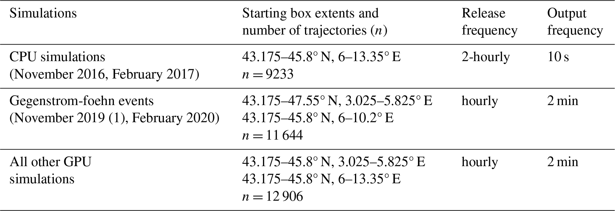
For November 2016 and February 2017, output is written to disk at a higher temporal resolution (10 min). While the November 2016 and February 2017 events have been simulated with COSMO version 5.6 on central processing units (CPUs), the other case studies made use of the GPU capability of both the COSMO model and the online trajectory module. Porting the existing online trajectory module to GPUs (see also Bukenberger et al., 2023) substantially enhanced the performance of the new model setup and allowed us to conduct an extended number of simulations with COSMO version 5.9. Aside from these differences in the model version, the simulations were performed with virtually identical setups, except for minor changes in a tuning parameter and the soil model, to align the GPU runs with the latest operational setup of MeteoSwiss.
A2 Specifics of the online trajectory setup
Here, we provide additional details on the exact setup of the online trajectory module. For all simulations, the spacing between starting points has been set to 0.175° and 250 m in the horizontal and vertical, respectively. The lowest trajectories were released 20 , reaching up to a maximum of 5 In a tradeoff between the largest possible distance to the Alpine arc while nevertheless taking into account all potential source regions for foehn air parcels, the trajectory starting points were cropped by a polygon with 50 km distance (violet contours in Fig. 1b and c) to the innermost closed 1500 m contour (blue contours in Fig. 1b and c) around the Alps (the same as in Jansing and Sprenger, 2022).
Air parcels were released in 2-hourly time intervals for the November 2016 and February 2017 case studies and in hourly time intervals for all other case studies (Table A2). The trajectory calculations started upon initialization of the model and ended 8 h prior to the end of the simulated period. For the February 2017 case study, trajectories were only released until 18 h prior to the end of the simulated period, as the foehn period was considerably shorter compared to the simulated period for this event. Each trajectory was calculated until reaching a maximum length of 36 h. All standard prognostic variables were traced along the trajectories. For the November 2016 and February 2017 events, output was written at the highest possible temporal resolution (10 s). For all other case studies, the trajectory output was stored in 2 min steps. Therefore, to homogenize the trajectory dataset, the temporal resolutions of the trajectory data from November 2016 and February 2017 were coarse-grained to 2 min for this study.
Note that the applied selection procedure to obtain foehn trajectories (Sect. 2.2) results in a substantially varying total number of selected trajectories between the cases studied (Fig. S1 in the Supplement), ranging from more than 105 to less than 102 trajectories (for the March 2018 case). This can have several different reasons. First of all, longer simulation periods, as for example for November 2016 or May 2016, will automatically result in a larger number of foehn trajectories, as more trajectories are released in total. Secondly, all events with a total of less than 103 trajectories belong to the shallow-foehn type (March 2018, May 2018) or the gegenstrom-foehn type (November 2019 (1), February 2020; see also Jansing, 2023). For these foehn types, defining a feasible starting setup is challenging. The weak large-scale flow during shallow foehn would require the start of trajectories closer to the Alpine crest so that more of them are able to reach the northern foehn regions. The pronounced zonal flow above crest level during gegenstrom foehn, in turn, requires starting points to be positioned more to the west rather than to the south. Although the starting setup has been adjusted for the gegenstrom-foehn events (Fig. 1c), it is apparently still challenging to capture the pathways of foehn air parcels during these events. The selection procedure requires a trajectory to intersect with the Alpine crest line, which might be a too-rigid criterion for many trajectories during gegenstrom foehn, as they approach the foehn regions from the west (with some exceptions). Finally, the foehn flow in the model might also be too weak during the simulations, preventing a larger number of trajectories from descending into the northern foehn regions. Despite this wide range in the number of trajectories per case, we decided to retain all events for the analyses, as the trajectory dataset is in any case collectively analyzed in large parts of the paper. Note that the presented case studies (February 2017, April 2019; see Sect. 4) in particular feature a reasonably large number of foehn trajectories to be investigated with further scrutiny (Fig. S1).
Operational COSMO-1 analyses are available for research purposes upon request to MeteoSwiss. Processed data from the simulations are available from the authors upon request. The code used for the analysis and visualization is written in Python 3.9 and is available from the authors upon request.
The supplement related to this article is available online at: https://doi.org/10.5194/wcd-5-463-2024-supplement.
All co-authors equally contributed to the design of the study and the interpretation of the results. LJ conducted the numerical simulations, processed the data, performed the analysis, and prepared the figures in the context of his PhD project. LJ wrote the paper, supported by MS and LP.
At least one of the (co-)authors is a member of the editorial board of Weather and Climate Dynamics. The peer-review process was guided by an independent editor, and the authors also have no other competing interests to declare.
Publisher's note: Copernicus Publications remains neutral with regard to jurisdictional claims made in the text, published maps, institutional affiliations, or any other geographical representation in this paper. While Copernicus Publications makes every effort to include appropriate place names, the final responsibility lies with the authors.
We acknowledge the Swiss National Supercomputing Centre for providing access to the computational resources. Two of the simulations (November 2016, February 2017) were conducted within the development project d111/d111m, and the remaining simulations were performed using resources of the s1063 project. In this regard, we want to express our thanks to Sebastian Schemm for providing access to the resources of s1063. Furthermore, we acknowledge the Federal Office of Meteorology and Climatology MeteoSwiss for giving us access to the COSMO-1 analysis data, which were used as initial and boundary conditions for the simulations. Additionally, we are grateful for the technical help of Annette Miltenberger and Annika Oertel in setting up the initial version of the online trajectory module. Stefan Rüdisühli, Katie Osterried, and Sebastian Schemm are acknowledged for guiding the GPU porting of the online trajectory module. Moreover, we express our gratitude to Heini Wernli for the valuable input. Finally, we appreciate the efforts of the two reviewers. One of the reviewers deserves special recognition, as the reviewer's feedback and many suggestions helped to significantly improve an earlier version of the manuscript.
This research has been supported by the Schweizerischer Nationalfonds zur Förderung der Wissenschaftlichen Forschung (grant no. 181992).
This paper was edited by Silvio Davolio and reviewed by Georg Mayr and one anonymous referee.
Armi, L. and Mayr, G. J.: Continuously stratified flows across an Alpine crest with a pass: Shallow and deep föhn, Q. J. Roy. Meteor. Soc., 133, 459–477, https://doi.org/10.1002/qj.22, 2007. a, b
Armi, L. and Mayr, G. J.: The descending stratified flow and internal hydraulic jump in the lee of the Sierras, J. Appl. Meteorol. Clim., 50, 1995–2011, https://doi.org/10.1175/JAMC-D-10-05005.1, 2011. a, b, c, d
Armi, L. and Mayr, G. J.: Virtual and real topography for flows across mountain ranges, J. Appl. Meteorol. Clim., 54, 723–731, https://doi.org/10.1175/JAMC-D-14-0231.1, 2015. a, b, c, d, e, f
Baldauf, M. and Zängl, G.: Horizontal nonlinear Smagorinsky diffusion, COSMO Newsletter 12, Deutscher Wetterdienst, http://www.cosmo-model.org/content/model/documentation/newsLetters/newsLetter12/1-baldauf.pdf (last access: 21 March 2024), 2012. a
Baldauf, M., Seifert, A., Förstner, J., Majewski, D., Raschendorfer, M., and Reinhardt, T.: Operational convective-scale numerical weather prediction with the COSMO model: Description and sensitivities, Mon. Weather Rev., 139, 3887–3905, https://doi.org/10.1175/MWR-D-10-05013.1, 2011. a
Baumann, K., Maurer, H., Rau, G., Piringer, M., Pechinger, U., Prévôt, A., Furger, M., Neininger, B., and Pellegrini, U.: The influence of south Foehn on the ozone distribution in the Alpine Rhine Valley–results from the MAP field phase, Atmos. Environ., 35, 6379–6390, https://doi.org/10.1016/S1352-2310(01)00364-8, 2001. a
Billwiller, R.: Besprechung von M. F. F. Hébert's “Etude sur les grands mouvements de l'atmosphère et sur le Foehn et le Scirocco pendant l'hiver 1876/77”, Z. Oester. Ges. Meteorol., 13, 317–320, 1878. a
Blumen, W.: Mountain meteorology, in: Atmospheric processes over complex terrain, edited by: Blumen, W., American Meteorological Society, Boston, MA, https://doi.org/10.1007/978-1-935704-25-6_1, pp. 1–4, 1990. a
Bougeault, P., Binder, P., Buzzi, A., Dirks, R., Houze, R., Kuettner, J., Smith, R. B., Steinacker, R., and Volkert, H.: The MAP special observing period, B. Am. Meteorol. Soc., 82, 433–462, https://doi.org/10.1175/1520-0477(2001)082<0433:TMSOP>2.3.CO;2, 2001. a
Bukenberger, M., Rüdisühli, S., and Schemm, S.: Jet stream dynamics from a PV gradient perspective: The method and its application to a km-scale simulation, Q. J. Roy. Meteor. Soc., 149, 2409–2432, https://doi.org/10.1002/qj.4513, 2023. a
Clark, T. L. and Peltier, W.: On the evolution and stability of finite-amplitude mountain waves, J. Atmos. Sci., 34, 1715–1730, https://doi.org/10.1175/1520-0469(1977)034<1715:OTEASO>2.0.CO;2, 1977. a
Doms, G. and Baldauf, M.: A description of the nonhydrostatic regional COSMO-model – Part I: Dynamics and Numerics, Tech. rep., Deutscher Wetterdienst, https://doi.org/10.5676/DWD_pub/nwv/cosmo-doc_6.00_I, 2021. a, b
Drobinski, P., Haeberli, C., Richard, E., Lothon, M., Dabas, A., Flamant, P., Furger, M., and Steinacker, R.: Scale interaction processes during the MAP IOP 12 south föhn event in the Rhine Valley, Q. J. Roy. Meteor. Soc., 129, 729–753, https://doi.org/10.1256/qj.02.35, 2003. a
Drobinski, P., Steinacker, R., Richner, H., Baumann-Stanzer, K., Beffrey, G., Benech, B., Berger, H., Chimani, B., Dabas, A., Dorninger, M., Dürr, B., Flamant, C., Frioud, M., Furger, M., Gröhn, I., Gubser, S., Gutermann, T., Häberli, C., Häller- Scharnhost, E., Jaubert, G., Lothon, M., Mitev, V., Pechinger, U., Piringer, M., Ratheiser, M., Ruffieux, D., Seiz, G., Spatzierer, M., Tschannett, S., Vogt, S., Werner, R., and Zängl, G.: Föhn in the Rhine Valley during MAP: A review of its multiscale dynamics in complex valley geometry, Q. J. Roy. Meteor. Soc., 133, 897–916, https://doi.org/10.1002/qj.70, 2007. a
Dürr, B.: Automatisiertes Verfahren zur Bestimmung von Föhn in Alpentälern, Bundesamt für Meteorologie und Klimatologie, MeteoSchweiz, Arbeitsber. MeteoSchweiz, 223, 22 pp., https://www.meteoschweiz.admin.ch/dam/jcr:3ed2aec8-0901-417a-acc3-8be11cce440a/Foehnindex_Arbeitsbericht_223_Automatisiertes_Verfahren_zur_Bestimmung_von_Foehn_in_Alpentaelern_de.pdf (last access: 21 March 2024, 2008. a, b
Durran, D. R.: Mountain waves and downslope winds, in: Atmospheric processes over complex terrain, edited by: Blumen, W., American Meteorological Society, Boston, MA, 59–81, https://doi.org/10.1007/978-1-935704-25-6_4, 1990. a, b, c
Durran, D. R.: Mountain Meteorology | Lee Waves and Mountain Waves, in: Encyclopedia of Atmospheric Sciences, second edition, edited by: North, G. R., Pyle, J., and Zhang, F., Academic Press, Oxford, 95–102, https://doi.org/10.1016/B978-0-12-382225-3.00202-4, 2015. a
Elvidge, A. D. and Renfrew, I. A.: The causes of foehn warming in the lee of mountains, B. Am. Meteorol. Soc., 97, 455–466, https://doi.org/10.1175/BAMS-D-14-00194.1, 2016. a, b
Elvidge, A. D., Renfrew, I. A., King, J. C., Orr, A., and Lachlan-Cope, T. A.: Foehn warming distributions in nonlinear and linear flow regimes: A focus on the Antarctic Peninsula, Q. J. Roy. Meteor. Soc., 142, 618–631, https://doi.org/10.1002/qj.2489, 2014. a
Elvidge, A. D., Kuipers Munneke, P., King, J. C., Renfrew, I. A., and Gilbert, E.: Atmospheric drivers of melt on Larsen C Ice Shelf: Surface energy budget regimes and the impact of foehn, J. Geophys. Res.-Atmos., 125, e2020JD032463, https://doi.org/10.1029/2020JD032463, 2020. a, b
Ficker, H.: Warum steigt der Föhn in die Täler herab?, Meteorol. Z., 48, 227–229, 1931. a
Flamant, C., Drobinski, P., Nance, L., Banta, R., Darby, L., Dusek, J., Hardesty, M., Pelon, J., and Richard, E.: Gap flow in an Alpine valley during a shallow south föhn event: Observations, numerical simulations and hydraulic analogue, Q. J. Roy. Meteor. Soc., 128, 1173–1210, https://doi.org/10.1256/003590002320373256, 2002. a
Flamant, C., Drobinski, P., Furger, M., Chimani, B., Tschannett, S., Steinacker, R., Protat, A., Richner, H., Gubser, S., and Häberli, C.: Föohn/cold-pool interactions in the Rhine valley during MAP IOP 15, Q. J. Roy. Meteor. Soc., 132, 3035–3058, https://doi.org/10.1256/qj.06.36, 2006. a
Frey, K.: Beiträge zur Entwicklung des Föhns und Untersuchungen über Hochnebel, PhD thesis, Rentsch Söhne, Trimbach Olten, 1945. a
Fuhrer, O., Osuna, C., Lapillonne, X., Gysi, T., Cumming, B., Bianco, M., Arteaga, A., and Schulthess, T. C.: Towards a performance portable, architecture agnostic implementation strategy for weather and climate models, Supercomp. Front. Innov., 1, 45–62, https://doi.org/10.14529/jsfi140103, 2014. a
Gohm, A. and Mayr, G.: Hydraulic aspects of föhn winds in an Alpine valley, Q. J. Roy. Meteor. Soc., 130, 449–480, https://doi.org/10.1256/qj.03.28, 2004. a
Gohm, A., Zängl, G., and Mayr, G. J.: South foehn in the Wipp Valley on 24 October 1999 (MAP IOP 10): Verification of high-resolution numerical simulations with observations, Mon. Weather Rev., 132, 78–102, https://doi.org/10.1175/1520-0493(2004)132<0078:SFITWV>2.0.CO;2, 2004. a, b, c, d, e
Gubser, S.: Wechselwirkung zwischen Föhn und planetarer Grenzschicht, PhD thesis, ETH Zurich, https://doi.org/10.3929/ethz-a-005207902, 2006. a
Gutermann, T., Dürr, B., Richner, H., and Bader, S.: Föhnklimatologie Altdorf: Die lange Reihe (1864–2008) und ihre Weiterführung, Vergleich mit anderen Stationen, Arbeitsber. MeteoSchweiz, 241, 53 pp., Bundesamt für Meteorologie und Klimatologie, MeteoSchweiz, https://doi.org/10.3929/ethz-a-007583529, 2012. a, b, c
Haid, M., Gohm, A., Umek, L., Ward, H. C., Muschinski, T., Lehner, L., and Rotach, M. W.: Foehn–cold pool interactions in the Inn Valley during PIANO IOP2, Q. J. Roy. Meteor. Soc., 146, 1232–1263, https://doi.org/10.1002/qj.3735, 2020. a, b, c
Haid, M., Gohm, A., Umek, L., Ward, H. C., and Rotach, M. W.: Cold-air pool processes in the Inn Valley during föhn: A comparison of four cases during the PIANO campaign, Bound.-Lay. Meteorol., 182, 335–362, https://doi.org/10.1007/s10546-021-00663-9, 2022. a
Hann, J.: Zur Frage über den Ursprung des Föhn, Z. Oester. Ges. Meteorol., 1, 257–263, 1866. a
Heise, E., Ritter, B., and Schrodin, R.: Operational implementation of the multilayer soil model, COSMO tech. rep., Deutscher Wetterdienst, https://doi.org/10.5676/DWD_pub/nwv/cosmo-tr_9, 2006. a
Jackson, P., Mayr, G., and Vosper, S.: Dynamically-driven winds, chap. 3, in: Mountain Weather Research and Forecasting, edited by: Chow, F. K., De Wekker, S. F., and Snyder, B. J., Springer Atmospheric Sciences, 121–218, https://doi.org/10.1007/978-94-007-4098-3_3, 2013. a
Jansing, L.: A Lagrangian perspective on the Alpine Foehn, PhD thesis, ETH Zurich, https://doi.org/10.3929/ethz-b-000619589, 2023. a, b, c, d
Jansing, L. and Sprenger, M.: Thermodynamics and airstreams of a south foehn event in different Alpine valleys, Q. J. Roy. Meteor. Soc., 148, 2063–2085, https://doi.org/10.1002/qj.4285, 2022. a, b, c, d, e, f, g
Jansing, L., Papritz, L., Dürr, B., Gerstgrasser, D., and Sprenger, M.: Classification of Alpine south foehn based on 5 years of kilometre-scale analysis data, Weather Clim. Dynam., 3, 1113–1138, https://doi.org/10.5194/wcd-3-1113-2022, 2022. a, b, c, d, e
Jiang, Q., Doyle, J. D., and Smith, R. B.: Interaction between trapped waves and boundary layers, J. Atmos. Sci., 63, 617–633, https://doi.org/10.1175/JAS3640.1, 2006. a, b
Klemp, J. and Lilly, D.: The dynamics of wave-induced downslope winds, J. Atmos. Sci., 32, 320–339, https://doi.org/10.1175/1520-0469(1975)032<0320:TDOWID>2.0.CO;2, 1975. a
Kruse, C. G. and Smith, R. B.: Gravity wave diagnostics and characteristics in mesoscale fields, J. Atmos. Sci., 72, 4372–4392, https://doi.org/10.1175/JAS-D-15-0079.1, 2015. a
Kusaka, H., Nishi, A., Kakinuma, A., Doan, Q.-V., Onodera, T., and Endo, S.: Japan's south foehn on the Toyama Plain: Dynamical or thermodynamical mechanisms?, Int. J. Climatol., 41, 5350–5367, https://doi.org/10.1002/joc.7133, 2021. a, b, c
Lehmann, O.: Zur Geschichte der Föhntheorie, Vierteljahresschr. Naturforsch. Ges. Zürich, 82, 45–76, 1937. a
Lehner, M. and Rotach, M. W.: Current challenges in understanding and predicting transport and exchange in the atmosphere over mountainous terrain, Atmosphere, 9, 276, https://doi.org/10.3390/atmos9070276, 2018. a
Leuenberger, D., Koller, M., Fuhrer, O., and Schär, C.: A generalization of the SLEVE vertical coordinate, Mon. Weather Rev., 138, 3683–3689, https://doi.org/10.1175/2010MWR3307.1, 2010. a
Leutwyler, D., Fuhrer, O., Lapillonne, X., Lüthi, D., and Schär, C.: Towards European-scale convection-resolving climate simulations with GPUs: a study with COSMO 4.19, Geosci. Model Dev., 9, 3393–3412, https://doi.org/10.5194/gmd-9-3393-2016, 2016. a
Lezuo, T., Jansing, L., Rostkier-Edelstein, D., and Sprenger, M.: Is it foehn or sea breeze? Eulerian and Lagrangian analysis of the flow in the Jordan Valley, Meteorol. Z., 32, 367–381, https://doi.org/10.1127/metz/2023/1167, 2023. a
Mattingly, K. S., Mote, T. L., Fettweis, X., Van As, D., Van Tricht, K., Lhermitte, S., Pettersen, C., and Fausto, R. S.: Strong summer atmospheric rivers trigger Greenland Ice Sheet melt through spatially varying surface energy balance and cloud regimes, J. Climate, 33, 6809–6832, https://doi.org/10.1175/JCLI-D-19-0835.1, 2020. a
Mattingly, K. S., Turton, J. V., Wille, J. D., Noël, B., Fettweis, X., Rennermalm, Å. K., and Mote, T. L.: Increasing extreme melt in northeast Greenland linked to foehn winds and atmospheric rivers, Nat. Commun., 14, 1743, https://doi.org/10.1038/s41467-023-37434-8, 2023. a
Mayr, G. J. and Armi, L.: Föhn as a response to changing upstream and downstream air masses, Q. J. Roy. Meteor. Soc., 134, 1357–1369, https://doi.org/10.1002/qj.295, 2008. a, b, c, d, e
Mayr, G. J. and Armi, L.: The influence of downstream diurnal heating on the descent of flow across the Sierras, J. Appl. Meteorol. Clim., 49, 1906–1912, https://doi.org/10.1175/2010JAMC2516.1, 2010. a, b, c
Mayr, G. J., Armi, L., Gohm, A., Zängl, G., Durran, D. R., Flamant, C., Gaberšek, S., Mobbs, S., Ross, A., and Weissmann, M.: Gap flows: Results from the Mesoscale Alpine Programme, Q. J. Roy. Meteor. Soc., 133, 881–896, https://doi.org/10.1002/qj.66, 2007. a, b, c, d
Mellor, G. L. and Yamada, T.: Development of a turbulence closure model for geophysical fluid problems, Rev. Geophys., 20, 851–875, https://doi.org/10.1029/RG020i004p00851, 1982. a
Miltenberger, A. K., Pfahl, S., and Wernli, H.: An online trajectory module (version 1.0) for the nonhydrostatic numerical weather prediction model COSMO, Geosci. Model Dev., 6, 1989–2004, https://doi.org/10.5194/gmd-6-1989-2013, 2013. a, b
Miltenberger, A. K., Reynolds, S., and Sprenger, M.: Revisiting the latent heating contribution to foehn warming: Lagrangian analysis of two foehn events over the Swiss Alps, Q. J. Roy. Meteor. Soc., 142, 2194–2204, https://doi.org/10.1002/qj.2816, 2016. a, b
Mony, C.: Evaluating foehn development in a changing climate using machine learning and investigating the impact of foehn on forest fire occurrence and severity, Master's thesis, ETH Zurich, https://doi.org/10.3929/ethz-b-000594509, 2020. a
Muñoz, R. C., Armi, L., Rutllant, J. A., Falvey, M., Whiteman, C. D., Garreaud, R., Arriagada, A., Flores, F., and Donoso, N.: Raco wind at the exit of the Maipo Canyon in central Chile: climatology, special observations, and possible mechanisms, J. Appl. Meteorol. Clim., 59, 725–749, https://doi.org/10.1175/JAMC-D-19-0188.1, 2020. a
Pezzatti, G. B., De Angelis, A., and Conedera, M.: Potenzielle Entwicklung der Waldbrandgefahr im Klimawandel, chap. 3.8, in: Wald im Klimawandel. Grundlagen für Adaptationsstrategien, edited by: Pluess, A. R., Augustin, S., and Brang, P., Haupt, Bern, https://www.dora.lib4ri.ch/wsl/islandora/object/wsl:10619 (last access: 21 March 2024), pp. 223–246, 2016. a
Queney, P.: The problem of air flow over mountains: A summary of theoretical studies, B. Am. Meteorol. Soc., 29, 16–26, https://doi.org/10.1175/1520-0477-29.1.16, 1948. a
Raphael, M.: The Santa Ana winds of California, Earth Interact., 7, 1–13, https://doi.org/10.1175/1087-3562(2003)007<0001:TSAWOC>2.0.CO;2, 2003. a
Raschendorfer, M.: The new turbulence parameterization of LM, COSMO Newsletter 1, Deutscher Wetterdienst, https://www.cosmo-model.org/content/model/documentation/newsLetters/newsLetter01/newsLetter_01.pdf (last access: 21 March 2024), 2001. a
Reinhardt, T. and Seifert, A.: A three-category ice scheme for LMK, COSMO Newsletter 6, Deutscher Wetterdienst, https://www.cosmo-model.org/content/model/documentation/newsLetters/newsLetter06/cnl6_reinhardt.pdf (last access: 21 March 2024), 2006. a
Richner, H. and Hächler, P.: Understanding and forecasting Alpine foehn, chap. 4, in: Mountain Weather Research and Forecasting, edited by: Chow, F. K., De Wekker, S. F., and Snyder, B. J., Springer Atmospheric Sciences, 219–260, https://doi.org/10.1007/978-94-007-4098-3_4, 2013. a, b, c, d
Richner, H., Dürr, B., Gutermann, T., and Bader, S.: The use of automatic station data for continuing the long time series (1864 to 2008) of foehn in Altdorf, Meteorol. Z., 23, 159–166, https://doi.org/10.1127/0941-2948/2014/0528, 2014. a
Ritter, B. and Geleyn, J.-F.: A comprehensive radiation scheme for numerical weather prediction models with potential applications in climate simulations, Mon. Weather Rev., 120, 303–325, https://doi.org/10.1175/1520-0493(1992)120<0303:ACRSFN>2.0.CO;2, 1992. a
Rossmann, F.: Über das Absteigen des Föhns in die Täler, Ber. deutsch. Wetterd. US-Zone, 12, 94–98, 1950. a
Rotach, M. W., Wohlfahrt, G., Hansel, A., Reif, M., Wagner, J., and Gohm, A.: The world is not flat: Implications for the global carbon balance, B. Am. Meteorol. Soc., 95, 1021–1028, https://doi.org/10.1175/BAMS-D-13-00109.1, 2014. a
Saigger, M. and Gohm, A.: Is it north or west foehn? A Lagrangian analysis of Penetration and Interruption of Alpine Foehn intensive observation period 1 (PIANO IOP 1), Weather Clim. Dynam., 3, 279–303, https://doi.org/10.5194/wcd-3-279-2022, 2022. a, b, c, d
Schär, C., Leuenberger, D., Fuhrer, O., Lüthi, D., and Girard, C.: A new terrain-following vertical coordinate formulation for atmospheric prediction models, Mon. Weather Rev., 130, 2459–2480, https://doi.org/10.1175/1520-0493(2002)130<2459:ANTFVC>2.0.CO;2, 2002. a
Schättler, U., Doms, G., and Schraff, C.: A description of the nonhydrostatic regional COSMO-model – Part VII: User's Guide, Tech. rep., Deutscher Wetterdienst, https://doi.org/10.5676/DWD_pub/nwv/cosmo-doc_6.00_VII, 2021. a
Schweitzer, H.: Versuch einer Erklärung des Föhns als Luftströmung mit überkritischer Geschwindigkeit, Arch. Meteorol. Geophys. Bioklim., 5, 350–371, https://doi.org/10.1007/BF02247776, 1952. a
Schüepp, W.: Die qualitative und quantitative Bedeutung der Föhnmauer, Meteorol. Rundsch., 5, 136–138, 1952. a
Seibert, P., Feldmann, H., Neininger, B., Bäumle, M., and Trickl, T.: South foehn and ozone in the Eastern Alps – case study and climatological aspects, Atmos. Environ., 34, 1379–1394, https://doi.org/10.1016/S1352-2310(99)00439-2, 2000. a
Smith, R. B.: The influence of mountains on the atmosphere, Adv. Geophys., 21, 87–230, https://doi.org/10.1016/S0065-2687(08)60262-9, 1979. a
Sprenger, M., Dürr, B., and Richner, H.: Foehn studies in Switzerland, chap. 11, in: From weather observations to atmospheric and climate sciences in Switzerland, edited by: Willemse, S. and Furger, M., vdf Hochschulverlag AG, Zurich, 215–248, https://doi.org/10.3218/3746-3, 2016. a, b, c
Steinacker, R.: Alpiner Föhn – eine neue Strophe zu einem alten Lied, Promet, 32, 3–10, 2006. a, b, c
Steinacker, R., Spatzierer, M., Dorninger, M., and Häberli, C.: Selected results of the FORMAT field measurements, Österr. Beitr. Meteorol. Geophys., 29, 55–70, 2003. a
Steppeler, J., Doms, G., Schättler, U., Bitzer, H. W., Gassmann, A., Damrath, U., and Gregoric, G.: Meso-gamma scale forecasts using the nonhydrostatic model LM, Meteorol. Atmos. Phys., 82, 75–96, https://doi.org/10.1007/s00703-001-0592-9, 2003. a
Strauss, S.: An ill wind: the Foehn in Leukerbad and beyond, J. Roy. Anthropol. Inst., 13, S165–S181, https://doi.org/10.1111/j.1467-9655.2007.00406.x, 2007. a
Streiff-Becker, R.: Altes und Neues über den Glarner-Föhn, Mitt. Naturforsch. Ges. Kt. Glarus, 52 pp., 1930. a, b
Stucki, P., Brönnimann, S., Martius, O., Welker, C., Rickli, R., Dierer, S., Bresch, D. N., Compo, G. P., and Sardeshmukh, P. D.: Dynamical downscaling and loss modeling for the reconstruction of historical weather extremes and their impacts: A severe foehn storm in 1925, B. Am. Meteorol. Soc., 96, 1233–1241, https://doi.org/10.1175/BAMS-D-14-00041.1, 2015. a
Umek, L., Gohm, A., Haid, M., Ward, H. C., and Rotach, M. W.: Large-eddy simulation of foehn–cold pool interactions in the Inn Valley during PIANO IOP 2, Q. J. Roy. Meteor. Soc., 147, 944–982, https://doi.org/10.1002/qj.3954, 2021. a, b
Umek, L., Gohm, A., Haid, M., Ward, H. C., and Rotach, M. W.: Influence of grid resolution of large-eddy simulations on foehn-cold pool interaction, Q. J. Roy. Meteor. Soc., 148, 1840–1863, https://doi.org/10.1002/qj.4281, 2022. a
Vergara-Temprado, J., Ban, N., Panosetti, D., Schlemmer, L., and Schär, C.: Climate models permit convection at much coarser resolutions than previously considered, J. Climate, 33, 1915–1933, https://doi.org/10.1175/JCLI-D-19-0286.1, 2020. a
Vosper, S. B., Ross, A. N., Renfrew, I. A., Sheridan, P., Elvidge, A. D., and Grubišić, V.: Current challenges in orographic flow dynamics: turbulent exchange due to low-level gravity-wave processes, Atmosphere, 9, 361, https://doi.org/10.3390/atmos9090361, 2018. a
Wastl, C., Schunk, C., Lüpke, M., Cocca, G., Conedera, M., Valese, E., and Menzel, A.: Large-scale weather types, forest fire danger, and wildfire occurrence in the Alps, Agr. Forest Meteorol., 168, 15–25, https://doi.org/10.1016/j.agrformet.2012.08.011, 2013. a
Wicker, L. J. and Skamarock, W. C.: Time-splitting methods for elastic models using forward time schemes, Mon. Weather Rev., 130, 2088–2097, https://doi.org/10.1175/1520-0493(2002)130<2088:TSMFEM>2.0.CO;2, 2002. a
Wild, H.: Über Föhn und Eiszeit. Mit Nachtrag: Der Schweizer-Föhn, Jent & Reinert, 1868. a
Xue, M.: High-order monotonic numerical diffusion and smoothing, Mon. Weather Rev., 128, 2853–2864, https://doi.org/10.1175/1520-0493(2000)128<2853:HOMNDA>2.0.CO;2, 2000. a
Zängl, G.: Deep and shallow south foehn in the region of Innsbruck: Typical features and semi-idealized numerical simulations, Meteorol. Atmos. Phys., 83, 237–261, https://doi.org/10.1007/s00703-002-0565-7, 2003. a
Zängl, G.: North foehn in the Austrian Inn Valley: A case study and idealized numerical simulations, Meteorol. Atmos. Phys., 91, 85–105, https://doi.org/10.1007/s00703-004-0106-7, 2006. a, b
Zängl, G. and Hornsteiner, M.: Can trapped gravity waves be relevant for severe foehn windstorms? A case study, Meteorol. Z., 16, 203–212, https://doi.org/10.1127/0941-2948/2007/0199, 2007. a, b
Zängl, G., Chimani, B., and Häberli, C.: Numerical simulations of the foehn in the Rhine Valley on 24 October 1999 (MAP IOP 10), Mon. Weather Rev., 132, 368–389, https://doi.org/10.1175/1520-0493(2004)132<0368:NSOTFI>2.0.CO;2, 2004a. a, b, c, d, e, f, g, h, i, j, k
Zängl, G., Gohm, A., and Geier, G.: South foehn in the Wipp Valley – Innsbruck region: Numerical simulations of the 24 October 1999 case (MAP-IOP 10), Meteorol. Atmos. Phys., 86, 213–243, https://doi.org/10.1007/s00703-003-0029-8, 2004b. a, b, c, d, e
Zou, X., Bromwich, D. H., Montenegro, A., Wang, S.-H., and Bai, L.: Major surface melting over the Ross Ice Shelf part I: Foehn effect, Q. J. Roy. Meteor. Soc., 147, 2874–2894, https://doi.org/10.1002/qj.4104, 2021. a
Zumbrunnen, T., Bugmann, H., Conedera, M., and Bürgi, M.: Linking forest fire regimes and climate–a historical analysis in a dry inner Alpine valley, Ecosystems, 12, 73–86, https://doi.org/10.1007/s10021-008-9207-3, 2009. a
The sensitivity with respect to the thresholds in altitude and time has been tested (Fig. S4 in the Supplement). See Sect. 3.1 for further details.
The February 2017 event was simulated over an extended time period (see Appendix A1 and Table A1). Therefore, a longer period prior to and after the foehn episode was captured by the simulation compared to other events. In the context of the case studies, the different time instants are given in hours since the event start, whereas the event start and end are defined by the simulated period.
- Abstract
- Introduction
- Data and methods
- Characteristics of foehn descent on the Alpine scale
- The descent of foehn air parcels into the Rhine Valley
- Discussion
- Conclusions
- Appendix A: Details on the COSMO model setup
- Code and data availability
- Author contributions
- Competing interests
- Disclaimer
- Acknowledgements
- Financial support
- Review statement
- References
- Supplement