Influence of radiosonde observations on the sharpness and altitude of the midlatitude tropopause in the ECMWF IFS

Initial conditions of current numerical weather prediction systems insufficiently represent the sharp vertical gradients across the midlatitude tropopause. Data assimilation may provide a means to improve tropopause structure by correcting the erroneous background forecast towards the observations. In this paper, the influence of assimilating radiosonde observations on tropopause structure, i.e., the sharpness and altitude, is investigated in the ECMWF's Integrated Forecasting System. We evaluate 9729 midlatitude radiosondes launched during 1 month in autumn 2016. About 500 of these radiosondes, launched on request during the North Atlantic Waveguide Downstream Impact Experiment (NAWDEX) field campaign, are used to set up an observing system experiment (OSE) that comprises two assimilation forecast experiments, one run with and one without the non-operational soundings. The influence on the tropopause is assessed in a statistical, tropopause-relative evaluation of observation departures of temperature, static stability (N²), wind speed, and wind shear from the background forecast and the analysis. Temperature is overestimated by the background at the tropopause (warm bias, ∼ 1 K) and underestimated in the lower stratosphere (cold bias, −0.3 K) leading to an underestimation of the abrupt increase in N² at the tropopause. The increments (differences in analysis and background) reduce these background biases and improve tropopause sharpness. Profiles with sharper tropopause exhibit stronger background biases but also an increased positive influence of the observations on temperature and N² in the analysis. Wind speed is underestimated in the background, especially in the upper troposphere (∼ 1 m s⁻¹), but the assimilation improves the wind profile. For the strongest winds the background bias is roughly halved. The positive influence on the analysis wind profile is associated with an improved vertical distribution of wind shear, particularly in the lower stratosphere. We furthermore detect a shift in the analysis tropopause altitude towards the observations. The evaluation of the OSE highlights that the diagnosed tropopause sharpening can be primarily attributed to the radiosondes. This study shows that data assimilation improves wind and temperature gradients across the tropopause, but the sharpening is small compared with the model biases. Hence, the analysis still systematically underestimates tropopause sharpness which may negatively impact weather and climate forecasts.

1 Introduction

The extratropical tropopause is the physical boundary that separates the well-mixed upper troposphere (UT) from the stably stratified lower stratosphere (LS) (e.g., Gettelman et al., 2011). The transition from the UT to the LS is characterized by sharp vertical gradients of temperature, humidity, and wind, and the strength of these gradients determines the sharpness and altitude of the tropopause. In the UT, the average temperature decreases with altitude towards a minimum at the tropopause. Above the tropopause, an ∼ 2 km thick temperature inversion is typically followed by a nearly isothermal temperature in the LS. This temperature distribution leads to a rapid increase in the squared static stability (N²) from low values (1 × 10⁻⁴ s⁻²) in the UT to high values (4 × 10⁻⁴ s⁻²) in the lowermost 2–3 km of the LS referred to as the tropopause inversion layer (TIL; Birner et al., 2002). The N² maximum above the tropopause (within the TIL) is used as a metric for tropopause sharpness (e.g., Haualand and Spengler, 2021; Boljka and Birner, 2022). The TIL acts as a barrier for vertical transport leading to sharp gradients of trace species across the tropopause, e.g., of specific humidity (Krüger et al., 2022). The vertical distribution of wind in the midlatitude UTLS is highly variable, but on average wind speed linearly increases with altitude in the troposphere towards a maximum just below the tropopause (e.g., Birner et al., 2002; Birner, 2006; Schäfler et al., 2020). Above the tropopause, wind speed rapidly decreases with altitude in the LS associated with an increased magnitude of vertical shear of the horizontal wind (Birner, 2006; Schäfler et al., 2020).

Temperature and wind gradients directly determine the potential vorticity (PV) distribution. The strong meridional PV gradient near the tropopause acts as a waveguide for Rossby waves (Schwierz et al., 2004; Martius et al., 2010) and, in turn, impacts downstream weather development in the midlatitudes (Harvey et al., 2018). Thus, an accurate representation of the sharp cross-tropopause gradients in the initial conditions may be of high importance for numerical weather prediction (NWP) models. However, forecast PV gradients rapidly decline within short (12–24 h) lead times (Gray et al., 2014; Lavers et al., 2023) which is attributed to a smoothing effect of the advection scheme that dominates sharpening effects of parameterized processes such as radiative cooling driven by water vapor, microphysics, and turbulent mixing (Saffin et al., 2017). The weakening PV gradients are likely associated with background forecast errors of temperature, humidity, and wind at the tropopause, which may affect the quality of the analysis.

At the tropopause, Bland et al. (2021) found a warm bias (a few tenths of 1 K) in analyses of the European Centre for Medium-Range Weather Forecast's (ECMWF) Integrated Forecasting System (IFS). The presence of a warm bias in IFS short-range forecasts and analyses near the tropopause was also indicated in earlier studies (Bonavita, 2014; Ingleby et al., 2016). In the LS, a moist bias (e.g., Krüger et al., 2022) leads to a cold bias at altitudes between 0.5 and 2 km above the tropopause in the IFS (Bland et al., 2021). Schäfler et al. (2020) indicated a systematic underestimation of jet stream wind maxima and showed large wind errors of up to 10 m s⁻¹ for individual cases in IFS short-range forecasts and analyses. Lavers et al. (2023) detected a vertically increasing slow wind bias (up to roughly 0.6 m s⁻¹) in the troposphere in the IFS background. In agreement with the wind errors, quantitative assessments of the magnitude of vertical wind shear at the tropopause revealed an underestimation by a factor of 2–5 (Houchi et al., 2010; Schäfler et al., 2020).

Data assimilation (DA) has shown a positive influence on the analysis in the UTLS, i.e., a reduction in the short-range forecast errors of temperature (e.g., Radnóti et al., 2010; Bonavita, 2014) and wind (e.g., Weissmann and Cardinali, 2007; Weissmann et al., 2012; Lavers et al., 2023; Martin et al., 2023). Two dedicated studies elaborated the influence of DA on tropopause sharpness (Birner et al., 2006; Pilch Kedziersky et al., 2016). Birner et al. (2006) investigated the role of satellite DA in the Canadian Middle Atmosphere Model (CMAM), providing a vertical resolution of 1 km near the tropopause, and used a 3DVAR assimilation scheme. A decrease in $N_{max}^{\mathrm{2}}$ in an experiment with assimilated satellite observations compared with a model run without satellite observations suggested that satellite DA smears out the gradients near the tropopause. The more recent study by Pilch Kedziersky et al. (2016) analyzed the influence on tropopause sharpness at the positions of GPS radio occultation (GPS RO) observations in ECMWF's ERA–Interim reanalysis and IFS analysis, using 4DVAR (e.g., Rabier et al., 2000) and a vertical resolution of ∼ 500 m at the tropopause. The detected increase in N² in an ∼ 1 km-thick layer just above the tropopause and a decrease in N² above and below this layer corresponds to a tropopause sharpening, which was attributed to the assimilation of GPS RO data. GPS RO data have a higher vertical resolution compared with radiance data from near-nadir sounders (e.g., Bonavita, 2014, and references therein), which provide the vast majority of all data assimilated in the IFS (e.g., Pauley and Ingleby, 2022). Both studies, which show different effects of DA on tropopause sharpness, differ in terms of the applied methods to diagnose the influence, the used observation type, the spatial resolution, and the DA schemes. It should also be noted that both studies are based on variational DA schemes without a flow-dependent estimate of the error covariance matrix (B). Flow-dependent estimates of B as they are nowadays used in the hybrid DA scheme of ECMWF are expected to lead to more accurate increment structures and therefore a better representation of sharp gradients.

Radiosondes provide highly resolved and accurate profiles of temperature and wind components (e.g., Vaisala, 2017), and thus are suitable to resolve the sharp vertical gradients at the tropopause. The measured quantities are directly assimilated and, although they only account for a small proportion (about 2 %) of the total assimilated meteorological information, they contribute to a 5 % reduction in 24 h forecast error in the ECMWF IFS in a statistical sense (Pauley and Ingleby, 2022). In addition, radiosondes serve as anchor observations for the variational bias correction, e.g., for satellite observations, highlighting their important role for DA (Cucurull and Anthes, 2014). The impact of individual observation capabilities, such as radiosondes, is typically assessed by performing observing system experiments (OSEs; e.g., Bonavita, 2014), e.g., during special observation periods related to field campaigns (e.g., Weissmann et al., 2012; Schindler et al., 2020; Borne et al., 2023). The DA impact can be studied either in model space by using 3D gridded model output or in observation space, which is the 4DVAR model output (observations and departures) representative for the position and time of the assimilated observation. The latter method has the advantage that a comparison of the observations and departures allows the influence of individual measurement types and parameters in the NWP system to be evaluated.

In this study, we further address the question of whether DA sharpens or smoothens the near-tropopause gradients. The aim is to quantify the change in tropopause structure from the first guess to the analysis and to relate it to the assimilation of radiosondes. For this purpose, we make use of the 1-month campaign period of the North Atlantic Waveguide Downstream Impact Experiment (NAWDEX; Schäfler et al., 2018) in autumn 2016 during which 9729 radiosonde profiles in a region between eastern North America and Europe were assimilated. Of the 9729 radiosondes, 497 were non-operationally launched and their impact was studied as an OSE, which consists of two cycled IFS runs, one with and one without the additional observations (Schindler et al., 2020). The statistical evaluation is performed in a tropopause-relative framework which is mandatory to preserve the outlined sharp gradients in the UTLS when averaging profiles with different tropopause altitudes (Birner, 2006). As no humidity data at and above the tropopause are assimilated (Bland et al., 2021), we restrict the analysis to profile observations of temperature and wind. We address the following specific research questions:

1. How is tropopause sharpness represented in background forecasts and what is the influence of DA on the analysis? Does the diagnosed influence on temperature and wind depend on tropopause structure and vary in different dynamic situations?

2. Does the influence on the temperature profile affect tropopause altitude?

3. Can the diagnosed influence be attributed to the assimilated radiosondes or do other observations also affect tropopause structure?

2 Data and methods

2.1 Description of the data set and the OSE

In this study, we analyze about 9200 radiosonde profiles (Fig. 1a) that were routinely measured at 581 sites covering a wide area between North America and Europe from the subtropics to high latitudes (30–85° N, 95° W–30° E) during a 1-month autumn period (17 September to 18 October 2016). The majority of these observations (96 %) were performed at 200 land-based stations while the minor share (4 %) were ship-based observations at 381 variable positions across the North Atlantic. In addition to the routine profile observations, about 500 extra radiosondes were launched in the course of the NAWDEX field campaign (Fig. 1b), which had the aim to better explore the influence of diabatic processes on the polar jet and weather downstream (Schäfler et al., 2018). Over Europe the extra, on-demand radiosondes were released in a variety of synoptic situations, for instance, in diabatically active warm conveyor belt flows associated with cyclones or in upper-level ridges associated with blocking situations. Six stations over Canada, upstream of the NAWDEX operation region, released two additional radiosondes per day. In addition to the radiosonde observations, more than 700 dropsondes were released from research aircraft during the NAWDEX period (mostly in the subtropical and tropical west Atlantic; see Schindler et al., 2020). Due to the low data coverage of the dropsondes above and at the tropopause related to the limited flight altitude of the aircraft, we restrict our analysis to the radiosonde profiles. All radiosonde and dropsonde profiles were made available for operational assimilation at weather centers (Schäfler et al., 2018). Figure 1 shows the launching position of those radiosondes that were assimilated within the IFS.

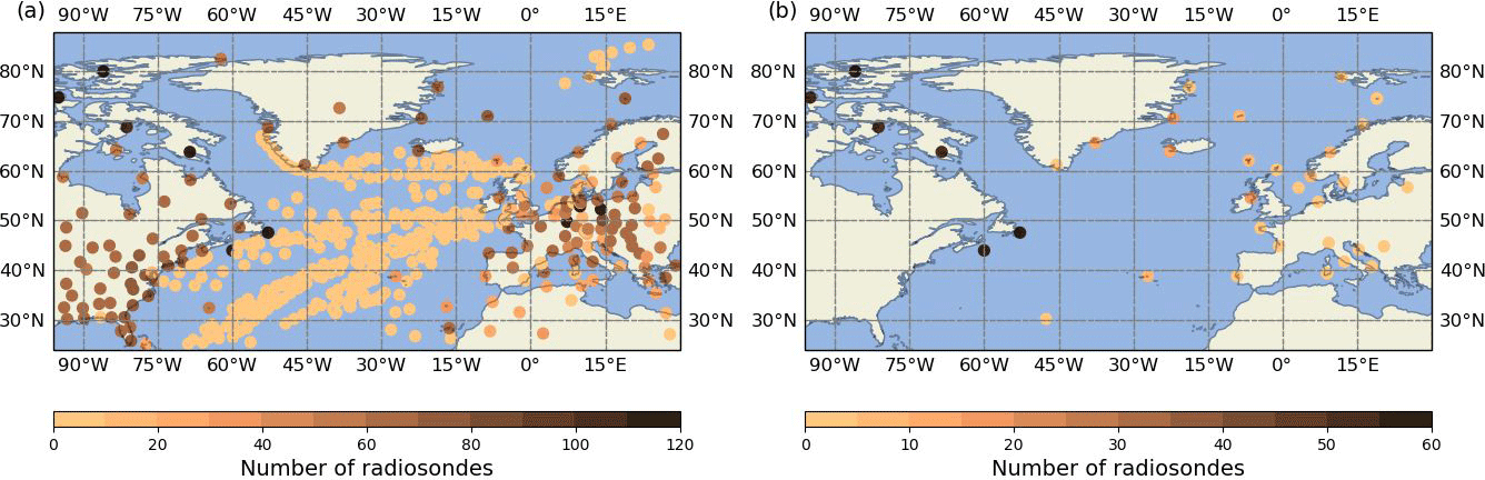
Figure 1 Positions of radiosonde launches that were assimilated by the ECMWF IFS between 17 September and 18 October 2016 for (a) all radiosondes (9729) and (b) the subset of 497 non-operational radiosondes launched during NAWDEX. The coloring denotes the number of assimilated profiles at a particular site. The scale of the color bar changes between (a) and (b).

To investigate the influence of the extra radiosonde observations during NAWDEX, a dedicated OSE was performed with the IFS (Schindler et al., 2020). The cycled OSE covers the whole NAWDEX campaign period (17 September to 18 October) and uses IFS model cycle 43r1 (Cy43r1; ECMWF, 2016), which became operational in November 2016. The triangular–cubic–octahedral grid (TCo1279​​​​​​​​​​​​​​​​​​​​​) provides a horizontal resolution of ∼ 9 km and 137 vertical sigma-hybrid levels that range from the surface up to ∼ 80 km. The vertical resolution is highest in the planetary boundary layer and decreases with altitude. At typical midlatitude tropopause altitudes (6–15 km; e.g., Schäfler et al., 2020) the vertical grid spacing is about 300 m. The incremental hybrid 4DVAR DA scheme used at ECMWF assimilates observations available in a 12 h time window to update a prior short-range forecast in order to achieve the best possible estimation of the atmospheric state, which is the analysis. (More details about the implementation of 4DVAR in the IFS are given in Rabier et al., 2000, or in the IFS documentation ECWMF, 2016.) As in the operational ECMWF system, the B matrix for the experiments is based on a blended combination of a climatological estimate and an estimate from an ensemble of data assimilations (EDA). The cycled OSE comprises two separate model runs. The control run (CTR) considered all routine and extra radiosondes as well as the dropsondes launched during NAWDEX. The denial (DEN) run excluded all additional observations in a region over the North Atlantic (25–90° N; 82° W–30° E). In addition, a 25-member EDA experiment was conducted at lower horizontal resolution (TCo639 ∼ 18 km) for both experiments. (More details on the OSE design are given in Schindler et al., 2020.)

For our analysis we retrieved observation feedback files of the OSE experiment from ECMWF's observation database (ODB), which contain the (radiosonde) temperature and wind observations as well as their departures from the background and analysis state given as profiles using pressure as the vertical coordinate. On the one hand, we analyze the influence of all 9729 radiosondes in the operational CTR run, and on the other, the influence of the subset of 497 radiosondes in the CRL is compared with the DEN experiment, where they were excluded and only passively monitored. The observation space data are stored during the 4DVAR process at the position and time of the observations. It has to be noted that the radiosonde profiles are not assimilated at their fully measured vertical resolution (which would be ∼ 5 m) but at a reduced number of levels (∼ 50–350), which depends on the reporting type (alphanumeric, BUFR, etc.) the individual stations used for the data transmission to the Global Telecommunications System (GTS) (Ingleby et al., 2016). About 65 % of the assimilated radiosonde profiles used in this study have a low vertical resolution (< 100 data points per profile), while 35 % of the profiles exhibit up to roughly 400 levels (see Fig. S1a in the Supplement). Accordingly, the distribution of the average vertical distance of neighboring data points in the UTLS shows a bi-modal shape and varies between ∼ 100 and 400 m in the UTLS (Fig. S1b). Cy43r1 does not consider the horizontal drift of the radiosondes. From the requested feedback files, we extract those observations that are actively assimilated. Some profiles (< 1 %) which do not provide temperature and wind data above the 540 hPa level (∼ 5 km) are excluded from the statistical analysis. This level is selected as it serves as a starting point for tropopause detection (Sect. 2.2).

2.2 Data processing and tropopause-relative coordinates

First, the observation space background (or first guess; y_FG) and analysis (y_AN) states are derived from the observations (y_O) and departures from the first guess (dep_FG; referred to as innovation) and the analysis (dep_AN; hereafter referred to as residual) as follows:

$$\begin{array}{}\text{(1)}& {\displaystyle }\text{innovation:}{\text{dep}}_{\text{FG}}=y_{\text{O}}-y_{\text{FG}};\text{(2)}& {\displaystyle }\text{residual:}{\text{dep}}_{\text{AN}}=y_{\text{O}}-y_{\text{AN}}.\end{array}$$

The observation space increment is defined as the analysis minus the background state and shows whether a quantity has been increased or decreased in the DA cycle:

$$\begin{array}{}\text{(3)}& \text{Increment}=y_{\text{AN}}-y_{\text{FG}}.\end{array}$$

In the next step, we derive the geometrical altitude from the pressure data based on the hydrostatic equation as described in ECMWF (2016). The observation and model states are then linearly interpolated onto a vertical equidistant 10 m grid. The potential temperature (θ) and the squared static stability (N²) are computed from the temperature profile using

$$\begin{array}{}\text{(4)}& N^{\mathrm{2}}=\left(-{\displaystyle \frac{g}{\mathit{\theta }}}\right)\times \left(-{\displaystyle \frac{\text{d}\mathit{\theta }}{\text{d}z}}\right)\left[{\displaystyle \frac{\mathrm{1}}{s^{\mathrm{2}}}}\right],\end{array}$$

with $\frac{\text{d}\mathit{\theta }}{\text{d}z}$ being the vertical gradient of θ in geometrical coordinates (z) and g the gravitational acceleration (g = 9.81 m s⁻²).

From the wind profile, the vertical wind shear of the horizontal wind speed (hereafter referred to as wind shear) is calculated as follows:

$$\begin{array}{}\text{(5)}& \text{wind shear}=\left({\displaystyle \frac{\text{d}\left|\mathit{u}\right|}{\text{d}z}}\right)\left[{\text{s}}^{-\mathrm{1}}\right],\end{array}$$

with $\frac{\text{d}\left|\mathit{u}\right|}{\text{d}z}$ being the vertical gradient of the magnitude of the horizontal wind vector u.

In the statistical assessment, the average profiles of the parameters and increments are calculated in tropopause-relative coordinates. Various tropopause definitions are used in the literature which are defined based on the particular thermal, dynamic, and chemical characteristics of the UTLS (e.g., Gettelman et al., 2011). We rely on the lapse–rate tropopause (LRT), which, by definition, points to the sharp transition of thermal stratification from the UT to the LS (e.g., Birner et al., 2002; Tinney et al., 2022). The LRT is defined as the lowest level at which the lapse rate (i.e., the vertical temperature gradient) falls below 2 K km⁻¹, subject to the condition that the average lapse rate from that level to any point within the overlying 2 km layer does not exceed 2 K km⁻¹. This World Meteorological Organization (WMO) definition (WMO, 1957) also comprises a further criterion to determine a secondary (or “double”) tropopause; however, in the presented analysis we determine only the “first” LRT. The LRT altitude is used to determine LRT-relative altitudes (z_LRT-relative) for each radiosonde profile, which is the difference of the geometrical height profile (z_geometrical) and the LRT altitude (z_LRT) following Eq. (6):

$$\begin{array}{}\text{(6)}& z_{\text{LRT-relative}}=z_{\text{geometrical}}-z_{\text{LRT}}.\end{array}$$

Although the LRT definition permits a robust detection of tropopause altitude for most atmospheric conditions, the 2 K criterion entails some important limitations (for details see Tinney et al., 2022, and references therein). First, the 2 K threshold can lead to undesired false detections of the LRT altitude (hereafter referred to as “misdetection”) at small temperature fluctuations which are often present in the lower troposphere (boundary layer) but also occur in the mid-troposphere. To avoid LRT misdetection, tropopause detection is performed above ∼ 5 km (540 hPa) altitude. Second, in situations of weak vertical temperature gradients, i.e., smooth transitions across the tropopause, the 2 K threshold is sometimes not quite met leading to LRT jumps by several kilometers for neighboring, similar temperature profiles (Krüger et al., 2022). This occurs typically in the vicinity of the jet streams where tropopause altitude shows a discontinuity or double tropopauses may occur (Pan et al., 2004; Hoffmann and Spang, 2022; Tinney et al., 2022). Hence, a slightly different temperature representation in models and observations can result in large LRT altitude differences. The potential influence of such misdetections is discussed in Sects. 3.2.2 and 4.

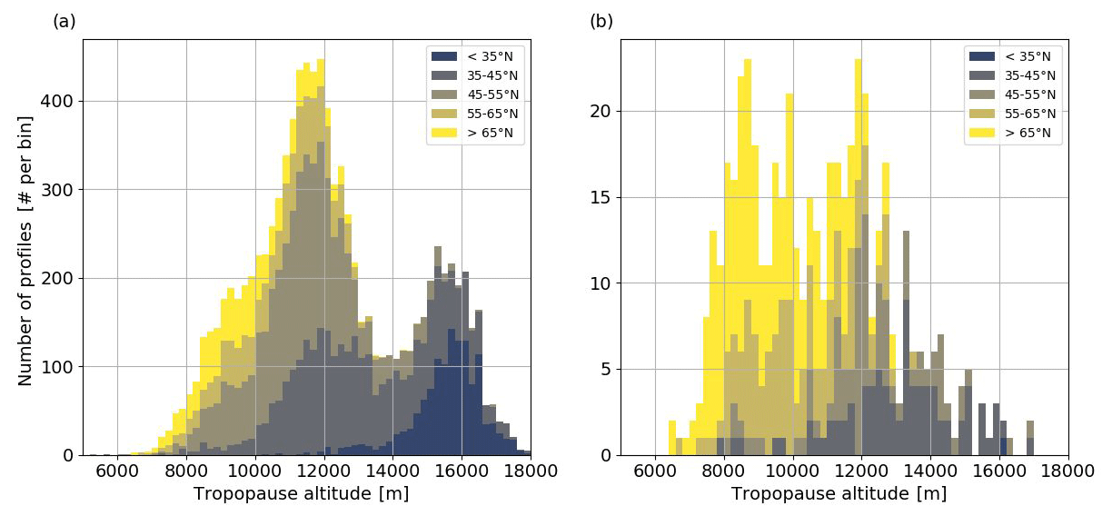
Figure 2 Stacked distribution of LRT${}_{y_{\text{O}}}$ with 0.2 km bin size for (a) all 9729 radiosondes and (b) the additional 497 radiosondes observed during NAWDEX. The coloring shows the latitudes of the radiosonde stations (10° bins).

LRT altitudes are derived individually for the observations (hereafter referred to as LRT${}_{y_{\text{O}}}$), the background (LRT${}_{y_{\text{FG}}}$), and the analysis (LRT${}_{y_{\text{AN}}}$) by following the WMO definition outlined above. Figure 2a illustrates the vertical distribution of LRT${}_{y_{\text{O}}}$ for 9729 profiles which has a bi-modal shape in the altitude range of 6–18 km with peaks at 11.5 and 15.5 km. The left mode represents profiles with a high frequency (75 % of the profiles) of LRT altitudes at 10–14 km (see Fig. 2a) which is typical for the midlatitudes in autumn (e.g., Hoffmann and Spang, 2022; Krüger et al., 2022). Its broad spectrum is related to the variability in the midlatitude tropopause altitude in different synoptic situations, e.g., in ridges and troughs (e.g., Hoerling et al., 1991). The right mode (LRT > 14 km; 25 % of the profiles) with its smaller maximum indicates profiles in the subtropics. The LRT distribution for the additional NAWDEX radiosondes (Fig. 2b) does not exhibit a corresponding second peak, due to the low number of soundings conducted at latitudes < 40° N.

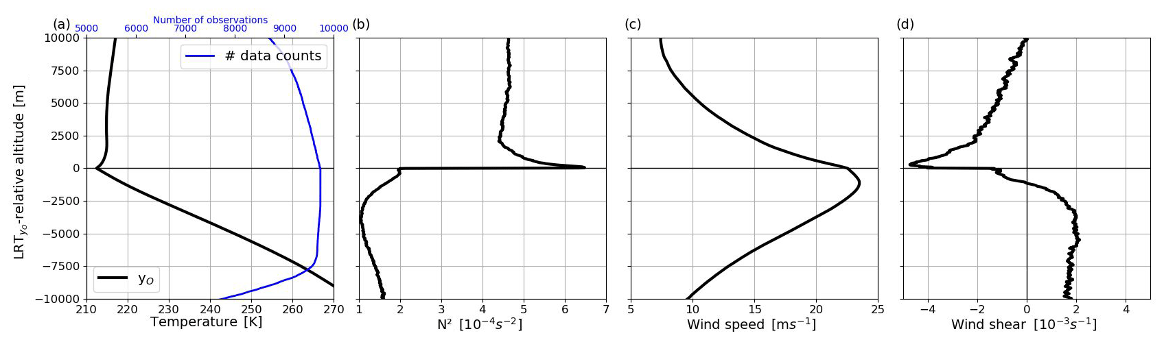
Figure 3 LRT${}_{y_{\text{O}}}$-relative mean profiles of, using 9729 radiosondes, (a) temperature (black line) and number of data (blue line), (b) N², (c) wind speed, and (d) wind shear.

Figure 3 presents the mean vertical profiles of observed temperature, N², wind speed, and wind shear profiles averaged in LRT${}_{y_{\text{O}}}$-relative (with respect to the observed tropopause) coordinates. These profiles outline the main characteristics of the midlatitude tropopause that are known from climatology (e.g., Birner et al., 2002; Grise et al., 2010; Hoffmann and Spang, 2022): above a linearly decreasing temperature in the troposphere (∼ 7 K km⁻¹), a temperature minimum of about 213 K is reached at LRT${}_{y_{\text{O}}}$. Above the tropopause, a distinct temperature inversion (0–1.5 km above LRT${}_{y_{\text{O}}}$) is observed, followed by an isothermal temperature profile in the stratosphere (up to ∼ 5 km above the LRT${}_{y_{\text{O}}}$). This change in stratification results in a rapid jump in N² (from 2 to 6.5 × 10⁻⁴ s⁻²) across the LRT${}_{y_{\text{O}}}$ altitude. Wind speed continuously increases with altitude in the troposphere up to a maximum (∼ 23.5 m s⁻¹) at ∼ 1 km below LRT${}_{y_{\text{O}}}$. Corresponding to the distribution of wind speed, the vertical shear of wind speed is positive up to the wind speed maximum, then abruptly decreases beyond and reaches a distinct minimum (∼ 5 × 10⁻³ s⁻¹) at about 300 m above LRT${}_{y_{\text{O}}}$. Note that the presented data set of 9729 radiosondes provides a high data coverage (blue line in Fig. 3a) in the UTLS.

A separate analysis of extratropical (LRT < 14 km) and subtropical (LRT > 14 km) observations reveals similar shapes for the extratropical and the overall data (see Fig. S2a, b, c, d). The subtropical mean profiles exhibit lower temperatures in the entire UTLS, a weaker temperature inversion in the LS, and no wind maximum located near the tropopause.

3 Results

3.1 Increments in geometrical and tropopause-relative coordinates

Figure 4 shows the time series of temperature increments over Iqaluit, Canada, between 17 September and 18 October 2016, in both geometrical (Fig. 4a) and LRT${}_{y_{\text{O}}}$-relative (Fig. 4b) coordinates. Iqaluit is selected as it comprises a high number of radiosonde profiles (114 profiles at 6-hourly intervals) and outlines the typical high tropopause altitude and wind speed variability related to the changing synoptic situations. Several strong jet stream events with wind speeds of occasionally > 45 m s⁻¹ passed over the station, which are accompanied by high variability in the LRT (7–13 km).

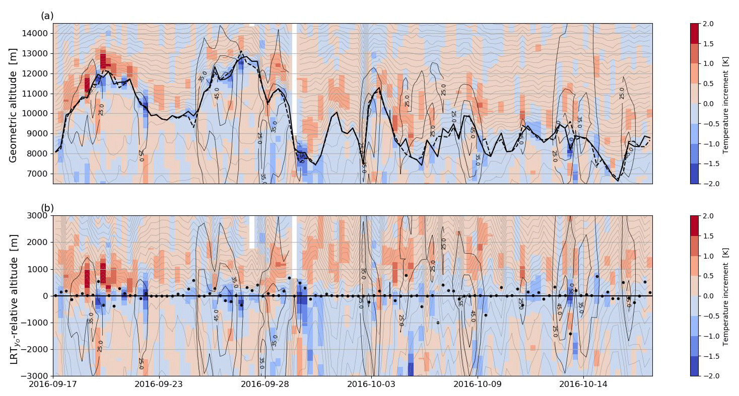
Figure 4 Time series (17 September to 18 October 2016) of temperature increments (color shading) at Iqaluit (63.75° N, 68.53° W), Canada, illustrated in (a) geometrical height and (b) LRT${}_{y_{\text{O}}}$-relative coordinates. The panels are superimposed by the observed θ (thin gray lines; Δθ=4 K) and wind speed (thin black contours). In (a) the solid (dashed) black line shows LRT${}_{y_{\text{O}}}$ (LRT${}_{y_{\text{FG}}}$). The black dots in (b) show the difference of LRT${}_{y_{\text{O}}}$ and LRT${}_{y_{\text{FG}}}$.

In geometrical altitude strong positive (> 1 K) and negative temperature increments (< −1 K) are stacked and roughly follow the tropopause. Due to the variable LRT altitude, averaging of the profiles in geometrical coordinates would blur the vertical distribution of the increments and thus hide a potential influence on the tropopause in a statistical evaluation. However, in LRT${}_{y_{\text{O}}}$-relative coordinates, the negative increments can be clearly assigned to a layer of about ±0.5 km around the tropopause and the positive increments to the 2 km-thick layer above it. The vertical extent of the positive and negative increments is relatively persistent along the entire time series, but the magnitude is variable. The distance between observed and background tropopause altitude is mostly in the range of ∼ 100 m, but there are also cases with large altitude differences (> 1 km; see discussion in Sect. 2.3).

3.2 Statistical assessment

3.2.1 Mean tropopause-relative influence

Figure 5 presents LRT${}_{y_{\text{O}}}$-relative average profiles of temperature, N², wind speed, and vertical wind shear for the 9729 radiosondes and their model equivalents. The minimum temperature detected in a layer of ±500 m around LRT${}_{y_{\text{O}}}$ is overestimated (by up to 1 K) in the background profiles (Fig. 5a) confirming a warm temperature bias at the tropopause. In the LS above, the background temperature increases less strongly which results in a cold model bias between 0.5 and 2 km above the tropopause. The weaker thermal gradients in the background are accompanied by an underrepresentation of the amplitude and sharpness of the N² jump across the tropopause (Fig. 5b). Wind speed is underestimated in the background throughout the UTLS (Fig. 5c), with a maximum underestimation (0.5 m s⁻¹) between −1 and 0.5 km. The rapid decrease in wind shear above the wind maximum towards the lowermost 1 km layer of the LS is less pronounced in the background. Figure 5a–d show that the analysis is drawn towards the observations for all parameters at any altitude in the UTLS. The slightly sharper tropopause structure reveals a positive influence of DA on the representation of the tropopause in the analysis.

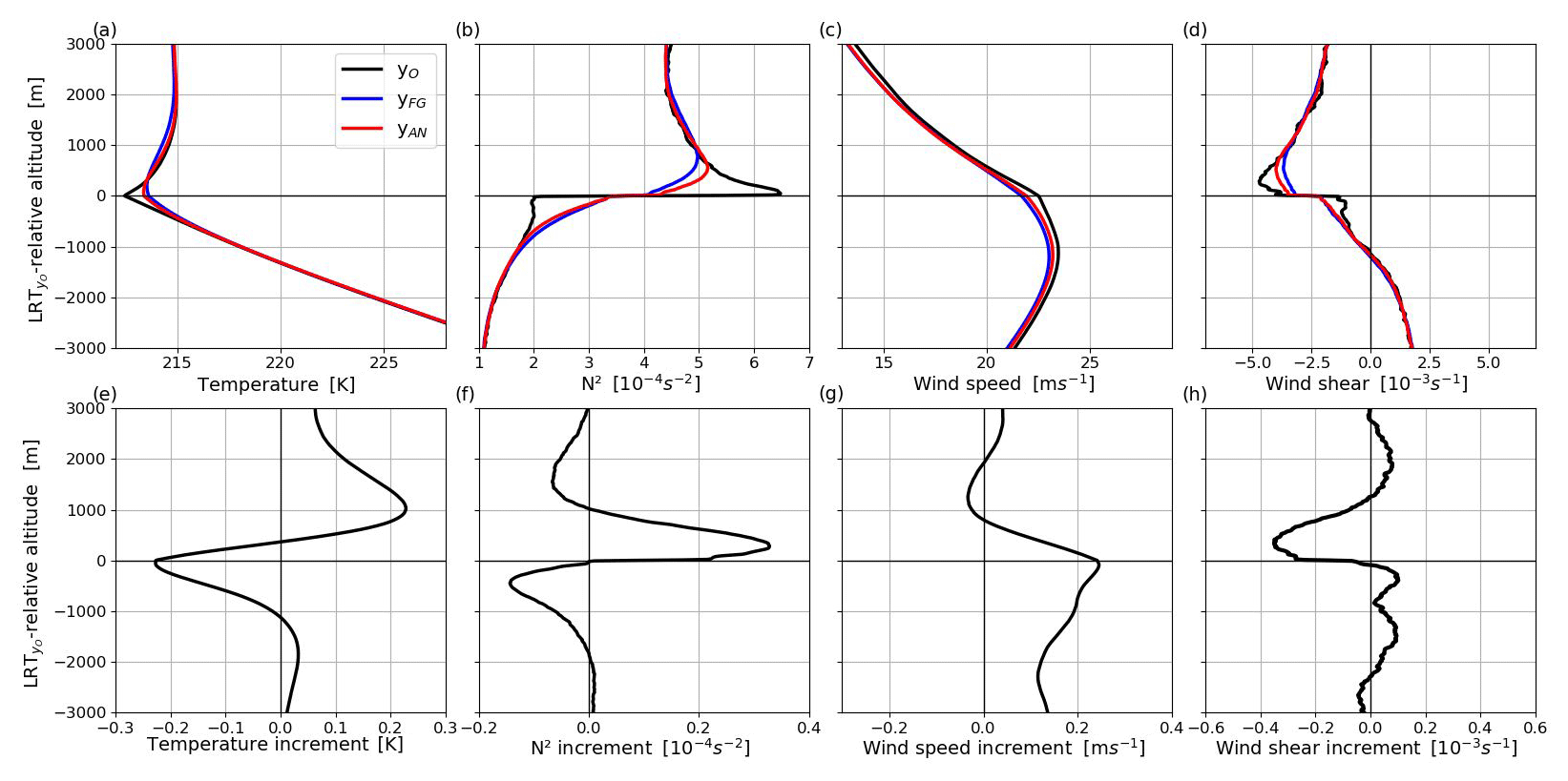
Figure 5 LRT${}_{y_{\text{O}}}$-relative distributions of (a) temperature, (b) N², (c) wind speed, and (d) wind shear, as well as the respective increments ((e–h); Eq. 3), averaged for the 9729 profiles of observations (black line), background (blue line), and analysis (red line).

Figure 5e–h show the vertical structure of the increments. The temperature increments (Fig. 5d) imply a cooling (up to −0.25 K) between −1 and +0.5 km around LRT${}_{y_{\text{O}}}$, i.e., the altitude range of the warm bias. In the LS, a warming of up to 0.25 K between 0.5 and 2 km above LRT${}_{y_{\text{O}}}$ counteracts the cold bias in the model background. This impact on the temperature distribution results in negative N² increments (−0.15 × 10⁻⁴ s⁻²) in a 1.5 km-thick layer below LRT${}_{y_{\text{O}}}$ and between 1 and 2 km above LRT${}_{y_{\text{O}}}$ (Fig. 5e). In the 1 km layer above LRT${}_{y_{\text{O}}}$, N² increments are positive with a distinct maximum of ∼ 0.32 × 10⁻⁴ s⁻² at ∼ 0.5 km. Wind increments are predominantly positive in the entire UTLS (Fig. 5g), which indicates a wind speed increase in the analysis. The wind increments are stronger in the UT than in the LS peaking (0.25 m s⁻¹) at the altitude of the wind maximum and the strongest underestimation in the background (the 1 km layer below LRT${}_{y_{\text{O}}}$; Fig. 5c). Increments in wind shear are positive in the 2 km below, and negative in the 1 km layer above, LRT${}_{y_{\text{O}}}$ (minimum at ∼ 500 m above LRT${}_{y_{\text{O}}}$). Between ∼ 1.5 and 3 km above LRT${}_{y_{\text{O}}}$, wind shear increments are positive and of comparable magnitude to the UT. A separate analysis of midlatitude and subtropical increments (Fig. S3) shows that the latter are weaker. However, as the increments in both regions point in the same direction, the complete data are considered for the statistical analysis in the remainder of this article.

3.2.2 Sensitivity to the LRT-relative coordinate

Figure 5 presents profiles of the parameters and increments relative to the observed tropopause. However, from Fig. 4 we have seen that the observed tropopause altitude may differ from the background (and analysis). This raises the question of which LRT-relative view is the most suitable reference for evaluating tropopause structure. In the following, we present the distributions in different LRT-relative reference systems and discuss their significance to evaluate tropopause sharpness. Figure 6 illustrates the profiles of temperature and N² in the observations (Fig. 6a, e), background (Fig. 6b, f), and analysis (Fig. 6c, g) with respect to the observed LRT${}_{y_{\text{O}}}$, the background LRT${}_{y_{\text{FG}}}$, and the analysis LRT${}_{y_{\text{AN}}}$, respectively. In each case the lowest tropopause temperature as well as the strongest temperature inversion and jump in N² occurs when the “own” LRT is used. This is particularly obvious for the observed profile relative to LRT${}_{y_{\text{O}}}$ (black line in Fig. 6a, e). In addition, the background and analysis profiles have the lowest tropopause temperature and strongest inversion when viewed relative to LRT${}_{y_{\text{FG}}}$ (medium red line in Fig. 6b) and LRT${}_{y_{\text{AN}}}$ (light blue line in Fig. 6c), respectively. Figure 6d and h show the increments referenced to the different LRT-relative coordinates. Each of the LRT reference systems confirms a cooling near the LRT, a warming in the LS (Fig. 6d), and an increase in static stability just above the LRT (Fig. 6h). The differing LRT altitudes of the individual profiles in y_O, y_FG, and y_AN result in small differences in the magnitude of the increments for the different LRT-relative coordinates (discussed in further detail in Sect. 3.3). The increments are smallest when referenced to LRT${}_{y_{\text{FG}}}$.

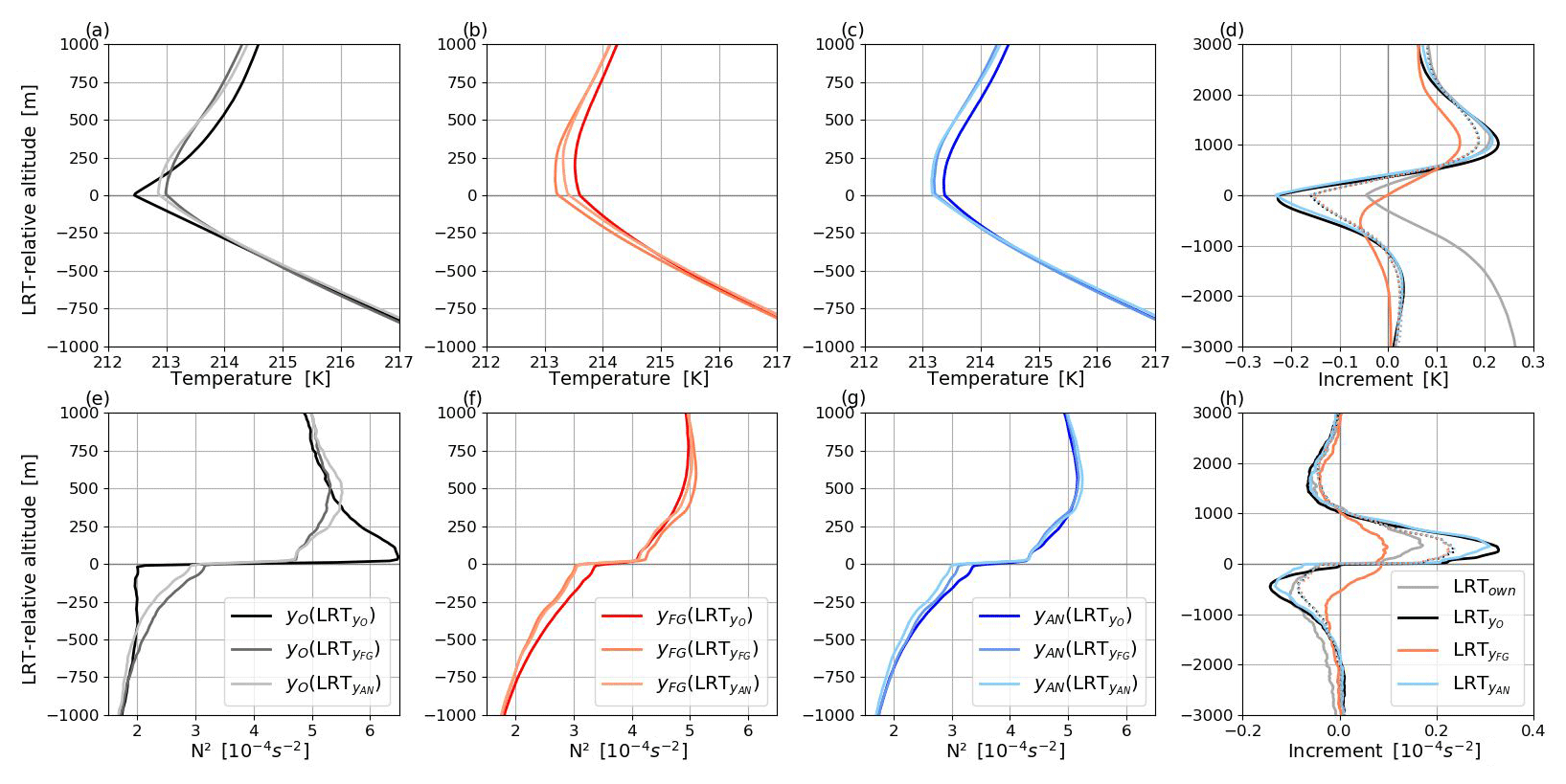
Figure 6 Mean profiles of temperature (a–c) and N² (e–g) for observations (a, e), background (b, f), and the analysis (c, g) relative to LRT${}_{y_{\text{O}}}$, LRT${}_{y_{\text{FG}}}$, and LRT${}_{y_{\text{AN}}}$, respectively (color coded). Panels (d) and (h) show the associated increments. In addition, increments using the own LRTs are shown (gray line, calculated as $y_{\text{AN}}\left({\text{LRT}}_{y_{\text{AN}}}\right)-y_{\text{FG}}\left({\text{LRT}}_{y_{\text{FG}}}\right)$; for details see text). The dotted lines in (d) and (h) represent the 3712 profiles with the LRT altitudes of observations, background, and analysis being within ±100 m. (Note that the dotted lines overlap.)

As the LRT_own-relative distributions provide the highest sharpness, we also consider LRT_own-relative increments (gray line in Fig. 6d, h) to further analyze the influence on tropopause sharpness. These increments in LRT_own-relative coordinates, which are calculated as $y_{\text{AN}}\left({\text{LRT}}_{y_{\text{AN}}}\right)-y_{\text{FG}}\left({\text{LRT}}_{y_{\text{FG}}}\right)$ and ideally remove effects on the average increments from differing LRT${}_{y_{\text{FG}}}$ and LRT${}_{y_{\text{AN}}}$ altitudes, have a comparable structure in the LS. However, they show only a slight cooling (< 0.1 K) at the tropopause and an increasing warming with decreasing altitude in the troposphere, which does not agree with increments in geometrical and LRT${}_{y_{\text{O}}}$ space (e.g., Figs. 4, 6a). The warming in the troposphere is a systematic temperature bias that is caused by the tropopauses detected at different altitudes (either in LRT${}_{y_{\text{FG}}}$ or in LRT${}_{y_{\text{AN}}}$, or both; Fig. 6a). To emphasize the role of differing tropopause altitudes on the distribution of the increments, the four types of increments are shown for cases with similar LRT altitudes (within ±100 m), which are almost identical (see overlapping dotted lines in Fig. 6d). We do not further pursue the analysis of LRT_own-relative increments because such increments are determined after shifting the profiles with respect to the own LRT which does not correspond to real changes to the model background field in geometrical space (when the LRT${}_{y_{\text{FG}}}$ and LRT${}_{y_{\text{AN}}}$ differ). We nonetheless present this analysis to emphasize the sensitivity of cross-tropopause distributions and their increments to the choice of the LRT reference and the impact of systematic LRT altitude differences. LRT${}_{y_{\text{O}}}$ provides the most realistic representation of tropopause altitude (Figs. 4a, 6a) and is used in the following to analyze the influence on tropopause sharpness in this study. In addition, the influence on tropopause altitude is studied relative to the LRT${}_{y_{\text{FG}}}$ (Sect. 3.3).

3.2.3 Influence on tropopause sharpness

The previous results indicated an increase in tropopause sharpness in the analysis with suggested high temporal variability in the increments (Fig. 4) that is likely influenced by particular dynamical situations. Figure 7a illustrates the distribution of the observed maximum squared static stability ($N_{max}^{\mathrm{2}}$) in the 3 km above LRT${}_{y_{\text{O}}}$, which is a common indicator for tropopause sharpness (Birner et al., 2006; Pilch Kedziersky et al., 2015). $N_{max}^{\mathrm{2}}$ shows a uni-modal, positively skewed distribution ranging from 3 to 30 × 10⁻⁴ s⁻² with the largest frequency (> 200 profiles per bin) of between 6–12 × 10⁻⁴ s⁻² and the lowest frequency (< 50 profiles per bin) for 5 × 10⁻⁴ s⁻² < $N_{max}^{\mathrm{2}}$ and $N_{max}^{\mathrm{2}}$ > 15 × 10⁻⁴ s⁻². The quartiles of this distribution are used to classify the data into the smoothest $\left(N_{max,Q\mathrm{00}\text{–}Q\mathrm{25}}^{\mathrm{2}}\right)$, the intermediate $\left(N_{max,Q\mathrm{25}\text{–}Q\mathrm{75}}^{\mathrm{2}}\right)$, and the sharpest $\left(N_{max,Q\mathrm{75}\text{–}Q\mathrm{100}}^{\mathrm{2}}\right)$ tropopause cases. The observed profiles (Fig. 7b) display that the sharp class has the lowest tropopause temperature and the strongest inversion with the largest jump in N². In contrast, the smoothest tropopauses exhibit a higher tropopause temperature, a weaker temperature inversion, and a lower amplitude in N² at LRT${}_{y_{\text{O}}}$. The intermediate class depicts a tropopause structure comparable to that of the full data set average described in Sect. 3.2.1. In agreement with these findings the observed mean tropopause altitude for the sharp and smooth classes are 12 750 and 11 580 m, respectively, which suggests that the sharp (smooth) tropopauses can be related to ridge (trough) situations characterized by high (low) tropopause altitudes. For the different $N_{max}^{\mathrm{2}}$ classes in Fig. 7, the wind profiles look similar (see Fig. S4), which is not surprising as high wind speeds in the jet are more related to the isentropic PV gradients (e.g., Bukenberger et al., 2023).

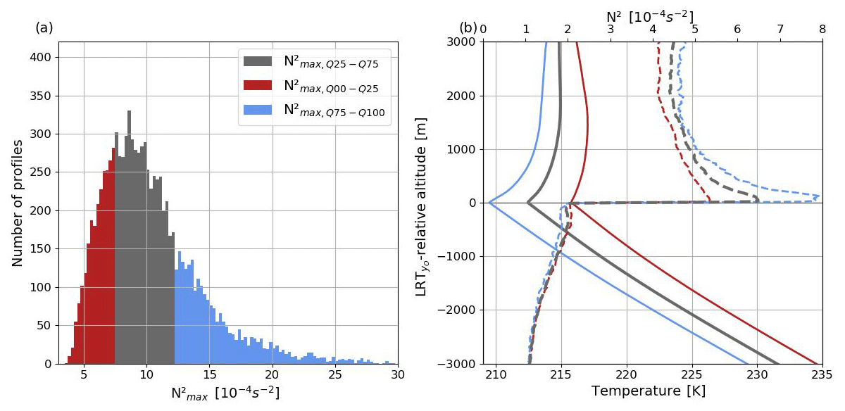
Figure 7 Panel (a) shows the distribution of $N_{max}^{\mathrm{2}}$ as observed in the 3 km layer above LRT${}_{y_{\text{O}}}$ with bin size 0.5 × 10⁻⁴ s⁻². Quartiles of the $N_{max}^{\mathrm{2}}$ distribution in (a) are used to classify tropopause sharpness: smoothest (red shading; Q00–Q25), intermediate (gray shading; Q25–Q75), and strongest sharpness (blue shading; Q75–Q100). Panel (b) shows the corresponding LRT${}_{y_{\text{O}}}$-relative mean profiles of observed temperature (solid lines) and N² (dashed lines).

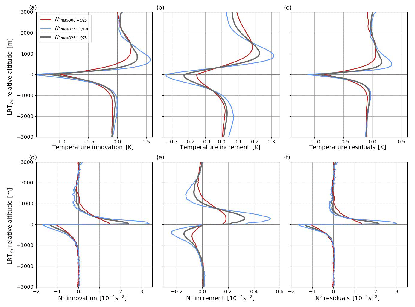
Figure 8 LRT${}_{y_{\text{O}}}$-relative mean profiles of innovations, increments, and residuals for (a–c) temperature and (d–f) N² for the classes of $N_{max}^{\mathrm{2}}$ defined in Fig. 7.

For each class of $N_{max}^{\mathrm{2}}$, the mean vertical profiles of innovation (Eq. 1), increment (Eq. 3), and residual (Eq. 2) for temperature and N² relative to LRT${}_{y_{\text{O}}}$ are presented in Fig. 8. We first focus on intermediate tropopause sharpness. In the UT, the temperature innovations are weak, negative, and vertically nearly constant (about−0.1 K; Fig. 8a) before they reach a minimum of about −1.2 K at LRT${}_{y_{\text{O}}}$ indicating a warm bias at the background tropopause. Above the tropopause, the innovations strongly increase and become positive at ∼ 0.5 km above LRT${}_{y_{\text{O}}}$ before a maximum cold bias of ∼ 0.3 K is reached at 0.8 km altitude. The temperature increments (Fig. 8b) correspond to the findings in Fig. 5, with the negative increments around LRT${}_{y_{\text{O}}}$ counteracting the warm bias and the positive increments above it decreasing the cold bias. In the ±0.5 km around LRT${}_{y_{\text{O}}}$ large N² innovations between −2 and 3 × 10⁻⁴ s⁻² illustrate the strong underestimation of tropopause sharpness in the background (Fig. 8d). The average positive (above LRT${}_{y_{\text{O}}}$) and negative (below LRT${}_{y_{\text{O}}}$) N² increments (Fig. 8e) for the intermediate profiles agree in shape and magnitude with the structure of N² increments given in Fig. 5. Apparently, they lead to sharpening of the tropopause. Increments are much smaller than the innovations (∼ 20 % for temperature and 10 % for N²) which explains why the vertical structure of the innovation is preserved in the residuals (Fig. 8c, f). For the smooth and sharp classes (blue and red lines in Fig. 8), innovations, increments, and residuals have a similar vertical distribution but show weaker and stronger amplitudes respectively. For instance, temperature increments are about −0.3 K (−0.1 K) at the tropopause for the sharp (smooth) class and about 0.3 K (0.1 K) for the maximum above, in the LS. The influence is stronger where the background biases are strongest.

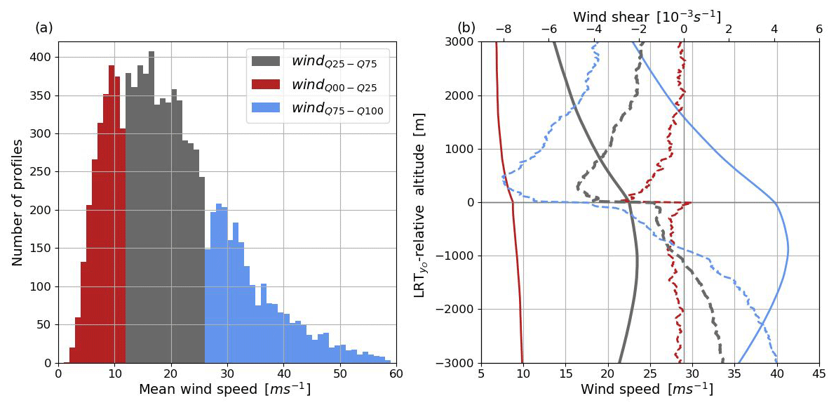
Figure 9 Panel (a) shows the distribution of mean observed wind speed in the ±3 km above and below LRT${}_{y_{\text{O}}}$ with 1 m s⁻¹ bin size. Quartiles of the distribution in (a) are used to distinguish wind classes: weakest wind (red shading; Q00–Q25), intermediate wind (gray shading; Q25–Q75), and strongest wind (blue shading; Q75–Q100). Panel (b) shows the corresponding LRT${}_{y_{\text{O}}}$-relative mean profiles of observed wind speed (solid lines) and wind shear (dashed lines) per class.

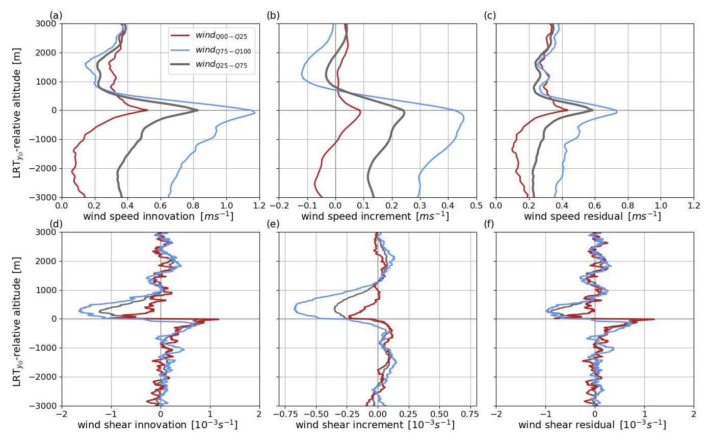
Figure 10 LRT${}_{y_{\text{O}}}$-relative mean profiles of wind speed and wind shear (a, d) innovations, (b, e) increments and (c, f) residuals per classes as defined in Fig. 9.

Figure 9 illustrates the variability in wind speed in the radiosonde data set. Average wind speeds in a layer of ±3 km around LRT${}_{y_{\text{O}}}$ range from nearly 0 to 60 m s⁻¹ with the highest frequency between 5 and 25 m s⁻¹ (Fig. 9a). Quartiles of layer-mean wind speed divide the data set into weak (wind_Q00–Q25), intermediate (wind_Q25–Q75), and strong (wind_Q75–Q100) winds. The weak wind class shows vertically fairly constant low wind speeds (< 10 m s⁻¹). While the intermediate class exhibits a shape of the mean wind profile comparable to that of the full data set (Fig. 5), the strong wind class depicts a pronounced wind maximum (> 40 m s⁻¹) at −1 km altitude below LRT${}_{y_{\text{O}}}$ expressing strong jet stream winds. While wind shear in the weak wind class is small, the intermediate and strong wind classes have a decrease in vertical wind shear from positive values below the wind maximum to negative values above it, with a peak in the LS. All classes show an increased reduction in wind speed above the LRT which is associated with a step change in vertical wind shear. The mean profiles of innovation, increment, and residual for each class are shown in Fig. 10. The positive wind innovations of all classes across the UTLS express the underestimated wind speeds in the background (Fig. 10a; see also Fig. 5). Innovations in the UT are generally larger than in the LS and peak at the tropopause. Maximum innovations range between 0.5 m s⁻¹ for the weak wind class and 1.2 m s⁻¹ for the strong wind class. The predominately positive wind speed increments throughout the UTLS (Fig. 10b) represent a wind increase in the analysis which is largest in the 500 m layer below LRT${}_{y_{\text{O}}}$, ranging between 0.1 m s⁻¹ for the weak wind class and 0.45 m s⁻¹ for the strong wind class. The positive wind speed residuals (Fig. 10c) show that a slow wind bias remains in the analysis; however, the weaker residuals than the innovations observed for each class point to an improvement. For the strongest winds the innovations are reduced by roughly 40 %. In the layer with increased negative shear directly above the LRT, there are particularly strong negative shear innovations for the class of the strong winds, which are associated with increased negative shear increments. After the assimilation, wind shear residuals show little variability across all classes.

3.3 Influence on tropopause altitude

In the following, we investigate how modification of the temperature profile (Fig. 5e) affects tropopause altitude. Hereafter, LRT altitude differences between the observations and the background (${\text{LRT}}_{y_{\text{O}}}-{\text{LRT}}_{y_{\text{FG}}}$) are referred to as “LRT innovations” according to Eq. (1), and LRT altitude differences between the observations and the analyses are referred to as “LRT residuals” (${\text{LRT}}_{y_{\text{O}}}-{\text{LRT}}_{y_{\text{AN}}}$; Eq. 2). An overview of LRT innovations for the entire data set is given in Fig. 11a providing a symmetric, normal distribution centered near zero (−26 m). For 43 % of the profiles, the LRT innovations are in the range of ±100 m. For about 10 % of the profiles, LRT differences are larger than 1 km. In order to prevent an impact of misdetected LRTs (see discussion in Sect. 3.2.2), which are most likely for unusually large LRT differences, the following evaluation is restricted to 8778 profiles (∼ 90 %) which provide LRT altitude innovations within ±1 km.

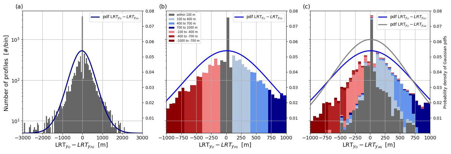
Figure 11 Distribution of (a) LRT innovations in the full data set, (b) as in (a) but for the range ±1000 m, and (c) LRT residuals. The color coding reflects intervals of LRT innovations shown in (b) and is reused in (c) to visualize the LRT altitude change in LRT${}_{y_{\text{AN}}}$ (for details see text). Gaussian probability density functions (pdf) are given in lines of dark blue, blue, and gray, respectively, for 50 m bins. Note the log scale of the y axis.

First, we compare the LRT innovations (Fig. 11b, subset of Fig. 11a) and LRT residuals (Fig. 11c), which are color coded at different intervals of LRT innovations. The gray interval reflects LRT innovations within ±100 m, while bluish colors represent profiles where the observed LRT is higher than the background, and vice versa for reddish colors. Comparing the color distributions in Fig. 11b and c allows interval changes to be identified, and only a small fraction of profiles change the intervals. The distribution of LRT innovations shows a clear maximum near zero with a frequency corresponding to about 3000 profiles per bin, and the frequency decreases towards the edges of the distribution to ∼ 10 profiles per bin. The distribution of LRT residuals (Fig. 11c) shows a slightly increased number (+15 %) of profiles within ±100 m indicating an improved tropopause altitude in the analysis and this improvement is confirmed by a slightly narrower shape of the Gaussian fit of the LRT residuals compared with the LRT innovations.

Table 1 Number of profiles, averaged observed LRT altitude, innovation, residual, and improvement for different intervals of LRT innovation (see Fig. 11b). The improvement is defined as the averaged $|{\text{LRT}}_{y_{\text{O}}}-{\text{LRT}}_{y_{\text{FG}}}|-|{\text{LRT}}_{y_{\text{O}}}-{\text{LRT}}_{y_{\text{AN}}}|$, so positive values reflect improved LRT altitude in the analysis.

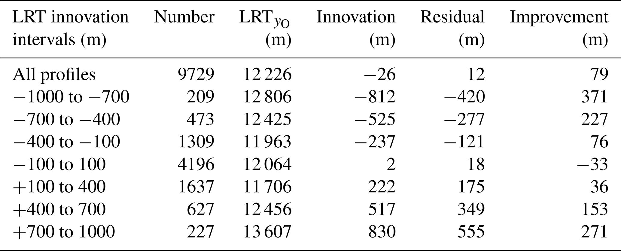
For the different intervals of LRT innovations in Fig. 11, Table 1 provides the number of profiles, the mean LRT${}_{y_{\text{O}}}$ altitude, as well as the mean innovation, residual, and improvement. Except for the interval with the smallest innovation (±100 m; gray interval), the average innovation is larger than the residual which implies a vertical shift in LRT${}_{y_{\text{FG}}}$ towards LRT${}_{y_{\text{O}}}$. The generally positive influence is supported by the depicted improvements, defined as the absolute difference of innovation and residual. Interestingly, the LRT altitude shift and also the improvement grow with increasing distance between LRT${}_{y_{\text{O}}}$ and LRT${}_{y_{\text{FG}}}$.

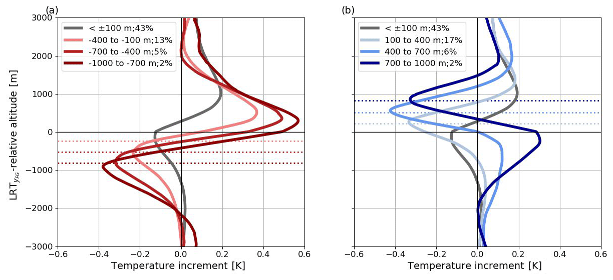
Figure 12 Mean temperature increments with respect to LRT${}_{y_{\text{FG}}}$-relative altitude for intervals of LRT innovations (color coding, following Fig. 11). Panel (a) shows negative LRT innovations (LRT${}_{y_{\text{O}}}$ < LRT${}_{y_{\text{FG}}}$; in red) and (b) positive LRT innovations (LRT${}_{y_{\text{O}}}$ > LRT${}_{y_{\text{FG}}}$; in blue). The gray lines show the increment for LRT innovations within ±100 m. In (a) and (b) the averaged LRT${}_{y_{\text{FG}}}$-relative altitude of LRT${}_{y_{\text{O}}}$ for each interval is depicted by the dotted lines.

In order to understand how the LRT altitude changes are related to the changes in the background temperature profile, the average temperature increments for the individual intervals of LRT innovations are presented with respect to the LRT${}_{y_{\text{FG}}}$-relative altitude (Fig. 12). For small LRT innovations (within ±100 m; gray line in Fig. 12a, b), the temperature increments are negative at the LRT (−0.15 K) and positive in the LS (0.2 K) (analogous to the sharpening influence discussed in Sects. 3.1 and 3.2) which does not lead to major changes in LRT altitude in this interval (see Table 1). With increasing LRT innovations, the altitudes of the peaks in the LRT${}_{y_{\text{FG}}}$-relative increments are vertically shifted. In cases of negative LRT innovations (Fig. 12a), which means that the observed LRT${}_{y_{\text{O}}}$ is located lower than the background LRT${}_{y_{\text{FG}}}$, we observe positive increments (warming, 0.3–0.6 K) at and above LRT${}_{y_{\text{FG}}}$ as well as negative increments (cooling, 0.2–0.4 K) below LRT${}_{y_{\text{FG}}}$. As the strongest negative increments agree with the observed tropopause altitude (dotted lines in Fig. 12a), peaks in the increments are shifted downwards and show slightly higher maxima for increasing negative LRT innovations (red profiles in Fig. 12a). In contrast, positive LRT innovations (i.e., LRT${}_{y_{\text{O}}}$ located above LRT${}_{y_{\text{FG}}}$; Fig. 12b) exhibit negative increments (−0.3 to −0.4 K) above LRT${}_{y_{\text{FG}}}$ and positive increments below LRT${}_{y_{\text{FG}}}$. Here, the increment peaks are shifted upwards for more positive LRT innovations (blue profiles in Fig. 12b) in agreement with the altitude of the observed tropopause.

3.4 Attributing the influence to the radiosondes

The presented results reveal that DA sharpens the tropopause at the location of the radiosondes which provides a strong indication that this influence is related to the information contained in the radiosondes. However, a potential contribution of other observations cannot be excluded. For this reason, we compare the profiles and increments in the 497 NAWDEX radiosondes in the CTR run with the DEN run, in which they are denied and only passively monitored. The average profiles of observed temperature and N² of the 497 NAWDEX profiles (Fig. 13) are comparable to the average profiles of the 9729 radiosondes (Fig. 5) with a similar magnitude of the jump in N² and an alike decrease in wind shear across the tropopause. The average minimum temperature at the tropopause (Fig. 13a) is slightly higher (by ∼ 2 K) which is related to the observation locations of the NAWDEX radiosondes at higher latitudes (Fig. 2a, b) where the tropopause is typically lower and warmer. The additional radiosondes show a pronounced wind maximum below LRT${}_{y_{\text{O}}}$ of about 29 m s⁻¹ (Fig. 13c) which, compared with the lower wind speeds in the complete data set (Fig. 5c), indicates the occasionally strong jet streams in the focus of the NAWDEX campaign (Schäfler et al., 2018).

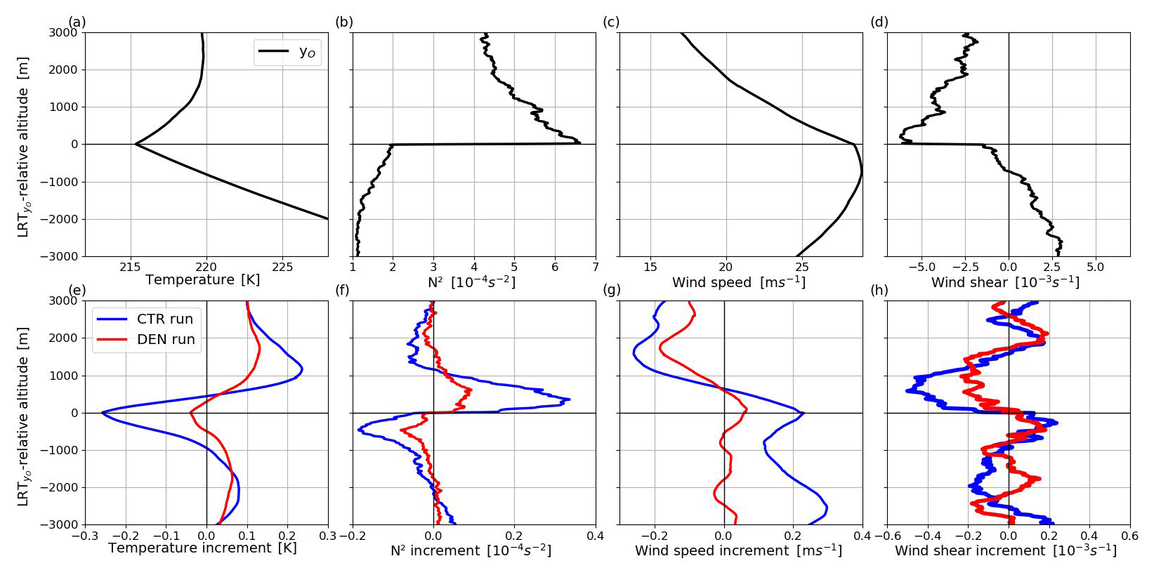
Figure 13 LRT${}_{y_{\text{O}}}$-relative mean profiles of the (a) temperature, (b) N², (c) wind speed, and (d) wind shear as observed by the 497 NAWDEX radiosondes and the respective increments in (e) temperature, (f) N², (g) wind speed, and (h) wind shear for the CTR (in blue) and DEN (in red) experiment.

The increments for temperature, N², wind speed, and wind shear for the subset of 497 additional NAWDEX radiosondes are presented in Fig. 13e and f. The CTR run exhibits a vertical structure that is comparable to that of the complete data set as discussed in Sect. 3.2: temperature increments are negative (−0.25 K) around the observed tropopause and positive in the LS (1–2 km above LRT${}_{y_{\text{O}}}$). Accordingly, the CTR N² increments possess a distribution similar to that of a 1 km layer of positive increments just above LRT${}_{y_{\text{O}}}$ with a maximum of 0.3 × 10⁻⁴ s⁻², weak negative increments (−0.2 × 10⁻⁴ s⁻²) in a 1 km layer beneath LRT${}_{y_{\text{O}}}$, and increments around ±0.1 × 10⁻⁴ s⁻² beyond the 1 km layers. The vertical structure of CTR wind speed increments for the NAWDEX radiosondes also agrees with the complete data set, with a positive increment (∼ 0.2 m s⁻¹) in the UT and a negative increment in the LS. Wind shear increments in the CTR run are also comparable to those of the full data set, but they show slightly lower values just above LRT${}_{y_{\text{O}}}$ (−0.5 × 10⁻³ s⁻¹) compared to the corresponding wind shear increments in Fig. 5h. The increments in temperature, N², wind speed, and wind shear in the DEN run (Fig. 13) are weaker at each altitude but tend to pick up a similar vertical distribution. This implies that the main contribution of tropopause sharpening and influence on wind comes from the assimilated radiosondes, but the non-zero DEN increments indicate that other observations also influence tropopause structure in the same direction. This may be due either to the remote impact of operational radiosondes or to dropsonde observations of which a larger number were deployed during NAWDEX (see Schindler et al., 2020). Further contributions of assimilated aircraft observations and GPS radio occultation data are also conceivable.

4 Discussion

In this study, we evaluate the influence of DA on the structure of the tropopause in the ECMWF IFS based on 9729 midlatitude radiosonde profiles. The statistical evaluation of observed temperature and wind, as well as derived N² and wind shear in (thermal) tropopause-relative coordinates, reproduces the typical sharp vertical gradients at the midlatitude tropopause (Birner et al., 2002). The LRT altitudes between 6 and 18 km during fall are considered to be representative for this area and season (e.g., Krüger et al., 2022).

To address the influence of DA on tropopause sharpness and altitude, the radiosonde and model states are transferred to tropopause-relative coordinates. The selection of a suitable reference is challenging because tropopause-relative distributions in observations, background, and analysis vary in the different LRT-relative coordinates due to slightly varying individual tropopause altitudes. Such LRT altitude differences may result from either misdetections caused by slight temperature fluctuations in the upper troposphere or from differences in the 3D temperature distribution, e.g., in the vicinity of the jet streams. Since the origin of these LRT altitude differences cannot clearly be identified and they affect the evaluation of the tropopause altitude's influence, we only consider LRT differences in the range of ±1 km. The sharpest tropopause in the observations, background, and analysis occur when viewed with respect to the “own” LRT. However, it turned out that the impact on sharpness cannot be assessed in own LRT coordinates as LRT altitude deviations in the background and analysis profiles cause a spurious tropospheric temperature bias. The observed tropopause as a reference provides the most accurate representation of the tropopause to evaluate the influence on tropopause sharpness. However, temperature increments with respect to the background tropopause are useful to better understand changes to the background profile. This shows that the tropopause reference system needs to be purposefully and carefully selected, and uncertainties related to tropopause detection need to be considered.

In this study, we highlight that DA improves the underestimated sharpness of the tropopause by introducing systematic changes to the background temperature and wind profile. The temperature innovations indicate a warm bias at the tropopause and a cold bias in the LS. In this layer of the sharp reversal in thermal stratification, N² is overestimated (underestimated) by the background below (above) the tropopause confirming findings by Birner et al. (2002). The temperature increments tend to move the background temperature towards the observations by decreasing the tropopause temperature by ∼ 0.25 K and increasing it with a similar magnitude in the LS above, which was already indicated by Radnóti et al. (2010) for the UTLS. The accompanied increase in N² (0.3 × 10⁻⁴ s⁻²) in a 1 km layer above the tropopause and a decrease in N² (∼ 0.2 × 10⁻⁴ s⁻²) in the uppermost troposphere is equivalent to tropopause sharpening, which is consistent in shape and magnitude with that of Pilch Kedziersky et al. (2016). Although the increments clearly reduce the background biases, the influence is rather small (∼ 10 %) compared with the innovations. The remaining LS cold bias in the analysis (0.2 K) corresponds to previous assessments (Radnóti et al., 2010) and is driven by radiative cooling due to water vapor (Sheperd et al., 2018; Bland et al., 2021), which is systematically overestimated at those levels (Krüger et al., 2022). Recent changes at the ECMWF reduced, but not fully removed, the bias in the IFS (Polichtchouk et al., 2021). The warm bias (1 K) at the tropopause in the IFS was related to the finite vertical resolution of the IFS incapable of fully resolving the tropopause (Ingleby et al., 2016), the assimilation of warm-biased aircraft data at tropopause flight levels (Ingleby, 2017), and the moist bias in the LS of the IFS (Bland et al., 2021). The magnitude of the warm bias (about 1.2 K) at the tropopause is about two to three times stronger than the corresponding warm bias reported in Bland et al. (2021). This difference may be related to vertical smoothing of the radiosonde profiles in Bland et al. (2021), which could lead to a higher tropopause temperature (König et al., 2019). Large N² biases (−2 to 3 × 10⁻⁴ s⁻²) in the analysis are found in the ±0.5 km layer around the tropopause. In addition, we show that the magnitude of tropopause sharpening depends on the dynamic situation. For sharper tropopauses, which are typically related to higher and thus colder tropopauses occurring in situations of upper-level ridges (Hoerling et al., 1991; Pilch Kedziersky et al., 2015), temperature (and thus N²) increments, innovations, and residuals are larger. Positive wind innovations (about​​​​​​​ 1 m s⁻¹ near the tropopause) reveal the existence of a slow wind bias in the background, particularly for the wind maximum, which confirms findings by Schäfler et al. (2020) and Lavers et al. (2023). The observed vertical wind shear profile is characterized by positive values below and negative values above the wind maximum, as well as by a sharp increase in negative shear across the tropopause. The enhanced (negative) shear in the 1 km layer above the tropopause in the observations is also present in the ECMWF which is consistent with previous findings (Schäfler et al., 2020; Kaluza et al., 2021). Its magnitude, however, is considerably weaker in the background and analysis as compared with the observations. We find positive wind speed increments in the UT with a peak at the tropopause (0.2 m s⁻¹) leading to a corresponding acceleration of wind speed and nearly unchanged winds in the LS. The wind shear increments are positive just below the tropopause and negative in a 1 km layer above the tropopause. The generally positive influence of DA on the wind profile at all altitudes is depicted by smaller residuals than innovations for all wind speed classes. However, we find that high wind speed situations are characterized by an increased wind bias in the background around the tropopause (underestimation of 1.2 m s⁻¹) which is reduced by about 40 % in the analysis. This confirms the findings by Schäfler et al. (2020) who speculated that large wind errors near the jet stream in IFS short-range forecasts are reduced in the analysis. The stronger positive impact on wind for high wind speed situations was recently demonstrated by Lavers et al. (2023).

In a further investigation, we found that the influence on the temperature profiles also affects the vertical position of tropopause altitude in the analysis. While for individual profiles the LRT altitude difference of observations, background, and analysis can exceed 1 km, the average differences are small (< 50 m) compared with the vertical resolution of the model of about 300 m at the tropopause. Bland et al. (2021) showed a higher tropopause altitude of about 200 m in IFS analyses using a previous model cycle (Cy41r2) and 3204 radiosondes that are a subset of the data set analyzed in this study. Again, the differing results may be related to the vertical smoothing of the radiosonde profiles (König et al., 2019). In this study, profiles were interpolated to a 10 m vertical grid to guarantee an accurate detection of the LRT. Certainly, the comparison is affected by representativeness errors when comparing point measurements to grid-average NWP values as discussed in e.g., Weissmann et al. (2005), Hodyss and Nichols (2015) and Janjic et al. (2018). Such an effect could be partially addressed through vertical averaging of the profiles; however, the vertical resolution of the assimilated data (1000–400 m; see Fig. S1) is already close to the model grid spacing in the UTLS (∼ 300 m).

We reveal a positive influence of DA on the representation of the LRT altitude in the analysis that is closer to the observations than the background (or first guess). In cases of increased tropopause differences (LRT innovations > 100 m), the analysis shows a systematically improved LRT altitude whereby the improvement grows with increasing LRT innovation. The vertical shift in the temperature increments with respect to the background tropopause agrees with the resulting LRT altitude changes in the analysis: if the observed tropopause lies below the background tropopause, the region below is cooled, which leads to a lower LRT in the analysis. In contrast, if the observed LRT is located above the background, the region above is cooled, which, on average, shifts the analysis LRT upwards. Bland et al. (2021) and Schmidt et al. (2010) show that local temperature changes in the UTLS affect tropopause altitude. For instance, cooling of the LS and warming of the UT leads to higher tropopause altitude in models. The opposite effect, i.e., a lower-located tropopause, is true in cases of cooling of the UT and warming of the LS. The changes in the temperature observed in this study that are induced by the DA thus provide a reasonable explanation for the changed representation of tropopause altitude.

The analysis of a subset of 497 NAWDEX profiles considered in a data denial OSE allowed the sharpening to be attributed directly to the assimilation of the radiosondes. The control run increments which assimilated NAWDEX radiosondes showed a shape and magnitude similar to those of the full data set. The increments in the denial run, where the non-operational radiosondes were only passively monitored, were much weaker, but the positive and negative increments were pointing in the same direction as those of the control run. Hence, radiosonde assimilation provides the major contribution to the increments (and thus the sharpening influence), which likely holds true for the entire data set of the presented results. The non-zero increments in the denial run might be related to the assimilation of other observations, for instance, GPS RO data (Pilch Kedziersky et al., 2016), or to the contribution of the routine radiosondes and aircraft data that are assimilated in the same assimilation time window at a nearby location. A more sophisticated OSE with more observations and different observation types to be denied would be required for a deeper investigation of this effect. The approach of assessing an OSE in observation space allows one to evaluate the influence of the observations on temperature and wind distributions on a local scale. However, the B matrix in hybrid 4DVAR schemes spreads information of assimilated observations also horizontally in space and time. This poses the question as to which extent the sharpening influence on the temperature and wind gradients in the UTLS affects tropopause sharpness not only locally but also in the surrounding region in the model. To answer this question, the authors will work on an evaluation in model space in a subsequent study.

5 Conclusion

Weather and climate predictions rely on an accurate representation of the sharp cross-tropopause gradients of temperature and wind. However, the initial conditions of current NWP models substantially underestimate these gradients, i.e., the sharpness of the tropopause. DA is known to correct for erroneous vertical distributions of temperature and wind in the model background forecast. In this study, we address the question of whether DA (positively) influences the sharpness and altitude of the midlatitude tropopause. For this purpose, a large data set of radiosonde observations observed during a 1-month period in fall 2016 is compared with ECMWF IFS background and analysis profiles. The main conclusions of this study following the research questions raised in the Introduction are summarized below:

1. How is tropopause sharpness represented in background forecasts and what is the influence of DA on the analysis? Does the diagnosed influence on temperature and wind depend on tropopause structure and vary in different dynamic situations?
   The tropopause-relative analysis of the DA influence on temperature, N², wind speed, and wind shear using the 9729 radiosondes shows that the tropopause is sharpened. This sharpening is described by average cooling (0.25 K) at the tropopause and warming (0.25 K) of the LS (0.5–1.5 km above the observed tropopause). These increments correspond to an increase in N² (0.3 × 10⁻⁴ s⁻²) in a 1 km layer just above the tropopause. We furthermore find an acceleration of wind speed (∼ 0.2 m s⁻¹) which is most pronounced at the altitude of the highest observed wind speeds. The sharp contrast in wind shear from positive values below and negative values above the wind maximum, and especially in the lowermost LS, is increased. For each parameter, the increments sharpen the tropopause; however, the influence is found to be small compared with the magnitude of the model background biases. We further uncover a sensitivity in the influence to different dynamic situations. Larger increments, but also larger innovations and residuals, are connected to sharper ($N_{max}^{\mathrm{2}}$ used as the indicator) tropopauses, which are associated with ridge situations (high tropopause), while a weaker influence is observed for smoother classified tropopauses, which are related to troughs. The influence on the cross-tropopause wind distribution is characterized by a reduction in the slow wind bias across the tropopause. The largest positive influence occurs for strong jet stream wind situations, with a reduction in both, the slow wind bias in the UT by about 40 % and, of a similar magnitude, the wind shear error in the 1 km layer above the LRT.

2. Does the influence on the temperature profile affect tropopause altitude?
   A unique aspect of this study is that the DA influence on tropopause altitude is systematically addressed. On average, tropopause altitude differences between observations, background, and analysis are within 50 m, and for about 90 % of the profiles tropopause altitudes agree within ±1 km. We find a positive influence of DA on tropopause altitude in the analysis which is expressed by a narrower distribution of the LRT residuals compared with the LRT innovations. With increasing difference between observed and background tropopause, we detect a stronger positive influence on tropopause altitude in the analysis. The altitude improvement can be attributed to systematic temperature increments relative to the background tropopause which cause a distinct vertical shift depending on the position of the observed tropopause. If the background tropopause is located either higher or lower than the observed tropopause, the temperature increments pull the background towards the observed tropopause.

3. Can the diagnosed influence be attributed to the assimilated radiosondes or do other observations also affect tropopause structure?
   The comparison of increments for 497 non-operationally launched radiosondes within an OSE confirms that the diagnosed influences (sharpness and altitude of the tropopause, as well as wind acceleration in UT) can be mainly attributed to the assimilated radiosondes. However, the non-zero increments in the run without the NAWDEX radiosondes reveal that other observations also contributed to the sharpening and the increase in wind at the radiosonde locations. The novel approach of a tropopause-relative assessment in observation space combined with an OSE complements previous studies by providing a novel perspective on the local influence of DA on the tropopause that allows a positive influence to be assigned to the assimilation of radiosonde observations. Although the influence on the temperature and wind profiles is found to be small compared with the background and analysis errors, DA is able to improve the sharp gradients of temperature and wind at the tropopause. The increased vertical gradients of temperature and wind are expected to improve tropopause PV distribution (as indicated in Lavers et al., 2023). The sharpening process likely counteracts the decreasing forecast PV gradients. Future increases in horizontal and vertical model resolution in NWP, as well as improved parameterizations of processes that modify tropopause sharpness, may positively impact the representation of tropopause structure and thus the quality of NWP.