ClimaMeter: contextualizing extreme weather in a changing climate

Climate change is a global challenge with multiple far-reaching consequences, including the intensification and increased frequency of many extreme-weather events. In response to this pressing issue, we present ClimaMeter, a platform designed to assess and contextualize extreme-weather events relative to climate change. The platform offers near-real-time insights into the dynamics of extreme events, serving as a resource for researchers and policymakers while also being a science dissemination tool for the general public. ClimaMeter currently analyses heatwaves, cold spells, heavy precipitation, and windstorms. This paper elucidates the methodology, data sources, and analytical techniques on which ClimaMeter relies, providing a comprehensive overview of its scientific foundation. We further present two case studies: the late 2023 French heatwave and the July 2023 Storm Poly. We use two distinct datasets for each case study, namely Multi-Source Weather (MSWX) data, which serve as the reference for our rapid-attribution protocol, and the ERA5 dataset, widely regarded as the leading global climate reanalysis. These examples highlight both the strengths and limitations of ClimaMeter in expounding the link between climate change and the dynamics of extreme-weather events.

1 Introduction

The consequences of climate change are becoming increasingly evident and widespread, making the need for a comprehensive and timely understanding of their current and future implications acute (Allan et al., 2021; Hartin et al., 2023). A number of recent high-impact extreme-weather events such as the 2021 North American heatwave (Philip et al., 2022; Lucarini et al., 2023; Pons et al., 2024), the 2019–2020 wildfires in Australia and the 2023 wildfires in Canada (Bowman and Sharples, 2023), the 2021 Ahr floods in Germany and the Benelux region (Cornwall, 2021), the summer and autumn drought of 2020 in the southwest USA (Dannenberg et al., 2022), and the 2020 North Atlantic hurricane season (Reed et al., 2022) have once again raised to the forefront the potential role of climate change in making extreme weather more frequent and severe. As climate records are repeatedly shattered, a crucial task to advance scientific understanding, climate policy-making, and communication to the general public is to distinguish between those extreme events primarily issuing from natural variability and those which have been modulated by climate-change-related factors (Trenberth, 2011; Trenberth et al., 2015; National Academies of Sciences, Engineering, and Medicine, 2016; Mahony and Cannon, 2018; Huggel et al., 2016). As a result, a number of analysis tools for linking or attributing extreme events to climate change have emerged (e.g. Stott et al., 2016; Angélil et al., 2014; Otto, 2016; Otto et al., 2018; Vautard et al., 2018; Faranda et al., 2022). These tools bridge the gap between climate science, climate policy, and public awareness, offering a means to decipher the complex web of interactions between human-induced climate change and extreme-weather events.

Here, we present a new step in the assessment of individual extreme-weather events in the context of climate change: the ClimaMeter platform. ClimaMeter provides a near-real-time assessment of extreme weather, balancing the competing needs of rapidity, accuracy, and accessibility for the broader public. Specifically, for each extreme event analysed, the platform offers a non-technical report with a summary figure intended for the general public and media and more detailed supplementary figures providing additional analysis aimed at fellow researchers. A defining feature of ClimaMeter is its accessibility, allowing users to explore and visualize results through an intuitive and user-friendly interface. ClimaMeter currently analyses heatwaves, cold spells, heavy precipitation, and windstorms.

ClimaMeter has been developed as a collaborative effort among climate scientists, meteorologists, and data analysts and harnesses state-of-the art historical weather reconstructions and statistical algorithms based on dynamical system metrics to determine the influence of climate change on specific extreme-weather events. This ClimaMeter core group is responsible for selecting and analysing extreme events, producing reports, and addressing media inquiries. A key strength of ClimaMeter is that it provides a dynamical view of extreme-weather events as synoptic-scale weather features. Indeed, probabilistic extreme event attribution techniques usually rely on a single variable averaged over a spatial and temporal domain. They thus do not consider the extreme event as a dynamically evolving weather feature, which may influence several meteorological variables with potentially compounding effects. For instance, cyclones and storms can lead to impacts from strong winds, pluvial floods, and storm surges (e.g. Alberti et al., 2023; Hillier and Dixon, 2020). These aspects can instead be taken into account in the analogue-based approach introduced in Faranda et al. (2022), which forms the basis of the methodology of ClimaMeter. Other approaches, such as the so-called storyline attributions (see, e.g. van Garderen et al., 2021; Leach et al., 2021; Wang et al., 2023), can also support a multivariate dynamical understanding of extremes.

In its initial phase of expansion, ClimaMeter welcomes scientists interested in investigating extreme events in the context of a changing climate. The aim is to fulfil the need for near-real-time understanding of the interactions between climate change, natural variability, and specific extreme-weather events. The ClimaMeter website (https://www.climameter.org, last access: 12 July 2024) includes a home page providing real-time updates and summaries of recent extreme-weather event reports, with links to full reports; an event dashboard offering a visual overview of all analysed extreme events based on location and event type, with filtering options available; the hazard database listing all analysed extreme events categorized by type; the methodology page outlining the scientific methods employed by ClimaMeter; the about ClimaMeter page providing information on the project's origins, goals, and core team; the media coverage page compiling news articles, interviews, and reports featuring ClimaMeter; and lastly the peer-reviewer research page listing peer-reviewed publications connected to ClimaMeter.

In the remainder of this study, we provide a detailed explanation of the methodological foundations of ClimaMeter, present report-writing protocols for extreme events, and show the user-oriented features of the ClimaMeter website. We next give two examples of ClimaMeter extreme-weather reports: the late-summer French heatwave on 21–23 August 2023 and Storm Poly, which affected northern Europe on 5 July 2023. We conclude by presenting an overview of all extreme events analysed thus far.

2 Methodology

Our methodology is based on looking for weather conditions similar to those that caused the extreme event of interest (atmospheric circulation analogues; Yiou, 2014; Faranda et al., 2020). The object studied (i.e. “the event”) is a surface-pressure pattern over a certain region, which may also be averaged over several days, that has led to the extreme-weather conditions. The analysis of an event is decided upon within the ClimaMeter core group based on national and international media reports of societal, economic, and/or environmental losses or if the event in question had unique features from a meteorological perspective. Although at present the selection of events is based on expert-informed judgement, we are open in the future to using automated event detection methods (e.g. latent Dirichlet allocation; Fery et al., 2022) to select the events to be analysed. The geographical area and time period for analysing the event are determined based on the locations of the above-mentioned impacts and on a visual analysis of the meteorological drivers and surface footprint of the event. For example, in the case of a summer heatwave associated with an atmospheric block, we would select a region including both the block and the land areas affected by the highest temperatures. The final choice is based on expert judgement following an open discussion in the ClimaMeter core group.

We focus on the satellite era, namely the period since 1979, when continuous observations of climate variables from satellites became available (e.g. Hersbach et al., 2018). We consider the early decades of the satellite era (1979–2000, “past”) and the more recent decades (2001–2022, “present”) separately. The past is meant to be representative of a world with a weaker anthropogenic influence on climate than the present, which refers to present-day conditions strongly affected by anthropogenic climate change. Operationally, we use data from the Multi-Source Weather (MSWX) dataset (Beck et al., 2022), freely available in real-time at https://www.gloh2o.org/mswx/ (last access: 12 July 2024), but in this article we also show results obtained from analysing ERA5 data (Hersbach et al., 2018, 2020). We then compare weather conditions associated with analogues in the two periods and test for significant changes. In other words, given the definition of the event, any change in the probability or intensity of meteorological hazards (e.g. extreme rain or heat) will be conditioned to the atmospheric circulation (e.g. Vautard et al., 2016; Shepherd, 2016; Yiou et al., 2017). Next, we evaluate whether the observed changes in the extreme event, if any, are likely due to natural variability or to anthropogenic climate change.

Since we use publicly available historical climate reconstructions constrained by observations instead of numerical model simulations, the framework is rapid, is reproducible, and minimizes the influence of model biases. However, our approach also comes with disadvantages. In some cases, the extreme event can result from very unusual weather situations that may not have previously occurred in the analysis period. In this case, the identified atmospheric circulation analogues will be poor and the confidence we place in our results is low. Moreover, the use of 1979–2000 as a reference past period comes with the risk of underestimating the role of anthropogenic climate change, as this period cannot be viewed as a time of stationary, unforced climate. Finally, while at mid-latitudes surface-pressure anomalies can track cyclones and anticyclones, their use in tracking tropical extremes is limited to tropical waves, tropical depressions, and tropical cyclones.

2.1 Data pre-processing and analysis

1. We use surface pressure, as MSWX does not currently provide mid-tropospheric fields or sea-level pressure, and other reanalysis products which provide these do so with a considerable time delay.

2. The latest available data from the MSWX-Past data product are downloaded. If necessary, these are supplemented with the MSWX-NRT (MSWX near-real-time) product (Beck et al., 2022). In this study, we use only MSWX-Past data. Specifically, we download surface pressure, 2 m temperature, total precipitation, and 10 m wind speed data at a daily resolution and with a horizontal grid size resolution of 0.1° × 0.1°. As a gridded meteorological product, MSWX does not reflect extremes at spatial scales smaller than the grid's size. Moreover, the analysis data used for the near-real-time extension might suffer from model errors. For these reasons, extreme values of temperature, precipitation, and wind speed measured locally by meteorological stations and mentioned in our reports may not be reflected in the MSWX data shown in our analysis.

3. The event is represented by a surface-pressure pattern averaged over a certain number of days (≥1) and over a certain geographical region. These are determined through expert judgement consensus (see Sect. 2 above).

4. Surface pressure and 2 m temperature data are pre-processed by removing, at each grid point and for each day, the average of their values for all the corresponding calendar days over the period 1979–2022. This accounts for the seasonal cycle, and only for surface-pressure data, this also removes the effect of varying surface elevation in space. Total precipitation and wind speed data are not pre-processed. When more than 1 d is considered, a moving average across the event duration is performed.

5. Similar past events are searched by looking for “analogues”, in terms of the event's surface-pressure pattern only, over the selected spatiotemporal domain (see Sect. 2 above). Analogues are defined as those surface-pressure maps displaying the smallest Euclidean distances with respect to the event itself within the analysed domain. We consider a fixed geographical domain and do not look for similar pressure patterns at other geographical locations. The motivation is that similar surface-pressure patterns at different locations could have different impacts (in terms of temperature, wind, and precipitation), thus biasing our analysis. We focus on surface pressure to identify atmospheric circulation analogues as it is spatially smoother than hazard variables (temperature, precipitation and wind speed) and is thus the most suitable field amongst those available in MSWX for evaluating Euclidean distances. We then divide the surface-pressure dataset into the previously mentioned past and present periods and look for analogues in each period separately. Once analogues are found, we compute the corresponding temperature, precipitation, or wind speed composite maps based on the best analogues in each period. The specific number of analogues is determined by a quantile of the total dataset length. In the case studies presented later in this study, we varied the number of selected analogues between 10 and 20 and observed no qualitative differences. In Sect. 4 below, we show results for 15 analogues. For the present period, the event itself is excluded from the composite maps. Ginesta et al. (2023) performed extensive robustness tests of the methodology with respect to changes in the number of selected analogues, changes in the geographical domain's extension, and changes in the temporal duration analysed for an event. However, we recognize that domain sensitivity may be region and event dependent.

6. We next compute differences between the composite surface pressure and temperature, precipitation, or wind speed fields for analogues in the two periods. We additionally compute differences in composite temperature, precipitation, and wind speed for analogues in the two periods in three major urban areas selected within the analysis region.

7. In order to evaluate the possible role of low-frequency modes of natural variability in explaining the differences between the composite maps of analogues in the two periods, we also include in our analysis monthly indices of the El Niño–Southern Oscillation (ENSO), the Atlantic Multidecadal Oscillation (AMO), and the Pacific Decadal Oscillation (PDO). We compare the distributions of the ENSO, AMO, and PDO values on the dates of the analogues in the past and present periods, and we test the statistical significance of the observed differences. To assess this, we use a two-sided Cramér–von Mises test to compare pairs of distributions in a non-parametric way at the 0.05 significance level. If the p value is smaller than 0.05, the null hypothesis that both samples are from the same distribution is rejected, namely we interpret the distributions as being significantly different. If a significant difference is found, we consider that the mode of variability could possibly influence the observed changes in the analogues of the event between the two periods. This step provides a zeroth-order assessment of the possible influence of natural variability yet comes with several limitations. First, we only use three amongst the many large-scale climate variability modes known in the literature. Moreover, not finding a significant difference between the distributions of an index conditional to an event's analogues in the two periods does not guarantee the absence of an effect from that variability mode. For example, a resurgent or transitioning La Niña is linked to significant shifts in patterns of convective outbreaks over the USA (Lee et al., 2016), yet these ENSO phases are not reflected in the ENSO3.4 index used in our analysis. Similarly, finding a difference is no guarantee that the mode of variability indeed played a role in the extreme event of interest. In our analysis, we always give equal weight to all three modes, even though depending on the geographical location of the event being analysed, some of the modes may be more relevant than others. The indices for all three modes of variability are based on NOAA Extended Reconstruction SSTs Version 5 (ERSSTv5) data. The ENSO and AMO data are retrieved from the Royal Netherlands Meteorological Institute (KNMI) Climate Explorer (https://climexp.knmi.nl/start.cgi, last access: 12 July 2024) and the PDO time series from the National Centers for Environmental Information (NCEI) of the National Ocean and Atmospheric Administration (NOAA; https://www.ncei.noaa.gov/, last access: 12 July 2024), where the most updated version is available.

2.2 Visual representation

Figure 1 is a schematic explanation of the ClimaMeter summary figure present in all extreme-weather reports. The ClimaMeter figure is a distinctive feature of the platform and was designed based on extensive feedback from journalists and professionals specializing in climate change communication.

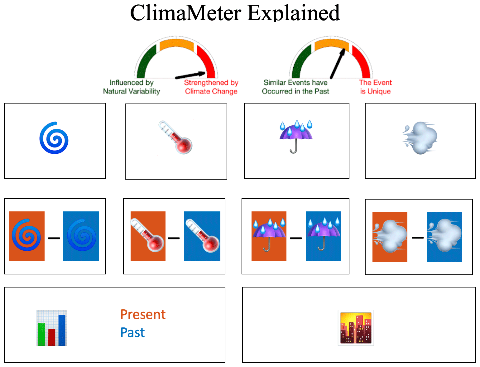
Figure 1 Schematic illustration of the ClimaMeter figure output. The top row of the figure consists of two gauge charts. The left-hand-side one indicates the respective roles of natural variability and climate change in explaining the changes detected. The right-hand-side gauge indicates the rarity of the surface-pressure pattern of the event. The second row provides a visual representation of the surface-pressure anomalies of the event and those of the hazard variables, i.e. temperature, precipitation, and wind speed. The third row provides maps of the composite differences between analogues in the present and past periods. The bottom row reports the seasonality of the analogues in each period (bottom-left panel) and detected changes in temperature, precipitation, and wind speed in three major urban areas within the analysis domain (bottom-right panel). See Sect. 2.2 for more details.

The top row of the figure consists of two gauge charts (Fig. 1, upper panels). The left-hand side indicates the respective roles of natural variability and climate change in explaining the changes detected in the event, i.e. “strengthened (for cold spells: weakened) by climate change” or “influenced by natural variability”. The right-hand gauge indicates the rarity of the surface-pressure pattern of the event (i.e. “the event is unique” or “similar events have occurred in the past”). The gauge representation is a visually immediate way to communicate this complex information. The gauge needles can take four positions: almost entirely to the left (5 %), two-thirds of the way to the left (35 %), two-thirds of the way to the right (65 %), or almost entirely to the right (95 %). These categories are determined based on the values of the underlying quantitative metrics (see below).

Furthermore, we provide visual representations of the surface-pressure anomalies of the event and of the hazard variables, i.e. temperature, precipitation, and wind speed (Fig. 1, panels in the second row). We also provide corresponding maps of the composite differences between analogues in the present and past periods (panels in the third row). Finally, we report the seasonality of the analogues in each period (Fig. 1, bottom-left panel) and detected changes in temperature, precipitation, and wind speed in three major urban areas within the analysis domain (bottom-right panel). The following explains Fig. 1 in more detail.

• 1.

  To determine the influence of natural variability or climate change on the event (left-hand gauge), we look at whether the analogues in the two periods occurred during significantly different phases of the ENSO, and/or the AMO, and/or the PDO. If none of the three modes shows significant differences between their distributions in the two periods, then the gauge points 95 % to the right. For each statistically significant difference in one of the variability modes, we shift the gauge 30 % to the left. Since we consider three modes, the gauge can thus have values of 95 %, 65 %, 35 %, or 5 %. We do not use 0 % or 100 % to acknowledge data and analysis uncertainties.

• 2.

  Concerning the rarity of the event in the data record (right-hand gauge), we use the analogue quality, Q, previously introduced in Faranda et al. (2022). Q is defined as the mean Euclidean distance from the event to its best analogues. This quantity is compared to Q_a, that is, the full distribution of Euclidean distances of the best analogues of the analogues of the event.

  • a.

    If for both the past and the present Q is below the 75th percentile of the distribution Q_a, the gauge points left (5 %). This means that similar events have occurred in the past.

  • b.

    If, instead, for both the past and the present periods Q is between the 75th and the 95th percentiles of Q_a, we assign the gauge to 35 %.

  • c.

    If for the past or the present Q is between the 75th and the 95th percentiles of Q_a, while for the other period it is above the 95th percentile, we assign the gauge to 65 %.

  • d.

    If Q exceeds the 95th percentile of Q_a for both the past and the present, we assign the maximum value to the gauge (95 %). This means that the event is largely unique in our dataset.

  We choose relatively high percentiles of Q_a to determine the positioning of the gauge since we analyse extreme events that, by their very nature, are not frequently observed. The gauge should therefore be interpreted as referring to events that in any case are comparatively unusual but that may not be unique. As with the other gauge, we do not use 0 % or 100 % to acknowledge data and analysis uncertainties.

• 3.

  We display the event's average surface-pressure anomaly, defined as the difference between the average surface pressure at each grid box in the selected region for the duration of the event and the average surface pressure at each grid box for the same calendar day(s) over the whole period of 1979–2022. The same is displayed for temperature, while absolute values are displayed for precipitation and wind speed.

• 4.

  We also display the difference between the average surface pressure for all analogues in the present period and the average surface pressure for all analogues in the past period. The same is done for the selected hazard variables. To determine significant changes between the two periods, we adopt a bootstrap procedure that consists of pooling the dates from the two periods together, randomly sampling 15 dates without replacement from this pool 100 times (higher values do not significantly change the results), and marking as significant only grid point changes larger than 2 standard deviations above or below the mean of the bootstrap sample. This is implemented for surface pressure in the summary figure and is highlighted in the report text.

Additional analyses are provided in Appendix A. These analyses are specifically intended for researchers and contain details that are fully understandable only by reading the methodology described in Faranda et al. (2022). They provide useful information such as the details of the hazard changes and the climate modes of variability highlighted in the report text.

3 Report-writing protocol

ClimaMeter has a structured protocol for writing reports that assess and contextualize extreme-weather events relative to climate change. This is a living document that can be updated based on input from the ClimaMeter core team. The latest version of the template at the time of writing, which is detailed in Appendix A, encompasses all aspects of the report, including the formulation of the report title, home page title (which appears on the https://www.climameter.org, last access: 12 July 2024, home page when the report is released), press summary, event description, climate and data background, ClimaMeter analysis, and conclusion.

The home page title categorizes extreme-weather events into those strengthened by human-driven climate change, mostly strengthened by human-driven climate change, likely influenced by both human-driven climate change and natural variability, or mostly driven by natural variability. This characterization was chosen to provide clear and immediate communication, even though we appreciate that there may be factors affecting the extremes which fall into neither category (for example human-driven land-use changes). In the report itself, the template starts with a press summary that provides context for the event, assesses its uniqueness, and characterizes it in terms of the role of climate change versus natural variability, based on the ClimaMeter analysis. The event description section details the specifics of the extreme-weather event including dates, location, impacts, and key meteorological characteristics. Links to relevant media reports are also provided. The event description ends with a simplified explanation of the atmospheric conditions leading to the extreme. The climate and data background section refers to Intergovernmental Panel on Climate Change (IPCC) reports and other relevant scientific information to provide context and support for the analysis. It also assesses the confidence level in the analysis based on the uniqueness of the event (right-hand gauge). A unique event is associated with low confidence since analogues will be poor; an event similar to others observed in the past gives us a higher confidence in the analogue-based analysis. The ClimaMeter analysis section examines changes in surface-pressure and hazard variables, comparing the present and past analogues to determine how the event has evolved between the two periods. It further evaluates the extent to which climate change may have strengthened the event (left-hand gauge). The conclusion provides a two-sentence summary of the analysis, summarizing the two gauges and the analogue composite difference maps. Overall, this protocol aims to offer an accessible yet comprehensive approach to assessing extreme-weather events in the context of climate change, prioritizing the clear communication of findings.

The report for a given extreme event is usually produced within 2–3 d of the event occurring, using the MSWX-NRT data if needed (see Sect. 2.1). When updated MSWX-Past data become available, we aim to update the report. Similarly, we update reports based on suggestions or criticisms that we receive, e.g. from colleagues or journalists, including correcting errors in the figures or analysis, modifying the text in response to requests for clarification, and updating estimates of the damage or of the meteorological measurements. In general, we strive to take into account any feedback that helps improve the reports. This means that we may update a given report several times. For every report, we indicate the first publication date, the date of the latest update, and the date when the report was finalized. Once the report is finalized, it cannot be changed further. After finalization, we aim to provide a PDF version of the report as well as a DOI citation. The finalization of the report may happen several months after the occurrence of the extreme event being analysed.

4 ClimaMeter event coverage and examples

Before 11 April 2024, ClimaMeter analysed 41 events. Figure 2 shows the geographical distribution of these events, the proportion of events for each hazard class, and the counts of events yielding specific values of the gauges. There are evident biases in the geographical homogeneity of events and hazards analysed since, as discussed, the event selection is guided by expert opinion and by the events' relevance to the general public. In the rest of this section, we present two examples to illustrate the ClimaMeter methodology in detail and its robustness with respect to changes in dataset (MSWX versus ERA5) and observables (mean sea-level pressure versus geopotential height in ERA5). The results and their presentation differ from the standard ClimaMeter reports and the protocol in Appendix A to provide a more thorough explanation of the methodology and also to better fit the requirements of a scientific paper. However, the content here is consistent with the corresponding ClimaMeter reports.

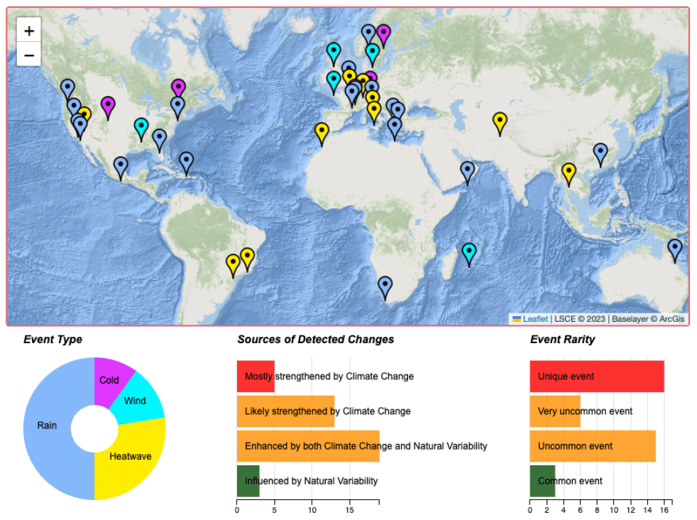
Figure 2 Screenshot of the event dashboard appearing on the ClimaMeter website, with extreme events analysed before 11 April 2024. See https://www.climameter.org/event-dashboard (last access: 12 July 2024).

4.1 21–23 August 2023 late summer French heatwave (30–52° N, 10° W–20° E)

4.1.1 Event description

Starting on 21 August, western and northern Europe experienced unusually high temperatures that peaked on 22 and 23 August. With a national temperature indicator of 27.5 °C, Wednesday, 23 August was the second-hottest day ever recorded in France (TF1 Info, 2023). A large number of daily maximum temperature records were broken in the country. In Toulouse, the thermometer reached 42.4 °C (previous record 40.7 °C); in Auch, 42.3 °C (previous record 40.9 °C); and in Narbonne, 42.1 °C (previous record 39.8 °C). Additionally, the heatwave was also extreme in mountainous areas, with Aiguille du Midi (∼ 3800 m a.s.l. in the Mont-Blanc massif) recording a maximum temperature over 10 °C. Finally, the minimum daily temperature of 30.4 °C in Menton set a new record for the minimum daily temperature in mainland France. The heatwave ended on 24 August, when cooler air from the Atlantic reached the country causing severe thunderstorms.

The heatwave was associated with a persistent area of high pressure (anticyclone) over western and central Europe against the background of a warm Atlantic ocean and warm Mediterranean sea and of a positive phase of the El Niño–Southern Oscillation. The surface-pressure anomaly (Fig. 3) pattern associated with the event consists of a high-pressure area over the Alps and central Europe and a low-pressure area over the south-eastern North Atlantic. Temperature anomalies show that temperatures were 7 to 10 °C warmer than usual for that time of the year over a large part of the domain considered (Fig. 3).

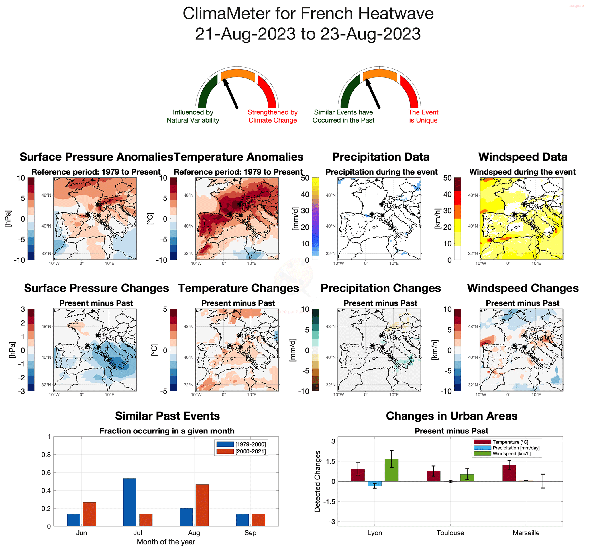
Figure 3 ClimaMeter output for the 21–23 August 2023 late-summer French heatwave based on MSWX data and with analogue selection based on surface-pressure anomalies. See Fig. 1 for an explanation of the different panels.

4.1.2 Climate and data background for the analysis

Chapter 11 of the IPCC AR6 report (Seneviratne et al., 2021) emphasizes that in western Europe there is strong evidence of an increase in maximum temperatures and in the frequency of heatwaves. Specifically, in western Europe, climate warming has already reached 1.7 °C compared to the pre-industrial era, with 1.5 °C of this increase occurring since the 1960s, particularly during the summer months. The number of heatwave days in western Europe has multiplied by 5, transitioning from an annual average of 2 d between 1960 and 2020 to about 10 d currently (Vautard et al., 2023).

Our analysis approach rests on looking for large-scale pressure patterns similar to those of the event of interest that have been observed in the past. For this event, we have medium-high confidence in the robustness of our approach given the available climate data, as the event is similar to other past events in the data record.

4.1.3 ClimaMeter analysis

Figure 3 reports ClimaMeter results for the late-summer French heatwave based on the MSWX dataset and how events similar to this have changed in the present (2001–2022) compared to what they would have looked like if they had occurred in the past (1979–2000) in the region of 30–52° N, 10° W–20° E. Surface-pressure changes show that the pressure over Brittany has become higher, while it has become lower over Italy. We underline that such changes are rather modest. Temperature changes show that similar events produce temperatures that in the present climate are between 0 and 2 °C hotter than what they would have been in the past, especially in the Mediterranean area. This coincided with temperatures in Lyon, Toulouse, and Marseille being over 1 °C hotter than what they would have been in the past. We also note that similar past events have become more common in the month of August, while they previously occurred largely in July. However, the differences in average maximum temperatures between these 2 months are limited in many French cities.

Finally, we find that sources of natural climate variability (see Fig. A1), notably the Pacific Decadal Oscillation and Atlantic Multidecadal Oscillation, may have influenced the event. This suggests that the changes we see in the event compared to the past may be partly due to human-driven climate change, with a contribution from natural variability.

4.1.4 Conclusions

Based on the above, we conclude that heatwaves similar to the late August 2023 French heatwave have become between 0 and 2 °C warmer in the present than in the past. We interpret this heatwave as an event for which natural climate variability played a role.

4.1.5 Comparison with ERA5 data

In addition to the above report, which mostly follows the ClimaMeter protocol, we discuss here the results obtained with ERA5 data, to assess the robustness of the method (cf. Fig. 3 with Fig. 4). Temperature changes are largely geographically consistent across the two datasets, albeit more intense in ERA5. Precipitation changes are also consistent, apart from small variations over the Alps likely due to the higher spatial resolution of MSWX (0.1° × 0.1°) compared to ERA5 (0.25° × 0.25°). Wind speed changes also match, apart from small local differences in parts of northern Italy. The seasonality of similar past events for both datasets indicates more frequent events in August and a decreased frequency in July. Changes in the selected urban areas are consistent across the two datasets in terms of temperature – although, again, ERA5 indicates larger temperature differences than MSWX – while some discrepancies are observed in wind speed changes. Finally, while the indications of the uniqueness of the event match (right-hand gauge plots in Figs. 3, 4), there is a difference in the role of natural variability, with ERA5 pointing towards a weaker role of the latter driven only by the Pacific Decadal Oscillation. Reasonable agreement is also confirmed when searching analogues using ERA5 500 hPa geopotential height (z₅₀₀, Fig. 5), although in this case we see clear differences in the seasonality results as well as in both the uniqueness and natural variability gauges.

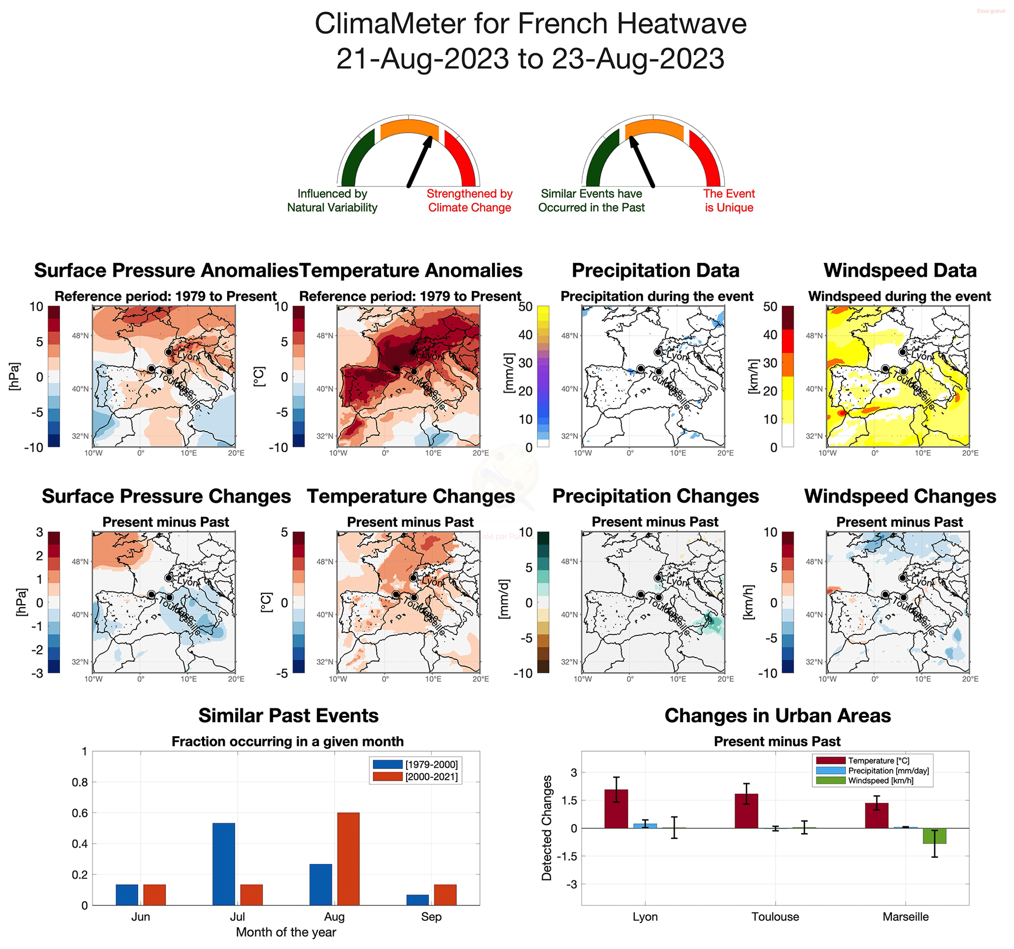
Figure 4 ClimaMeter output for the 21–23 August 2023 late-summer French heatwave based on ERA5 data and with analogue selection based on sea-level pressure anomalies. See Fig. 1 for an explanation of the different panels.

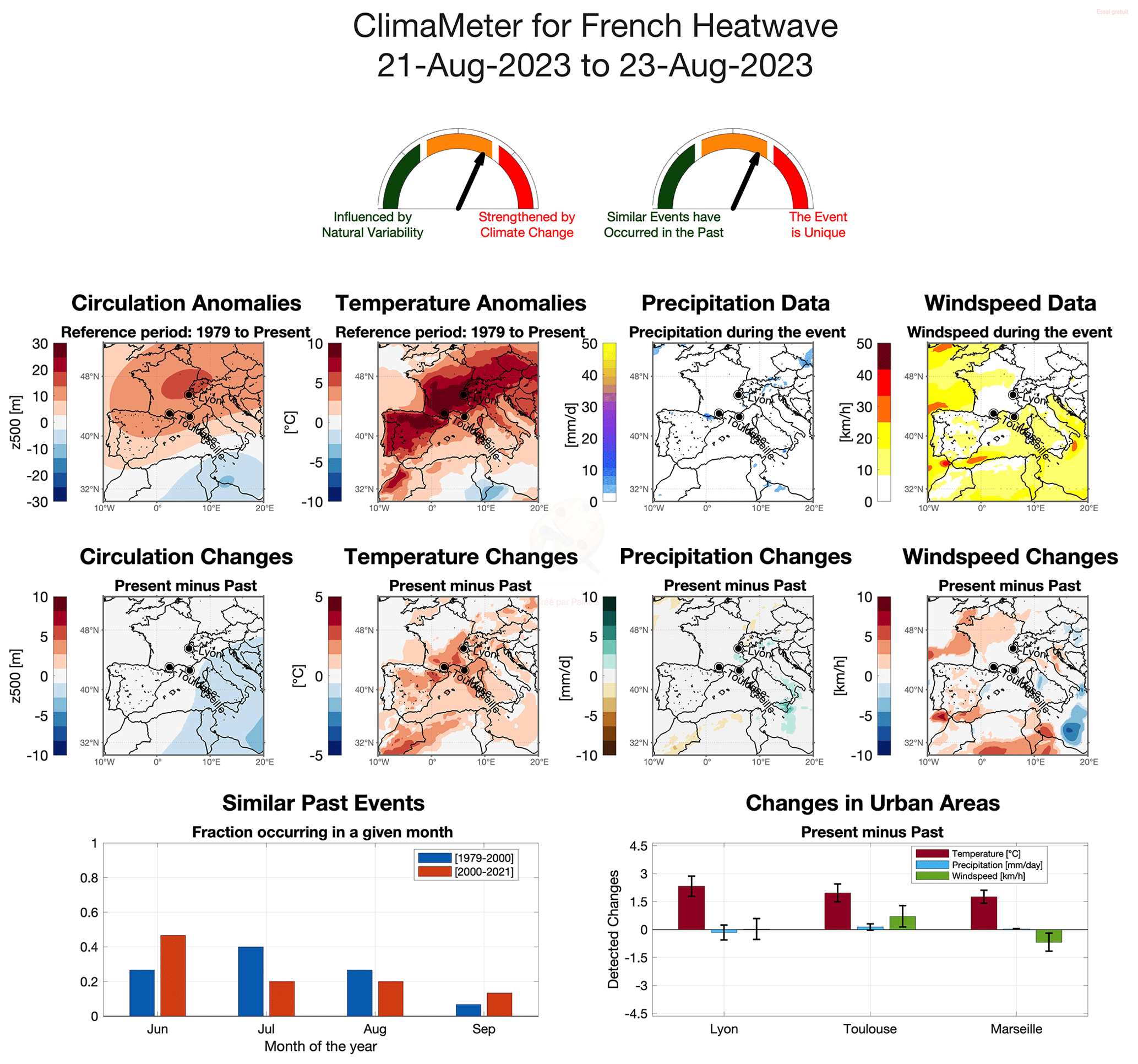
Figure 5 ClimaMeter output for the 21–23 August 2023 late-summer French heatwave based on ERA5 data and with analogue selection based on 500 hPa geopotential height anomalies (z₅₀₀). See Fig. 1 for an explanation of the different panels.

4.2 5 July 2023 Storm Poly in northern Europe (46–60° N, 0–25° E)

4.2.1 Event description

On 5 July 2023, an extratropical storm named Poly hit Germany, the Netherlands, and Denmark, causing significant damage and resulting in two casualties. It featured hurricane-force wind gusts up to 146 km h⁻¹ locally, the strongest ever recorded for a summer storm in the Netherlands (EUMETSAT, 2023). The storm's rapid cyclogenesis began over the North Atlantic. Once it made landfall, severe winds were accompanied by heavy rainfall and led to uprooted trees and transportation disruptions. The majority of severe weather reports associated with the storm concerned severe wind. Storm Poly displayed clear negative surface-pressure anomalies over the Netherlands, Denmark, and parts of north-western Germany, while wind speed during the storm in the MSWX data we used for analysis was around or above 30–40 km h⁻¹ over a large swath of the Baltic and northern Europe (Fig. 6).

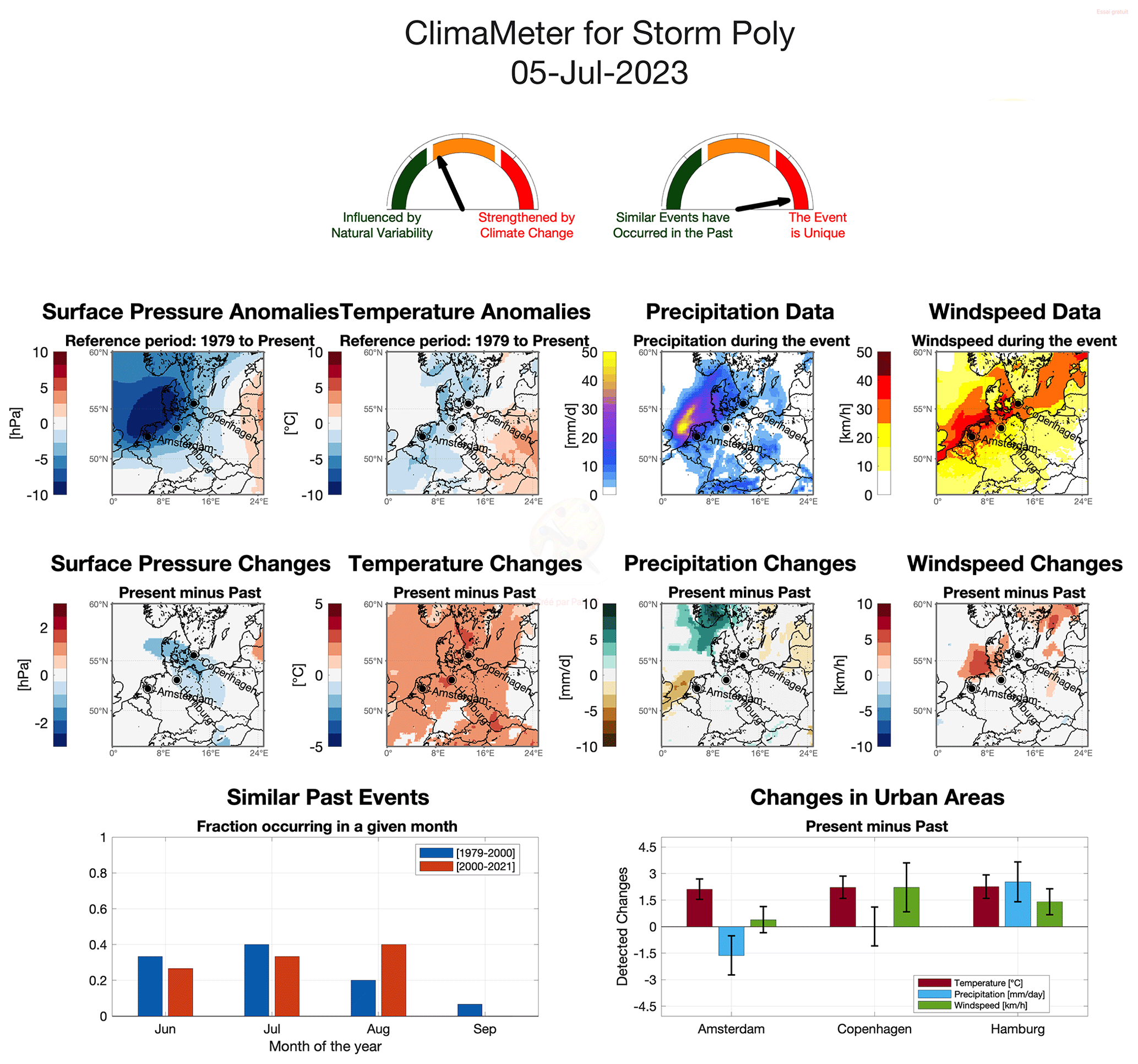
Figure 6 ClimaMeter output for the 5 July 2023 Storm Poly in northern Europe based on MSWX data and with analogue selection based on surface-pressure anomalies. See Fig. 1 for an explanation of the different panels.

4.2.2 Climate and data background for the analysis

Chapter 11 of the IPCC AR6 report (Seneviratne et al., 2021) highlights that there is low confidence in recent total extratropical storm changes globally but medium confidence in a poleward storm track shift since the 1980s. Understanding past-century extratropical storm trends is hindered by interannual variability and variations in the assimilated data, particularly when moving from the pre-satellite era to the satellite era. Data for the Northern Hemisphere support decreased central pressure for cyclones (<970 hPa) in summer and winter during 1979–2010 but with non-monotonic trends. The background mean sea-level pressure seasonal and regional variations complicate assessing extratropical storm intensity trends based on absolute central pressure.

For Poly, we have low confidence in the robustness of our approach given the available climate data, as the event is largely unique in the data record. Indeed, the identified analogues consist of low-pressure systems with weaker anomalies or were spatially displaced with respect to Poly.

4.2.3 ClimaMeter analysis

Figure 6 reports ClimaMeter results for Storm Poly and how events similar to this have changed in the present (2001–2022) compared to what they would have looked like if they had occurred in the past (1979–2000). The surface-pressure changes show that the pressure over the area affected by the storm has become lower, indicating deeper cyclones in the present period than in the past. Wind speed changes show that similar events produce winds between 2 and 6 km h⁻¹ stronger than what they would have been in the past, consistent with the surface-pressure changes. Storms similar to Poly are associated with stronger winds in Hamburg (Germany) and Copenhagen (Denmark) than they would have been in the past. We also note that similar past events have become more common in the month of August, while they previously occurred more in other summer months (peaking in July) or even in September. Finally, we find that sources of natural climate variability (Figs. 6 and A4, A5, A6), notably the Atlantic Multidecadal Oscillation and the Pacific Decadal Oscillation, may have partly influenced the event. This suggests that the changes we see in the event compared to the past may be partly due to human-driven climate change, with a contribution from natural variability.

4.2.4 Conclusions

Based on the above, we conclude that storms similar to Poly display lower pressure and stronger winds in the present than in the past. We interpret this storm as a largely unique event for which natural climate variability played a role.

4.2.5 Comparison with ERA5 data

As for the previous example, we provide, in addition to the ClimaMeter report, a comparison with ERA5 data to assess the robustness of the method (cf. Figs. 6 and 7). We again find overall good agreement yet with some differences – for example in the observed wind speed changes between present and past events in the selected urban areas. Nonetheless, both datasets present consistent spatial patterns for wind speed and surface-pressure changes over the region affected by the storm, which are the key conclusions that we draw from our analysis. The main difference emerges when comparing the gauge plots, showing that for the ERA5 analogues the footprint of climate change is stronger than for the MSWX ones. Moreover, in the MSWX data the event is unique, while in the ERA5 data it is a more common event. This difference can be related to the cyclonic pattern that appears to be more spatially extended in ERA5 over the North Atlantic, leading to the selection of different analogues. The conclusion of an increase in wind speed also holds when searching for analogues using the 500 hPa geopotential height from ERA5 (z₅₀₀, Fig. 8). In this case, however, the difference in the right-hand gauge relative to MSWX is even more marked, with ERA5 indicating that events similar to the one being studied have occurred in the past.

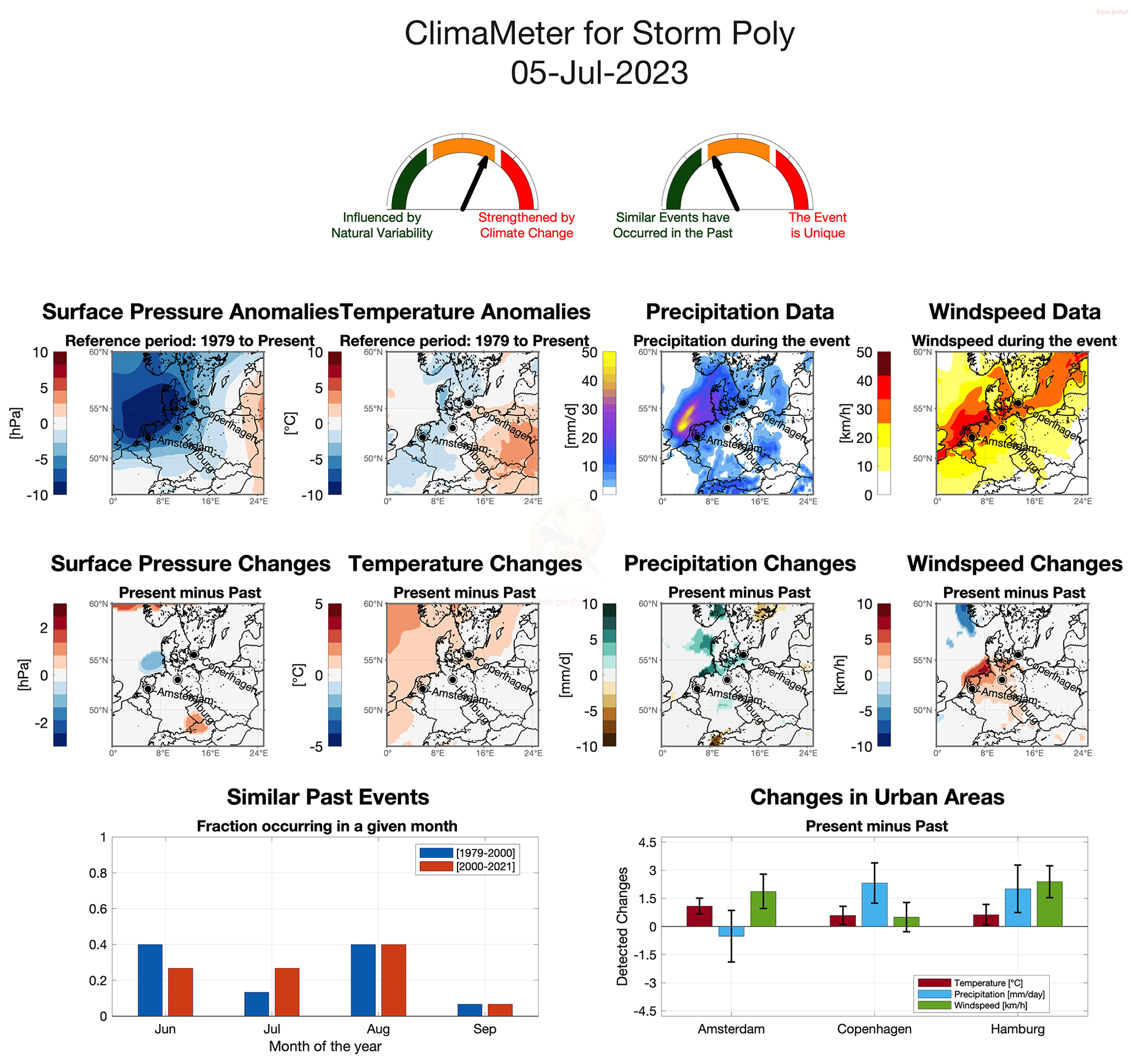
Figure 7 ClimaMeter output for the 5 July 2023 Storm Poly in northern Europe based on ERA5 data and with analogue selection based on sea-level pressure anomalies. See Fig. 1 for an explanation of the different panels.

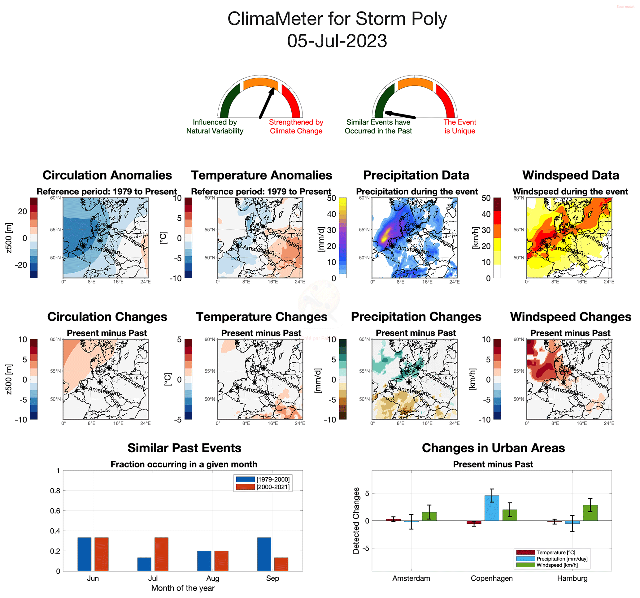
Figure 8 ClimaMeter output for the 5 July 2023 Storm Poly in northern Europe based on ERA5 data and with analogue selection based on 500 hPa geopotential height anomalies (z₅₀₀). See Fig. 1 for an explanation of the different panels.

4.3 Statistics of events

Figure 9 presents a statistical summary of the extreme events analysed by ClimaMeter before 11 April 2024. We specifically highlight the average values of the two gauges representing the respective influences of natural variability and climate change on the selected events and the uniqueness of the events, as well as a summary of the possible role of modes of natural variability. These insights are provided for all events collectively, as well as separately for each hazard class: cold spells, heatwaves, heavy rainfall, and wind storms.

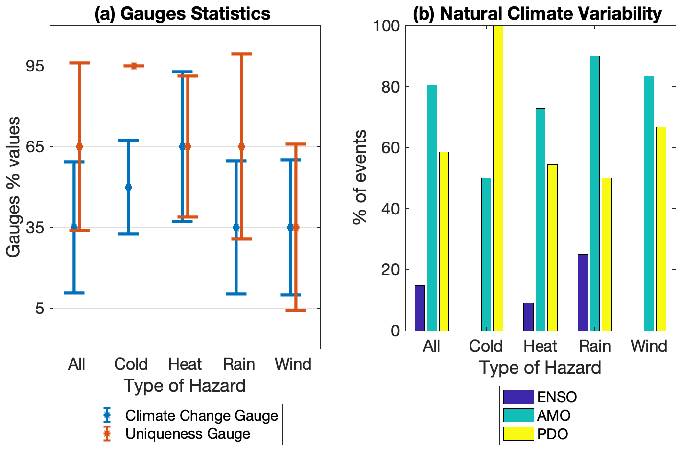
Figure 9 The interval bars show the median percentage values (circles) and the standard deviation (whiskers) of ClimaMeter's climate change and uniqueness gauges (a), while the bars show the percentage of events that may have been affected by shifts in a given large-scale mode of climate variability (b). The figure presents both bulk statistics for all events (41 in total) and statistics for the individual hazard classes: cold spells (4 events), heatwaves (11 events), heavy rainfall (20 events), and wind storms (6 events).

Overall, we observe that the median percentage value of the uniqueness gauge is 65 %, indicating that the majority of events that we analyse lack similar past analogues. This is not necessarily surprising given that extreme events are by definition rare. Conversely, the median climate change gauge value of 35 % suggests that the occurrence and characteristics of many events can be at least partially explained by modes of natural variability rather than by climate change alone. In this respect, we however note that we take a restrictive approach to quantifying this, as discussed in Sect. 5. Upon closer examination of specific hazards, it is noteworthy that all cold-spell events in our dataset are unique (gauge value of 95 %). Perhaps unsurprisingly, the anthropogenic climate change signal is most visible in heatwaves, in line with the latest IPCC report (see in particular Fig. SPM.3 in Seneviratne et al., 2021).

Concerning the modes of large-scale climate variability, we find a dominant role of the Atlantic Multidecadal Oscillation (AMO), with the Pacific Decadal Oscillation (PDO) playing a secondary role and the El Niño–Southern Oscillation (ENSO) contributing less. Interestingly, the PDO influences all cold-spell events, while the AMO dominates in all other hazard categories. These results are, however, likely to be heavily influenced by the geographical distribution of the events analysed by ClimaMeter.

These findings offer an insight into the interplay between climate change, natural variability, and specific hazards. However, given the small sample size and inhomogeneous geographical coverage of the analysed events (Fig. 2), the above statistics may not be indicative of the global statistics of the selected natural-hazard classes.

5 Conclusions

ClimaMeter is an effort to contextualize the ever-increasing occurrence of extreme and hazardous weather events across the globe relative to ongoing human-driven climate change. Together with other international efforts to rapidly communicate climate change, such as the World Weather Attribution, the Climate Shift index, and the C3S Copernicus programme, ClimaMeter responds to a pressing need to enhance the way we communicate on this critical issue to the general public and to provide a new tool for policymakers who face the implications of climate change. ClimaMeter's framework is flexible and is not restricted to a specific region or event, as evidenced by the coverage displayed in Fig. 2.

At the heart of ClimaMeter's approach lies an analysis of weather conditions similar to those that caused the extreme event of interest (so-called atmospheric circulation analogues), which are diagnosed using surface pressure. The analysis then leverages analogues to diagnose changes over time in four key meteorological hazard indicators: rainfall, wind speed, and high or low temperatures. These, combined with the analysis of the circulation analogues, serve as the cornerstone for understanding and contextualizing the dynamics of the analysed extreme-weather phenomena.

We see the rapidity and reproducibility of the ClimaMeter framework as two of its key strengths. Indeed, ClimaMeter reports typically become available only a few days after the occurrence of the extreme event of interest and rely on publicly accessible datasets rather than on ad hoc numerical simulations. Nonetheless, we also recognize some limitations of the framework. One is that the choice to limit our analysis to the satellite era (post 1979) limits the length of the available climatic time series and thus the statistical robustness of our analysis. A second limitation is given by the choice to reduce the assumed influence of climate change by 30 % each time a significant difference is detected in a mode of natural variability between the analogues we select in the past and present periods for the event being analysed. By doing this, we risk underestimating the role of climate change since the contributions of a mode of climate variability and of climate change to a given extreme event are not mutually exclusive. Another important caveat is that we adopt a simplified approach to determine the role of natural climate variability that does not account for the geographical location of the extreme event of interest. A further methodological limitation is that we do not estimate quantitatively the effects of climate change and natural variability on the physical characteristics of a given extreme event, contrary to probabilistic approaches for extreme event attribution. The comparison between ERA5 sea-level pressure and geopotential height analogues and the MSWX surface-pressure analogues has revealed that the diagnosed changes in meteorological hazards are geographically consistent across datasets and variables. However, there may be variations in the magnitude of the changes, and ClimaMeter gauges may take different values for the different datasets. In our analysis, we have further encountered instances where there is a discrepancy between the near-real-time MSWX data and the definitive (called past in the MSWX archive) data used for report updates. This underscores the importance of not regarding ClimaMeter's rapid assessments as replacements for peer-reviewed research but rather as initial evaluations of extreme events immediately following their occurrence.

Related to this, we also reiterate that the spatial domain used for the analogues is chosen based on expert judgement from members of the ClimaMeter project, and therefore it carries an arbitrary component. The results of a ClimaMeter analysis are likely to provide different results if different domains are chosen, especially if larger- or smaller-scale features become dominant due to a much larger or smaller domain. Furthermore, we stress that there are limits to the analogue approach. For example, conclusions about the impact of climate change are more robust in case studies where the analogue quality is high and where the long-term climate trends match the changes in the extreme event analogues themselves. Finally, ClimaMeter is designed to work for extreme events whose dynamics can be well represented through circulation analogues. Small-scale events where local processes are important – e.g. an isolated tornado or a hail storm – are currently outside the scope of ClimaMeter.

Amidst the escalating challenges posed by climate change, ClimaMeter holds potential as a valuable tool for various stakeholders. Researchers can utilize ClimaMeter’s methodology to delve into the relationship between climate change and specific extreme events, even those not typically addressed in statistical attribution studies, such as medicanes, explosive extratropical cyclones, tropical cyclones, acqua alta events in Venice, and others. For instance, building upon insights from Figs. 2 and 9, further investigation can deepen our understanding of how climate variability influences specific hazard classes. While the statistics presented offer a glimpse into this relationship, a more comprehensive approach could involve extending the analysis to encompass all events detected within a certain hazard category and geographic region. As an example, focusing on windstorms in Europe by leveraging datasets such as the one compiled by Faranda et al. (2023) could provide a wealth of data to investigate the influence of climate variability on this class of extreme events in a more nuanced manner. Policymakers can rely on the rapidity of ClimaMeter for an initial evaluation of the extent to which specific extreme event categories in a given geographical area are affected by climate change, thus providing a knowledge basis for addressing the growing risks and vulnerabilities associated with extreme events. The rapid ClimaMeter reports can then be compared to other attribution frameworks where there are sufficient resources to implement these for large numbers of events. Finally, the general public can benefit from ClimaMeter's accessible and informative approach, fostering greater awareness and understanding of the urgency and complexity of climate change and its consequences. This occurs both directly through ClimaMeter's website and social media and indirectly through the media reports on ClimaMeter analyses.

Ultimately, we hope that frameworks like ClimaMeter may be a small but important piece in the puzzle to achieve a more resilient and sustainable climate future by integrating scientific research, communication, and operational implementation.

Appendix A: ClimaMeter template for reports

A1 Template for report titles

For the report titles we use the following formulations. We have removed the case of cold spells here to make the text easier to follow.

• “Heavy precipitation/high temperatures/strong winds” in “location name” was/were strengthened by human-driven climate change (if both gauge indicators are on red).

• “Heavy precipitation/high temperatures/strong winds” in “location name” was/were mostly strengthened by human-driven climate change (if one of the gauge indicators is on red and the other is on yellow).

• “Heavy precipitation/high temperatures/strong winds” in “location name” was/were likely influenced by both human-driven climate change and natural variability (if both gauge indicators are on yellow or one is on green and one on yellow).

• “Heavy precipitation/high temperatures/strong winds” in “location name” was/were mostly driven by natural variability (if both gauge indicators are on green).

• Low confidence prevents ascribing “heavy precipitation/high temperatures/strong winds” in “location name” to human-driven climate change (if the left gauge indicator is on green and the right gauge indicator is on red or when detected changes are not aligned with the existing literature).

A2 Press summary

For the first sentence about changes in the event intensity, the text is as follows.

• “Event type” similar to “event name” is/are “change here” in the present than it would have been in the past “geographical area here” (example: cold spells similar to Borea are 2 °C warmer in the present than they would have been in the past across all of northern Europe).

For the second sentence about the uniqueness of the event, the text is as follows.

• “Event name” was a largely unique event (if the arrow on the right-hand gauge points to the right).

• “Event name” was a very uncommon event (if the arrow on the right-hand gauge points three-quarters to the right).

• “Event name” was a somewhat uncommon event (if the arrow on the right-hand gauge points three-quarters to the left).

• “Event name” was similar to several events in the past (if the arrow on the right-hand gauge points to the left).

For the third sentence about the role of climate change versus natural variability, the text is as follows.

• We ascribe the “high/low/heavy/strengthened” “variable name here” of/associated with “event name” to human-driven climate change, and natural climate variability likely played a minor role (if the arrow on the left-hand gauge points to the right).

• We mostly ascribe the “high/low/heavy/strengthened” “variable name here” of “event name” to human-driven climate change, and natural climate variability likely played a modest role (if the arrow on the left-hand gauge points three-quarters to the right).

• Natural climate variability likely played a role in driving the pressure pattern and the associated “increase/decrease” in “variable name here” linked to “event name”, but human-driven climate change has also contributed (if the arrow on the left-hand gauge points three-quarters to the left).

• Natural climate variability likely played an important role in driving the pressure pattern and the associated “increase/decrease” in “variable name here” linked to “event name” (if the arrow on the left-hand gauge points to the left).

A3 Event description

“On/starting from/in the period” “date(s)” “location” experienced “brief description of event, ideally with some numbers” (example of the description: unusually low temperatures for the season, with −20 °C being recorded in Stockholm. These frigid temperatures were part of a broader area of below-average temperatures, peaking in the first week of December and stretching from Scandinavia all the way to southern France). The “event type”/during “event name or similar” “brief description of the atmospheric configuration for laypeople” (example: during the Scandinavian cold spell of November 2022, the surface-pressure anomaly pattern displayed a large high-pressure area over the North Atlantic, drawing cold arctic and Siberian air over the continent. The presence of low pressure over central Europe further favoured cold-air advection. This resulted in temperature anomalies of up to 10° below average. The high-pressure area in the North Atlantic persisted until early December, after which warmer air masses from the North Atlantic spread over large parts of Europe). It is important that the event description refers to both panels in the first row of maps and uses the panel titles to refer to them, i.e. surface-pressure anomaly pattern, temperature anomalies, wind speed, or precipitation.

A4 Climate and data background for the analysis

“According to the/in chapter XX of the” IPCC AR6 report “brief summary of confidence level for change in frequency/intensity of the selected extreme” (example: it is virtually certain that there has been a decrease in severity and/or frequency of cold spells in the last several decades, and the consensus is that at a global level this decrease will continue in the future.). “Additional information about specific location/event type if relevant” (example: in Scandinavia, cold spells have become on average 4 °C warmer since 1950). Our analysis approach rests on looking for weather situations similar to those of the event of interest that have been observed in the past.

• For “event name”, we have “high confidence in the robustness of our approach given the available climate data, as the event is very similar to other past events in the data record” (if the right-hand gauge points to the left).

• For “event name”, we have “medium-high confidence in the robustness of our approach given the available climate data, as the event is similar to other past events in the data record” (if the right-hand gauge points three-quarters to the left).

• For “event name”, we have “medium-low confidence in the robustness of our approach given the available climate data, as the event is unusual in the data record” (if the right-hand gauge points three-quarters to the right).

• For “event name”, we have “low confidence in the robustness of our approach given the available climate data, as the event is largely unique in the data record” (if the right-hand gauge points to the right).

A5 ClimaMeter analysis

We analyse here (see methodology for more details) how events similar to “event name” have changed in the present (2001–2022) compared to what they would have looked like if they had occurred in the past (1979–2000). Surface-pressure changes show “brief description of the changes here” (example: that high pressure over the North Atlantic has become weaker than in the past, resulting in weaker cold-air advection over Europe). “Temperature changes/precipitation changes/wind changes” show that similar events produce “variable name here” that in the present climate are “brief description of the changes here” (example: temperatures that in the present climate are between 1 and 4 °C hotter than what they would have been in the past). “This has resulted in/this coincided with/similar connective phrase” “description of variable changes over cities as shown in figure” than they would have been in the past (example: temperatures in Berlin and Stockholm having become between 3 and 4 °C warmer than they would have been in the past). We also note that similar past events “description of seasonal changes in occurrence of the analogues” (example: have become more common in the spring than in the winter months, contributing to making the cold spells less severe).

• Finally, we find that sources of natural climate variability, notably the “Pacific Decadal Oscillation/El Niño–Southern Oscillation/Atlantic Multidecadal Oscillation”, may have heavily influenced the event. This means that the changes we see in the event compared to the past may be primarily due to natural climate variability (if the left-hand gauge points to the left).

• Finally, we find that sources of natural climate variability, notably the “Pacific Decadal Oscillation/El Niño–Southern Oscillation/Atlantic Multidecadal Oscillation”, may have influenced the event. This suggests that the changes we see in the event compared to the past may be partly due to human-driven climate change, with a contribution from natural variability (if the left-hand gauge points three-quarters to the left).

• Finally, we find that sources of natural climate variability, notably the “Pacific Decadal Oscillation/El Niño–Southern Oscillation/Atlantic Multidecadal Oscillation”, may have only partly influenced the event. This means that the changes we see in the event compared to the past may be mostly due to human-driven climate change (if the left-hand gauge points three-quarters to the right).

• Finally, we find that sources of natural climate variability did not influence the event. This means that the changes we see in the event compared to the past may be primarily due to human-driven climate change (if the left-hand gauge points to the right).

A6 Conclusion

Based on the above, we conclude that “event type” similar to “event name” have/has become “short description of how the circulation change likely affected the intensity of the event” (example: have become 3 °C warmer than in the present than in the past). We interpret “event name” as

• a largely unique event (if the right-hand gauge points to the right),

• an unusual event (if the right-hand gauge points three-quarters to the right),

• an event (if the right-hand gauge points three-quarters to the left or to the left).

The following text should be connected to the previous text as appropriate:

• whose characteristics can be ascribed to human-driven climate change (if the arrow on the left-hand gauge points to the right),

• whose characteristics can mostly be ascribed to human-driven climate change (if the arrow on the left-hand gauge points three-quarters to the right),

• for which natural climate variability played a role (if the arrow on the left-hand gauge points three-quarters to the left),

• for which natural climate variability likely played an important role (if the arrow on the left-hand gauge points to the left).

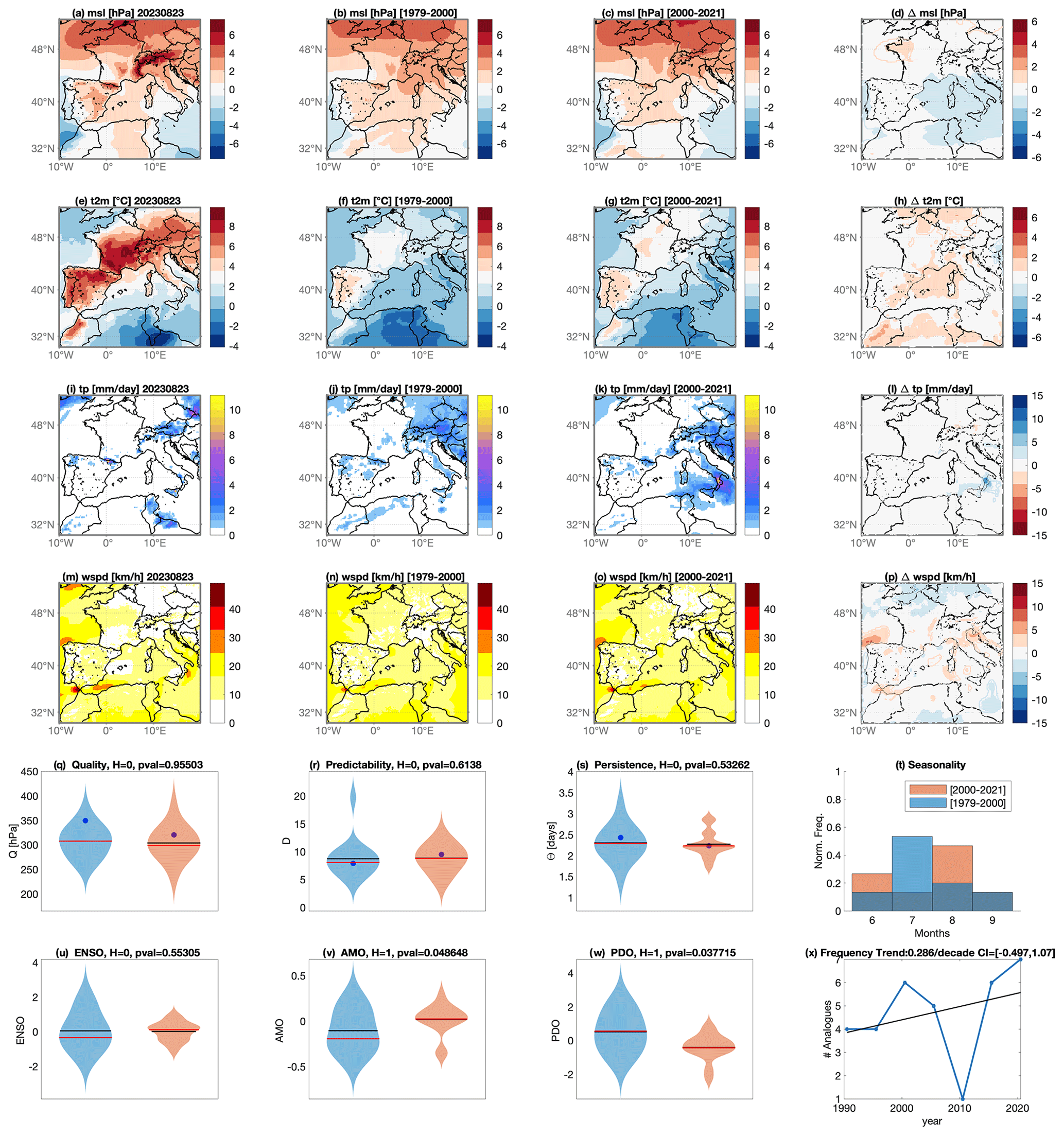
Figure A1 The 21–23 August 2023 late-summer French heatwave. Average surface-pressure anomalies (msl) (a), average 2 m temperatures anomalies (t2m) (e), cumulated total precipitation (tp) (i), and average wind speed (wspd) (m) during the event. Average of the surface-pressure analogues found in the counterfactual (1979–2000) (b) and factual (2000–2021) periods (c) along with corresponding 2 m temperatures (f, g), cumulated precipitation (j, k), and wind speed (n, o). Changes between present and past analogues for surface pressure (Δmsl) (d), 2 m temperatures (Δt2m) (h), cumulated total precipitation (Δtp) (l), and wind speed (Δwspd) (p). Colour-filled areas indicate significant anomalies with respect to the bootstrap procedure described in Sect. 2. Violin plots for the past (blue) and present (orange) periods for analogue quality Q and analogue quality distribution Q_a (q), predictability index D (r), persistence index Θ (s), and distribution of analogues in each month (t). Violin plots for the past (blue) and present (orange) periods for ENSO (u), AMO (v), and PDO (w). Number of the analogues occurring in each sub-period (blue) and the linear trend (black) (x). Horizontal bars in panels (q)–(s) and (u)–(w) correspond to the mean (black) and median (red) of the distributions. Values for the peak day of the extreme event are marked by a blue dot. The date indicated in the plot titles refers to the last day of the event.

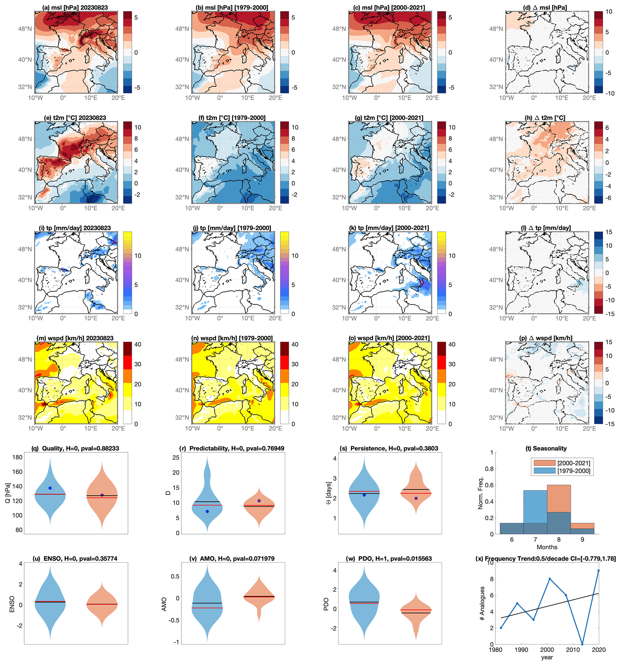
Figure A2 The 21–23 August 2023 late-summer French heatwave. As in Fig. A1 but for ERA5 sea-level pressure data.

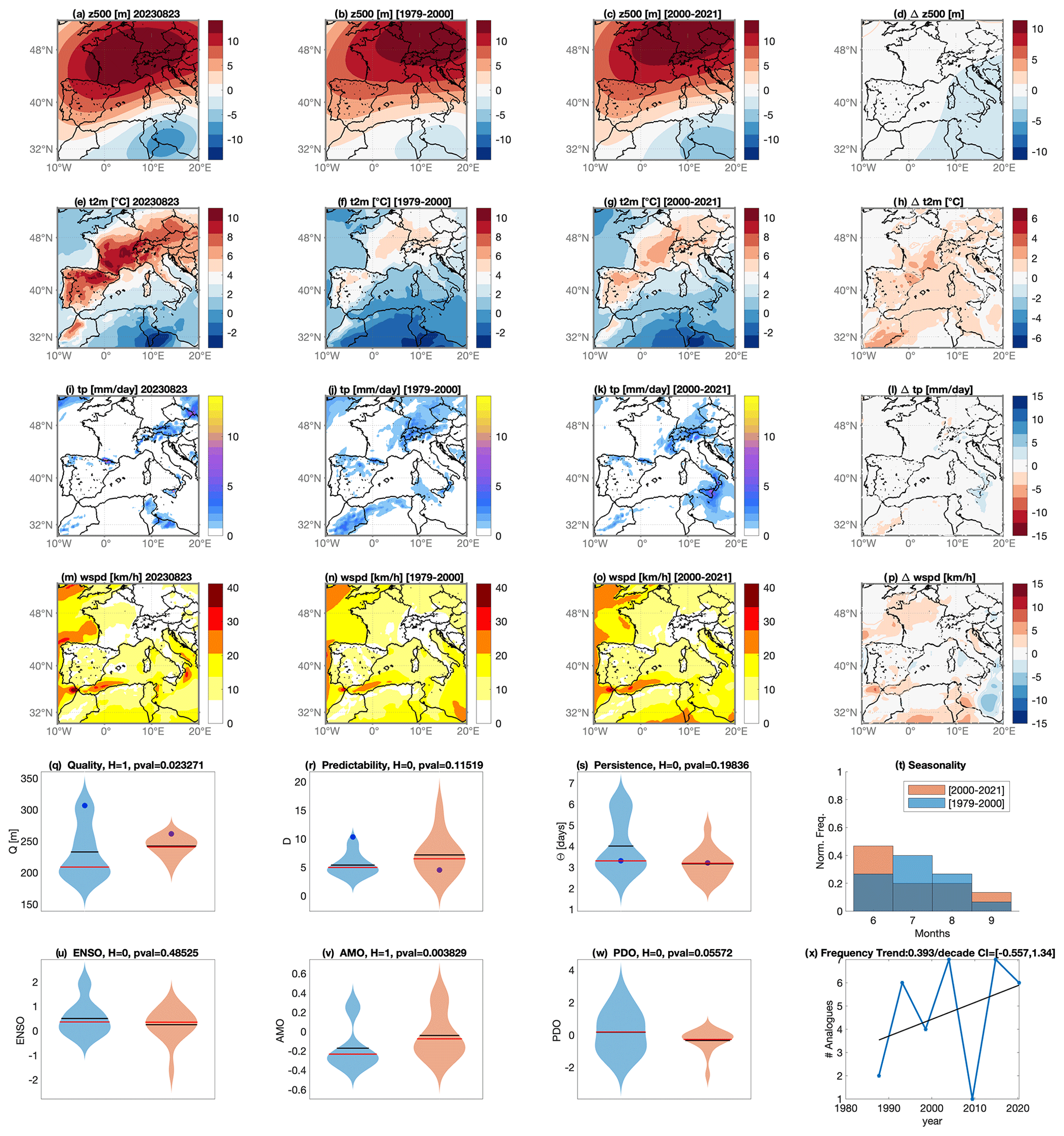
Figure A3 The 21–23 August 2023 late-summer French heatwave. As in Fig. A1 but for ERA5 500 hPa geopotential height (z₅₀₀) data.

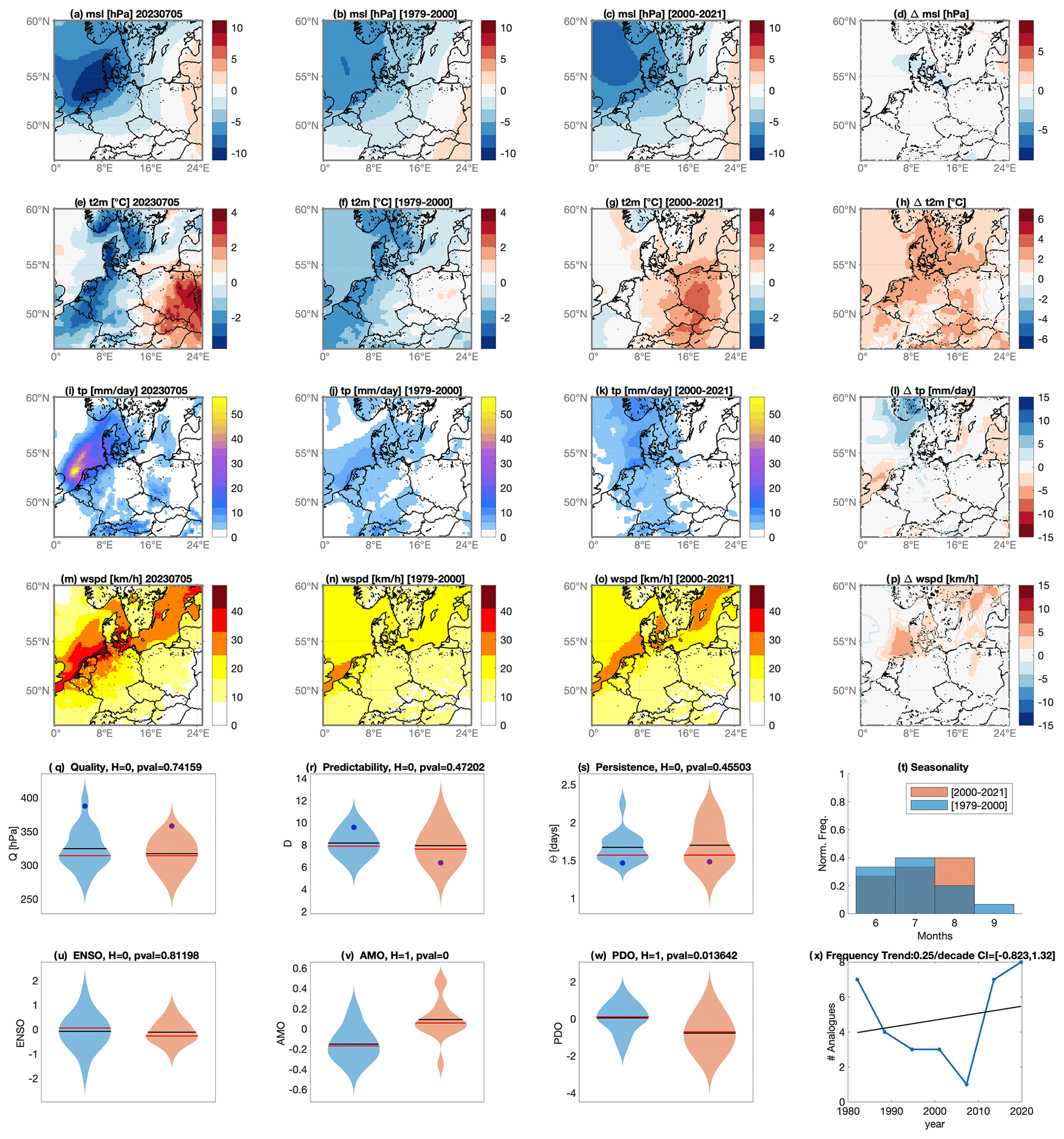
Figure A4 As in Fig. A1 but for the 5 July 2023 Storm Poly in northern Europe.

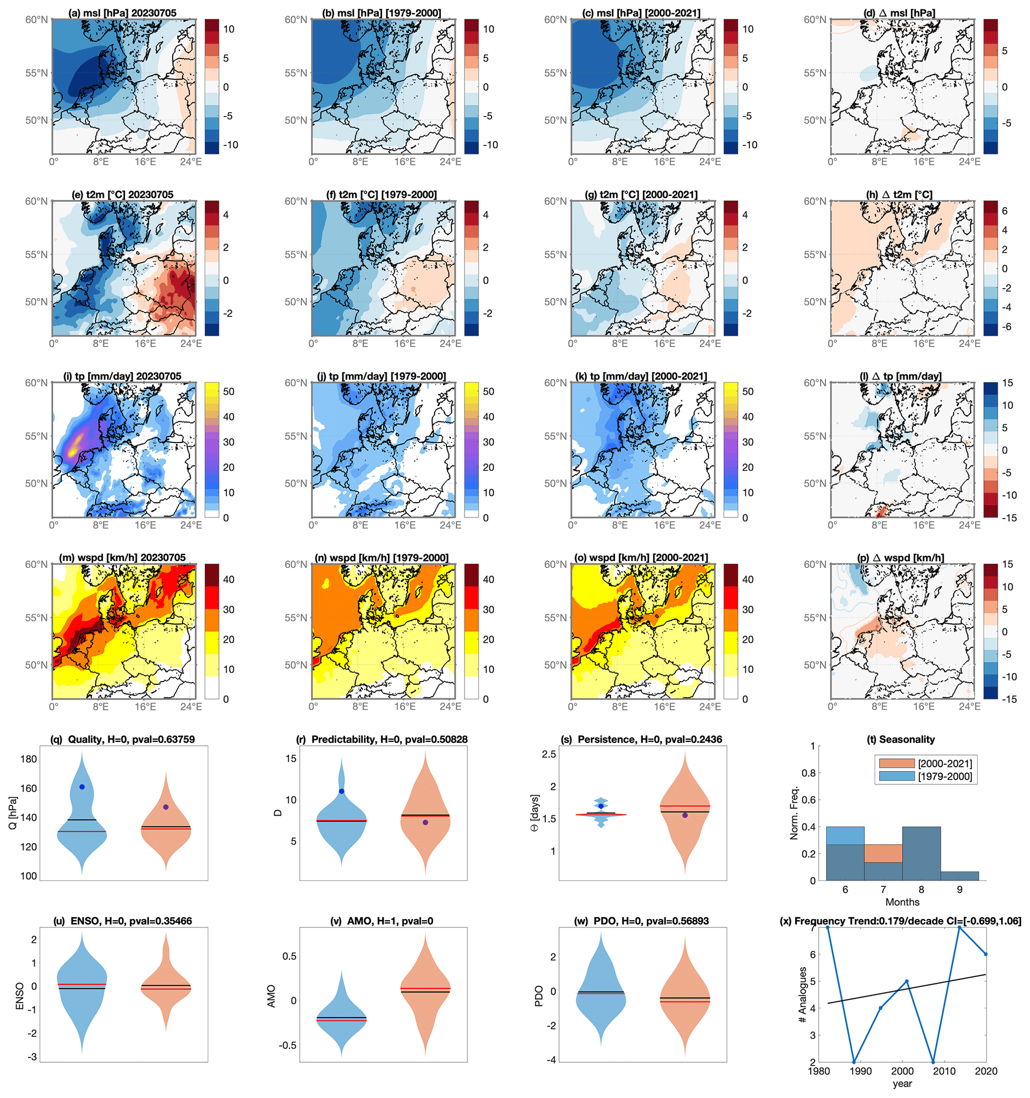
Figure A5 Storm Poly in northern Europe on 5 July 2023. As in Fig. A4 but for ERA5 sea-level pressure data.

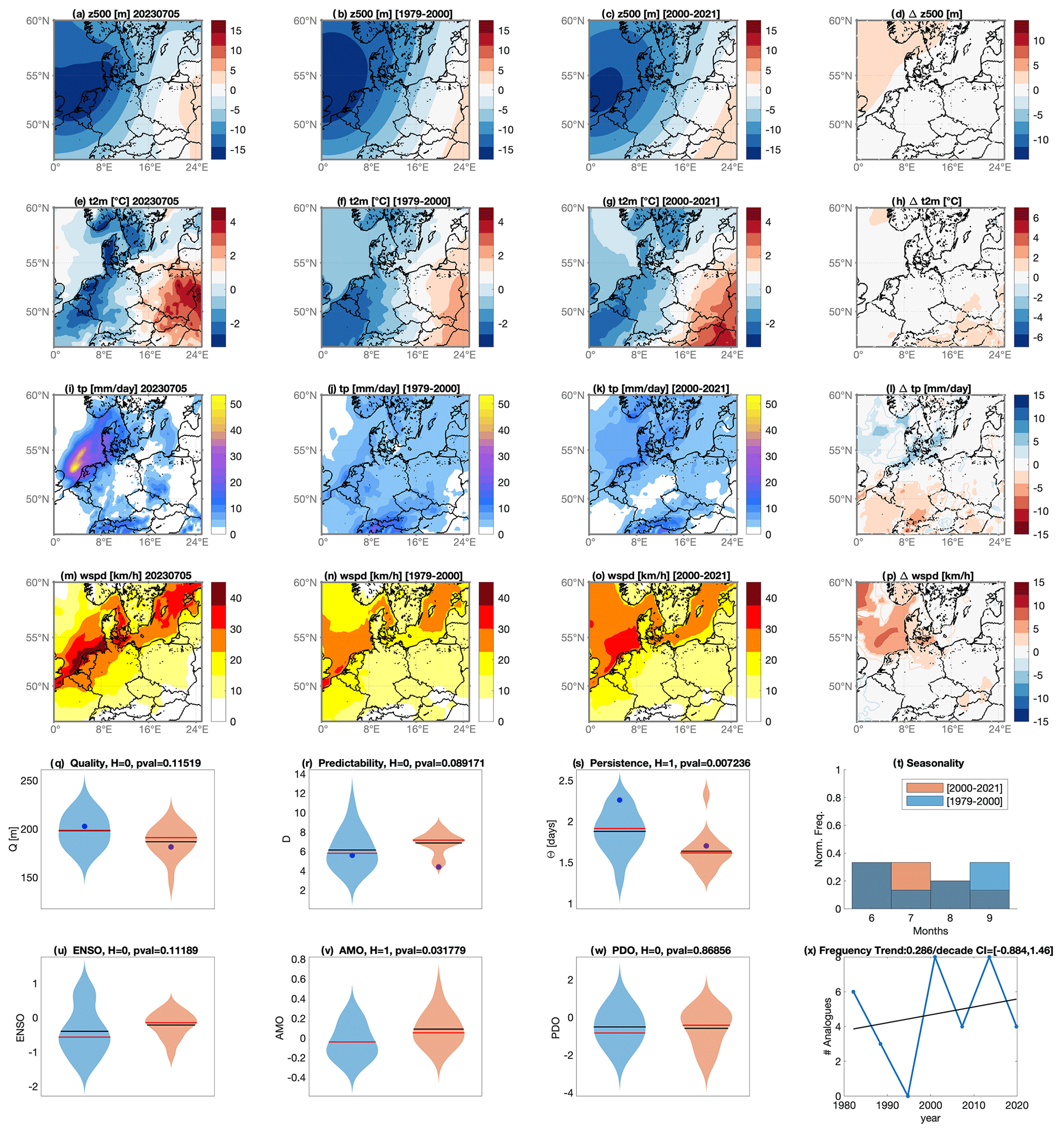
Figure A6 Storm Poly in northern Europe on 5 July 2023. As in Fig. A4 but for ERA5 500 hPa geopotential height (z₅₀₀) data.