Cold air outbreaks drive near-surface baroclinicity variability over storm track entrance regions in the Northern Hemisphere

Cold air outbreaks (CAOs) are key drivers of near-surface baroclinicity in midlatitude oceanic regions, where cold continental air masses interact with warm sea surface temperatures, giving rise to strong surface heat fluxes. Despite their relatively limited spatio-temporal extent, CAOs exert a disproportionate influence on the variability of near-surface baroclinicity, particularly in the entrance regions of the North Atlantic and North Pacific storm tracks. To further clarify this relationship, we use the isentropic slope framework to distinguish between diabatic and adiabatic changes in baroclinicity and quantify the contribution of CAOs to near-surface baroclinicity variability in the Gulf Stream and Kuroshio-Oyashio extension regions.

Moderate-intensity CAOs account for up to 40 % of the total near-surface baroclinicity variability in the Gulf Stream Extension, while occupying less than 15 % of the region. In the Kuroshio-Oyashio Extension, CAOs explain a smaller fraction of variability despite their broader spatial extent. We employ phase space analysis to diagnose the typical phasing between adiabatic depletion and diabatic restoration of baroclinicity, with the former leading in time on the latter. Phase portraits and synoptic composites focused on CAO-related variability show that this characteristic phasing is predominantly linked to CAOs, whereas background variability contributes weakly and incoherently. These findings highlight the central role of CAOs in shaping near-surface baroclinicity and suggest that they are essential to the evolution of midlatitude storm tracks.

1 Introduction

Marine cold air outbreaks (CAOs) are associated with the discharge of cold polar air masses over relatively warm waters, giving rise to intense surface heat fluxes that dominate the total surface heat exchange over polar and subpolar oceans (e.g., Jensen et al., 2011; Isachsen et al., 2013; Harden et al., 2015; Papritz et al., 2015; Papritz and Spengler, 2017). While the occurrence and frequency of CAOs are primarily governed by the large-scale atmospheric flow (Kolstad et al., 2009; Iwasaki et al., 2014; Papritz and Spengler, 2017), the enhancement of temperature gradients during CAOs provides additional baroclinicity variability, potentially feeding back onto the large-scale flow (Charney, 1947; Eady, 1949; Hoskins and Valdes, 1990; Papritz and Spengler, 2015). This two-way interaction is particularly relevant in midlatitude storm tracks, where baroclinicity in the near-surface troposphere is typically depleted adiabatically and subsequently restored diabatically (Marcheggiani and Spengler, 2023). While synoptic features, such as cyclones, fronts, and atmospheric rivers are known to drive baroclinicity variability aloft (Marcheggiani et al., 2025), the specific role of CAOs in modulating near-surface baroclinicity has not been clarified. We complement the upper tropospheric results of Marcheggiani et al. (2025) by quantifying the relative contribution of CAOs to near-surface baroclinicity variability in the entrance regions of the North Atlantic and North Pacific storm tracks.

Beyond their thermodynamic effects, CAOs exert a broader influence on the atmospheric circulation, promoting the formation of polar lows (Terpstra et al., 2016; Michel et al., 2018; Terpstra et al., 2021), moistening air masses that can lead to atmospheric blocking (Wenta et al., 2024), and contributing to the total meridional heat transport (Messori and Czaja, 2013; Pithan et al., 2018). CAOs are most frequent and intense near the sea ice margin and over oceanic western boundary currents, such as the Gulf Stream and the Kuroshio-Oyashio currents (Kolstad et al., 2009; Fletcher et al., 2016). These regions are characterised by strong sea surface temperature (SST) gradients, which amplify the air-sea temperature contrast during CAOs and yield diabatic restoration of near-surface baroclinicity (Nakamura et al., 2008; Sampe et al., 2010; Papritz and Spengler, 2015). However, the extent to which this interaction modulates baroclinicity variability, and thereby storm track dynamics, remains an open question.

To gain a clearer understanding of how CAOs modulate storm track dynamics, one needs to disentangle the mechanisms that drive baroclinicity variability in lower troposphere. While latent heating is the dominant source of diabatic baroclinicity production in the upper troposphere (Papritz and Spengler, 2015; Weijenborg and Spengler, 2020; Marcheggiani and Spengler, 2023), surface sensible heat fluxes play a prominent role in the lower troposphere (Nakamura et al., 2008; Hotta and Nakamura, 2011; Papritz and Spengler, 2015; Marcheggiani and Ambaum, 2020; Marcheggiani and Spengler, 2023). This vertical dichotomy aligns with observed differences in the phasing between adiabatic depletion and diabatic restoration of baroclinicity, whereby diabatic production associated with latent heating typically precedes adiabatic depletion of baroclinicity in the free troposphere (750–350 hPa) (Papritz and Spengler, 2015; Weijenborg and Spengler, 2020; Marcheggiani and Spengler, 2023), while baroclinicity near the surface (900–825 hPa) is restored diabatically following an initial adiabatic depletion, often associated with CAOs (Marcheggiani and Spengler, 2023). Given this dominant role of CAOs, we use the isentropic slope framework (Papritz and Spengler, 2015) to quantify their contribution to near-surface baroclinicity variability and depict the associated synoptic evolution.

2 Data and methods

We use data from the ERA5 reanalysis (Hersbach et al., 2020), interpolated onto a 0.5°×0.5° longitude-latitude grid. We use both 3-hourly instantaneous fields, as well as 6-hourly accumulated temperature tendencies due to parameterisations centred on each 3-hourly time step.

To compute the isentropic slope and its tendencies (Papritz and Spengler, 2015), we use temperature, geopotential height (z), wind velocity ($u,v,w$), and accumulated temperature tendencies due to parameterisations (mttpm) on 24 pressure levels (every 25 hPa between 1000 and 750 hPa, every 50 hPa thereafter up to 100 hPa). Temperature tendencies are only available on model levels and were interpolated to the aforementioned pressure levels.

In the Northern Hemisphere, CAOs are most frequent and intense during the winter months, especially off the sea ice edge and over western sectors of the North Atlantic and North Pacific oceans (Kolstad et al., 2009; Kolstad, 2011; Fletcher et al., 2016). Hence we focus on extended winter months (November to February) from November 1979 to February 2020 over two specific regions previously considered by Marcheggiani and Spengler (2023), namely the Gulf Stream Extension (GSE, 30–60° N, 80–30° W; Fig. 1) and Kuroshio-Oyashio Extension (KOE, 30–50° N, 130–180° E) regions. When calculating spatial averages, we exclude the Sea of Japan from the KOE region, as baroclinicity variability there is not necessarily linked to variability within the main North Pacific storm track (Sect. 2.4 provides a more detailed explanation for this choice). Furthermore, we also exclude grid points covered by land and where sea ice concentration is above 15 % for more than 0.5 % of the time to avoid misrepresentations of surface heat fluxes over sea ice (Renfrew et al., 2021). We apply the resulting mask for all time steps to keep the total area constant.

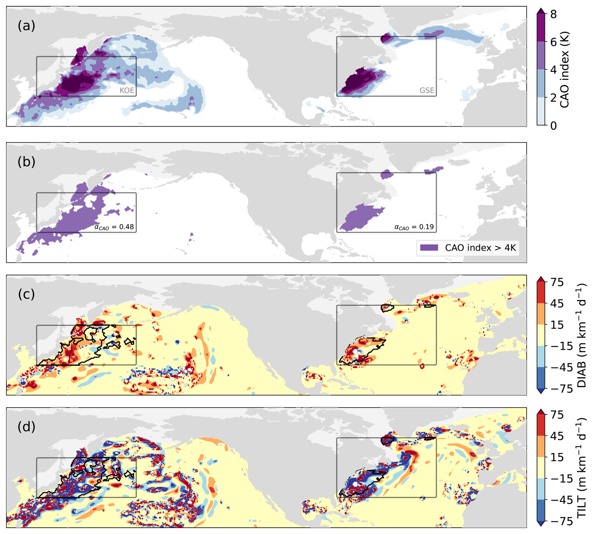
Figure 1 Graphical example of spatial averaging conditioned on CAOs for 23 January 2014 at 15:00 UTC. (a) CAO index (colour shading). (b) Mask M for spatial averaging where the CAO index is above 4 K (grey shading) within the GSE and KOE spatial domains (grey boxes). (c) DIAB, with CAO-only area-mean DIAB indicated by thick black contour. (d) Same as (c) but for TILT. Land grid points, ocean grid points where sea ice concentration is above 15 % for more than 5 % of the time, and grid points pertaining to the Sea of Japan are masked out by grey shading.

2.1 Isentropic slope framework

We use the isentropic slope framework introduced by Papritz and Spengler (2015) to calculate diabatic and adiabatic tendencies in baroclinicity. Baroclinicity is measured as the slope $S\equiv \left|{\mathrm{\nabla }}_{\mathit{\theta }}z\right|$ of isentropic surfaces, where z is altitude and the subscript indicates a horizontal gradient on an isentropic surface. The Eulerian form of the slope tendency equation on pressure levels is

$$\begin{array}{}\text{(1)}& {\displaystyle \frac{\partial S}{\partial t}}{|}_p=\underset{\mathrm{TILT}}{\underbrace{{\displaystyle \frac{{\mathrm{\nabla }}_{\mathit{\theta }}z}{S}}\cdot {\mathrm{\nabla }}_{\mathit{\theta }}{w}_{\text{id}}}}\underset{\mathrm{DIAB}}{\underbrace{-{\displaystyle \frac{\partial z}{\partial \mathit{\theta }}}{\displaystyle \frac{{\mathrm{\nabla }}_{\mathit{\theta }}z}{S}}\cdot {\mathrm{\nabla }}_{\mathit{\theta }}\dot{\mathit{\theta }}}}\underset{\mathrm{ADV}}{\underbrace{-{\displaystyle \frac{\partial S}{\partial \mathit{\theta }}}\mathit{v}\cdot \mathrm{\nabla }\mathit{\theta }}},\end{array}$$

where TILT represents adiabatic tilting by the isentropic displacement vertical wind w_id (Hoskins et al., 2003, their Eq. 8), DIAB describes diabatic deformation due to heating, and ADV accounts for slope advection by the three-dimensional wind $\mathit{v}=(u,v,\mathit{\omega })$. The TILT and DIAB terms generally exert opposing effects on the slope (Papritz and Spengler, 2015; Marcheggiani and Spengler, 2023). The ADV term is generally weaker, although its magnitude becomes comparable to the other two terms near the surface (Papritz and Spengler, 2015; Marcheggiani and Spengler, 2023). In the context of CAOs, ADV tends to strengthen as cold air masses move over the GSE and KOE regions (not shown). While ADV represents the advection of isentropic slope by the atmospheric flow, and thus implicitly captures adiabatic changes in slope, its physical interpretation is less straightforward, as it is not directly linked to a specific mechanism that modifies isentropic surfaces. For this reason, we chose to exclude ADV from our analysis and instead focus on the TILT term, which has a clearer physical meaning as the kinematic flattening of isentropic surfaces through baroclinic rearrangement of mass.

As in Marcheggiani et al. (2025), data are first spatially filtered by spectral truncation to T84 to filter out small-scale features (e.g., gravity waves) that can be associated with extremely steep slopes that are not relevant to study larger scale baroclinic development. Furthermore, we follow Papritz and Spengler (2015) to avoid any numerical issues related to extremely steep isentropic slopes by masking out any grid point where the static stability $\partial \mathit{\theta }/\partial z<{\mathrm{10}}^{-\mathrm{4}}$ K m⁻¹. We focus on the near-surface troposphere and thus consider vertical averages of slope, TILT, and DIAB between 900 and 825 hPa (consistent with Marcheggiani and Spengler, 2023). ERA5 is considered sufficiently reliable for this layer, as supported by previous studies (Seethala et al., 2021; Lavers et al., 2020; Simmons, 2022), which show only minor biases mostly below 900 hPa and outside our focus region.

2.2 Detection of Cold Air Outbreaks

To detect CAOs we follow (Papritz et al., 2015) and first calculate the CAO index, defined as air-sea potential temperature difference,

$$\begin{array}{}\text{(2)}& \text{CAO index}={\mathit{\theta }}_{\text{SST}}-{\mathit{\theta }}_{\mathrm{850}},\end{array}$$

where θ_SST is potential sea surface temperature and θ₈₅₀ is potential temperature at 850 hPa. CAOs are detected over those ocean grid points where the CAO index exceeds a certain threshold, θ_T. Different thresholds will result in the detection of CAOs of different intensity, with moderate intensity and stronger mostly captured by using θ_T=4K (Papritz et al., 2015; Papritz, 2017; Papritz and Spengler, 2017). This method based on the CAO index likely captures more than just canonical CAOs, particularly when using thresholds below 4 K. Such lower thresholds tend to encompass broader regions in the North Pacific compared to the North Atlantic (Fig. 1a), so the CAO-index may capture more than CAOs in the North Pacific (e.g., cold sectors of extra-tropical cyclones). Nonetheless, the 4 K threshold is widely used to identify CAOs and, from a thermodynamic perspective, should still reflect similarly strong air–sea interactions characteristic of these events. We also point out that we do not exclude stronger CAOs by lowering the threshold; rather, we expand the extent of area covered to include both weak and more intense events.

2.3 Partitioning contributions from CAOs to baroclinicity variability

We study the temporal variability associated with the evolution of the North Atlantic and North Pacific storm tracks by considering spatial averages of slope, DIAB, and TILT (Eq. 1) over the GSE and KOE regions. Total variability is partitioned into CAO and non-CAO contributions following a similar approach to Marcheggiani et al. (2025). We first construct a CAO mask M based on the CAO index,

$$\begin{array}{}\text{(3)}& M_i\left(t\right)=M({\text{lon}}_i,{\text{lat}}_i;t)=\left\{\begin{array}{ll}\mathrm{1}& \text{if }\text{CAO index}\ge {\mathit{\theta }}_{\mathrm{T}}\\ \mathrm{0}& \text{otherwise},\end{array}\right.\end{array}$$

which is then used to construct time series of CAO area mean,

$$\begin{array}{}\text{(4)}& {\mathit{\chi }}_{\text{CAO}}\left(t\right)={\displaystyle \frac{{\sum }_i{a}_i{M}_i\left(t\right){\mathit{\chi }}_i\left(t\right)}{{\sum }_i{a}_i{M}_i\left(t\right)}},\end{array}$$

and background, non-CAO area mean,

$$\begin{array}{}\text{(5)}& {\mathit{\chi }}_{\text{noCAO}}\left(t\right)={\displaystyle \frac{{\sum }_i{a}_i[\mathrm{1}-M_i(t\left)\right]{\mathit{\chi }}_i\left(t\right)}{{\sum }_i{a}_i[\mathrm{1}-M_i(t\left)\right]}}.\end{array}$$

Sums in Eqs. (4)–(5) are over all grid points in the averaging box. The areal extent of each grid point is represented by a_i, while χ_i represents the value of either slope, DIAB, or TILT at that grid point.

At each time step, CAOs occupy a fraction of the total area,

$$\begin{array}{}\text{(6)}& {\mathit{\alpha }}_{\text{CAO}}\left(t\right)={\displaystyle \frac{{\sum }_i{a}_i{M}_i\left(t\right)}{{\sum }_i{a}_i}}.\end{array}$$

By construction, the time series of the total area mean is the sum of the CAO component (Eq. 4) and non-CAO, background component (Eq. 5) weighted by the area fraction (Eq. 6) occupied by CAOs,

$$\begin{array}{}\text{(7)}& {\mathit{\chi }}_{\text{tot}}={\displaystyle \frac{{\sum }_i{a}_i{\mathit{\chi }}_i\left(t\right)}{{\sum }_i{a}_i}}=\mathit{\alpha }{\mathit{\chi }}_{\text{CAO}}+(\mathrm{1}-\mathit{\alpha }){\mathit{\chi }}_{\text{noCAO}}.\end{array}$$

An example of the partition in CAO and background components is presented in Fig. 1. The CAO index is significantly larger than zero over large areas both in the North Atlantic and especially in the North Pacific oceans (Fig. 1a). Then we only consider CAOs of at least moderate intensity by choosing θ_T=4K and obtain the corresponding mask M (Fig. 1b). Finally, we look at χ= DIAB and χ=TILT, and calculate DIAB_CAO and TILT_CAO as the area-mean over those grid points within the averaging domain that also belong to the mask, that is both inside the grey boxes and within the thick black contour (Fig. 1c, d). In this case, the CAO in the KOE region extends over almost half the domain (α_CAO=0.48), while only covering about a fifth in the GSE region (α_CAO=0.19).

2.4 Constructing the DIAB-TILT phase space

Using time series for area-mean DIAB and TILT defined in either Eqs. (4), (5), or (7), we construct phase portraits for CAO, background, and total variability, respectively. Similar to Marcheggiani and Spengler (2023), we utilise a Gaussian kernel with averaging length scale equal to half of the standard deviation in either of the time series. We then define a stream function ψ (black contours in Fig. 3) to visualise the non-divergent flow in the phase space, so that

$$\begin{array}{}\text{(8)}& \mathbf{F}=(\mathit{\varrho }{c}_x,\mathit{\varrho }{c}_y)=(-{\displaystyle \frac{\mathrm{d}\mathit{\psi }}{\mathrm{d}y}},{\displaystyle \frac{\mathrm{d}\mathit{\psi }}{\mathrm{d}x}}),\end{array}$$

where F=ϱc is the mass flux, ϱ is the data density at each point in the phase space, and $\mathit{c}=(c_x,c_y)$ represents the phase space velocity field. We can also estimate typical values of various variables, whether one-dimensional, like the area-mean slope (illustrated by the shading in Fig. 3), or two-dimensional, such as geopotential, shown for a specific point in the phase space in Fig. 4. Specifically, these average values are also obtained using a kernel-weighted method: each value is multiplied by a weight based on its distance from the phase space grid point, and the result is then divided by the estimated local density. This yields the kernel-averaged value of the variable at each location in the phase space. We refer the reader to Novak et al. (2017) and Marcheggiani et al. (2022) for more technical details on the construction of the phase portraits.

The decision to exclude the Sea of Japan from spatial averaging in the North Pacific storm track was guided by phase space analysis. When examining the Sea of Japan in isolation, we observed a circulation pattern in phase space (not shown) similar to those seen in the GSE and KOE regions, characterised by anticlockwise oscillations in the negative-TILT, positive-DIAB quadrant. These oscillations tend to have larger amplitudes for the Sea of Japan, likely due to the smaller size of the averaging domain. However, the variability in the Sea of Japan does not appear to be coherent with that of the Kuroshio-Oyashio Extension, as the associated phase portrait for the combination of both regions is noticeably noisier (not shown). Hence we chose to exclude the Sea of Japan from our selected spatial domain in the North Pacific to focus more precisely on the primary storm track entrance region.

3 Quantifying CAO contribution to total baroclinicity variability

The strongest DIAB and TILT are generally collocated with the largest values of the CAO index (compare Fig. 1a and c, d). The fraction of total variance explained by CAOs can be determined by the covariance between the total and the CAO time series, normalised by the total variance,

$$\begin{array}{}\text{(9)}& R_{\text{CAO}}={\displaystyle \frac{\mathrm{Cov}({\mathit{\chi }}_{\text{tot}},{\mathit{\chi }}_{\text{CAO}})}{\mathrm{Var}\left({\mathit{\chi }}_{\text{tot}}\right)}},\end{array}$$

where a high degree of similarity between two time series results in a ratio approaching one, suggesting that the variability in one time series significantly contributes to the variability in the other. Conversely, if the two time series are largely uncorrelated, or have significantly different variances, the ratio remains near zero, indicating a minimal contribution of the variability in one time series to the other.

We assess the contribution of CAOs to total variability relative to their intensity as measured by the CAO index (Eq. 3). Using larger CAO index thresholds (θ_T in Eq. 3) yields smaller CAO masks, evident from the decreasing area fractions in Fig. 2 with increasing CAO index threshold.

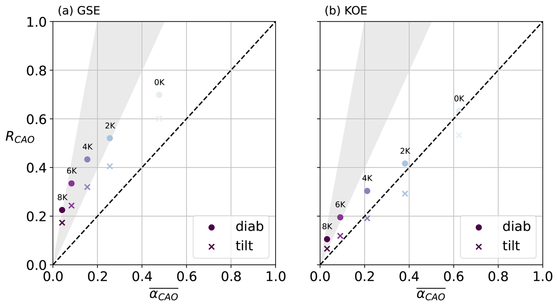
Figure 2 Fraction R_CAO (Eq. 9) of DIAB (dots) and TILT (crosses) plotted against the mean area fraction occupied by $\stackrel{\mathrm{‾}}{{\mathit{\alpha }}_{\mathrm{CAO}}}$. Markers are colour-coded according to the CAO index threshold (Eq. 3), with corresponding values annotated. The dashed line indicates the 1–1 line, while the grey shaded area highlights the sector where the ratio between R_CAO and mean $\stackrel{\mathrm{‾}}{{\mathit{\alpha }}_{\mathrm{CAO}}}$ is in the range 2:1–3:1.

Over the GSE region, moderate and strong CAOs (CAO index ≥4 K, Fig. 2) contribute disproportionately to the total variance compared to their areal extent, with the strongest CAOs (CAO index ≥8 K) extending over a minimal fraction of the domain (α_CAO≈0.04) while explaining up to 5 times the total variance (R_CAO≈0.2). Thus CAOs explain almost half (40 %–45 %) of the total variance in baroclinicity in the GSE despite only extending over less than 20 % of region. Including weaker CAOs (CAO index ≥2 K or ≥0 K), the areal extent increases significantly (25 %–50 % of the domain) while the associated baroclinicity variability explains up to 70 % of the total variance. CAOs explain less variance in TILT compared to DIAB. This is consistent with TILT being more noisy than DIAB (Fig. 1c, d), therefore more variability occurs in the entire averaging domain, also outside of CAO masks.

Over the KOE region, CAOs typically extend over larger areas compared to their counterparts in the GSE. This is evident in the example in Fig. 1, where positive CAO-indices extend significantly farther south- and eastwards, away from the Asian continent. The larger extent of identified CAOs over the KOE region can be ascribed in part to the East Asian winter monsoon (Zhang et al., 1997; Compo et al., 1999), leading to a stronger cold air mass stream over the North Pacific compared to the North Atlantic (Iwasaki et al., 2014). Similar CAO index thresholds may detect quite different synoptic events across the two basins, so that the CAO mask used in the North Pacific may actually encompass more than CAOs, including unrelated variability. We therefore speculate that the observed differences between the two ocean basins may stem from the distinct characteristics of CAOs in each region.

Moderate CAOs (CAO index ≥4 K) extend over more than 20 % of the KOE, compared to about 15 % for GSE (Fig. 2b). Although stronger CAOs (CAO index ≥6 K) have comparable spatial extent in both regions (${\stackrel{\mathrm{‾}}{\mathit{\alpha }}}_{\text{CAO}}\approx \mathrm{0.08}$ in the KOE, ${\stackrel{\mathrm{‾}}{\mathit{\alpha }}}_{\text{CAO}}\approx \mathrm{0.09}$ in the GSE), they account for a smaller share of the total variance in both TILT and DIAB in the KOE (R_CAO≈0.12–0.20) compared to the GSE (R_CAO≈0.23–0.33). Thus, despite occupying slightly more than 20 % of the area, CAOs in the KOE explain only 20 %–30 % of the total variance.

The strongest CAOs (CAO index ≥8 K) in the KOE account for two to three times more of the total DIAB variance than their spatial extent would imply (Fig. 2b). In contrast, TILT variance increases proportionally with the area fraction as the CAO index threshold is relaxed, indicating that its variability is not strongly linked to CAOs, especially in the KOE. For other CAO categories, the explained DIAB variance generally scales with the areal extent of CAOs, while moderate and weak CAOs (CAO index ≤4 K) account for even less of the total variance in TILT than their areal extent (Fig. 2b). Overall, CAOs in the KOE region thus play a different role in the evolution of near-surface baroclinicity compared to the GSE region despite their similar intensity.

4 CAO-based phase portraits

To assess the coherence of variability explained by CAOs with the total variability, we focus on CAOs of moderate and stronger intensity (CAO index ≥4 K; Papritz and Spengler, 2017) and construct phase portraits of DIAB and TILT for the total (DIAB_tot, TILT_tot, Fig. 3a, d), CAO (DIAB_CAO, TILT_CAO, Fig. 3b, e), and background (DIAB_noCAO, TILT_noCAO, Fig. 3c, f) time series.

Figure 3 Phase portraits of DIAB (x-coordinate) and TILT (y-coordinate) constructed using total (a, d), CAO (b, e), and background (c, f) time series for the GSE (a–c) and KOE (d–f) regions. Kernel-averaged mean-slope is shown in shading, offset and scaled according to the mean and standard deviations of the slope time series, respectively, annotated in the upper right corner of each panel. Contours represent the stream function associated with the kernel-averaged phase space circulation. Points where data is scarce (less than 0.5 % of maximum data density) are blanked out. The size of the Gaussian filter used to construct the phase portrait is indicated by the black-shaded dot in the lower-left corner. Star markers indicate locations in the phase space where the kernel composites are evaluated (see Fig. 4).

Phase portraits based on total variability for the GSE (Fig. 3a) and KOE (Fig. 3d) regions are qualitatively similar. The primary circulation is in the anticlockwise direction, indicating that TILT leads in time over DIAB. While the choice of a starting point is arbitrary, it is most natural to start from the point of weakest DIAB and TILT. Thus, baroclinicity is first adiabatically depleted by tilting and subsequently restored diabatically, consistent with Marcheggiani and Spengler (2023). For both regions, the steepest slope coincides with strongest DIAB and TILT, while the mean slope is larger over the KOE (4.2 m km⁻¹) compared to the GSE (3.4 m km⁻¹). The amplitude of the oscillations reaches up to 30 m km⁻¹ d⁻¹ in both regions, though the phase space flow for the KOE region is somewhat noisier, featuring a secondary clockwise circulation when TILT exceeds −30 m km⁻¹ d⁻¹ (Fig. 3d).

Phase portraits based on CAO variability (Fig. 3b, e) are qualitatively identical to the ones for the total variability (Fig. 3a, d). In both the GSE and KOE regions, the primary circulation in the phase space is also anticlockwise, indicating that the lead in time of TILT over DIAB is strongly linked with CAO-related variability. The magnitude of oscillations in the CAO phase portraits is comparable to those in total variability phase portraits, with values of DIAB reaching up to 20 m km⁻¹ d⁻¹, just slightly weaker than for the total variability (up to 25–30 m km⁻¹ d⁻¹).The secondary clockwise circulation in the KOE region is reproduced for the CAO time series, suggesting it is also linked to CAO dynamics. This secondary circulation is associated with particularly strong values of TILT and reflects a genuine mean behaviour in the DIAB–TILT relationship in the KOE. We suspect that the extreme values of TILT are the result of a deep boundary layer extending into the near-surface troposphere, as suggested by composites of mean boundary layer height (not shown). Although we apply a mask for extreme slope and slope tendencies, large values may still persist near these masked grid points, especially within CAOs, whose phase portrait feature an even stronger secondary circulation (Fig. 3e). Upon examining the synoptic conditions associated with these secondary circulations (not shown), however, we do not find any consistent or recurring patterns that would suggest an underlying physical mechanism explaining such behaviour in the phase space.

In the background, on the other hand, the typical evolution of DIAB and TILT is significantly different. For GSE, DIAB leads in time over TILT, evident by the clockwise direction of the main phase space circulation (Fig. 3c), which actually resembles the typical evolution observed in the free troposphere (Marcheggiani and Spengler, 2023). The circulation is also noisier, as secondary ripples depart from the main circulation. Furthermore, the amplitude of the oscillations is weaker than that for the total and CAO phase space.

The background-based phase portrait for the KOE region exhibits an even higher degree of noise, making it difficult to identify any clear or consistent circulation pattern (Fig. 3f). Instead, the phase portrait is characterised by numerous smaller-scale circulation cells that appear scattered and disorganised. The noise observed in Fig. 3f suggests the absence of a single dominant physical mechanism governing the co-variability of DIAB and TILT outside of cold air outbreaks in the KOE region. We speculate that the processes driving this variability are poorly organized in both space and time, making it particularly difficult to capture a coherent signal in synoptic composites, where any underlying structure may be lost during the averaging process.

5 Synoptic perspective

To gain further mechanistic insights, we present the synoptic conditions associated with the strongest TILT along the primary circulation within the total, CAO, and background phase portraits. The background phase portrait for the KOE region is particularly noisy and there is no clear circulation, so we select a point with similar proportions between the magnitudes of TILT and DIAB as in the other phase portraits. The specific location of these points in each phase portrait is marked in Fig. 3.

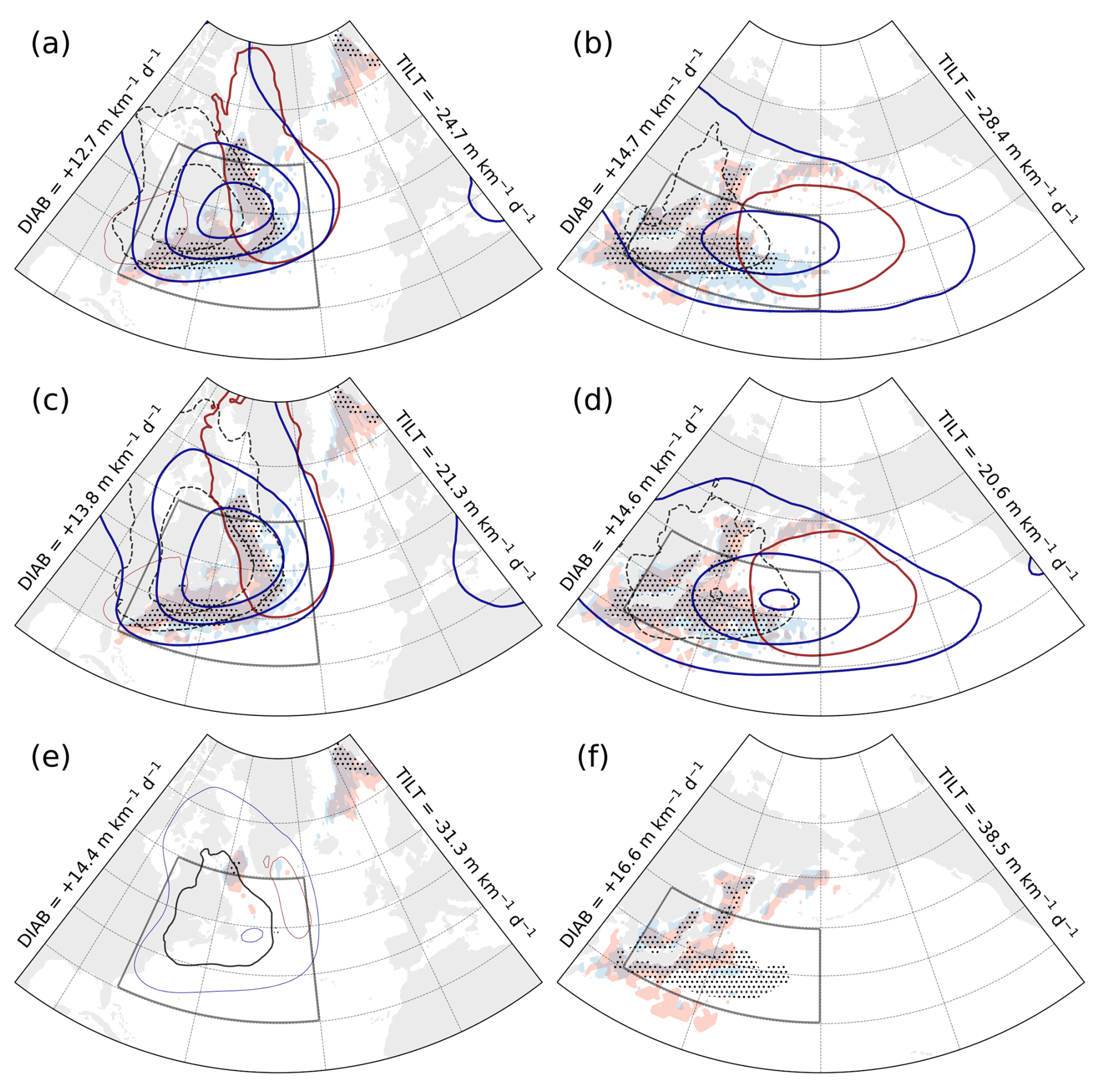
Figure 4 (a, c, e) GSE and (b, d, f) KOE phase composite for (a, b) total, (c, d) CAO, and (e, f) non-CAO phase portraits (Fig. 3). Contours of Z1000 and Z500 (red and blue, respectively) represent the anomaly field relative to climatology (NDJF, 1979–2020) and are plotted every 4 dam (0 dam contours omitted; thin and thick solid lines represent positive and negative contours, respectively). Ratio of TCWV to climatology is shown in black contours (±15 % and ±30 %, negative values dashed). Grid points were CAO occurrence is above 40 % are stippled. Shading for DIAB (red) and TILT (blue) indicates values above 15 m km⁻¹ d⁻¹ for DIAB, below −15 m km⁻¹ d⁻¹ for TILT. Area-mean values of DIAB and TILT are annotated outside of each panel.

Phase composites based on the total variability time series for the GSE (Fig. 4a) and KOE (Fig. 4b) regions feature negative, cyclonic geopotential anomalies both at the surface and in the free troposphere. Free tropospheric anomalies are shifted westwards compared to surface anomalies, suggesting baroclinic development. This configuration is also conducive to advection of cold air masses from the North American (Fig. 4a) or the East Asian (Fig. 4a, b) continents, respectively, which is reminiscent of the typical onset of CAOs in these regions (Kolstad et al., 2009; Fletcher et al., 2016).

The anomalous moisture distribution is also consistent with advection of drier continental air masses over the western North Atlantic and North Pacific oceans, as total column water vapour (TCWV) is up to 15 % and 30 % lower than climatology over the East Asian and North American continents, respectively. Additionally, regions of strong TILT extend farther east over both the North Atlantic and North Pacific than regions of strong DIAB.

Composites at different, adjacent points in the phase space (not shown) reveal that peaks in both DIAB and TILT propagate eastward over the ocean. The fact that TILT peaks further downstream than DIAB is consistent with TILT leading in time over DIAB observed in the phase portraits (Fig. 3a, d).

Phase composites based on CAO time series (Fig. 4c, d) are qualitatively identical to those based on total variability in both the GSE (compare Fig. 4a, c) and KOE (compare Fig. 4b, d) regions. Negative geopotential anomalies are slightly stronger than in the total variability composites. Similarly, the dry signal from cold continental air masses is amplified, as areas of 15 %–30 % lower TCWV expand farther inland over North America (Fig. 4c) and East Asia (Fig. 4d). The distribution of CAO occurrence is also qualitatively unchanged between total and CAO phase composites, reflecting the fact that CAOs are the primary contributors to total variability in both regions.

A significantly different picture emerges from background composites for both GSE and KOE (Fig. 4e, f), where the signal almost disappears. The sign of the geopotential height and TCWV anomalies is actually opposite, indicating weakly anticyclonic flow and slightly higher moisture content (up to 15 % more than climatology). Over the North Atlantic (Fig. 4e), both DIAB and TILT are substantially weaker, as is the frequency of CAOs. In contrast, the KOE background composite still shows relatively strong DIAB, especially near the western North Pacific coast, along with a comparatively high frequency of CAOs.

The persistence of CAOs, even in the background composite, reflects the climatologically frequent occurrence of CAOs and stronger DIAB in KOE, reaching up to 60 % of all winter days (not shown). The higher CAO frequency in the KOE is likely driven by the combined influence of the East Asian winter monsoon (Zhang et al., 1997) and the East Asian cold air stream (Compo et al., 1999; Iwasaki et al., 2014), both of which favour frequent and extended cold surges. Consequently, the relatively high CAO occurrence is partially retained when compositing.

6 Conclusions

Cold air outbreaks (CAOs) are a recurrent synoptic feature in the North Atlantic and North Pacific storm track entrance regions. The strong surface heat fluxes associated with CAOs exert a significant influence on the variability of near-surface baroclinicity by anchoring midlatitude storm tracks to the strong SST gradients associated with western boundary currents. To clarify the role of CAOs in near-surface baroclinicity, we isolated diabatic and adiabatic changes in baroclinicity by using the isentropic slope framework (Papritz and Spengler, 2015), and quantified the contribution of CAOs to the total baroclinicity variability in the near-surface troposphere (900–825 hPa), where baroclinicity is diabatically restored following an initial adiabatic depletion typically associated with the advection of cold air masses (Marcheggiani and Spengler, 2023). While cyclones and fronts constitute the main contributors to the total variability of free-tropospheric baroclinicity (Marcheggiani et al., 2025), our results highlight the distinct and complementary role of CAOs in driving baroclinicity variability in the lower troposphere.

Despite their relatively small area, CAOs account for most of the total variability in near-surface baroclinicity. In the North Atlantic, CAOs of moderate intensity (CAO index above 4 K, see Eq. 2) account for around 40 % of the total variability in near-surface baroclinicity while extending over less than 15 % of the Gulf Stream Extension (GSE) region (Fig. 2a). In the North Pacific, the contribution from CAOs to total variability is less clear, as they are found to explain less than 30 % of the total variability despite occupying, on average, more than 20 % of the Kuroshio-Oyashio Extension (KOE) region (Fig. 2b). The larger areal extent compared to CAOs in the North Atlantic is likely due to the combined effect of the East Asian winter monsoon and East Asian cold air stream (Zhang et al., 1997; Iwasaki et al., 2014), which allows for cold continental air masses associated with CAOs to reach further south-west into the Pacific Ocean compared to CAOs in the North Atlantic.

Most of the adiabatic depletion through tilting of isentropic surfaces (TILT) and diabatic restoration (DIAB) of near-surface baroclinicity takes place within CAOs. The particular phasing between TILT and DIAB, with TILT leading in time on DIAB, is also primarily associated with CAOs. This is evidenced by phase portraits based on CAO-related baroclinicity variability (Fig. 3b, e), which are qualitatively identical to those based on total variability (Fig. 3a, d) and consistent with previous results by Marcheggiani and Spengler (2023). The signature of CAOs is also evident from composites based on strong TILT and DIAB, where the synoptic conditions emerging from both total (Fig. 4a, b) and CAO (Fig. 4c, d) variability feature cyclonic flow over both GSE and KOE region, advecting cold, dry air off the North American and Northwestern Asian continents over the adjacent ocean basins.

Background, non-CAO based phase portraits (Fig. 3c, f), on the other hand, are significantly different. In the GSE region, the phasing between background DIAB and TILT is reversed and actually more similar to what is observed in the free troposphere (see Marcheggiani and Spengler, 2023, their Fig. 3). The limited influence of background variability on the total variability provides further evidence to the importance of CAOs in explaining the lower-upper troposphere dichotomy in the maintenance of baroclinicity. Compared to CAO-based composites, the signal emerging from composites of strong background TILT and DIAB (Fig. 4e, f) is significantly weaker and of opposite sign, as only weak anticyclonic and dry anomalies are detected.

The background-based phase space circulation in the KOE (Fig. 3f) is largely incoherent and affected by a higher degree of noise compared to the GSE. This points to the lack of a clear phasing between DIAB and TILT variability in the KOE background (i.e., outside of CAOs). This is partly explained by the more frequent and deeper south-westward extension of CAOs in the KOE region compared to CAOs in the GSE, as evidenced by the relatively high occurrence of CAOs in the KOE, even when excluding CAOs (Fig. 4f). Since moderate-intensity CAOs appear to develop continuously over the KOE, background variability becomes marginal. CAOs in the KOE thus play a more dominant role in shaping near-surface baroclinicity variability than in the GSE.

Given their central role in restoring near-surface baroclinicity, our results indicate that CAOs should be considered an integral part of the life cycle of midlatitude storm tracks. Recognising the role of CAOs in restoring near-surface baroclinicity not only highlights their contribution to storm track maintenance, but also underscores their relevance for advancing our theoretical understanding of how diabatic processes near the surface shape storm track evolution and their interaction with oceanic boundary currents.