The impact of synoptic meteorology on observed surface heat fluxes over the Southern Ocean

A 14-year climatology of the bulk sensible and latent heat fluxes (SHF and LHF) made from the Southern Ocean Flux Station (SOFS) is analysed with respect to the synoptic meteorology and mesoscale cellular convection (MCC). A K-means clustering algorithm identified five synoptic regimes: High Pressure/Ridging (HPR), Tasman Blocking High (TBH), Zonal, Frontal, and Cold Air Advection (CAA). Among these, the CAA regime exhibited the most pronounced air-sea coupling, with a mean SHF of −40.4 W m⁻² and LHF of −131.0 W m⁻², which are 3.5 and 2 times greater than the overall mean, respectively. For the Zonal, Frontal, and CAA regimes, a strong correlation between the surface fluxes and the M-index (surface − 850 hPa potential temperature difference) is observed, with an R² of 0.58 for the SHF and M-index relationship in the Zonal regime and an R² of 0.48 for the LHF and M-index in the CAA regime when the estimated inversion strength (EIS) is less than zero. Furthermore, the flux transfer rate demonstrates a two-fold increase with the M-index when the capping inversion weakens and collapses (EIS shifts from > 0 to < 0). The relationship between surface fluxes and the M-index is weak in the HPR and TBH regimes, which are characterised by stronger inversions at SOFS. Turning to open and closed MCC, relatively smaller differences in the fluxes are observed between these two cloud states at SOFS, indicating that SHF and LHF are not the primary drivers in the transition between these cloud types. However, the EIS and M-index exhibit considerable differences between the cloud types, which may be more significant for the morphology of open and closed MCCs, rather than the surface flux release. The SOFS measurements were employed to evaluate ERA5 fluxes, revealing that ERA5 accurately represents the observed bulk SHF and LHF with significant correlation coefficients of r = 0.9 (p < 0.01) and 0.92 (p < 0.01), respectively. A mean bias of 1.6 W m⁻² is noted for SHF and −6.2 W m⁻² for LHF in ERA5. The bias in SHF is attributed to the underestimation of wind speed (10 m) in ERA5, whereas the dry bias of specific humidity (2 m) leads to the overestimation of LHF.

1 Introduction

The Southern Ocean (SO) is responsible for about 75 ± 22 % of the excess heat absorbed by the world's oceans each year, moderating global temperatures (Frolicher et al., 2015; Williams et al., 2024). Sea surface temperature (SST) variability and heat uptake into the SO profoundly impact climate change and global circulation, which may substantially influence remote tropical climate systems in the coming decades (Jeong et al., 2025). Although the SO influences the global climate, many climate models have consistently shown a notable radiative bias over the SO for several generations (Trenberth and Fasullo, 2010; Schuddeboom and McDonald, 2021). The radiative bias in the Coupled Model Intercomparison Project (CMIP) phase 5 and 6 over the SO has been attributed to errors in depicting cloud fraction and phase (Zelinka et al., 2020; McFarquhar et al., 2021) and resulting substantial warm biases in SO SST (Sallée et al., 2013; Meijers, 2014).

Accurate surface flux estimates are essential for determining the energy budget, as they shape the mixed layer temperature, SST, heat content, and ocean circulation (Niiler and Kraus, 1977; Yu et al., 2006; Schott et al., 2009). While many advances have been made in assessing surface fluxes, achieving closure of energy and water budgets at the air-sea interface over the SO remains a challenge, primarily due to limited direct measurements (Bharti et al., 2019). Valdivieso et al. (2017) documented that the Ocean Reanalysis Intercomparison Project (ORA-IP) ensemble, comprising 16 flux estimates, exhibits a global average positive bias in net heat gain of 4.2 ± 1.1 W m⁻² for the period from 1993 to 2009 (Valdivieso et al., 2017). The study further observed that the variability among these products increases markedly in the SO, while it remains relatively stable in the northern subtropical and higher latitudes. Previous studies have reported significant uncertainty in the net surface heat flux products over the global oceans (Large and Yeager, 2009; Mayer et al., 2022).

ERA5 is the most recent global reanalysis output from the European Centre for Medium-Range Weather Forecasts (ECMWF), which utilises data simulation systems based on coupled numerical models to assimilate multiple fields gathered from surface observations and remote sensing techniques (Hersbach et al., 2020). Pokhrel et al. (2020) showed that over the tropical Indian Ocean, ERA5 flux performs best among all other reanalysis products with buoy observation, with correlations of 0.89 for net flux, 0.71 for sensible heat flux (SHF) and 0.90 for latent heat flux (LHF). At the same time, studies have noted significant mean state differences in surface net heat flux of up to 50 W m⁻² between reanalysis products, including ERA5, over vast swaths of the SO (Swart et al., 2019). This indicates the performance of ERA5 is not uniform; it can vary significantly across regions and seasons (Gossart et al., 2019), and the errors are particularly notable in data-sparse regions such as the SO (Rowe et al., 2025; Hobbs et al., 2020). The uncertainties stemming from observation errors, spatial and temporal heterogeneity of data sources, and intrinsic uncertainties within numerical models often accompany reanalysis estimates (Bosilovich et al., 2008; Liu et al., 2011). Sivam et al. (2024) reported that the SHF and LHF from ERA5 effectively represent the mean characteristics of air-sea exchanges in the sub-Arctic region. However, they noted that the errors in ERA5 fluxes increase when examining high-frequency variability, such as synoptic weather events. The international climate research community aims to measure each element of the surface heat budget with a high degree of precision, targeting a range of within 5 W m⁻², alongside spatial and temporal resolutions of 1° and 3–6 h, respectively (Curry et al., 2004). To reach this objective, it is necessary to establish an adequate number of direct flux measurement stations in remote areas such as the SO. The Southern Ocean Flux Station (SOFS), located at 47° S, 142° E, was established under the auspices of the Australian Integrated Marine Observing System (IMOS) (Hill et al., 2010; Schulz et al., 2012), is regarded as the benchmark for the measurement of flux data over the high latitudes of the SO, and the measurements made by the maintained surface moorings have proven to be of high value (Josey et al., 2023).

Across the SO, an increase in the heat flux from the ocean to the atmosphere can intensify extratropical storms (Yau and Jean, 1989; Kuwano-Yoshida and Minobe, 2017) and alter the stability of both the ocean and atmosphere (Neiman et al., 1990; Chen et al., 2010). Earlier research has indicated a potential link between mesoscale SST anomalies and synoptic storms (Small et al., 2008; Su et al., 2018), feeding back on the air-sea fluxes. Surface heat fluxes play a vital role in cyclogenesis (Yokoyama and Yamamoto, 2019), but the stage of cyclonic development may also affect flux variability. Using data from the Clouds Aerosols Precipitation Radiation and atmospheric Composition over the Southern Ocean (CAPRICORN) experiment, Bharti et al. (2019) observed a notable decrease in heat fluxes within the warm sector of storms over the SO, with significant variations in SHF ranging from −91 to 103 W m⁻² and LHF from −105 to 180 W m⁻². Similarly, Shao and Wu (2024) noted that frontal passage weakens the influence of SST gradients on surface wind divergence SO, leading to a significant decline in coupling compared to the days immediately preceding and following these events. The greatest variability in air-sea flux magnitude over the SO occurs during winter, marked by synoptic-scale cold air outbreaks, where cold, dry air moves over warmer water, leading to episodic high flux events (Shaman et al., 2010). Despite these findings, a notable gap remains in the literature related to the influence of different synoptic regimes on air-sea interactions over the SO, particularly based on long-term observational data.

At 47° S, the synoptic meteorology of the SOFS station is primarily defined by the nearby SO storm track (Truong et al., 2020) with the rapidly evolving weather patterns defining the structure of the marine atmospheric boundary layer (MABL) clouds (McCoy et al., 2017; Naud et al., 2016). Wood and Hartmann (2006) categorized four basic structures for MABL clouds: open mesoscale cellular convection (MCC), closed MCC, no MCC, and disorganized cellular clouds. Wood et al. (2011) documented that cloud-base precipitation rates are similar in both open and closed overcast areas. However, they noted that over 90 % of precipitation evaporates below the cloud in the closed region due to a smaller droplet size resulting from a larger number (∼ 100 cm⁻³) of accumulation mode aerosol particles. At the same time, substantial surface precipitation occurs within the open cell, characterised by low aerosol concentrations (∼ 30 cm⁻³) and efficient coalescence scavenging and sedimentation processes. The surface fluxes and boundary layer stability regulate the initiation, depth, and persistence of boundary-layer clouds (Wood, 2012; Su et al., 2023), as they control buoyancy production and moisture supply from the surface. However, the relationship between fluxes and stability indices for open and closed MCCs is limited in the literature, and there has been no validation of ERA5 flux during open and closed MCC periods.

Using 14 years of observations from the SOFS, this study examines the variability in SHF and LHF over the SO during different synoptic weather regimes and their relationships with the thermodynamic structure of the MABL, as defined by the M-index and the estimated inversion strength (EIS). The modulations in SHF and LHF during open and closed MCC periods are also investigated, along with the importance of entrainment-driven moisture transport in regulating the water budget during these boundary layer clouds. Given that the SOFS observations are currently not assimilated into reanalysis products, we further employ the observations to evaluate the ERA5 fluxes seasonally, across the synoptic regimes and MCC cloud structure at SOFS.

2 Data and methods

2.1 ERA5

This study primarily utilises ECMWF's most recent reanalysis, ERA5, with a 1 h time resolution and 0.25° spatial resolution (Hersbach et al., 2020). Studies reported that ERA5 accurately represents the magnitude and variability of near-surface air temperature and wind across many regions (Tetzner et al., 2019; Belmonte Rivas and Stoffelen, 2019; King et al., 2022). The surface variables obtained from the ERA5 dataset in this study include mean sea-level pressure (MSLP), total precipitation, SST, 2 m air temperature (AT), dew point, and wind speed at 10 m. The surface specific humidity (q_s) and 2 m specific humidity (q_a) were derived using a function from the MetPy library. Additionally, we utilise pressure level variables, including temperature, relative humidity (RH), and the zonal (u) and meridional (v) components of wind, from 1000 to 500 hPa at the SOFS location. The hourly mean SHF and LHF, covering the period from 2010 to 2023, are used from the closest grid point to the SOFS location.

2.2 SOFS measurement

This study utilises data from the SOFS, located at 47° S and 142° E (The SOFS location is indicated by a red marker in the first panel of Fig. 1), spanning the period from March 2010 to May 2023. Hourly mean of SHF and LHF from SOFS measurements are utilised to correspond with the temporal resolution of the ERA5 flux data. It is important to note that this research incorporates only 62 % of the hourly data (almost equally distributed across all months) for the above period, with the remaining part excluded due to the missing observations from the buoy (Fig. S1 in the Supplement). The SHF and LHF were determined using the bulk algorithm from the Coupled Ocean-Atmosphere Response Experiment (COARE, version 3.5), as described by Fairall et al. (1996) and Edson et al. (2013). Following ERA5, the upward flux (from the ocean to the atmosphere) is represented as negative. The dataset encompasses surface variables (hourly mean) such as SST, AT, MSLP, RH at 2 m and wind speed at 10 m, which are instrumental in analysing the near-surface meteorological conditions at SOFS. Consistent with the ERA5, the variables q_s and q_a are computed utilising a function from the MetPy library.

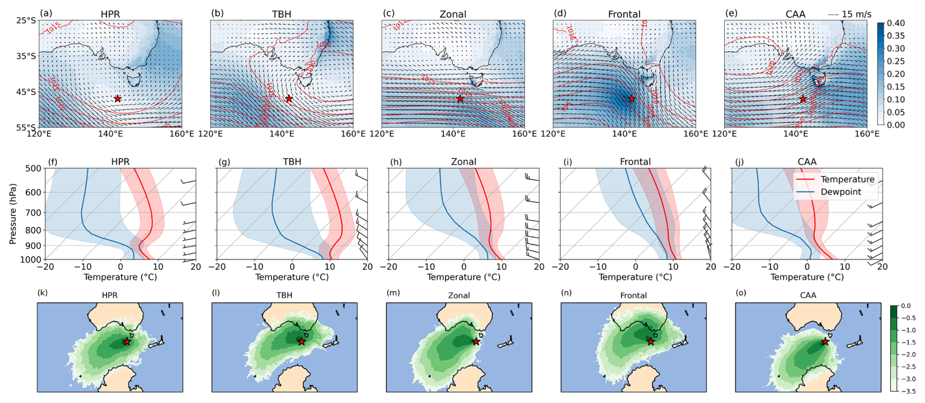
Figure 1 Characteristics of synoptic regimes: (a–e) Spatial distributions of precipitation (shaded, unit: mm h⁻¹), mean sea-level pressure (MSLP, contours, unit: hPa) and wind (vector, unit: m s⁻¹) at 975 hPa over the SO for five major synoptic types during 1990–2023. The red mark in the figure represents the location, 47° S and 142° E, where the IMOS buoy is deployed. (f–j) Composite of Skewt-Logp thermodynamic diagram for synoptic types at SOFS calculated from ERA5. Red and blue lines represent mean profiles of temperature and dew point temperature, respectively, and the shaded region indicates their standard deviation. Wind barbs on the right of the figure indicate the speed and direction of wind at different pressure levels. (k–o) Probability density (on a logarithmic scale) of 72 h back trajectories of air parcels at 1000 m for the synoptic regimes at SOFS. Density is the number of trajectory visits per latitude–longitude grid cell, normalised by the total trajectory count for the respective regime.

All bulk parameterization algorithms utilize the Monin–Obukhov similarity theory (MOST) (Monin and Obukhov, 1954), which is expressed by the following equation:

$$\begin{array}{}\text{(1)}& \mathrm{SHF}=\mathit{\rho }\cdot C_p\cdot C_H\cdot U\cdot \left(\mathrm{SST}-\mathrm{AT}\right)\end{array}$$

where: ρ = Air density (kg m⁻³), C_p = Specific heat capacity of air (J kg⁻¹ K), C_H = Sensible heat transfer coefficient, U = Wind speed at reference height (m s⁻¹), SST = Sea surface temperature (K or °C), AT = Air temperature at reference height (K or °C).

$$\begin{array}{}\text{(2)}& \mathrm{LHF}=\mathit{\rho }\cdot L_v\cdot C_E\cdot U\cdot \left(q_{\mathrm{s}}-q_{\mathrm{r}}\right)\end{array}$$

where: ρ = Air density (kg m⁻³), L_v = Latent heat of vaporization (J kg⁻¹), C_E = Latent heat transfer coefficient (dimensionless), U = Wind speed at reference height (m s⁻¹), q_s = Specific humidity at the surface (kg kg⁻¹), q_r = Specific humidity at reference height (kg kg⁻¹).

2.3 Synoptic classification using K-means clustering on ERA5 data

The K-Means is one of the simplest and non-hierarchical clustering techniques based on vector quantization developed by Hartigan and Wong (1979). The technique requires two inputs: (1) the number of clusters (k) and (2) the initial random positions of each cluster's centroids. Each measurement is assigned to its nearest centroid, and the centroids are then updated iteratively based on the cluster's values. To minimize the sum of squared deviations inside clusters, the operation is repeated until the centroid positions settle. For this study, ERA5 hourly data from 2010 to 2023 is employed to perform K-means clustering of weather types at the SOFS location. Following Lang et al. (2018), the K-means incorporates four variables (temperature, RH, u, and v) at three levels (925, 850, and 700 hPa), along with three surface variables (pressure, AT, and RH). Before clustering, each variable is normalized (resulting in zero mean and unit standard deviation).

2.4 Calculating inversion strength and M-index

The EIS (Wood and Bretherton, 2006) is defined as:

$$\begin{array}{}\text{(3)}& \mathrm{EIS}=\mathrm{LTS}-{\mathrm{\Gamma }}_{\mathrm{m}}\left(Z_{\mathrm{700}}-Z_{\mathrm{LCL}}\right).\end{array}$$

In this equation, LTS represents Lower Tropospheric Stability (θ₇₀₀−θ₀) (Klein and Hartmann, 1993), θ and Z denote potential temperature and geopotential height, respectively. The subscripts “700”, “0”, and “LCL” correspond to the 700 hPa level, 1000 hPa level, and Lifting Condensation Level, respectively. Γ_m signifies the moist adiabatic θ gradient at 850 hPa, calculated using the average temperature between the 1000 and 700 hPa levels. The M-index (Kolstad and Bracegirdle, 2008) evaluates boundary layer stability and is an important indicator of cloud formation characteristics in high-latitude regions. The M-index highlights air–sea potential-temperature contrasts, ie, the potential temperature difference between the surface and 850 hPa, and is closely tied to surface flux forcing, making it a better predictor of cloud-boundary (base/top) heights (Naud et al., 2020). In contrast, EIS is a capping-inversion strength metric that correlates more weakly with cloud boundaries (Naud et al., 2020), but correlates strongly with cloud fraction (Wood and Bretherton, 2006).

2.5 Himawari-8 data

Lang et al. (2022) used Advanced Himawari Imager (AHI) Himawari-8 geostationary meteorological satellite data (Bessho et al., 2016) to categorise open and closed MCC using Convolutional Neural Network (CNN) models from the TensorFlow Python package. They trained the model utilising hourly brightness temperature data with 5 km resolution from channel 11, which operates at a wavelength of 8.6 µm and subsequently applied for MCC classification from 2016 to 2021. Our study utilised the MCC data from Lang et al. (2022) over SOFS, with a 1 h time resolution and 5 km spatial resolution. We defined the open and closed MCC at SOFS as the respective cloud types occupying 80 % or more of the 2.5° × 2.5° box centred on the site.

2.6 HYSPLIT model data

The 72 h back-trajectories were computed at an altitude of 1000 m above SOFS using the Hybrid Single-Particle Lagrangian Integrated Trajectory (HYSPLIT) model (Draxler and Hess, 1998) to investigate the origins of air masses during different synoptic conditions. Hourly data from ERA5 served as the input for the meteorological parameters utilised in the back trajectory modelling. HYSPLIT requires both surface and pressure level fields, which are provided through two ERA5 files: a 2D file (containing surface variables such as mean sea-level pressure, 2 m temperature, 10 m horizontal wind componets and bounday layer height etc) and a 3D file (containing meteorological variables on pressure levels, including horizontal wind components, pressure vertical velocity, temperature, and humidity etc.) (NOAA HYSPLIT Users Guide – S141, https://www.ready.noaa.gov/hysplitusersguide/S141.htm, last access: 5 December 2025). These files were combined and converted into the HYSPLIT-specific ARL format, which was then used as the input for trajectory calculations.

3 Results

3.1 Characteristics of synoptic types and air-sea interaction over the SO

Located roughly midway between Tasmania and the SO storm track, the SOFS site (star in Fig. 1a; 47° S, 142° E) experiences meteorology dominated by passing mid-latitude cyclones and fronts (Rudeva et al., 2019). K-means clustering of meteorological variables at SOFS identifies five synoptic weather regimes that align with the first five clusters found in Truong et al. (2020). To fix the cluster number to 5, we analysed cluster numbers ranging from 3 to 8 based on circulation patterns and thermodynamic profiles. The elbow method suggests that four clusters would be a suitable choice as they adequately explain much of the structural variability (Fig. S2, Supplement); however, this approach presents a limitation. Specifically, opting for four clusters didn't capture the Tasman Blocking High, an important synoptic feature situated near the SOFS (Figs. 1 and S2). In contrast, the fifth cluster effectively identifies the Tasman Blocking High, completing a comprehensive synoptic classification of the weather regimes. We now discuss the dynamic and thermodynamic features of these weather regimes, as well as the characteristics of air-sea interactions at the SOFS.

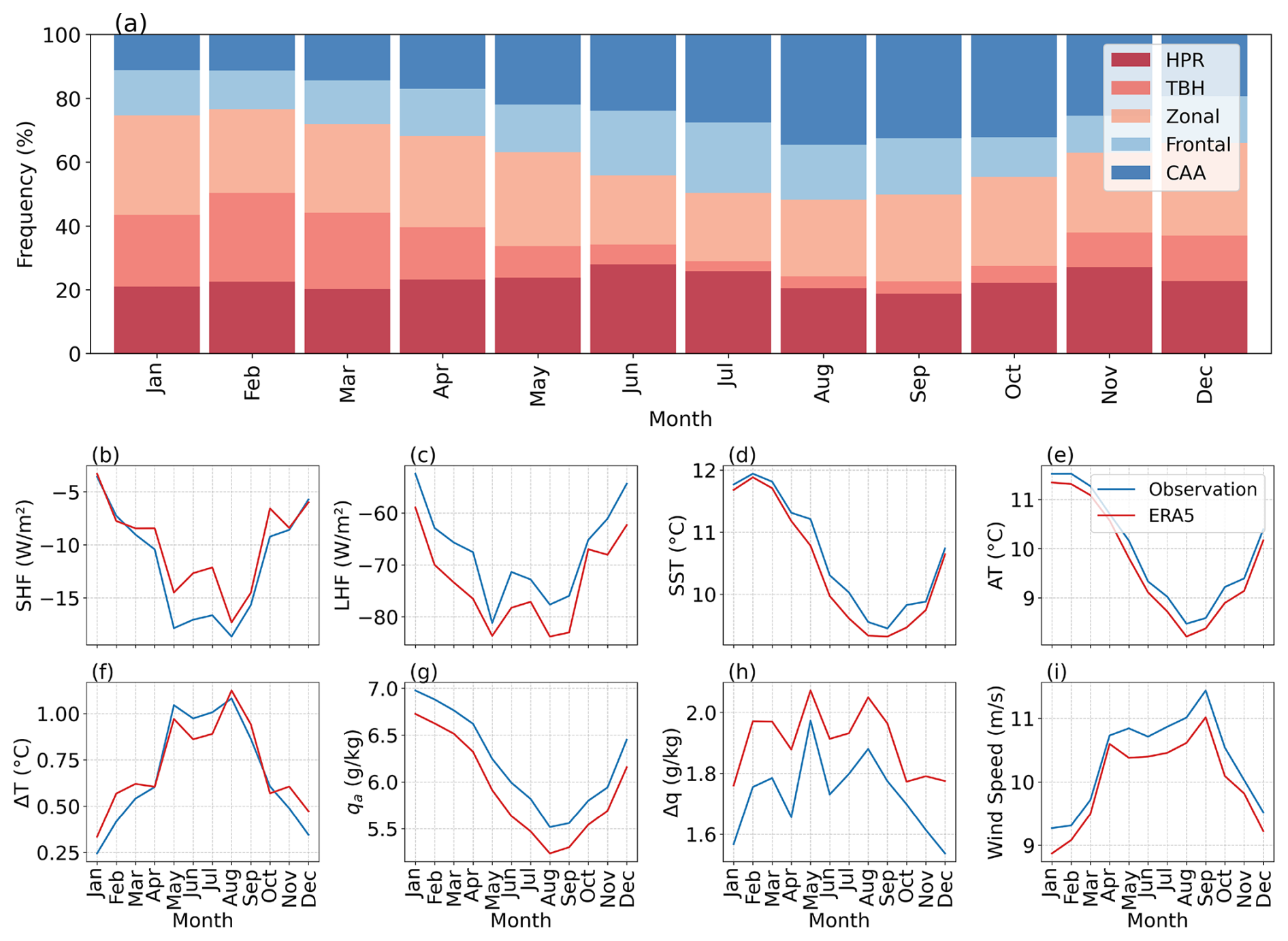
Figure 2 Seasonality: (a) Seasonality of synoptic regimes at the SOFS. (b–g) Seasonality of SHF and LHF and their drivers at SOFS.

High Pressure/Ridging (HPR), frequency of occurrence 22.9 %: The HPR is characterised by a weak circulation pattern (Fig. 1a) and demonstrates no observable seasonality over the SOFS (Fig. 2a). This weather regime represents an extension of the high-pressure belt over southern Australia, marked by light precipitation rates (0–0.025 mm h⁻¹) in ERA5 at SOFS. In contrast, a significant amount of precipitation is observed southwest of SOFS. Analysis indicates that HPR is associated with an elevated LCL at 937 hPa and a pronounced temperature inversion starting at 900 hPa. The back-trajectory results (Fig. 1k) reveal that air masses typically reach the SOFS site from the west during the HPR, which aligns with the vertical profile of horizontal wind depicted in Fig. 1f.

Tasman Blocking High (TBH), frequency of occurrence 12.0 %: The TBH reflects a blocking anticyclone over the Tasman Sea (Risbey et al., 2009). It demonstrates a pronounced seasonal cycle, with a maximum frequency during the summer (Fig. 2a). The wind profile shows moderate intensity with a consistent northwesterly direction (Fig. 1b). Similar to HPR, the ERA5 surface precipitation rate is weak during TBH conditions, and the centre of the intense precipitation is located southwest of SOFS. The thermodynamic profile Fig. 1g highlights that, relative to HPR, the temperature inversions in TBH start from a lower level itself (nearly from 950 hPa). Notably, the TBH has a warmer and wetter atmosphere at the surface level, resulting in a mean LCL at 966 hPa. This weather regime is often associated with air masses originating from the northwest sector of the SOFS, indicating a continental influence (Fig. 1l).

Zonal, frequency of occurrence 26.6 %: The zonal is the most frequent synoptic weather regime over SOFS and exhibits no seasonality. The composite MSLP and circulation for the zonal regime depicts a widespread subtropical ridge over south of Australia with strong westerly winds at SOFS (Fig. 1c). The SkewT-LogP diagram reveals a moderate temperature inversion from 850 hPa. The trajectories in Fig. 1m indicate that the predominant source of air masses associated with this regime originates from the west of the SOFS.

Frontal, frequency of occurrence 15.5 %: The frontal cluster represents a seasonal cycle, characterised by its maximum occurrence during the winter months (Fig. 2a). This regime features strong north-westerly winds driven by a low-pressure trough south of SOFS. It includes the warm conveyor belt of the mid-latitude cyclones along the storm track (Fig. 1d, n). Frontal soundings show a near-saturated atmosphere from 1000 to 850 hPa, with the LCL at 965 hPa, resulting in the most intense precipitation at SOFS. Specifically, ERA5 indicates a precipitation rate of 0.35–0.40 mm h⁻¹ during the frontal passage through SOFS.

Cold Air Advection (CAA), frequency of occurrence 22.6 %: The CAA is the dominant wintertime synoptic regime, with a frequency of approximately 30 % in August. The maximum CAA frequency in winter is associated with a northward shift of the subtropical ridge and associated intrusion of cold airmass from the far south of SOFS (Hoskins and Hodges, 2019). This weather regime is related to post-frontal conditions, with the high-pressure centre located northwest of the SOFS (Fig. 1e). During CAA, the SOFS encounters the south-westerly winds of a pristine SO airmass (Fig. 1e, o), associated with cold air outbreaks. The surface is extremely dry, with a dewpoint depression of nearly 8 °C and the mean LCL extending to 912 hPa.

Table 1 Comparison of SHF and LHF mean and median values (unit: W m⁻²) from buoy observations and ERA5 across different clusters.

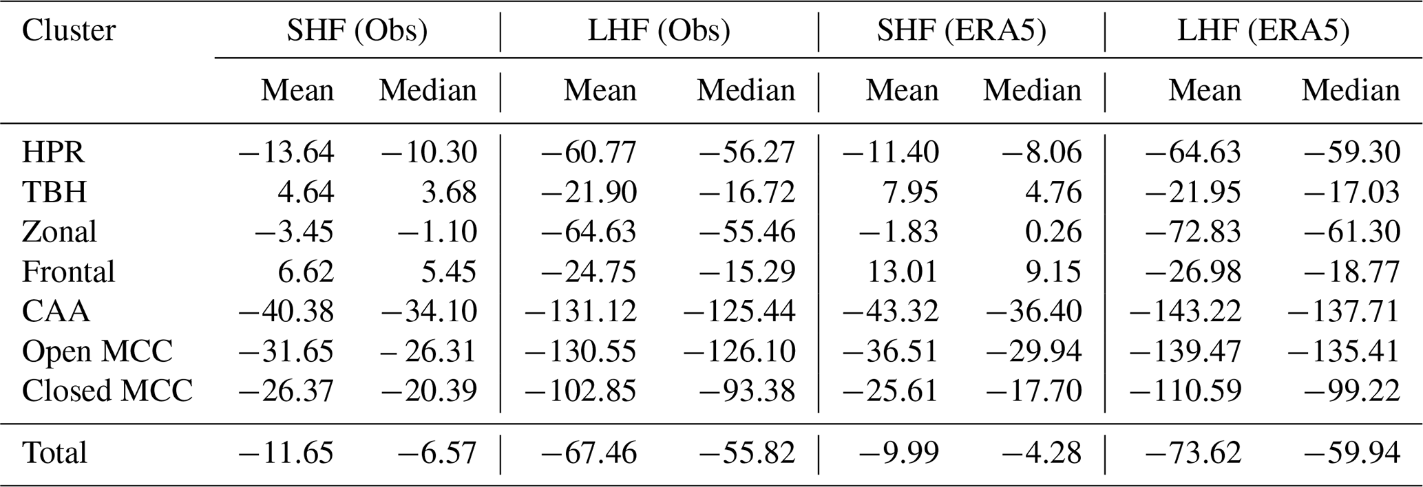
In this section, we analyse the characteristics of air-sea interaction at SOFS. As indicated in Table 1, the mean SHF and LHF at SOFS are −11.6 and −67.5 W m⁻², respectively, suggesting that LHF is approximately 5.8 times greater than SHF. Observational data and ERA5 reanalysis reveal a significant increase in both SHF and LHF from May to September (late autumn to early spring) period (Fig. 2b, c). Over this time, SST and AT reach their minimum values; however, their gradient reaches a maximum of nearly 1° C (Fig. 2f). This pronounced SST-AT gradient (ΔT), along with increased wind speed, results in a peak in SHF (as shown in Fig. 2i). Similarly, the LHF peak during late autumn to early spring is driven by a large humidity gradient (Δq, Fig. 2h) between q_s and q_a and stronger wind conditions at SOFS.

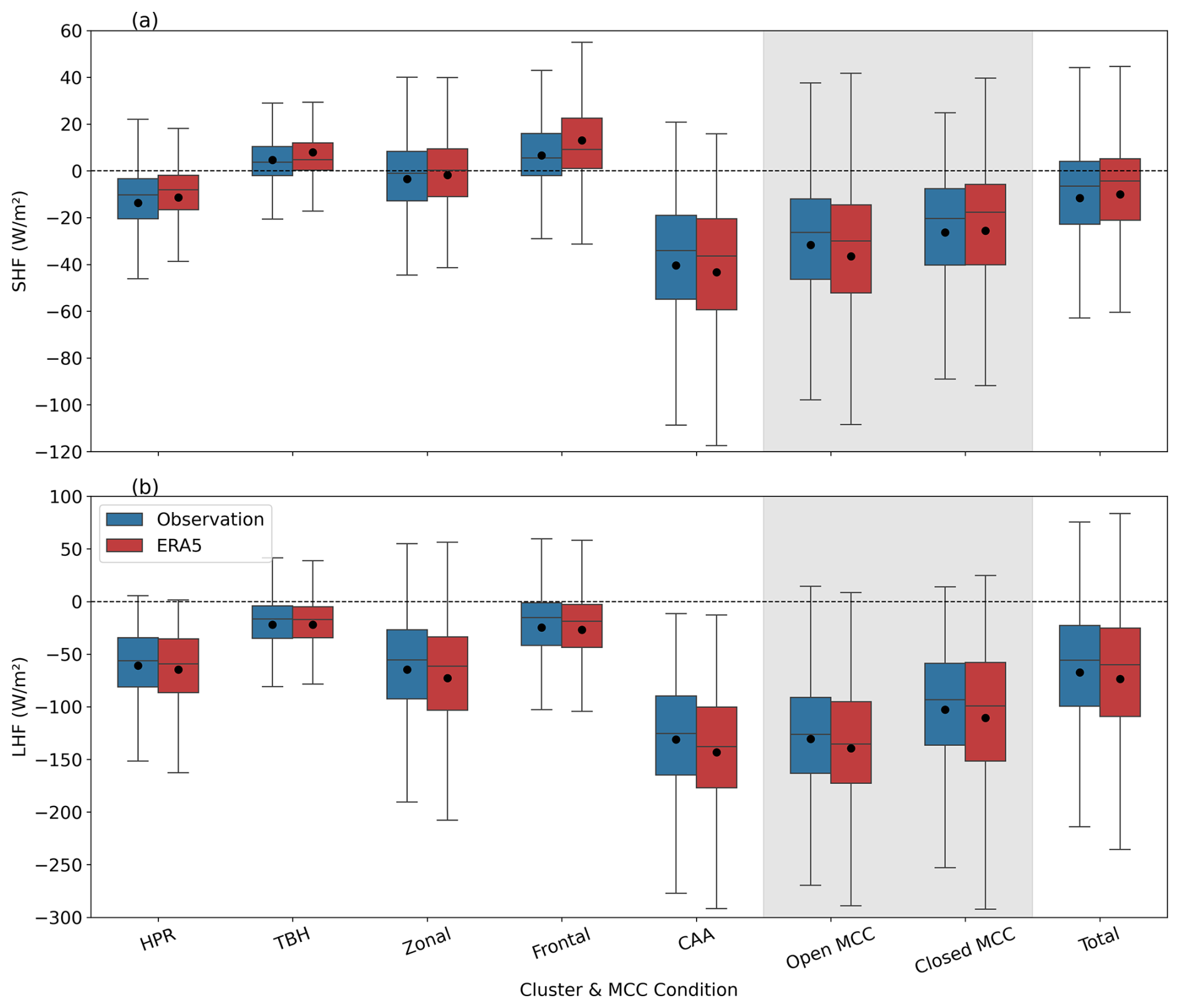
Figure 3 Synoptic regimes and air-sea interaction: Box plots for (a) SHF and (b) LHF from the buoy and ERA5 corresponding to different synoptic types and all cases of open/closed MCC condition at SOFS. The horizontal line within the box represents the median (50th percentile), and the black dots represent the mean of the distribution.

3.2 Changes in air-sea interactions associated with synoptic types over SO

Surface fluxes, including the SHF and LHF, are key variables related to the coupling between the ocean and the atmosphere. Figure 3 illustrates that the surface flux exchange varies considerably across different synoptic types, and CAA is associated with the maximum SHF and LHF exchange (Papritz et al., 2015). During CAA events, the mean SHF and LHF reached maxima of −40.4 and −131.1 W m⁻², respectively, which are approximately 3.5 and 2 times greater than the overall mean (Fig. 3a and b; Table 1). The cold and dry southerly winds characteristic of this regime result in a pronounced decrease in AT and q_a (Fig. 4b, d). This leads to a stronger temperature and humidity gradient at the surface (Fig. 4c, e), facilitating substantial heat and moisture transfer from the ocean. Consistent with previous studies (Fletcher et al., 2016a, b), the CAA exhibits the highest M index (mean = −1.3 K) and the lowest EIS (mean = 1.4 K), indicating increased instability and a weaker temperature inversion compared to other weather regimes at the SOFS (Fig. 5e). For CAA, the correlation between surface fluxes and the M-index is strongest when EIS < 0 (sample sizes by EIS condition: Table S1), with R² values of 0.48 for SHF vs. M-index and 0.41 for LHF vs. M-index. Furthermore, the change in surface fluxes with the M-index is more pronounced when EIS < 0, measured at −12.1 W m⁻² K⁻¹ for SHF and −19.8 W m⁻² K⁻¹ for LHF. When EIS > 0, or when there is a stronger capping inversion, the variance in surface fluxes explained by the M-index diminishes, or the surface flux–M relationship weakens (Fig. 5e, j). The observed tendencies in SHF/LHF with M and EIS support the notion that weak inversions reduce capping, thereby promoting the coupling or effective transfer of moisture/heat from the boundary layer to the free troposphere (Wood and Bretherton, 2006; Galewsky, 2018), which enhances the efficiency of surface flux increase with the M-index. Conversely, stronger inversions lead to decoupling, insulating the boundary layer from the free troposphere and thus reducing the sensitivity of surface fluxes to the M-index.

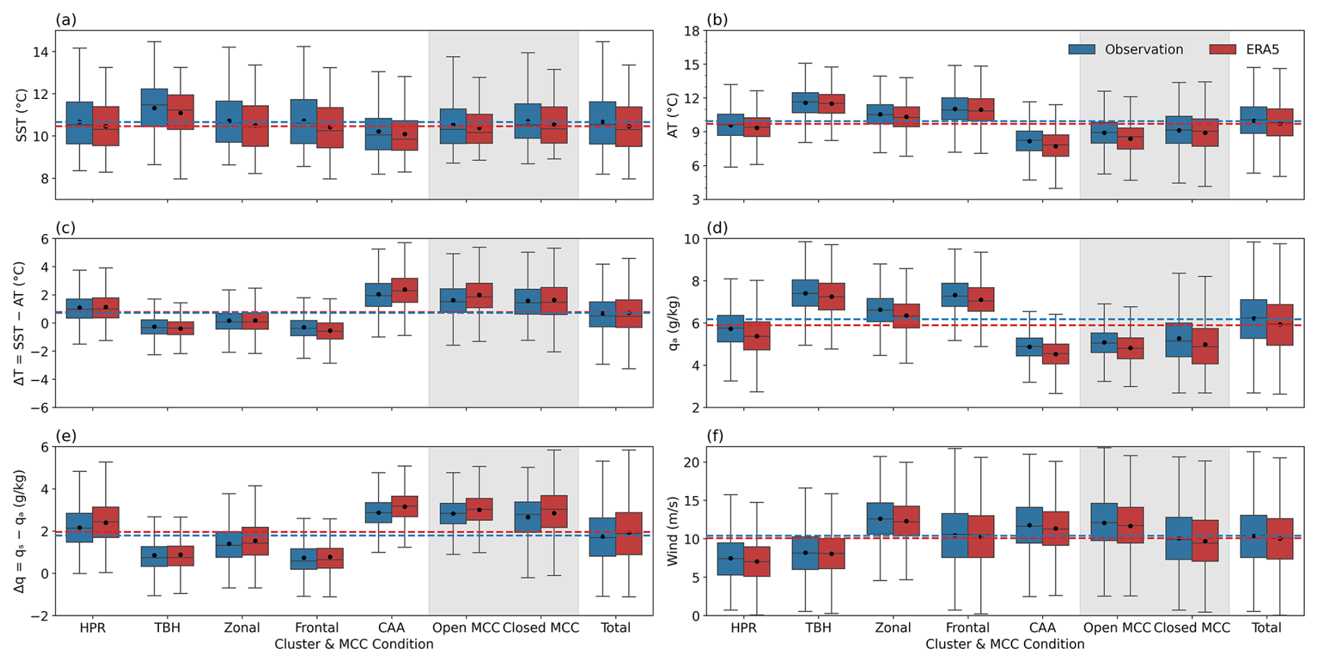
Figure 4 Influence of synoptic regimes on surface meteorology: Box plots of (a) SST, (b) AT, (c) ΔT, (d) q_a, (e) Δq and (f) wind speed for synoptic types and all cases of open/closed MCC condition at SOFS from buoy and ERA5. The horizontal line within the box represents the median (50th percentile), and the black dots represent the mean of the distribution. The red and blue horizontal dotted lines represent the overall means of each variable from ERA5 and buoy, respectively.

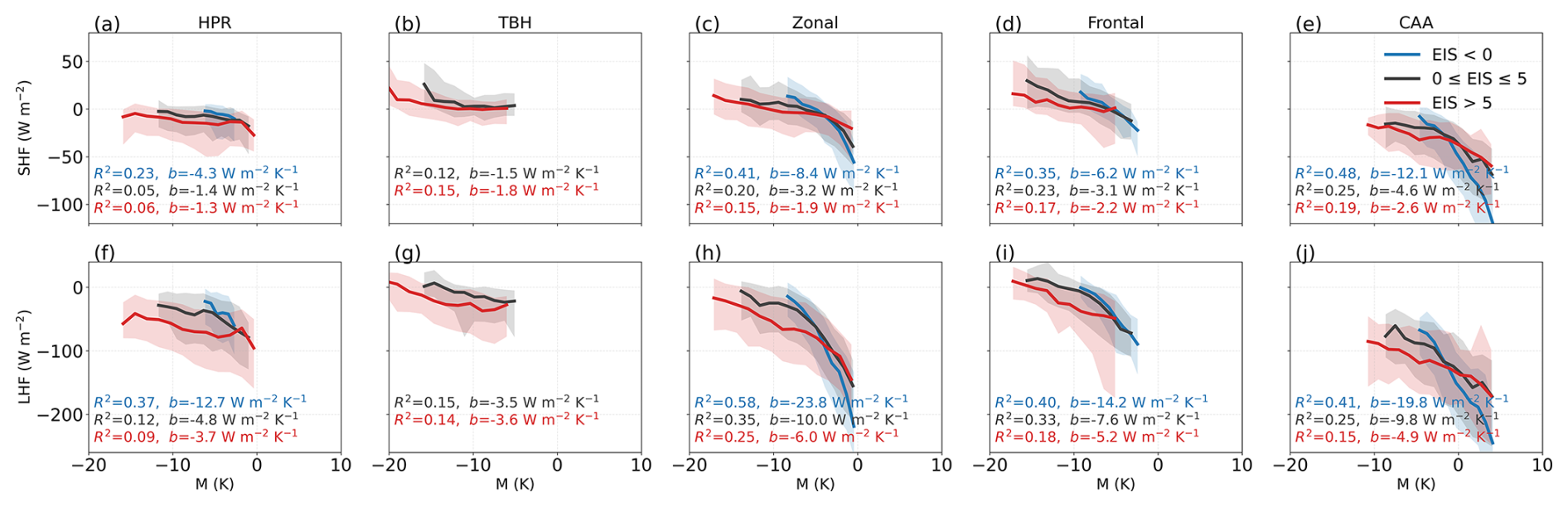
Figure 5 Surface flux relationships with stability indices by synoptic regime at SOFS. (a–e) SHF relationship with M-index and EIS for the five synoptic regimes. Solid lines show median SHF computed in 20 equal-width M-index bins within each regime. Curves are conditioned on EIS (blue: EIS < 0 K; gray: 0 ≤ EIS ≤ 5 K; red: EIS > 5 K). Shaded bands denote the 10th–90th percentile of SHF in each M-index bin. Panel annotations report the linear-regression slope b (unit: W m⁻² K⁻¹) and coefficient of determination R² for each EIS class. (f–j) As in panels (a)–(e), but for LHF. SHF or LHF cases with fewer than 100 samples in a given EIS category were excluded from the analysis.

The HPR regime has a mean SHF and LHF of −11.6 and −56.8 W m⁻², and these relatively weak fluxes are attributed to the lower temperature and humidity gradients, coupled with the weak surface wind conditions illustrated in Fig. 4. The HPR is characterised by a stable atmosphere, with a mean M-index of −8.0 K and an EIS of 6.2 K. Analysis reveals that there is no strong relationship between the surface fluxes and the M-index for this weather regime, as evidenced by an R² value of less than 0.1 for the M-index versus SHF relationship. For TBH and frontal clusters, the mean SHF transfers from the atmosphere to the ocean (Fig. 3a and Table 1), associated with warm air advection originating from the northwest sector of the SOFS. This finding is consistent with Naud et al. (2021), who noted that surface fluxes are either weak or transfer from the atmosphere to the ocean in the warm sector of extratropical cyclones. The warm air advection from lower latitudes increases the AT (Fig. 4b), thereby facilitating a negative SST-AT gradient as illustrated in Fig. 4c. Figure 3b reveals that TBH and frontal clusters exhibit minimal LHF exchange from the ocean, driven by a relatively moist near-surface atmosphere (Fig. 4d) and a considerably low moisture gradient (Fig. 4e). The M-index and EIS have a mean value of −12.9 and 7 K, respectively, in TBH, and the relationship between these indices and surface fluxes appears to be weak as depicted in Fig. 5b and g. Conversely, during the frontal regime, surface fluxes increase with the M-index, and their relationship is stronger under lower inversion values (EIS < 0), with R² of 0.35 for SHF vs. M and 0.40 for LHF vs. M.

The distribution of SHF within the zonal cluster suggests an equilibrium state in the heat exchange process, induced by a neutral thermal gradient, as depicted in Fig. 4c. Within this zonal regime, the mean value of the M-index is recorded at −7.1 K, while the EIS is 3.1 K. The relationship between fluxes and the M-index becomes significantly stronger under weak inversions, with an R² of 0.41 for SHF vs. the M-index and 0.58 for LHF vs. the M-index. Furthermore, the rate of LHF exchange with respect to the M-index is maximum within this regime (when EIS < 0), where LHF changes at a rate of −23.8 W m⁻² K⁻¹ relative to the M-index.

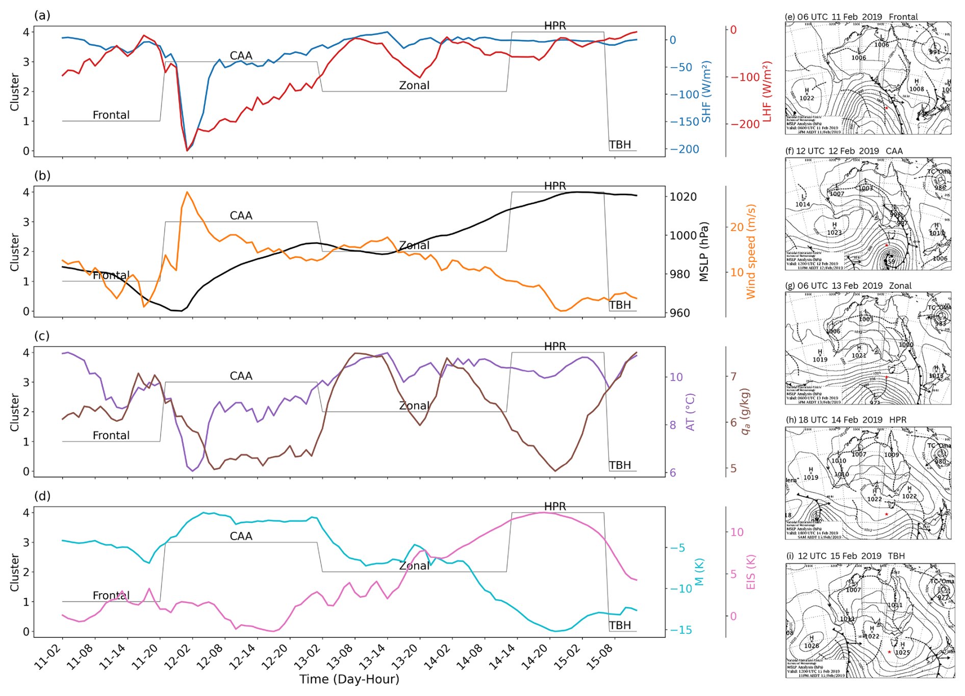
Figure 6 Case study: Time series of (a) SHF and LHF, (b) MSLP and wind speed, (c) AT and q_a, (d) M-index and EIS during the transition from one cluster (synoptic regime) to another. (e–i) Spatial distribution of MSLP for synoptic regimes (source: Bureau of Meteorology). The red star indicates the location of the IMOS buoy.

The variations in SHF and LHF during the passage of a synoptic regime, along with associated changes in meteorology and air-sea interaction, are presented through a case study from 11 to 15 February 2019 (Fig. 6). It is evident that when transitioning from a frontal regime to CAA, there is a sharp increase in SHF and LHF with a noticeable decrease in MSLP, and an increase in surface wind speed (Fig. 6a, b). Following the passage of this regime, zonal regimes emerge, leading to a weakening of air-sea interactions. Other surface parameters, such as AT, q_a, and stability indices (M-index and EIS), closely mirror the observed patterns in Figs. 4 and 5 for all synoptic regimes noted at SOFS.

3.3 Influence of synoptic types on MCC and differences in air-sea interaction for open and closed MCC

The frequency of open and closed MCCs associated with synoptic types over the SOFS highlights that open MCCs are more prevalent during the CAA regime (Fig. 7a). In contrast, closed MCCs are more frequent in high-pressure weather regimes due to strong lower-tropospheric inversions (McCoy et al., 2017; Lang et al., 2022). Frontal systems increase atmospheric instability, making boundary layer clouds, like open and closed MCCs, less common (Fig. 7a). McCoy et al. (2017) identified significant differences in the ΔT values associated with open and closed MCCs, with open MCCs showing a larger ΔT compared to the closed ones. However, it is important to note that the geographical distribution of open and closed MCCs is notably different in their study. Open MCCs are mainly observed in the warmer waters of lower latitudes, whereas closed MCCs are frequently found at higher latitudes, where SST is generally lower. Thus, when cold air masses advect through relatively cooler SSTs prevalent in higher latitudes, this results in lower ΔT values, where the closed MCCs are frequent. In lower-latitude regions, cold air advection over warmer surface water results in higher ΔT, representing the dominant open MCC region in their research.

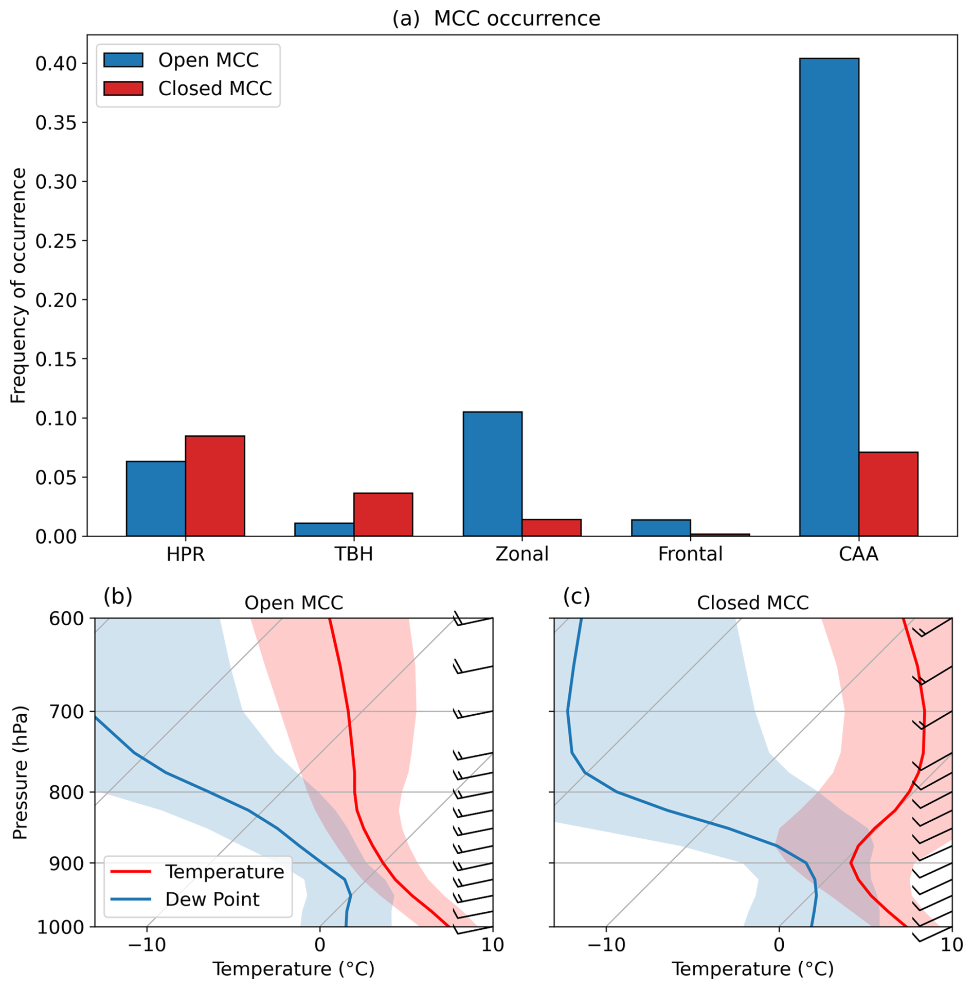
Figure 7 Influence of synoptic regimes on open and closed MCC: (a) The frequency of open and closed MCC occurrence is associated with synoptic types. (b, c) The composite of the Skewt-Logp thermodynamic diagram for all cases of open and closed MCC conditions.

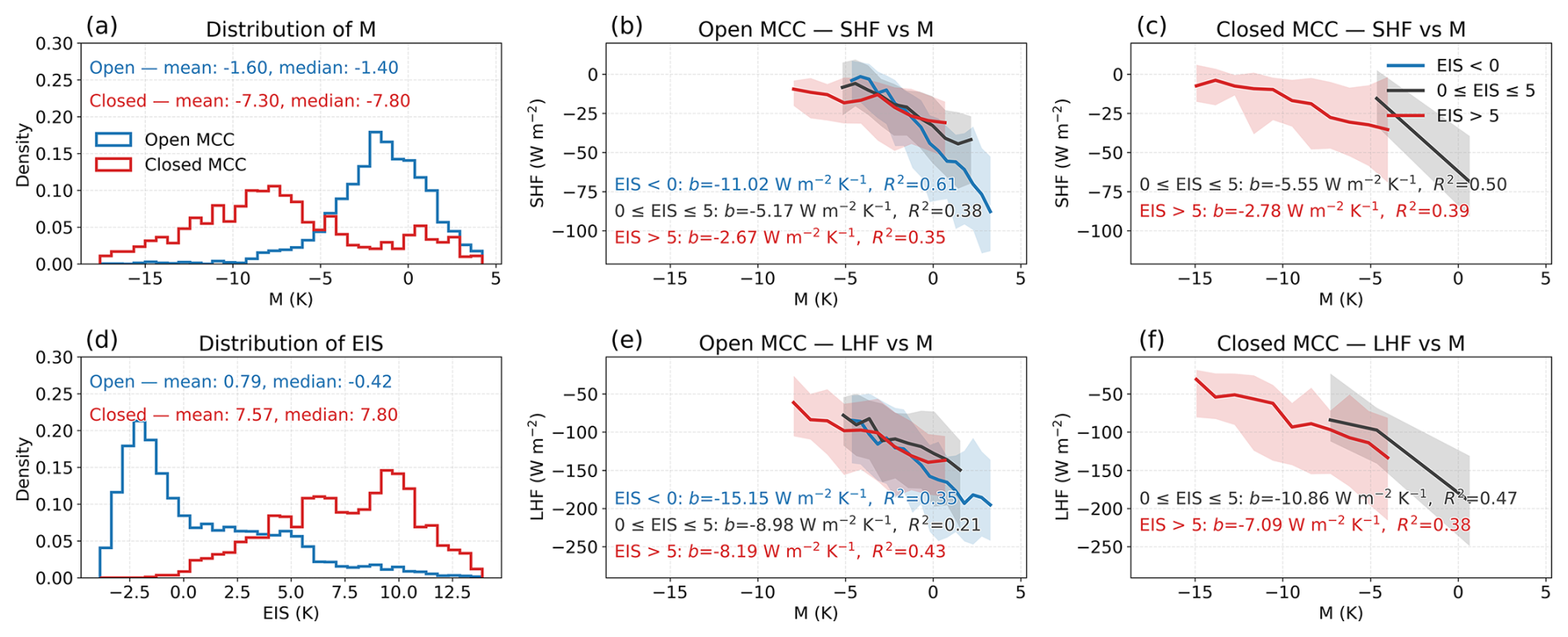
Figure 8 Stability index distribution and its relationship with surface fluxes: (a) Probability distribution of the M-index for all cases of open (solid blue) and closed (solid red) MCC at SOFS. (b, c) Relationship between SHF, M-index, and EIS for open and closed MCCs. Solid lines show SHF medians computed in 20 equal-width M-index bins for open and closed MCCs. Curves are conditioned on EIS (blue: EIS < 0 K; gray: 0 ≤ EIS ≤ 5 K; red: EIS > 5 K). Shaded regions denote the 10th–90th percentile range of SHF within each M-index bin. Panel annotations indicate the linear-regression slope b (unit: W m⁻² K⁻¹) and coefficient of determination R² for each EIS class. (d) Same as panel (a), but for EIS. (e, f) Same as panels (b) and (c), but for LHF. SHF or LHF cases with fewer than 100 samples in a given EIS category were excluded from the analysis.

When considering all open and closed MCC cases at the same location, i.e., SOFS, in contrast to McCoy et al. (2017), we noted that ΔT and Δq have similar distributions for open and closed MCCs (Fig. 4). However, the wind speed exhibits a difference between these two cloud types, with open MCCs demonstrating higher wind speeds, primarily due to their more frequent occurrence in the stronger wind regime, i.e., CAA (Figs. 4f and 7a). Similarly, open MCCs display moderately stronger mean SHF and LHF values (−31.6 and −130.6 W m⁻²) compared to closed MCCs (−26.4 and −102.8 W m⁻²; Table 1, Fig. 3). Importantly, the comparison of fluxes within a regime under both open and closed MCC conditions reveals similar SHF or LHF between the two cloud types (Fig. S3, Supplement). So the analysis confirms that moderate differences in fluxes observed across all cases of MCC types are due to variations in the occurrence frequency of these cloud types within specific weather regimes. The open and closed MCCs differ primarily in EIS and the M-index, considering all cases and specific weather regimes (Figs. 8 and S3). The open MCC clouds are characterised by a mean M-index of −1.6 K and EIS of 0.8 K, whereas closed MCC conditions are associated with a stable atmosphere, with a mean M-index of −7.3 K and EIS of 7.6 K (Fig. 8a, d). Thus, beyond the surface fluxes, the M-index and EIS may play a more significant role in determining the cellular characteristics of these clouds, particularly when these clouds are evaluated in the same geographical location.

In both open and closed MCC conditions, the SHF–M relationship strengthens as the capping inversion weakens. For open MCC, the R² value increases from 0.38 to 0.61 as EIS decreases from 0–5 K to less than 0 K; during this transition, the regression slope becomes steeper, changing from −5.1 to −11.0 W m⁻² K⁻¹. This suggests that when EIS is below 0 K, a 1 K increase in the M-index results in approximately twice the increase in SHF compared to when 0 ≤ EIS ≤ 5 K. Similarly, in closed MCC, as EIS decreases from values above 5 K to between 0 and 5 K, the R² between SHF and M increases from 0.39 to 0.50, and the SHF–M slope becomes steeper, shifting from −2.8 to −5.6 W m⁻² K⁻¹. For LHF, the variance explained by M changes more modestly with EIS in open MCC. Nonetheless, the sensitivity still increases under weaker inversions: the LHF–M slope steepens from −9.0 to −15.2 W m⁻² K⁻¹ as EIS decreases from 0–5 K to less than 0 K.

3.4 Evaluation of ERA5 Fluxes with SOFS Measurements

A comparison of the mean observed fluxes with ERA5 with its nearest grid point reveals that ERA5 underestimates the observed SHF by 1.7 W m⁻² and overestimates the LHF by −6.2 W m⁻² (Fig. 3 and Table 2). The primary factor contributing to the SHF underestimation is the negative bias in wind speed within ERA5, where the mean ΔT is approximately 0.75 °C, closely aligning with the observed value (Fig. 4c, f). The negative bias in SHF is pronounced during the austral winter (June–August), coinciding with the peak negative bias in wind speed (Fig. 2i). Conversely, during the summer months (December to February), ERA5 SHF closely matches the observed SHF. Analysing the factors underlying the mean LHF overestimation reveals that ERA5 exhibits a significant dry bias in near-surface specific humidity compared to observations, resulting in a stronger Δq (which is 2 g kg⁻¹ in ERA5, whereas in observations, it is 1.8 g kg⁻¹). This enhanced moisture gradient compensates for the negative bias in wind speed, leading to an overestimation of the ERA5 LHF (Figs. 3b and 4d, e, f). The bias in ERA5 LHF varies monthly and is primarily influenced by fluctuations in Δq (see Fig. 2c, h). Overall, ERA5 effectively captures variations in SOFS fluxes, as evidenced by strong correlation coefficients of r = 0.90 (p < 0.01) for SHF and r = 0.92 (p < 0.01) for LHF.

Table 2 Root mean square error (RMSE, unit: W m⁻²), bias (unit: W m⁻²), and correlation of SHF and LHF from ERA5 compared to buoy observations across different clusters.

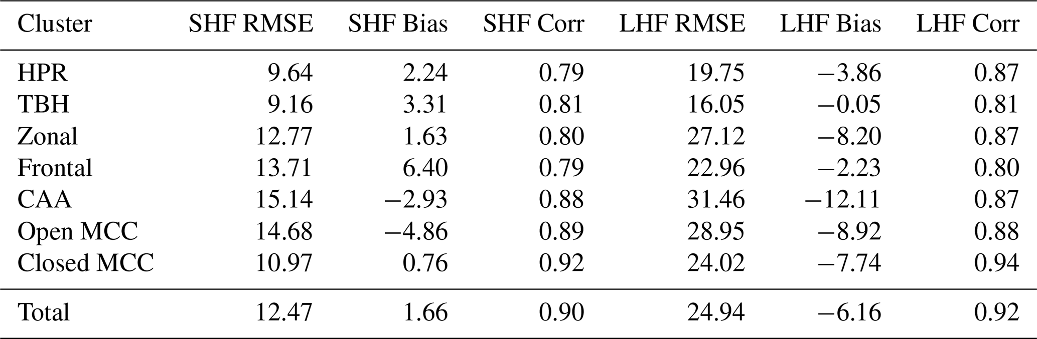
Figure 3 illustrates that the accuracy of ERA5 fluxes varies across different weather regimes. During CAA, there is a notable overestimation of the SHF and LHF, with mean biases of −2.9 W m⁻² for SHF and −12.1 W m⁻² for LHF (Table 2). These biases in SHF and LHF are comparatively lower than the surface flux biases of approximately 100 W m⁻² reported by Seethala et al. (2021) during intense cold air outbreaks over the Gulf Stream. The SHF overestimation in ERA5 during the CAA regime is attributed to a positive bias in the ΔT, which is +0.4 °C warmer than the observations. Similarly, the overestimation of ERA5 LHF during CAA is affected by a drier surface level and a larger Δq in ERA5 (Fig. 4d, e). Despite these overestimations, ERA5 fluxes exhibit a strong relationship with observed fluxes during CAA events, with correlation coefficients of r = 0.88 (p < 0.01) for SHF and r = 0.87 (p < 0.01) for LHF. For TBH and frontal regimes, ERA5 overestimates SHF from the atmosphere to the ocean, with mean biases of 3.3 and 6.4 W m⁻², respectively. Notably, the mean bias for ERA5 LHF in the TBH regime is −0.05 W m⁻², and it is the smallest bias in SHF observed across all synoptic regimes at the SOFS. The most frequently observed zonal clusters indicate a mean SHF bias of 1.6 W m⁻² and an LHF bias of −8.2 W m⁻², with correlation coefficients of r = 0.80 (p < 0.01) for SHF and r = 0.87 (p < 0.01) for LHF (Table 2).

The evaluation of surface flux for open MCC (Table 2) shows that the ERA5 and observed fluxes have a high correlation coefficient, measuring 0.89 (p < 0.01) for SHF and 0.88 (p < 0.01). At the same time, ERA5 shows a mean bias of −4.9 W m⁻² for SHF and −8.9 W m⁻² for LHF, which are driven by positive bias in ΔT and Δq, respectively. For the closed MCC period, ERA5 SHF exhibits a minimal bias of 0.8 W m⁻², accompanied by a strong correlation of 0.92 (p < 0.01). The ERA5 and observed ΔT are similar for closed MCC, while the wind speed displays a negative bias. For this cloud type, the ERA5 LHF exhibits the highest correlation of 0.94 (p < 0.01) with observations, accompanied by a bias of −7.7 W m⁻². Although the closed MCC conditions exhibit an improved ΔT bias compared to open MCC periods, the Δq bias remains unchanged, leading to a persistent LHF bias. In summary, the ERA5 demonstrates significant skill in reproducing observed fluxes overall, across the synoptic regimes and under both open and closed MCC conditions at SOFS.

4 Discussion and conclusion

We identified five weather regimes over the SOFS buoy's site: HPR, TBH, Zonal, Frontal, and CAA. The different synoptic regimes significantly impact the modulation of SHF and LHF over the SO (Fig. 3). Not surprisingly, the CAA episodes are associated with intense SHF and LHF release from the ocean, tied to the influx of dry and cold air from the high latitudes south of SOFS. The TBH cluster is characterised by relatively weak air-sea interaction, indicative of warm and moist air advection from the northwestern sector of the SOFS. When the EIS is less than zero, both SHF and LHF exhibit significant linear correlations with the M-index across the CAA, zonal, and frontal regimes (Fig. 5). In the zonal regime, the relationship between LHF and the M-index is characterised by an R² value of 0.58 and a slope of −23.8 W m⁻² K⁻¹, which is the highest among all regimes analysed. Notably, across these regimes, the slope of the surface flux versus M-index relationship more than doubles when the inversion strength transitions from 0 ≤ EIS ≤ 5 K to EIS < 0. This indicates an increased sensitivity of SHF/LHF to the M-index under unstable stratification, which is consistent with enhanced air–sea coupling and surface flux exchange between the boundary layer and free troposphere. The HPR and TBH regimes represent a stable atmosphere, where the relationship between the SHF/LHF and the M-index is relatively weak.

Given the primary role that MABL clouds play in the Earth's radiation budget, it has long been a priority to understand the mechanisms that govern the transition of cloud morphology from one state to another. In the subtropics, increases in SHF and LHF have been identified as critical factors in the transition from stratocumulus to trade cumulus clouds (Wyant et al., 1997; Sandu and Stevens, 2011) along a Lagrangian trajectory. However, when considering all cases of open and closed MCC, our findings indicate that open MCCs are associated with a mean SHF of −31.6 W m⁻² and LHF of −130.5 W m⁻², while closed MCCs are associated with a mean SHF of −26.4 W m⁻² and LHF of −102.8 W m⁻². Therefore, the closed and open MCC states exhibit relatively small variations in SHF and LHF (1.2 % and 1.3 %, respectively), and this difference primarily arising from changes in the occurrence frequency of these cloud types within a specific weather regime. Thus, the results suggest a limited role for these fluxes in the transition of these MABL clouds when measured at the same geographical location. From the Eulerian perspective of the SOFS, SST, and AT undergo only weak variations between cloud morphological states (Fig. 4a and b).

The LHF are of further importance in constraining the water budget over the SO, given that a precipitation rate of 1 mm d⁻¹ is balanced by the evaporation from an LHF of ∼ 28.9 W m⁻² over the cold waters of the SO. Currently, there are significant discrepancies in the intensity and spatial distribution of precipitation products across the SO (Manton et al., 2020; Boisvert et al., 2020; Behrangi and Song, 2020; Montoya Duque et al., 2023), mainly due to the scarcity of high-quality observations in this remote and harsh environment (Siems et al., 2022). A study by Alinejadtabrizi et al. (2024) at the Kennaook/Cape Grim observatory (∼ 620 km northeast of SOFS) reported that the average precipitation rate (P) of open MCCs is 1.7 mm d⁻¹. In contrast, closed MCCs exhibited a rate of 0.3 mm d⁻¹. However, at SOFS, ERA5 indicates a precipitation rate of 1.6 mm d⁻¹ for open MCC and 0.7 mm d⁻¹ for closed MCC. Applying the ERA5 precipitation rates to the observed fluxes reveals a disparity between evaporation (E) and precipitation in open and closed MCCs at the SOFS location. Specifically, for closed MCCs, the evaporation equivalent of the LHF, E, is 3.4 mm d⁻¹, resulting in $E-P=\mathrm{3.4}-\mathrm{0.7}=\mathrm{2.7}$ mm d⁻¹. This indicates that water is being added to the MABL during periods of closed MCC. Assuming that specific humidity remains steady over time, the entrainment of dry, overlying air is necessary to maintain equilibrium in the specific humidity in the MABL. In the case of open MCC, $E-P=\mathrm{4.2}-\mathrm{1.6}=\mathrm{2.6}$ mm d⁻¹, it also adds significant water to the MABL, necessitating the transport of dry air from the free troposphere. The closed MCC is characterised by a strong inversion at approximately 900 hPa (Fig. 7c), and the inversion for open MCC is weaker and occurs at a higher altitude (∼ 820 hPa), allowing more active convection (Fig. 7b). The entrainment rate (w_e), calculated using the approximation $w_{\mathrm{e}}=E-P/(q_{\mathrm{ft}}-q_{\mathrm{s}})$, is 4.3 cm s⁻¹ for closed MCC, which is much larger than the entrainment rate in open MCC, i.e., 1.6 cm s⁻¹ (q_ft is the specific humidity in the free troposphere and q_s is the specific humidity at the surface from ERA5). The steeper moisture gradient between the surface and the lower free troposphere results in reduced entrainment in open MCC, whereas the weaker moisture gradient in closed MCC leads to a more intense entrainment rate than in open MCC. Our results are consistent with the findings of Berner et al. (2011, 2013), who showed through numerical simulations that entrainment is weaker in pockets of open cells because reduced turbulence at the cloud top limits mixing compared to the surrounding overcast stratocumulus field.

The findings indicate that ERA5 surface fluxes effectively represent SOFS bulk fluxes, demonstrating strong correlations for both SHF and LHF, although SHF is slightly underestimated while LHF is overestimated. The underestimation in SHF is linked to the underestimation of wind speed in ERA5, given that the ΔT is nearly identical in both observations and ERA5. However, the dry bias in q_a drives a pronounced moisture gradient between the ocean and the near-surface atmosphere in ERA5, which compensates for the underestimation of wind speed, resulting in an overall overestimation of LHF. The performance of ERA5 fluxes varies across different synoptic regimes; frontal regimes exhibit the maximum bias in SHF (6.40 W m⁻²), CAA shows the maximum LHF bias (−12.1 W m⁻²) at SOFS. For both open and closed MCC cloud patterns, the ERA5 fluxes are highly reliable, and the performance is slightly better during closed MCC. The better performance of ERA5 in representing the fluxes during closed MCC compared to open MCC may suggest challenges in representing shallow precipitating convection in ERA5 (Zheng and Miller, 2022; Dai, 2024; Jeon et al., 2023), whereas closed MCCs are better represented with the large-scale parameterisation of clouds. This, in turn, would affect SST, AT and q_a, and consequently, surface fluxes.