Assessing the skill of high-impact weather forecasts in southern South America: a study on cut-off lows

Cut-off lows (COLs) are mid-tropospheric cyclonic systems that frequently form over southern South America, where they can cause high-impact precipitation events. However, their prediction remains a challenging task, even in state-of-the-art numerical weather prediction systems. In this study, we assess the skill of the Global Ensemble Forecast System (GEFS) in predicting COL formation and evolution over the South American region where the highest frequency and highest intensity of such events are observed. The target season is austral autumn (March to May), in which the frequency of these events is at its maximum. Results show that GEFS is skillful in predicting the onset of COLs up to 3 d ahead, even though forecasts initialized up to 7 d ahead may provide hints of COL formation. We also find that as the lead time increases, GEFS is affected by a systematic bias in which the forecast tracks lie to the west of their observed positions. Analysis of two case studies provides useful information on the mechanisms explaining the documented errors. These are mainly related to inaccuracies in forecasting the vertical structure of COLs, including their cold core and associated low-level circulation. These inaccuracies potentially affect thermodynamic instability patterns (thus shaping precipitation downstream) as well as the horizontal thermal advection which can act to reinforce or weaken the COLs. These results are expected to provide not only further insight into the physical processes at play in these forecasts, but also useful tools for the operational forecasting of these high-impact weather events over southern South America.

1 Introduction

Severe weather phenomena can significantly impact densely populated regions (e.g., Curtis et al., 2017; Newman and Noy, 2023; Sanuy et al., 2021). Over southern South America, these are frequently associated with heavy-precipitation events triggered by low-pressure systems known as cut-off lows (COLs; Campetella and Possia 2007; Godoy et al., 2011a; Muñoz and Schultz, 2021). COLs are synoptic-scale weather systems that originate from elongated cold troughs in the middle troposphere, which subsequently detach (“cut off”) from the main westerly current (Palmén and Newton, 1969). This segregation from the main flow explains the isolated and erratic behavior of these systems, which poses a significant challenge in operational weather forecasting, even for state-of-the-art numerical weather prediction (NWP) systems (Muofhe et al., 2020; Yáñez-Morroni et al., 2018). Naturally, this can have an impact on the reliability of weather forecasts and early warnings, which may be particularly relevant to southern South America considering it is remarkably affected by COLs (Godoy et al., 2011a).

Previous studies have focused on quantifying the explicit forecast errors associated with COLs in NWP systems. Gray et al. (2014) examined forecast ensembles from three operational forecast centers in the Northern Hemisphere and found that forecast errors were systematically larger in COL compared to non-COL events for the same prediction time. Similarly, Saucedo (2010) conducted an assessment of the prediction skill of the Global Forecast System (GFS) and Weather Research and Forecasting (WRF) models in southern South America for three COL events. His results indicated that forecast accuracy varies significantly depending on the individual COL cases and emphasized the need for an accurate representation of the COL center position during initialization to achieve better forecast results.

Other studies, such as those from Muofhe et al. (2020) and Binder et al. (2021), have linked errors in precipitation forecasts with inaccuracies in the location of the COL centers. In their evaluation of Météo-France forecasts, Binder et al. (2021) analyzed a single COL event and documented an eastward shift in both precipitation and COL position, primarily due to an initial underestimation of the COL intensity. Meanwhile, Muofhe et al. (2020) assessed the skill of the NWP model currently used operationally at the South African Weather Service to simulate five COL events. They observed variations in the predictive skill of COL-related precipitation across different development stages of the COLs, attributing these differences to inaccurate positioning of their centers. Moreover, studies by Bozkurt et al. (2016), Yáñez-Morroni et al. (2018) and Portmann et al. (2020) have underscored the influence of the COL-induced circulation on extreme precipitation events, emphasizing the complexity and challenge of predicting these phenomena. In particular, Portmann et al. (2020) noted in a case study that uncertainties in the COL genesis position substantially affect the vertical thermal structure and subsequent evolution of surface cyclone development.

While previous studies have examined the skill of NWP systems in forecasting COLs, they usually cover a short period of time and do not address a compound evaluation of positional and intensity errors. For instance, a recent paper by Lupo et al. (2023) has quantified biases in COL forecasts globally but for the operational version of the GFS model in a 7-year period running from 2015 to 2022. In this context, there is a necessity to deepen our comprehension of COL predictive skill given the close linkage with heavy-rainfall events. Our study tries to fill this gap, focusing on southern South America, a hotspot region for COL development (e.g., Reboita et al., 2010; Godoy, 2012, henceforth GD12; Pinheiro et al., 2017).

Our main goal is to assess the prediction skill of COLs in the National Centers for Environmental Prediction (NCEP) Global Ensemble Forecast System (GEFS). This is achieved through quantifying forecast errors using an objective feature-tracking methodology which involves the identification and tracking of COLs along the forecast trajectories to produce a set of forecast versus observed COLs.

In this study, we specifically address three aspects of COLs: their onset time, their central position and their intensity. In particular, we seek to respond to the following questions:

1. What is the temporal scale at which GEFS can reliably predict the initiation phase of COLs, and how precise are these forecasts?

2. After formation, can GEFS accurately predict the subsequent trajectories of the COLs?

3. Can errors in COL forecasts impact those of precipitation further downstream?

It should be noted that this study can be considered a first step towards a full characterization of the physical mechanisms controlling the forecast skill of COLs and how the associated errors in state-of-the-art NWP systems are transferred to other associated variables such as precipitation, atmospheric instability and winds. The rest of the paper is organized as follows: the datasets and methodology are described in Sect. 2. The results on the forecast skill of the GEFS in both COL onset and their evolution stages are included in Sect. 3, followed by a summary and the concluding remarks in Sect. 4.

2 Data and methodology

2.1 The GEFS Reforecast dataset

Daily averages from the GEFS Reforecast version 2 dataset (Hamill et al., 2013) are used as a representative sample of the GEFS model for the purpose of this study. This dataset consists of 11 ensemble members – 1 control run alongside 10 perturbed members – and covers a prediction horizon of 16 d after initialization. During the first week, data are saved at 3-hourly intervals considering a horizontal resolution of T254 (roughly 40 km × 40 km at 40° latitude) and 42 vertical levels. The GEFS Reforecast dataset can be freely downloaded from https://downloads.psl.noaa.gov/Projects/Reforecast2/ (last access: 10 March 2025), where the reforecasts have been saved at 1° × 1° horizontal resolution from the native-resolution data. It is worth noting that for all calculations within the paper, we considered the ensemble mean to be the basis for analysis and comparisons (i.e., no assessment is performed on individual ensemble members). To validate the GEFS skill, we use the fifth version of the ECMWF Reanalysis dataset (ERA5; Hersbach et al., 2020) as a representation of the real-world conditions. The ERA5 data, with an original resolution of approximately 0.25° × 0.25°, were coarsened to the same resolution as that of the reforecast to ease comparison.

Our analysis focused on the forecast verification of atmospheric variables at the 300 hPa level. This level was chosen because it hosts both the largest frequencies and the highest intensities of COLs within the Southern Hemisphere (e.g., Reboita et al., 2010; Pinheiro et al., 2021). To detect COLs, we analyzed the geopotential height and the zonal wind component at 300 hPa as well as the 300–850 hPa thickness. We also evaluated other variables of interest such as the geopotential height at 850 hPa and the total accumulated precipitation to represent the lower-level circulation and related impacts of COLs.

2.2 Temporal domain and study area

The temporal domain of our study is based on the availability of reforecast data, ranging from 1985 to 2020. Specifically, we focus on the austral autumn season, covering the months of March, April and May, which is the season with the highest frequency of COLs in South America (Reboita et al., 2010; Pinheiro et al., 2017; Muñoz et al., 2020). Regarding the spatial domain, we focused on the area of greatest occurrence of COLs, which encompasses the western side of southern South America (Reboita et al., 2010; Campetella and Possia, 2007; GD12). Specifically, we utilized the area situated between latitudes 37.6 and 29.9° S and longitudes 77.6 and 68.75° W, as illustrated in Fig. 1. This region has been extensively studied in the past by GD12, who found that the COLs in this area are particularly strong and can often cross the Andes Mountains, leading to conditions prone to high-impact weather events over the continent further downstream (Godoy et al., 2011a).

Figure 1 Spatial distribution of COLs in the region of highest COL frequency in southern South America from 1985 to 2020. Black crosses represent the start of trajectories of COLs detected in the study area (37.6–29.9° S and 77.6–68.75° W, solid black box), and lines represent their trajectories with colors representing the duration of each COL.

2.3 COL identification and tracking algorithm

The COL dataset from GEFS and ERA5 is built following the approach outlined by GD12 and based on the conceptual framework of COL by Nieto et al. (2005). This conceptual model characterizes a COL as a closed cyclonic circulation isolated from the main westerly current and characterized by a cold core at mid-levels.

To detect COLs, the tracking algorithm uses the geopotential height and the zonal wind component at 300 hPa as well as the 300–850 hPa thickness, following a series of steps to classify potential grid points as COLs: (1) in order to detect the closed circulation, the algorithm looks for local minima in the 300 hPa geopotential height field. It selects a grid point that is at least 5 geopotential meters (gpm) lower than six of the eight surrounding grid points to ensure a higher geopotential height. If this condition is not met, the algorithm checks that 14 out of the 16 surrounding grid points have a higher or equal value within 20 gpm of the candidate grid point. (2) To ensure that the system is isolated from the westerly current, the algorithm requires changes in wind direction in at least six grid points located south of the candidate grid point. (3) Finally, to confirm the presence of a cold core, the algorithm employs the 300-850 hPa thickness as an indicator of temperature. It searches for a local minimum in thickness at the candidate point, following a procedure similar to the one used in the initial detection step. If a cold core is not found, the algorithm iterates through the eight surrounding grid points, accounting for possible displacements of the cold core relative to the geopotential minimum, as described in previous studies.

For validation purposes, we performed a visual inspection of the ERA5 COL outputs. This visual check confirmed that each event aligns with the conceptual model proposed by Nieto et al. (2005). Additionally, we stipulated that each COL should be identifiable for a minimum of 2 d in the reanalysis data. A total of 34 events met all the established criteria.

Following the identification of the COLs, we validated the GEFS COL dataset by comparing it with the ERA5 COL dataset. A GEFS COL was considered to correspond to the same system as a COL in the ERA5 dataset if their initial positions and respective trajectories satisfied predefined spatial and temporal criteria. The forecasted COL trajectories that met these criteria were used to generate diagnostics, quantifying errors in predicted positions, intensities and other properties of the COLs. The spatial criterion required that the distance between the forecasted and reanalysis trajectories did not exceed 800 km – this threshold was chosen based on the typical diameter of COL systems, which ranges between 600 and 1200 km (Kentarchos and Davies, 1998). Notably, our spatial criterion primarily focuses on the initial segment of the forecast trajectories rather than the entire track, consistent with the methodology of Froude et al. (2007a). This approach is justified by the expectation that forecast accuracy is generally higher at the start of the trajectory, where GEFS trajectories are likely to be more closely aligned with their ERA5 counterparts. Regarding the temporal criterion, a match was considered valid if at least one point along the system's life cycle coincided in time (i.e., within a 24 h period).

2.4 Verification metrics

For the quantification of the model skill, we used a Lagrangian perspective to derive error statistics. This methodology has been previously employed to build position and intensity error statistics in investigations on tropical and extratropical cyclones such as in Froude et al. (2007a, b) and Hamill et al. (2011). The validation metrics used in this study are sketched in Fig. 2 and are as follows:

• Direct positional error (DPE). This metric is defined as the horizontal distance between the observed and forecast positions at the same forecast time.

• Cross-track error (CTE). This metric represents the component of DPE that is perpendicular to the observed track. It provides information on the bias to the left or right of the observed track.

• Along-track error (ATE). This metric represents the component of DPE that is along the observed track. It provides information on the directional bias along the track, indicative of whether the forecasts predict a faster or slower motion of the system compared to the reanalysis.

We adopted the convention that a positive (negative) value of CTE indicates a bias to the right (left) of the observed track, while a positive (negative) value of ATE indicates that the model has a fast (slow) bias in its forecast track. It is important to note that CTE and ATE cannot be calculated for the first analyzed position of a COL since they depend on the existence of an observed position the day before the valid time. For a more detailed explanation of these metrics, see Heming (2017).

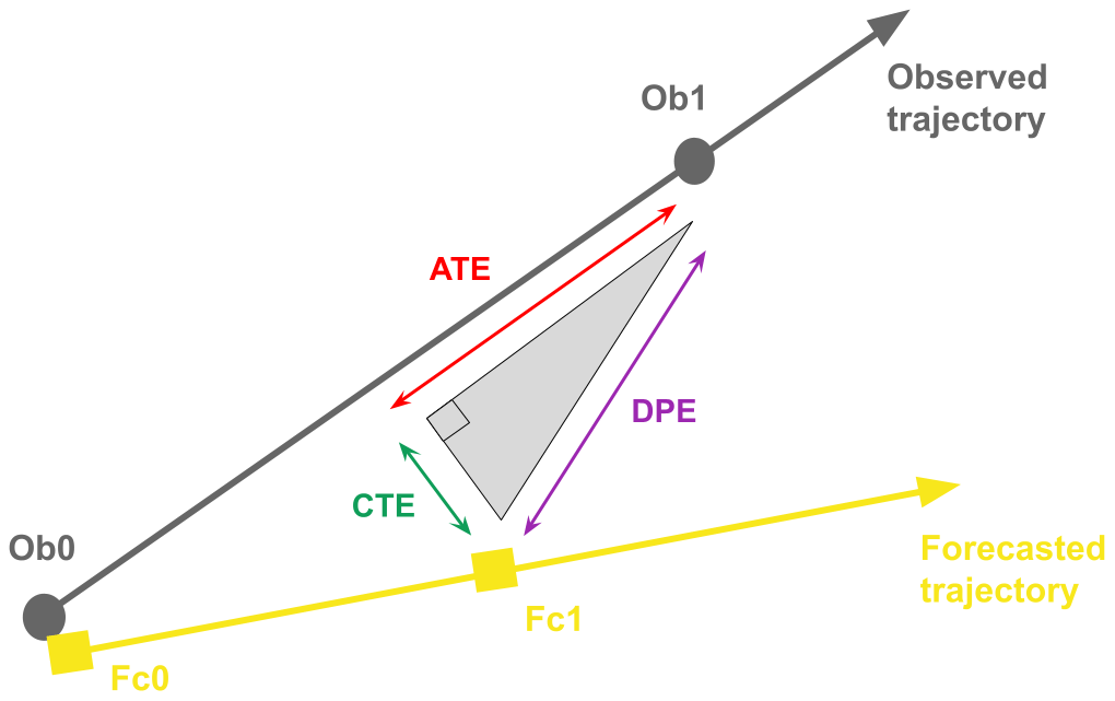
Figure 2 Measures of cyclone track forecast error: direct positional error (DPE; violet arrow), cross-track error (CTE; green arrow) and along-track error (ATE; red arrow). Ob0 and Ob1 are observed positions at times 0 and 1, while Fc0 and Fc1 are their respective forecasted positions. The gray circles (yellow squares) represent the observations (the forecasts).

3 Results

As a first step to determine the temporal horizon at which the GEFS model can forecast COLs, we analyze the central position of the COLs and their intensity. The intensity of COLs is defined by the maximum value of the Laplacian of the geopotential height field, where this maximum corresponds to the location of the COLs' centers. We present results for forecasts initialized up to 7 d prior to the observed onset of COL events, as the preliminary analysis indicated that no COLs were forecasted beyond this lead time. It should be noted that hereafter “onset stage” or “onset” of the COL refers to the beginning of the segregation stage, also known as stage 2 of the COL life cycle as defined by Nieto et al. (2005). We organized each forecast into eight groups based on their initialization day, namely init 0, init 1, init 2, init 3, init 4, init 5, init 6 and init 7. Forecasts labeled init 0 correspond to those initialized on the onset day of the COL, while forecasts labeled init 1 to init 7 indicate forecasts initialized 1 to 7 d before the onset day of the COL, respectively.

3.1 Predictive skill of COL onset time in GEFS

Figure 3 shows the percentage of detected COLs as a function of their initialization day, i.e., how many days in advance these systems could be forecasted in the GEFS dataset. During initializations closest to the onset days (init 0 to init 2), over 94 % of the total events (32 out of 34 COLs) were accurately predicted by the GEFS. However, this accuracy decreases significantly from init 3 onwards: 71 % at init 3, 56 % at init 4 and down to only 9 % at init 7. It is interesting to highlight, however, that the reforecasts were able to correctly predict most COLs on the same date they were observed, even when the initializations were farthest from the onset days (i.e., init 4 and init 5), indicating the accuracy of GEFS for predicting the timing of the events.

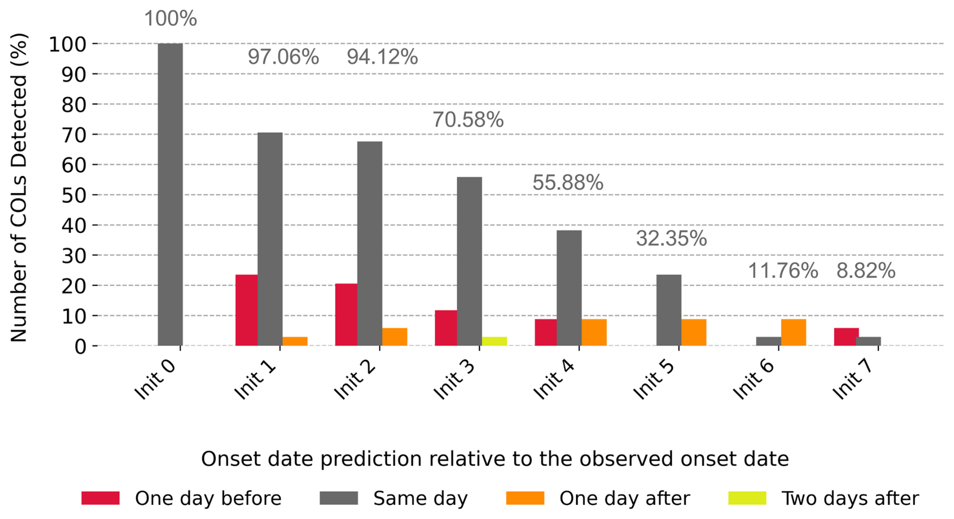
Figure 3 Percentage of forecasted COL initiations as a function of initializations, from init 0 (forecast initialized on the onset day) to init 7 (forecast initialized 7 d before the onset of the COL). The red, gray, orange and yellow bars indicate the forecasted date of the onset day of the COL relative to the observed date of the onset day, from 1 d ahead of formation to 2 d after, respectively.

Figure 4 illustrates the quartile distribution of the DPE and intensity error in the GEFS model for the onset day of the COLs, where each boxplot represents a different initialization day. The boxes represent the interquartile range (IQR), which comprises 50 % of the error distribution, with the median value indicated by a bold black line. Initially, a gradual increase in the median of DPE can be observed as the number of days before the onset of COL increases (Fig. 4a). The DPE increase varies from 140 km at the first initialization (init 0) to about 300 km at init 3. At the same time, the IQR expands from 300 km at init 1 to 900 km at init 3, indicating a widening spread of DPE with increasing forecast time. In contrast, the median of the intensity error exhibits a negative trend: it decreases from −2.5 gpm m⁻² at init 1 to −8 gpm m⁻² at init 3, with an IQR that varies significantly with the day of initialization. For subsequent initializations (init 5 to init 7), we observe a continuous increase in DPE from 400 km to approximately 600 km, alongside a consistent negative trend in intensity errors, with values around −13.0 gpm m⁻². However, it is important to note that these results are based on a smaller sample size than previous initializations and caution should be exercised when generalizing these results.

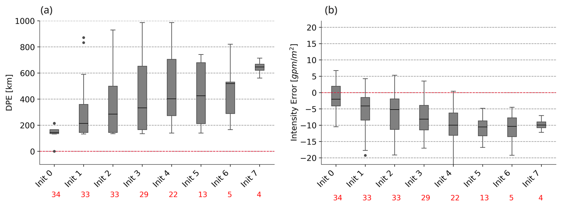
Figure 4 Variation in (a) the onset position (DPE) and (b) the intensity error as a function of initializations. The whiskers at the top (bottom) of the boxes represent the error's 75th (25th) quantile. The thick black horizontal lines inside the boxes represent the median (the 50th quantile), and the points outside the whiskers are considered outliers. The red numbers at the bottom indicate the number of systems identified under each initialization.

Figure 5 shows eight polar scatterplots illustrating the errors in the position of the predicted COLs in comparison to the reanalysis, with each plot corresponding to a particular initialization day. During the early initializations, the GEFS exhibits errors contained within a radius of 3° (approximately 300 km) around the observed positions and shows no discernible directional deviation. This indicates that the position errors are randomly distributed and show no systematic bias, which is particularly clear up to init 2. Meanwhile, initializations from init 3 to init 5 show a larger spread, with more points deviating significantly from the observed cyclone positions. While we detected a southward deviation, the zonal (i.e., east–west) behavior was less uniform, as init 3 showed a southern bias, init 4 a southwestern bias and init 5 a slight southwestern deviation. This indicates overall a slight deviation towards the south (on average between 1 and 3°), even if there is no clear longitudinal bias. Forecasts initialized with a larger lead time showed a larger spread, partly due to a smaller number of predicted COLs but also revealing a predominant southwesterly bias of the model.

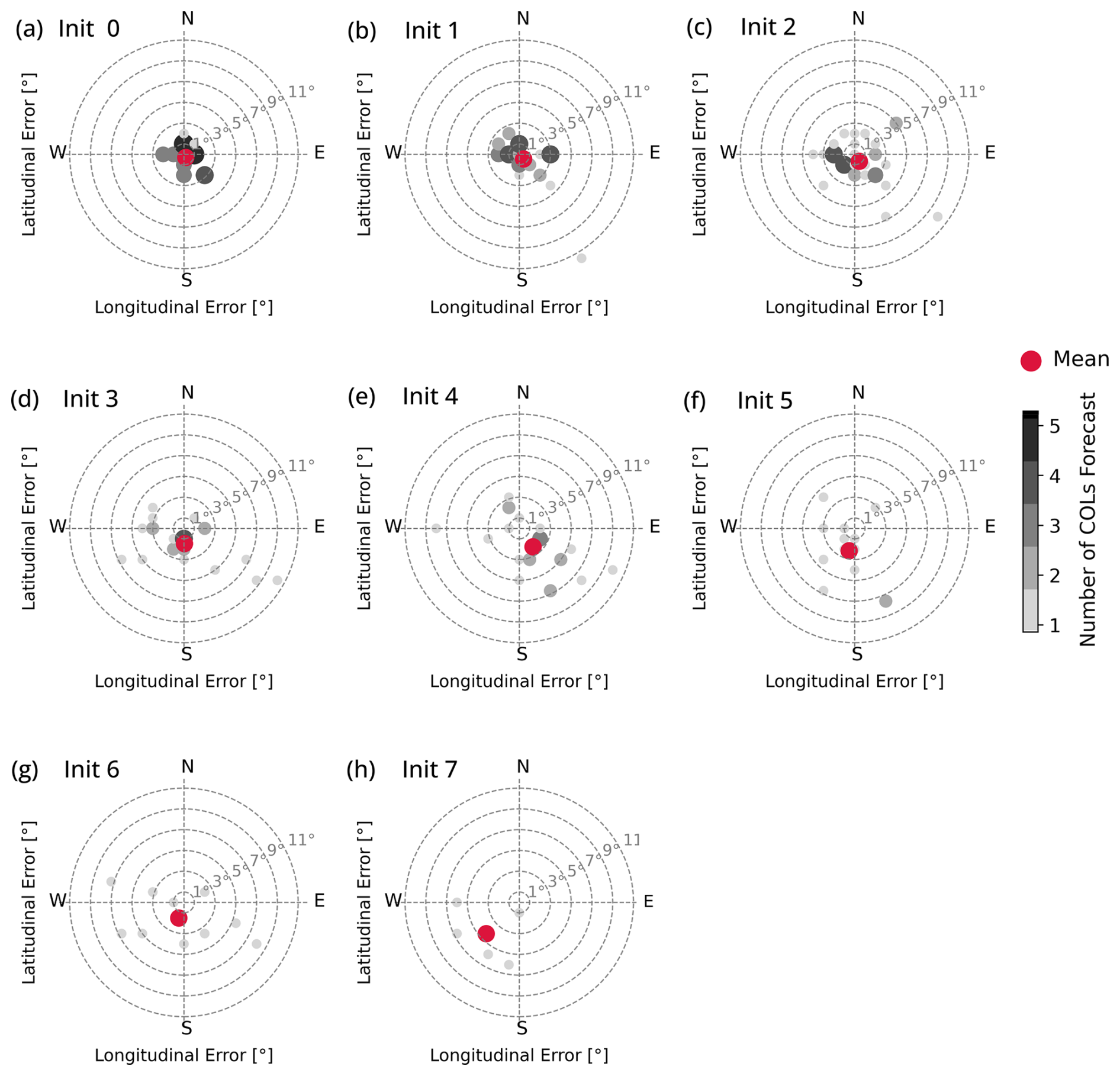
Figure 5 Scatter diagrams of COL initial position deviation decomposed in longitudinal and latitudinal errors (in degrees), where the central axis is the initial position observed. Each plot represents a different initialization, ranging from (a) init 0 (forecast initialized in the onset day) to (h) init 7 (7 d in advance). The gray and black dots indicate the location of the predicted COLs as a function of the initialization day (see the color bar for reference to the number of predicted systems per day). The red dots show the mean location after averaging all the COLs predicted on each initialization day.

3.2 Predictive skill of COL intensity and tracks in GEFS

In this section, we investigate whether there is any bias in predicting cyclone intensity, propagation speed and trajectory. We focused on the forecasts initialized up to 3 d before the segregation date since the number of detected cases is significantly lower for forecasts initialized beyond that point (i.e., init 4 to init 7), as explained in Fig. 3. Given that a preliminary study shows that a large portion of COLs in the study region have lifespans of 3–4 d or more, with nearly 80 % lasting beyond 3 d (not shown), we have focused our analysis on forecast lead times of up to 3 d following the initial detection of these COLs in the ERA5 reanalysis.

Figure 6 shows the quartile distribution of track errors, including DPE, ATE, CTE, and the intensity error between the GEFS and ERA5 trajectories for init 0 to init 3. Regarding DPE, each initialization shows similar sensitivity. For init 1 and init 2 (Fig. 6b, c), errors increase from 166 to over 320 km within 2 or 3 d of COL detection in the ERA5 reanalysis. The situation is similar for init 0 (Fig. 6a), where the error increases from 144 to over 275 km in the same period. Not surprisingly, init 3 (Fig. 6d) has the largest mean error, with a linear increase from 290 to 550 km. As regards IQR, it shows a linear increase, indicating that the dispersion of the position errors increases along the cyclone forecast period.

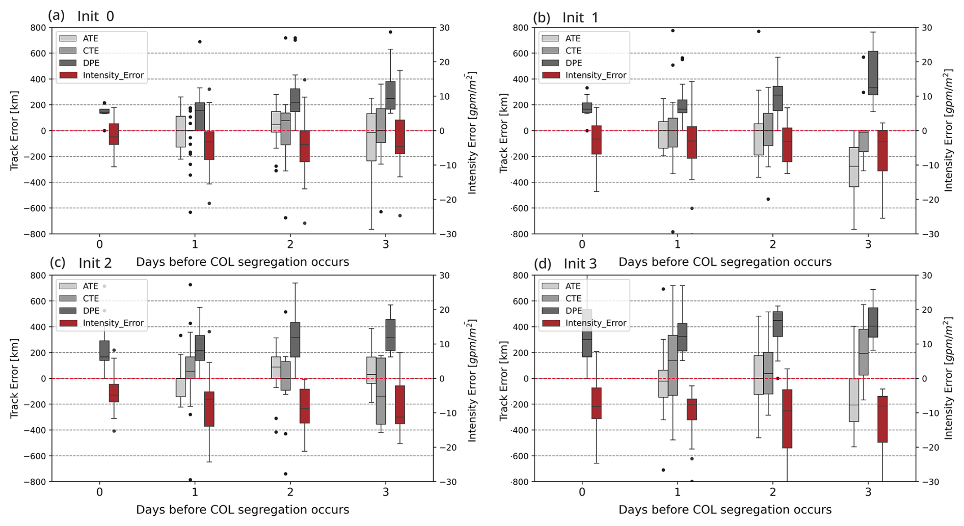
Figure 6 Boxplots of errors in track forecasts for DPE, ATE, CTE (on the left axis) and intensity (on the right axis) along the life cycle of the COLs. Each plot represents initializations at (a) init 0, (b) init 1, (c) init 2 and (d) init 3.

Conversely, a negative trend is observed in the intensity error and the corresponding ERA5 reanalysis trajectories. The magnitude of the error for init 0 and init 1 (Fig. 6a, b) initially increases from −2.0 to over −4.3 gpm m⁻² within 2 to 3 d of COL detection in the ERA5 reanalysis. For init 2 and init 3 (Fig. 6c, d), however, a further escalation of the error can be observed. While init 2 shows an increase in the magnitude of error from −4.9 to −11.68 gpm m⁻², init 3 shows an even more pronounced initial error of −8.14, which subsequently increases in its magnitude to −9.0 gpm m⁻². Regarding the dispersion of the error, it is noteworthy that init 1 and init 2 (Fig. 6b, c) show a slightly positive trend, indicating an increase in the uncertainty in the predicted system intensity. In contrast, the last initialization (Fig. 6d) shows significantly larger dispersion and a more variable behavior during the analyzed period. Despite the observed variability, however, a trend towards greater dispersion is discernible.

The ATE distribution exhibits a negative bias towards the later stages of the forecast trajectories, except for init 2 and init 0 (Fig. 6c), which show slightly positive values. Both init 1 and init 3 (Fig. 6b, d) exhibit negative biases with median distances of around 200 and 300 km, respectively. This negative bias in ATE may indicate that GEFS tends to underestimate the translational speeds of COL towards the latter stages of the forecast lead times. Regarding the CTE distribution (Fig. 6), no clear bias is observed; however, there are some noticeable trends in different initializations. In particular, init 2 (Fig. 6c) shows negative values at around 100 km. On the other hand, init 3 (Fig. 6d) displays predominantly positive values, representing a poleward bias according to its definition.

3.3 Case studies

In this subsection, we focus on two COLs that exhibited very different levels of prediction performance during their onset stage (Fig. 4a). The first case study, from March–April 2013, is characterized by small DPE values, below the first quartile in Fig. 4a, indicative of a forecast with high accuracy in the GEFS dataset. In contrast, the second case study, from March 2019, was associated with remarkably larger DPE values, with errors ranging between the median and the third quartile. This represents a scenario in which the prediction has a suboptimal performance. It is important to note that the selection of the case studies was based also on the impact model errors had on the associated precipitation downstream. For the analysis of precipitation, we considered the area of influence of the COLs approximately 7° (about ∼ 700 km radius) from the geopotential height minimum at 300 hPa. Before exploring the associated errors in the GEFS dataset, we provide a brief description of the synoptic environment around each COL during its segregation stage.

3.3.1 Case study 1: COL development on 31 March 2013

On 31 March 2013, a COL formed to the west of the Andes Mountains at 36° S and 75.5° W. Its lifespan lasted for 6 d, covering a distance of over 2000 km into the Atlantic Ocean (not shown). This event was associated with severe weather conditions which resulted in unprecedented flash floods in the region, leading to loss of lives, significant infrastructural damage and economic losses of USD 1.3 billion (Pink, 2018).

During the segregation phase of the COL, the main atmospheric features included an amplified ridge upstream of the system; the presence of two jet streaks – one to the north and one to the south of the COL; and a well-defined cold core in the middle levels (Fig. 7a, c). The COL extended towards the lower troposphere, where a closed cyclonic circulation can be observed, as indicated by the closed circulation at 850 hPa, directly beneath the COL at 300 hPa (Fig. 7c). Regarding the precipitation field, this COL led to high amounts of rainfall of over 25 mm d⁻¹ with peaks in excess of 50 mm in certain areas over south-central South America (Fig. 7b).

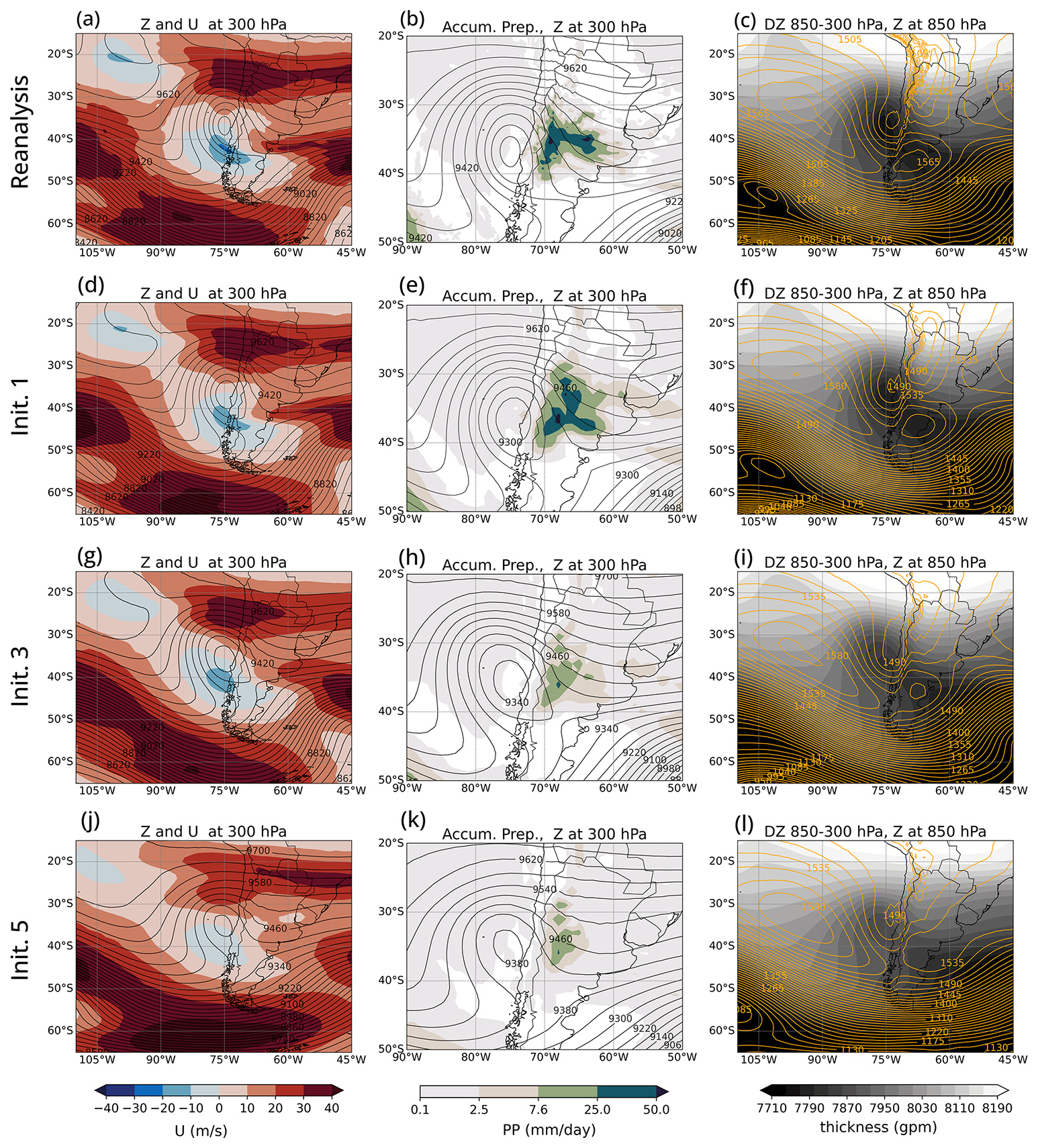
Figure 7 Segregation stage of the COL formed on 31 March 2013. (Top) ERA5 and (rows 2 to 4) GEFS predictions of (first column) geopotential height (Z; solid black lines, contour interval 40 gpm) and wind (U; shaded) at 300 hPa, (second column) geopotential height (Z; solid black lines, contour interval 40 gpm) at 300 hPa and accumulated precipitation (Accum. Prep.; shaded) over 24 h, and (right column) geopotential height (Z; solid orange lines, contour interval 20 gpm) at 850 hPa alongside the 300–850 hPa layer thickness (DZ; shaded). GEFS predictions correspond to init 1 (second row), init 3 (third row) and init 5 (fourth row), initialized on 30, 28 and 26 March 2013, respectively.

Forecast-wise, it is found that the location of the COL formation was accurately predicted 1 and 3 d ahead and even 5 d ahead, with a bias of less than 200 km northwest of its observed position (init 1, init 3 and init 5; second, third and fourth rows in Fig. 7). However, these initializations underestimated its intensity by −6, −11 and −14 gpm m⁻² in init 1, init 3 and init 5, respectively. The GEFS model accurately predicted the strength and extent of the strong upper-level winds associated with the COL (split-jet structure) and the upstream ridge of the COL for init 1, init 3 and init 5 (Fig. 7d, g, j). Particularly, during init 5 (Fig. 7j) it better predicted the intensity of the jet streak on the polar side of COL than the jet on the equatorial side. At mid-levels, the model successfully captured the cold core during init 1 and init 3, although with slightly less strength compared to ERA5 reanalysis. However, it failed to capture the cold core during init 5. Additionally, the cyclonic circulation at lower levels was displaced to the north relative to the observation (Fig. 7c, f, i), leading to the COL and lower-level cyclones being out of phase. This results in a different vertical structure in the forecasts with regard to the observations, which is consistent with the underestimation of the COL intensity in the model. As discussed by Pinheiro et al. (2021), the intensity of the COL directly affects its vertical structure. In this case, the incorrect forecast position of the cyclone at low levels likely weakened the upward vertical motion and low-level moisture convergence, both of which are key factors for precipitation development. This implies weaker vertical coupling in the forecast, resulting from the discrepancy in the intensity of the COL. Regarding precipitation forecasts, GEFS performs well in predicting the location of precipitation associated with COLs (with a slightly southeast bias), but it underestimates the amount of precipitation, especially during init 3 and init 5, with underestimations around 20 mm d⁻¹ (Fig. 7h, k).

3.3.2 Case study 2: COL development on 9 March 2019

On 9 March 2019, another COL formed off the coast of Chile, at 33° S, 74° W (first row of Fig. 8). This system was weaker than the one described in case 1 and lasted 4 d. It caused some weak precipitation in south-central South America, but the amounts were lower than those associated with the first COL.

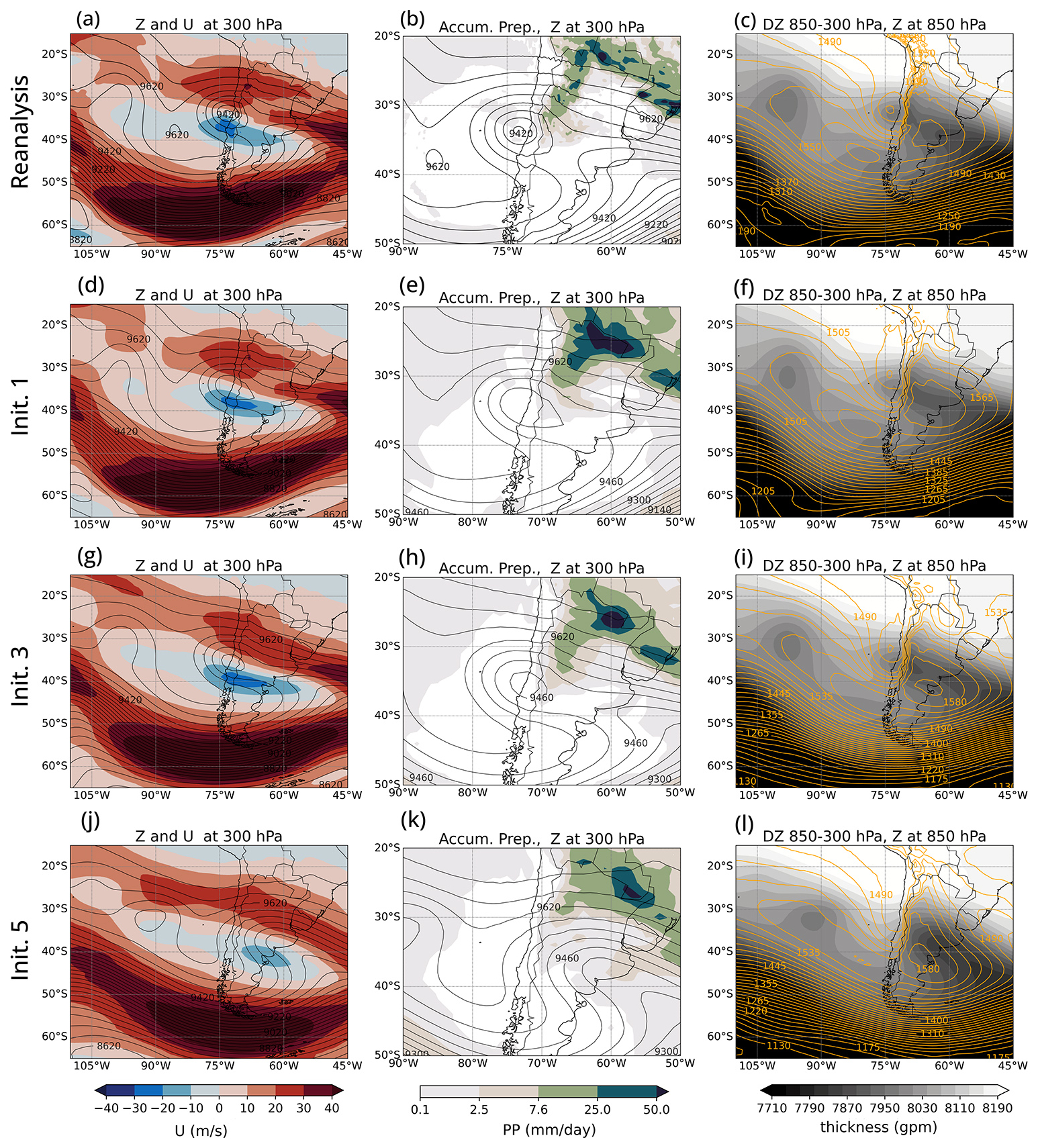
Figure 8 As in Fig. 7 but for the COL formed on 9 March 2019. In this case, the GEFS predictions corresponding to init 1 (second row), init 3 (third row) and init 5 (fourth row) were initialized on 8, 6 and 4 March 2019, respectively.

The synoptic environment during the segregation stage of this COL in the ERA5 reanalysis (first row of Fig. 8) included an upper-level ridge with a NW–SE axis to the southwest of the COL, a split-jet structure, a strong low-level cyclone positioned just beneath the COL center off the coast of Chile and a small cold core at middle levels. Although this COL had a smaller structure than the first COL, the cyclonic system extended into the lower levels, as evidenced by the accompanying low-level cyclone identified in Fig. 8c. In the precipitation field, two distinct maxima were identified: one located northeast of the analysis domain, associated with a decaying frontal zone in that area, which is linked to a surface cyclone positioned over the South Atlantic Ocean (not shown), and another maximum over western Argentina, directly related to the ascent zone east of the COL. The frontal system mentioned here is separated from the COL and its associated dynamics. The subsequent validation of the GEFS forecast focuses only on this second feature as it was the one directly associated with (or triggered by) the COL.

The GEFS forecasts for 9 March 2019 initialized 1, 3 and 5 d ahead are shown in Fig. 8 (second to fourth rows). Forecasts showed that the predicted position and intensity of the COL were consistently inaccurate across the three initializations. The COL was predicted to be shallower and displaced to the southeast, the system was shifted approximately 210 and 430 km from its observed location for init 1 and init 3, and it could not even be captured in init 5. Meanwhile, the intensity was underestimated by approximately 15 to 17 gpm m⁻². With respect to the upper-level winds associated with the COL, the GEFS demonstrated a good skill in forecasting both their intensity and their spatial positioning, particularly in relation to jet streaks on the polar flank of the COL. However, the model exhibited notable challenges in accurately representing the cold-core structure at mid-levels, with a complete absence of this feature in init 5. At lower levels, the representation of the closed cyclone at 850 hPa was similarly problematic, with the system being consistently displaced northwards and exhibiting weaker intensity than observations, especially in init 3 and init 5. In terms of precipitation, GEFS underestimated rainfall amounts in all initializations and was not able to represent the observed precipitation on the lee side of the Andes Mountains (Fig. 8e, h, k), displacing the predicted precipitation northeast of the observed location, particularly over central and northeastern Argentina. However, while the GEFS model generally underestimated rainfall amounts across all initializations, it is important to note that this behavior is expected given the model's relatively coarse resolution (1×1°), especially on the lee side of the Andes where the complex features of COLs usually make the simulation of precipitation difficult even in high-resolution regional models like WRF (Yáñez-Morroni et al., 2018).

Based on these results, a wrongly positioned and less intense COL can lead to a poor forecast of the vertical structure of the two case studies, including their cold core and associated low-level circulation, subsequently affecting dynamical processes such as horizontal temperature advection, thermodynamic instability, vorticity advection and associated ascent, which are ingredients for precipitation production downstream. Such errors may be related to the inadequate representation of diabatic effects or interaction with the Andes Cordillera (Garreaud and Fuenzalida, 2007). Even though the characterization of such processes is beyond the scope of this study, they will be addressed in future work.

4 Discussion and conclusions

This study explored the prediction skill of cut-off lows (COLs) in the NCEP Global Ensemble Forecast System (GEFS) with a focus on the region with the highest frequency of COL occurrence in South America during austral autumn (March to May). The analysis made use of a verification framework centered on the individual systems. These were identified and tracked using a feature-based approach applied to the 300 hPa level geopotential height as the primary variable.

The main conclusions can be built on the questions posed in the Introduction of the paper:

• What is the temporal scale at which GEFS can reliably predict the initiation phase of COLs, and how precise are these forecasts?

  The GEFS model is highly accurate in predicting the start of the segregation stage of COLs up to 3 d in advance, but this accuracy drops significantly as the lead time increases beyond 4 d. The percentage of COLs detected by the model decreases to 56 % and 29 % for predictions initialized 4 and 7 d ahead of the segregation, respectively. Our analysis also revealed that COL centers diverge by an approximate distance of 200 km relative to the observations up to 3 d in advance. However, this error increases to 600 km for forecasts more than 4 d ahead. Also, it has been shown that forecasts initialized up to 2 d in advance have no directional deviations, while forecasts initialized at least 3 d ahead of COL formation have a southerly bias. At the same time, the intensity errors show a consistent increase in magnitude, with values ranging from −2.5 gpm m⁻² in init 1 to approximately −13.0 gpm m⁻² at higher lead times.

• After formation, can GEFS accurately predict the subsequent trajectories of the COLs?

  From our results, we can conclude that the GEFS model has variable skill when forecasting the trajectories of COLs. Overall, errors in position increase from 200 to 400 km in forecasts of 1 to 2 d lead time. Within this time period, trajectories tend to be slower in comparison to the observed behavior. Even though this pattern of errors is also found for longer lead times, errors in predictions 3 d ahead increase substantially, and skill beyond 4 d is dramatically reduced. We can conclude that the trajectories of COLs can be relatively well predicted with lead times of up to 3 d, and forecasts initialized beyond that threshold are significantly degraded and depict a poor representation of the actual paths. Intensity-wise, we found that GEFS forecasts are characterized by an increase in the magnitude of underestimation of COL intensity as the lead time increases.

• Can errors in COL forecasts impact those of precipitation further downstream?

  Our two case studies suggest that the predictive skill of COLs, particularly regarding their formation location, intensity and trajectory, can influence precipitation forecasts downstream. In particular, the errors in the location and depth of the COLs appear to be linked to the mechanism sustaining these systems. In our case studies, the strength of the COL cold core could affect the thermodynamic instability patterns, potentially influencing vertical motion and precipitation formation downstream, even though further research would be needed to assess the actual role of the mechanisms at play. This is also further supported by the well-documented relationship between COL cold cores and atmospheric instability response (Pinheiro et al., 2021; Hirota et al., 2016; Nieto et al., 2007; Porcù et al., 2007; Llasat et al., 2007; Palmén and Newton, 1969), through which the dynamical ascent and atmospheric instability associated with the cold core trigger and/or enhance precipitation events (Godoy et al., 2011a; Nieto et al., 2007). Moreover, incorrectly forecasting the position of a low-level cyclonic system in association with COLs can significantly impact the vertical coupling of COLs, potentially influencing their intensity. This aligns well with Pinheiro et al. (2021), who suggested a possible relation between the intensity of COLs in South America and their vertical depth. These deficiencies, transferred into the higher levels, are able to shape the intensity of the system and, via this alteration, some of the mechanisms responsible for precipitation formation. As such, a weaker (stronger) COL will foster more (less) vorticity advection, resulting in favored (unfavored) ascent downstream. Therefore, predicted precipitation amounts will naturally be modulated by these errors (e.g., Saucedo, 2010). It should be noted, however, that these conclusions are driven by two case studies, and more research dealing with the processes associated with COL formation is needed.

Results from this study can be compared with similar recent studies. For instance, Lupo et al. (2023) have concluded that the operational GFS model has a systematic bias to move Southern Hemisphere troughs and COLs too quickly downstream, even though in our study region the identified bias is towards the west. (i.e., slower than observed). It should be noted, however, that the GEFS and the operational GFS share some common components but are different models, particularly regarding the horizontal resolution. As such, results from both studies are not directly comparable.

Regarding the case studies, previous authors analyzing the synoptic evolution and predictive skill of COLs in other regions of the world, such as Portmann et al. (2020) and Muofhe et al. (2020), have concluded that a proper representation of the COL's vertical structure is crucial for an accurate prediction of these systems. Pinheiro et al. (2021) also argue that the intensity of the COLs affect the entire structure of these systems and that errors in their intensity/position can easily affect their associated precipitation fields.

Although a detailed investigation of the physical mechanisms underlying these forecast errors was beyond the scope of this study, this issue is of great scientific importance for understanding the challenges typically found in predicting COLs. In this context, the GEFS bias, such as the westward bias and underestimation of intensity, likely arises from the model's inadequate representation of eddy–mean flow interactions, as explored by Nie et al. (2022, 2023) and Pinheiro et al. (2022). Moreover, in our study region, the positioning of the jet stream and the enhancement of transient wave activity over the South Pacific identified in previous work (GD12) are key to understanding these biases. Therefore, exploring the physical mechanisms underlying these forecast errors is essential. Future work exploring the simulation of jet streams and Rossby wave activity could provide crucial insights. Preliminary research has already shown that specific Rossby wave patterns preceding COLs can be predicted up to a week in advance, although confidence is reduced beyond that period (Choquehuanca et al., 2023).

It should be stressed once again that this study is proposed as a first step towards a full characterization of the physical processes responsible for COL formation, evolution and predictive skill in NWP systems. Several open questions remain, which will be addressed in future studies. Among them, it is unclear why the predicted trajectories are systematically slower than the observations. A negative correspondence between COL intensity and location was also observed in the GEFS dataset, suggesting that the most intense COLs seem to be associated with lower positional errors. However, the underlying mechanism sustaining such a relationship (if any) is not clear.

As a final note, future studies will dive into the relative contributions of COL intensity, location and speed on the resulting forecasted precipitation fields, as a deeper understanding of the interplay between these might bring useful information for operational weather predictions of high-impact events over southern South America.