On the movement of atmospheric blocking systems and the associated temperature responses

The quasi-stationary behaviour of atmospheric blocking is studied using a Lagrangian framework that enables the tracking of blocks in space and time. By combining a blocking index based on geopotential height with a Lagrangian tracking algorithm, we investigate the characteristics of atmospheric blocking events for different zonal velocities with respect to Earth's surface and their impacts on surface temperatures within the retuned EC-Earth3 global climate model. We observe that blocking events can portray a large variety of zonal velocities. Distinct differences are found between the behaviour of eastward-moving blocks and westward-moving blocks, both in size and in spatial distribution. Although the size of blocks is of bigger importance for the temperature anomalies, the zonal velocity has an influence on the strength of the temperature anomalies in winter, due to the slower mechanism of air advection in winter, compared to diabatic heating in summer. In summer, the zonal velocity primarily influences the positioning of temperature anomalies relative to the centre of the blocking system. These findings highlight the complex interactions between size, zonal velocity, and other blocking attributes, as well as their influence on temperature anomalies. Further research is warranted to explore regional differences in blocking behaviour and impact, as well as how atmospheric blocking and associated temperature anomalies may evolve under future climate conditions.

1 Introduction

Atmospheric blocking is a large-scale atmospheric process, where a persistent Rossby wave causes a strong high-pressure area to remain in place (Rex, 1950a, b; Platzman, 1968; Altenhoff et al., 2008). The influence of blocking events on our weather is significant as these blocks cover a large area, can last from days up to a month, and are quasi-stationary (Liu, 1994). Atmospheric blocking in winter is often associated with cold spells, which often form downstream of the block. Upstream of the block, a warm conveyor forms with warm air and moist conditions. Both these upstream and downstream processes are caused by horizontal advection of respectively warm air from the tropics and cold air from the polar regions, driven by the high-pressure area. In summer, heatwaves and droughts are often associated with persistent conditions of atmospheric blocking. During the day, diabatic warming and adiabatic warming due to subsidence reinforce each other and result in positive temperature anomalies (Bieli et al., 2015; Röthlisberger and Martius, 2019). As subsidence plays a bigger role in the realisation of higher temperatures in summer, these temperatures are found right underneath the block (Kautz et al., 2022).

The dynamics of atmospheric blocking have been a subject of research for over a century, predominantly due to the high-impact weather associated with them (Garriott, 1904). Since then, scientists have been trying to understand different blocking characteristics that contribute to the impact of blocks on our weather, such as their size (Nabizadeh et al., 2019), intensity (Wiedenmann et al., 2002; Davini et al., 2012), duration (Barnes et al., 2012), and location (Brunner et al., 2018; Sousa et al., 2017). Other topics that have been widely researched are the dynamics behind blocking formation and maintenance. Orography and land–sea contrasts have long been named as important contributors to blocking formation (Ji and Tibaldi, 1983). More recently, the release of latent heat during cloud formation has been evaluated by Pfahl et al. (2015), while Yamazaki and Itoh (2013) proposed the selective absorption mechanism as a contributor to the persistence of blocking.

An often overlooked aspect of atmospheric blocking is its geographic displacement during its lifetime. Because of its assumed quasi-stationary nature, this propagation is usually ignored for simplicity, and it is not explicitly included in often-used blocking indices (Sousa et al., 2021; Pelly and Hoskins, 2003). However, it can be argued that one of the primary reasons why atmospheric blocking is connected so strongly to high-impact weather is just because of its stationarity. Due to its stationarity, the associated anomalous low-pressure “bad-weather” sectors in its vicinity also remain locked in space, which could greatly amplify their destructive impacts. Sumner (1959) was the first to introduce the subject of blocking movement (or blocking propagation velocity), making the distinction between progressive (eastward-moving), quasi-stationary, and retrogressive (westward-moving) blocks. These categories were split by a threshold value of 5° per day in both the eastward and westward direction, and it was found that about 40 % of all blocks were quasi-stationary, 35 % were progressive, and 25 % were retrogressive for the Atlantic–European sector. However, as Sumner (1959) used a minimum blocking duration of 2 d, these values are probably not representative of our current understanding of blocks with a minimum duration of 4 d. These different blocking movement directions follow from the linear Rossby-wave theory:

$$\begin{array}{}\text{(1)}& c_{\mathrm{p}}={\displaystyle \frac{\mathit{\omega }}{k}}=U-{\displaystyle \frac{\mathit{\beta }}{k^{\mathrm{2}}+l^{\mathrm{2}}}},\end{array}$$

where c_p is the phase velocity, U is the mean westerly flow, β is the Rossby parameter, and k and l are the zonal and meridional wave number, respectively. While Rossby waves always retrogress with respect to the ambient mean flow U, Eq. (1) shows that, with respect to a (stationary) geographical location, the phase velocity becomes westward for larger/longer waves (i.e., small k and/or l) and eastward for smaller/shorter ones (Holton and Hakim, 2013). Recently, Luo et al. (2019) and Luo and Zhang (2020) have extended this into the nonlinear regime. Specifically, they show that in the nonlinear regime the blocking amplitude modifies the phase speed,

$$\begin{array}{}\text{(2)}& c_{N\mathrm{p}}=c_{\mathrm{p}}+c_N=U-{\displaystyle \frac{{\text{PV}}_y}{k^{\mathrm{2}}+l^{\mathrm{2}}+F}}-{\displaystyle \frac{{\mathit{\delta }}_N{M}_{\mathrm{0}}^{\mathrm{2}}}{\mathrm{2}k{\text{PV}}_y}},\end{array}$$

which is the sum of the phase velocity c_p and blocking-induced phase velocity c_N, with PV_y being the meridional background potential vorticity (PV) gradient, M₀ the maximum amplitude of the block, F≈1 the Froude number, and δ_N the nonlinearity strength defined in Luo et al. (2019). Around the same time, Mokhov and Timazhev (2019) showed the importance of blocking movement in blocking detection, since different threshold values of maximum zonal velocities led to different blocking frequencies. Lastly, Steinfeld et al. (2018) studied the distributions of the mean zonal velocity during the lifetime of blocks and concluded that this velocity was highest in their onset phase and decreased during their mature phase. They also mention that their blocking algorithm detected some blocks with velocities larger than 10 m s⁻¹ (864 km d⁻¹), but they doubted if they could be seen as classical blocks.

Within the realm of studies on blocking movement, studies on the effect of blocking movement on our weather have mostly been done on a local scale. For example, Chen and Luo (2017) showed that westward-moving Greenland blocking in winter results in larger cold anomalies in North America, while quasi-stationary Greenland blocking leads to colder anomalies in northern Europe and eastern Asia. Similarly, Yao et al. (2017) revealed that rapidly westward-moving Ural winter blocks lead to less persistent cold events over Europe combined with weak high-latitude warming, while slower westward-moving or quasi-stationary Ural winter blocks lead to strong cold anomalies over central and eastern Asia and stronger high-latitude warming. In our research, we will extend this knowledge by focusing on the full range of possible zonal velocities in the Northern Hemisphere and how they influence our weather in both summer and winter. For this analysis, we applied a Lagrangian perspective to the latest update of the climate model EC-Earth3_p5 (ECE3p5), which enables us to track a large number of blocks in space and time with respect to the Earth's surface, and we gather information on their individual characteristics. This method differs from the earlier-mentioned theoretical work done on blocking propagation velocities by Luo and Zhang (2020). Since we are interested in the associated impacts of the blocks at the surface, we use a surface-relative velocity instead of a theoretical propagation velocity of the blocks. This perspective offers a more dynamic view of blocks, enabling us to discern variations in zonal velocities and their corresponding influences on weather phenomena – a capability that remains elusive within an Eulerian framework. Our study has two main objectives: we will first assess the characteristics of the zonal velocity of atmospheric blocks and how they relate to blocking size, intensity, duration, and location; after that, we will look at the influence of the zonal velocity on temperature anomalies and compare this to the influence of blocking size to estimate the importance of the movement of atmospheric blocking.

2 Data and methods

2.1 The EC-Earth3_p5 model

In this study, we use simulations of the EC-Earth3_p5 climate model (ECE3p5), which is the latest update of EC-Earth3 (ECE3). One of the main shortcomings of ECE3 is its temperature bias compared to ERA5 reanalysis data. In the Northern Hemisphere, ECE3 has a cold bias, while in the Southern Hemisphere a warm bias dominates. Compared to ECE3, ECE3p5 has an even larger warm bias over the Southern Hemisphere but with a better representation of the temperature over the Northern Hemisphere (Muntjewerf et al., 2023; Van Dorland et al., 2023) (Appendix 5). As we are only evaluating the Northern Hemisphere atmospheric blocking, ECE3p5 is the most appropriate choice for this research. Later on, the ability of ECE3p5 to simulate atmospheric blocking is evaluated.

From ECE3p5, we use the historical dataset, which contains 16 ensemble members ranging from 1850 to 2014, resulting in a total dataset of 2624 years. These 16 ensemble members were created by perturbing the initial state of the system, thus giving rise to 16 climate realisations. The standard resolution is T255L91 (≈80 km) for the atmosphere, and the model uses time steps of 2700 s (45 min). For the sake of computation time and because of the large size and duration of atmospheric blocks, we regridded this dataset to a regular lat–long grid of 2.5° × 2.5° using bilinear interpolation, and we took the daily mean values. For the identification of the blocks, the geopotential height at 500 hPa (Z500) (m) is used. The other selected variable is the daily mean surface air temperature at 2 m (TAS) (K).

2.2 ERA5 reanalysis data

ERA5 reanalysis data are used to evaluate the ECE3p5 model. From this dataset, we only used the daily mean geopotential at 500 hPa (m² s⁻²) from 1950 to 2022, which is transformed to the geopotential height (hPa) (Copernicus Climate Change Service, 2023). ERA5 has a resolution of 0.25° × 0.25° (Hersbach et al., 2023), but to comply with our regridded ECE3p5 dataset, we regridded the 0.25° × 0.25° grid of ERA5 to 2.5° × 2.5°.

2.3 Blocking index

Since Rex (1950a) first introduced a definition of atmospheric blocking, multiple blocking indices have emerged to extract these blocks from datasets. They differ in the dynamical aspects of a block that they grasp but also in the minimal duration, size, or location of a block. Some indices only capture one-dimensional aspects, while others capture multiple dimensions. As a result, it is difficult to compare different studies on blocking events (Sousa et al., 2021; Davini and d’Andrea, 2020; Barnes et al., 2014).

The blocking index that we use here is based on the two-dimensional extension of the standard geopotential height index by Tibaldi and Molteni (1990) and takes the majority of alterations by Sousa et al. (2021) into account, which are meant to make the index more inclusive and precise. The first step in Sousa et al. (2021) is to exclude the subtropical high-pressure belt from the blocking analysis. While Sousa et al. (2021) use a daily mean value for the minimum latitude for all longitudes LAT_min (t), we chose to work with a longitude-dependent minimum latitude LAT_min (t, λ), which looks for the latitude at which the value of Z500 is higher than the Z500 value averaged over the previous 15 d:

$$\begin{array}{}\text{(3)}& Z\mathrm{500}(\mathit{\lambda },\mathit{\varphi },t)>\stackrel{\mathrm{‾}}{Z\mathrm{500}}.\end{array}$$

As the location of the subtropical high depends on the position of the sun and thus on the seasons, the minimum latitude is found further poleward in summer compared to winter. Especially over the wintertime European–Atlantic region, the choice of LAT_min makes a difference, since the longitude-dependent LAT_min (t, λ) is situated 7.5^∘ further poleward than LAT_min (t), which is shown in Fig. 1.

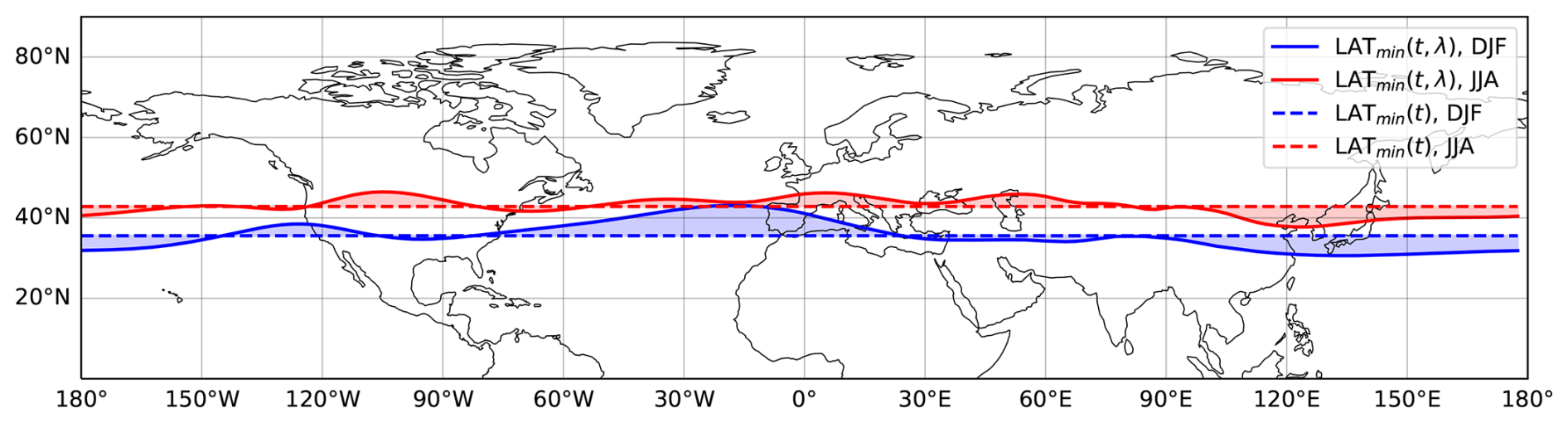
Figure 1 Difference between the latitude-dependent minimum latitude LAT_min (t,λ) (continuous line) and the spatially averaged minimum latitude LAT_min (t) (dashed line); both shown for winter (DJF, blue) and summer (JJA, red) for ERA5.

Above the minimum latitude, the blocks are filtered out using these geopotential height gradients (GHGs):

$$\begin{array}{}\text{(4)}& \begin{array}{rl}& \mathrm{\text{GHGS}}(\mathit{\lambda },\mathit{\varphi },t)={\displaystyle \frac{\left[Z\mathrm{500}\right(\mathit{\lambda },\mathit{\varphi },t)-Z\mathrm{500}(\mathit{\lambda },\mathit{\varphi }-\mathrm{\Delta }\mathit{\varphi },t\left)\right]}{\mathrm{\Delta }\mathit{\varphi }}}\\ & \text{if}{\mathrm{LAT}}_{\min }\le \mathit{\varphi },\end{array}\end{array}$$

$$\begin{array}{}\text{(5)}& \begin{array}{rl}& \mathrm{\text{GHGN}}(\mathit{\lambda },\mathit{\varphi },t)={\displaystyle \frac{\left[Z\mathrm{500}\right(\mathit{\lambda },\mathit{\varphi }+\mathrm{\Delta }\mathit{\varphi },t)-Z\mathrm{500}(\mathit{\lambda },\mathit{\varphi },t\left)\right]}{\mathrm{\Delta }\mathit{\varphi }}}\\ & \text{if}{\mathrm{LAT}}_{\min }\le \mathit{\varphi }\le \mathrm{75}\mathit{°},\end{array}\end{array}$$

$$\begin{array}{}\text{(6)}& \text{GHG}(\mathit{\lambda },\mathit{\varphi },t)=\sqrt{{\text{GHG}}_z^{\mathrm{2}+}{\text{GHG}}_m^{\mathrm{2}}},\end{array}$$

where we define the zonal gradient and the meridional gradient respectively as

$$\begin{array}{}\text{(7)}& {\text{GHG}}_z={\displaystyle \frac{Z\mathrm{500}(\mathit{\lambda },\mathit{\varphi }+\mathrm{\Delta }\mathit{\varphi },t)-Z\mathrm{500}(\mathit{\lambda },\mathit{\varphi }-\mathrm{\Delta }\mathit{\varphi },t)}{\mathrm{2}\mathrm{\Delta }\mathit{\varphi }}},\end{array}$$

$$\begin{array}{}\text{(8)}& {\text{GHG}}_m={\displaystyle \frac{Z\mathrm{500}(\mathit{\lambda }+\mathrm{\Delta }\mathit{\lambda },\mathit{\varphi },t)-Z\mathrm{500}(\mathit{\lambda }-\mathrm{\Delta }\mathit{\lambda },\mathit{\varphi },t)}{\mathrm{2}\mathrm{\Delta }\mathit{\lambda }}},\end{array}$$

with $\mathrm{\Delta }\mathit{\lambda }=\mathrm{\Delta }\mathit{\varphi }=\mathrm{2.5}$°. Following Sousa et al. (2021), a grid cell is said to be in a blocked state when GHGN < 0, GHGS > 0, and GHG $(\mathit{\lambda },\mathit{\varphi },t)<\mathrm{20}$ m per degree. Sousa et al. (2021) also limit the evaluation of GHGN at a latitude of 75°, above which blocked grid cells fall under the designation of polar blocks. Since these polar blocks differ in character from the general blocking definition, they are excluded in this analysis. Furthermore, blocks are excluded whenever their maximum size is smaller than 5×10⁵ km² and their total lifespan (duration) is shorter than 4 d, with no differentiation made among various block types as is done by Sousa et al. (2021). Lastly, we apply the method of Wiedenmann et al. (2002), which was modified by Davini et al. (2012) to be two dimensional, to derive a quantification of blocking intensity (BI) indicative of the strength of the block:

$$\text{RC}(\mathit{\lambda },\mathit{\varphi },t)\equiv {\displaystyle \frac{\begin{array}{c}(Z_{\mathrm{u}}+Z\mathrm{500}(\mathit{\lambda },\mathit{\varphi },t\left)\right)/\mathrm{2}+\\ (Z_{\mathrm{d}}+Z\mathrm{500}(\mathit{\lambda },\mathit{\varphi },t\left)\right)/\mathrm{2}\end{array}}{\mathrm{2}}}$$

$$\begin{array}{}\text{(9)}& \mathrm{BI}(\mathit{\lambda },\mathit{\varphi },t)=\mathrm{100}\left[{\displaystyle \frac{Z\mathrm{500}(\mathit{\lambda },\mathit{\varphi },t)}{\mathrm{RC}}}-\mathrm{1.0}\right].\end{array}$$

In Eq. (9), RC stands for representative contour, and it is used to normalise the Z500 values. Z_u is the minimum Z500 value within 60° upstream of a grid cell with value Z500, and Z_d is the minimum Z500 value within 6° downstream of this same grid cell. The value resulting from it indicates how the meridional circulation is affected by the presence of the block, where Northern Hemisphere blocks are defined as weak when they have a value of BI < 2.0, moderate when 2.0 < BI < 4.3, and strong when BI > 4.3. Wiedenmann et al. (2002) based this categorisation on which blocks were within and outside of 1 standard deviation of the 30-year mean intensity of their dataset. Applying the described method leads to the climatological blocking intensities shown in Fig. 2, which can be compared to the results from the CMIP6 models in Davini and d’Andrea (2020). The blocking climatologies of ERA5 and ECE3p5 differ in their mean blocking intensity in certain regions, which are more prominent during the separate seasons than for the annual mean. An overestimation or underestimation can be caused both by an overestimation or underestimation of the number of blocks and by its intensity. Annually, ECE3p5 underestimates the BI over western Europe and Scandinavia and overestimates the BI over Alaska and Siberia. In winter, BI is generally higher than the annual mean, with two dipoles to be found in the comparison between the model and reanalysis data: one with underestimation over western Europe and overestimation over the Ural region, and one with an underestimation over the Bering Sea and an overestimation over Alaska. In summer, lower BI values are found, together with the same dipoles for the differences between ERA5 and ECE3p5 but switched in sign. These dipoles are further discussed in Sect. 4.1.

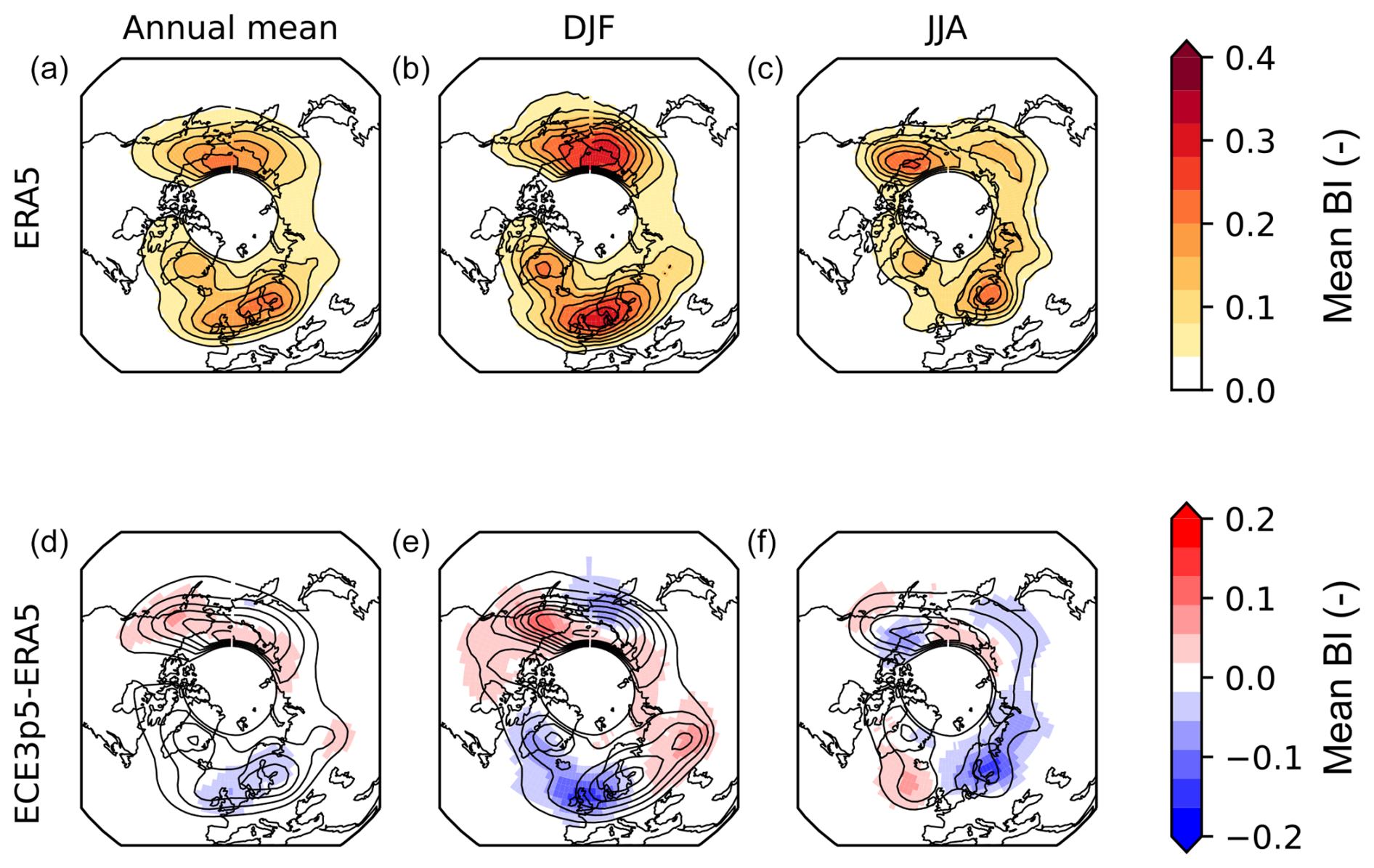
Figure 2 (a–c) Climatological blocking intensity of ERA5 (contours and shading) for the annual mean, winter mean (DJF), and summer mean (JJA). (d–f) Contours show blocking intensity of ECE3p5, and shading shows the difference between ERA5 and ECE3p5 for the annual mean, winter mean, and summer mean. The data from both ERA5 and ECE3p5 are taken over the period of 1951–2014.

2.4 2D cell-tracking algorithm

As we want to evaluate the movement of atmospheric blocks with respect to the Earth's surface, we work from a Lagrangian point of view. Using the 2D cell-tracking algorithm of Lochbihler et al. (2017), we can find continuous cells and track them in time. Continuous cells are formed from adjacent grid cells that meet our blocking index. Continuous cells belong to one track when there is overlap between the cells during consecutive time steps. The algorithm results in information on the total size per day, the lifespan (duration), both mean and maximum intensity per day, intensity-weighted centre per day, and dates of onset and decay. From this information, blocks are selected with a minimum duration of 4 d. The size of the blocks is converted from the number of grid cells to square kilometres (km²) using the latitude of the intensity-weighted centre as ϕ in

$$\begin{array}{}\text{(10)}& \mathrm{d}x\approx \mathrm{2}\mathit{\pi }R\cos \mathit{\varphi }{\displaystyle \frac{{\mathrm{2.5}}^{\circ }}{\mathrm{360}\mathit{°}}},\end{array}$$

where R is the radius of the Earth and 2.5° the size of our grid cells. After small and short-lived blocks are removed, the movement of the remaining blocks with respect to the Earth's surface is calculated. As the primary moving direction of the blocks is zonal, we only take the zonal velocity into account. This velocity is calculated by comparing the intensity-weighted centre of a block at its date of onset to its date of decay and by dividing this zonal distance in kilometres by the blocking duration. This method is consistent with the velocity used by Steinfeld et al. (2018). Blocks are categorised as winter or summer blocks based on their onset date respectively being in the months of DJF (December, January, or February) or JJA (June, July, or August). A summary of this complete method is showcased in Fig. 3a. As a proof of concept, the longitudes of the weighted centres for each day of the duration of an arbitrary block are plotted against the accompanying latitude-averaged Z500 anomalies and the blocking intensity in Fig. 3b and c, respectively. A more in-depth analysis of this can be found in Sect. S5 in the Supplement.

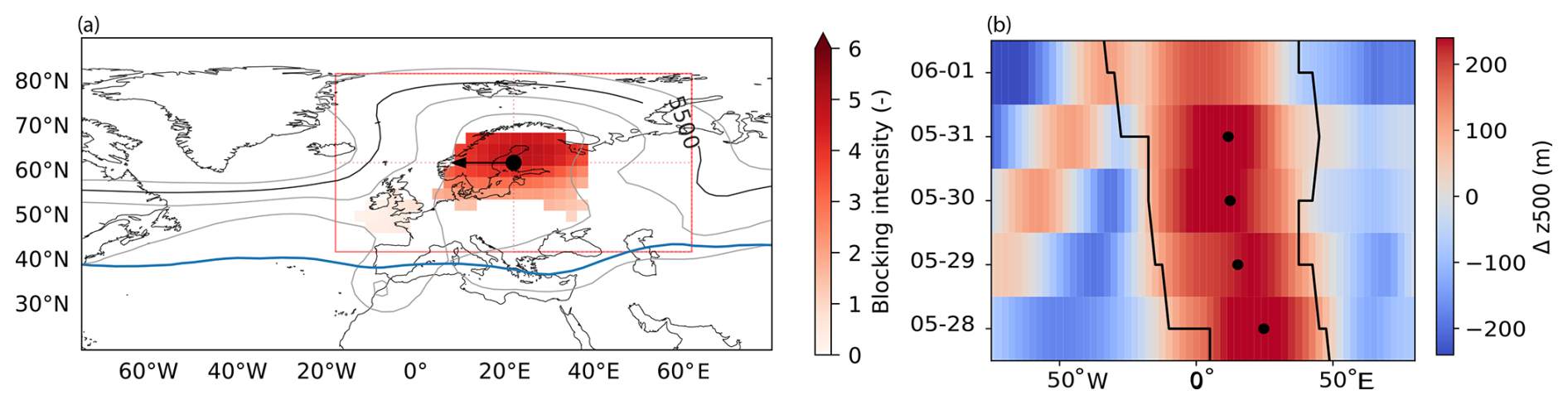
Figure 3 (a) Example of an atmospheric block (ERA5: 28 May 1963) filtered out by the method of Sousa et al. (2021) but with a variable minimum latitude (blue line) and added blocking intensity (red) (Wiedenmann et al., 2002), tracked by the cell-tracking algorithm. The black dot denotes the weighted centre of the block, and the arrow denotes the zonal velocity and direction. The contour lines show the geopotential height (Z500) for 5400, 5500 (black), 5600, and 5700 m. The red rectangle is the area used to evaluate the temperature, divided into four subareas. (b) A Hovmöller plot of the Z500 anomaly (m) over the duration of the same block as in (a), starting on 28 May 1963 and ending on 1 June 1963. Z500 is averaged around the latitude ±5° following from the weighted centre on the starting date of the block. The black dots denote the weighted centres of the block according to the cell-tracking algorithm. The black contour shows the boundaries of the block following from Eqs. (4), (5), (6), (7), and (8).

2.5 Impact on temperature

To assess the impact of different zonal velocities on our weather, we look at the daily mean surface air temperature at 2 m, detrended and corrected for climatology to get temperature anomalies. This is done by calculating the climatological daily mean per ensemble member and subtracting this mean from each day in the dataset. These temperature anomalies allow us to compare the impact of blocking on different locations and during different seasons. As blocks do not only influence the temperature right underneath the block but also in the areas around it, we work with a fixed area around the blocking centre. This area is set to have a latitude width of 40° and a longitude width of 80° (see red rectangle in Fig. 3). The size of this area is selected to encompass the size of the majority of the blocks, ensuring that it adequately captures the diverse range of temperature anomalies associated with them. This size is comparable with approximately a quarter of the area shown in Fig. 3. We divide the 40° × 80° area around the block into four quadrants to incorporate the different temperature anomalies upstream and downstream of a block. We only take into account those temperature anomalies that are measured over land, as the ocean has a significantly larger thermal warming capacity compared to land (Cess and Goldenberg, 1981). Consequently, it takes longer for the surface area underneath the block to warm or cool over the ocean. At the same time, the temperature effects of blocks are primarily experienced by us on land. Therefore, the land surface temperature anomalies are of particular relevance when considering the impacts of blocking events.

3 Results

3.1 Comparison between ERA5 and ECE3p5

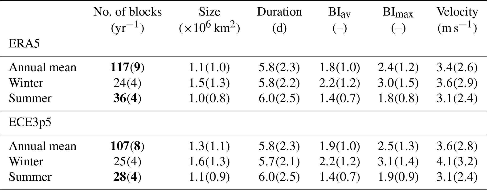
We evaluate the accuracy of ECE3p5 to simulate blocking behaviour by comparing the output of the tracking algorithm for ECE3p5 to the output for ERA5. This is done for the number of blocks per year, their average size, duration, average intensity, maximum intensity, and absolute velocity. This information is summarised in Table 1 for the annual and seasonal (winter/summer) values of blocks within ECE3p5 and ERA5 after aggregating over the entire Northern Hemisphere.

Variables that differ significantly between ERA5 and ECE3p5 according to the t test are shown in bold. Comparing all variables shows that the only significant differences can be found in the annual mean and summer mean number of blocks, where ECE3p5 simulates fewer blocks than can be observed in ERA5. From these values, it is likely that the difference in the annual mean, which has 10 more cases in ERA5, is caused by the difference in the summer mean, which has 7 more cases in ERA5. However, we can not exclude any contributions from spring and autumn, as these seasons are not taken into account. The difference between the number of summer and winter blocks is also larger for ERA5 than for ECE3p5. All other variables do not show significant differences, possibly due to the relatively large standard deviations, indicating the big differences between individual blocks. For both ERA5 and ECE3p5, winter blocks are generally larger, more intense, and reach higher absolute zonal velocities than summer blocks, while their durations are about the same. For the size and duration, it should be noted that our minimum requirement was respectively 5×10⁵ km² and 4 d, as described in Sect. 2.3. Not shown in Table 1 is the direction of the velocities, which can be both eastward and westward, as we only show the absolute velocity here. However, we found the annual mean direction to be positive, meaning that on average atmospheric blocks are moving towards the east, although with lower velocities than the typical synoptic wind speed of 10 m s⁻¹, which is likely a representation of the background flow (kernel density estimation (KDE) distributions in Fig. 4, direction of P10–90 blocks in Fig. S5). All these characteristics align with the findings of Cheung et al. (2013), who found similar differences between winter and summer for the number of blocking events and their intensity, as well as comparable numbers for the duration and a general eastward-moving trend. This same eastward trend was also observed in a case study by Steinfeld et al. (2020) using potential vorticity (PV) anomalies and by Hirt et al. (2018) using a point vortex model but not yet on this scale for all observed blocks in reanalysis and model data.

Table 1 Blocking statistics over the period of 1951–2014 for ERA5 (above) and ECE3p5 (below). Significant differences between ERA5 and ECE3p5 are shown in bold. Numbers in the table denote the mean and standard deviation. The standard deviation is taken over all blocks within the specified season over all 16 ensemble members. The velocity is the absolute zonal velocity of the blocks.

3.2 Relation between zonal velocity and other characteristics

Table 1 only results in seasonal averages per blocking characteristic. We extend this analysis to all winter and summer blocks separately, which allows us to study any correlations between the different blocking characteristics and the zonal velocity. In Fig. 4, the zonal velocity is plotted against the average size, duration, and average intensity over the total duration of the block, for both summer and winter. Next to the kernel density estimation (KDE, in shading), the 10th, 50th, and 90th percentiles of respectively average size, duration, and average intensity are used to mimic the behaviour of the two extreme states and the mean state of the characteristics per velocity bin of ≈0.5 m s⁻¹. Moving towards more extreme velocities, the results get noisier due to the few numbers of cases. Alternative versions of this figure of different longitudinal sections of the world can be found in the Supplement (Figs. S12 and S13).

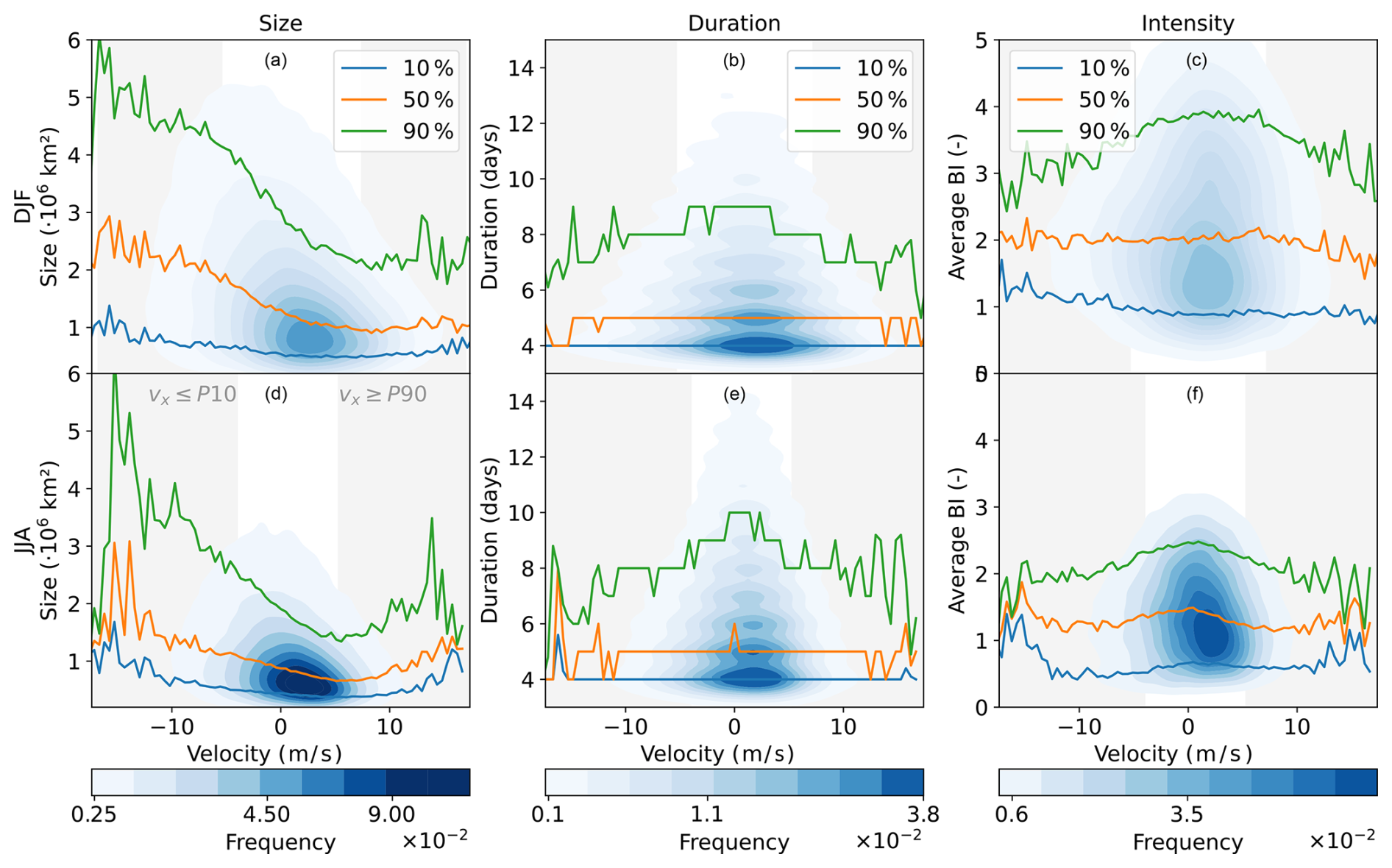
Figure 4 Kernel density estimation (blue shading, linear) and the 10th (blue), 50th (orange), and 90th (green) percentiles for the average size (a, d), total duration (b, e), and average intensity (c, f), all for winter (DJF, a–c) and summer (JJA, d–f). Taken from 1850 to 2014 over all 16 ensembles of ECE3p5. In the background, grey shading shows where the zonal velocity is smaller than the 10th (winter: $\le -\mathrm{3.0}$ ms⁻¹; summer: $\le -\mathrm{2.0}$ ms⁻¹) or larger than the 90th (winter: ≥5.1 ms⁻¹; summer: ≥4.0 ms⁻¹) velocity percentiles, representing respectively westward- and eastward-moving blocks.

The size is shown in the first column of Fig. 4. From the KDE, it is noticeable that the blocking size is much more confined to smaller sizes in summer, while the spread is larger in winter. The majority of the blocks in both winter and summer are on the smaller side compared to the total spread and are associated with eastward velocities. On the contrary, the largest blocking sizes are associated with westward velocities. This uneven allocation becomes even clearer when looking at the percentiles, which represent the 10 % smallest, the 10 % largest, and the median blocking size per velocity bin. It is consistently observed across both seasons that the larger the block, the faster it moves westward. Towards the quasi-stationary blocks, the blocking size decreases. In winter, the blocking size stays approximately the same for different eastward velocities, while in summer the blocking size slightly increases again. This result is similar to the propagation of Rossby waves according to linear Rossby-wave theory, described in Eq. (1), and the nonlinear theoretical phase speed in Eq. (2), where a large amplitude will act to enhance the retrogression, just as is seen in Fig. 4.

The duration of the blocks is plotted against the zonal velocity in the second column of Fig. 4. The KDE and the percentiles for the duration are not as smooth compared to those for size or intensity. This disparity arises from the discrete nature of duration measurements, quantified in whole days, in contrast to the continuous values of size and intensity. The KDE is pyramidal for both winter and summer, with the longest durations over the stationary blocks. In both seasons, blocks with shorter durations occur more frequently than blocks with longer durations. The 90th percentile shows for both winter and summer that stationary blocks have a longer duration than the faster-propagating blocks. The 50th percentile, which shows the mean value per bin, is 5 d for almost all velocities and therefore does not show the same relationship as the 90th percentile line. The 10th percentile is a straight line at 4 d, which is the minimum duration threshold that we set in Sect. 2.3.

The final blocking characteristic that is compared to the zonal velocity is the average blocking intensity in the third column. The first notable difference between winter and summer is the spread in the data, as shown by the KDE. The winter months exhibit a much larger variability and higher values than the summer months. Both seasons display an oval distribution around slightly eastward-moving velocities, with a denser core for lower intensities. This indicates that the more stationary blocks display the largest range in blocking intensities. For the percentiles in winter, only the 90th percentile shows this same relationship of larger intensities for quasi-stationary blocks. The 50th and 10th percentiles do not show this, and stay around the same BI no matter the velocity, which can also be deduced from the broader base of the KDE. In summer, the 90th percentile shows a larger BI for quasi-stationary blocks and lower strengths for faster-moving blocks in both directions, although combined with a lot of noise at the outer boundaries. The variation in the 50th and 10th percentiles is minimal, just as for winter. This shows that the stronger intensities do counteract the general westerly background flow, as can also be seen in Eq. (2) where M₀ counteracts U but only as much as to result in a stationary block. For lower intensities, this effect can not be seen in Fig. 4.

Combining all the information in Fig. 4 tells us that quasi-stationary blocks are generally smaller, have a longer duration, and have a broad variation in strength; the 10 % fastest eastward-moving blocks are generally larger than quasi-stationary blocks, have a shorter duration, and a smaller variation in strengths; lastly, the 10 % fastest westward-moving blocks are bigger than both quasi-stationary and eastward-moving blocks, are of shorter duration, and have a smaller range of strengths than quasi-stationary blocks. This is in line with the theoretical results of Zhang and Luo (2020), who found that a smaller meridional basic potential vorticity gradient favours westward-moving blocks with larger size and higher intensity and vice versa for larger meridional potential vorticity gradients.

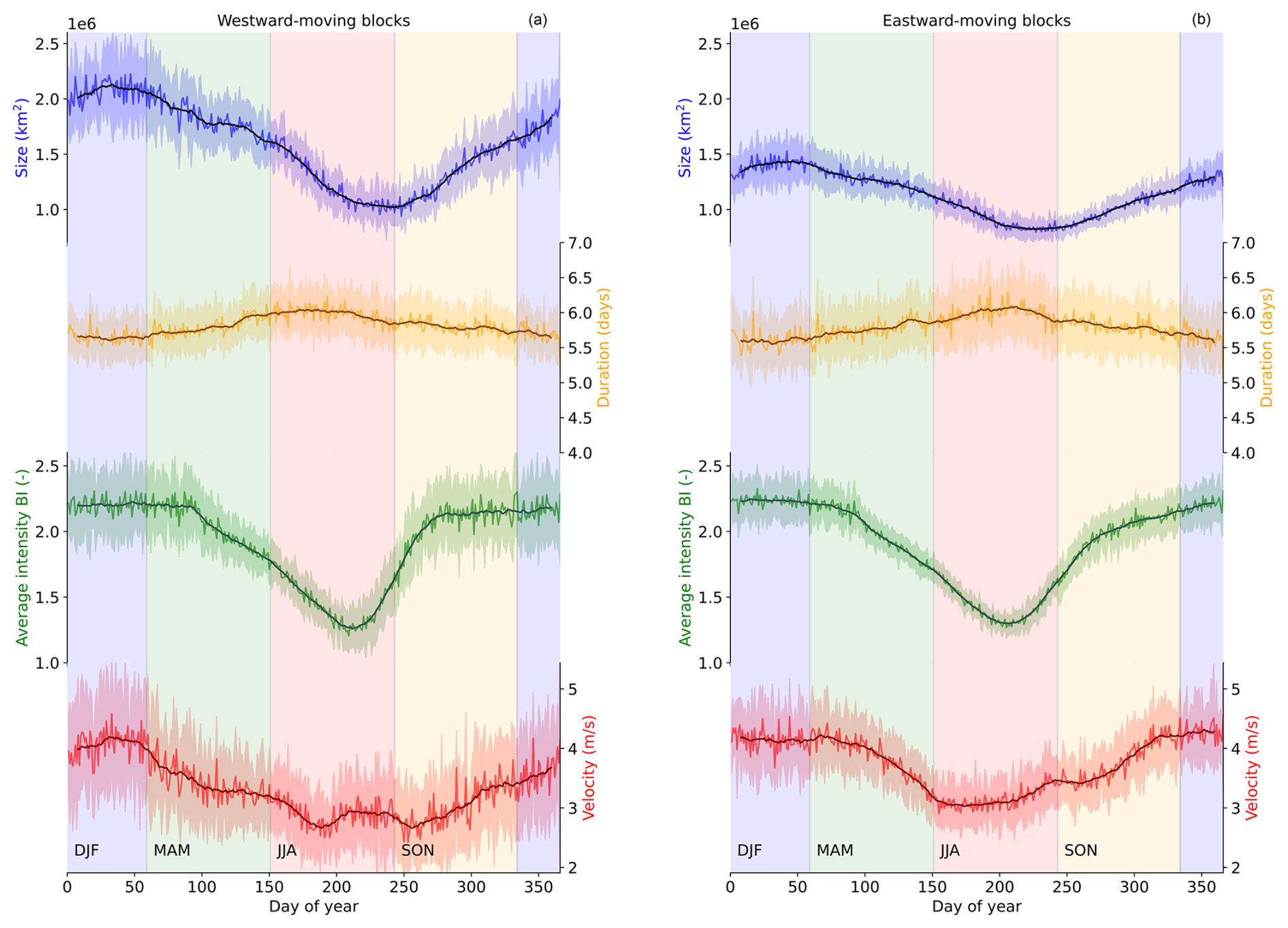
Figure 5 Blocking characteristics for (a) westward- and (b) eastward-moving blocks. The characteristics shown are the mean size (blue), the duration (yellow), the average intensity (green), and the absolute zonal velocity (red) over the years of 1850–2014 and all 16 ensembles of ECE3p5. The darker lines are the 15 d rolling means, and the lighter lines show the mean values over all blocks and ensembles per day of the year. The shading is the standard deviation of the 16 ensemble members.

3.3 Seasonality of westward- and eastward-moving blocks

Westward-moving blocks and eastward-moving blocks thus seem to behave differently, especially when it comes to their size. To extend our analysis of the different aspects of blocking behaviour further, we assess the seasonality of westward- and eastward-moving blocks separately. This is done in Fig. 5 for the average size, duration, average intensity, and absolute velocity per day of the year, with all westward-moving blocks (v_x<0) on the left and all eastward-moving blocks (v_x>0) on the right. Note that the velocity is absolute (positive) for both eastward and westward blocks and thus represents the amplitude and not the direction of the velocity.

The zonal blocking velocity (red in Fig. 5) is the first variable to be examined and later compared to the other variables. Both the eastward and the westward velocities have a seasonal cycle with higher values in winter, a decrease in velocity in spring, a minimum in summer, and an increase in velocity again in autumn. Notably, there are discernible differences between the two. On average, eastward-moving blocks tend to have higher velocities than their westward counterparts across all seasons. However, these disparities diminish during the transition from spring to summer and towards the end of winter. Both have their maximum velocities in winter, with a value of 4.3±0.5 m s⁻¹ for the eastward blocks and 4.2±0.5 m s⁻¹ for the westward blocks, where the velocity and its variability are respectively the mean and 1 standard deviation over all ensemble members and years on that specific day of the year. The eastward-moving blocks have their maximum at the end of December, while the westward-moving blocks have their maximum at the beginning of February. However, as the eastward-moving blocks have roughly the same velocity throughout the whole winter, this maximum is more spread out than for the westward-moving blocks. Their minimum velocities also differ, as the eastward velocities have their lowest values in June (3.0±0.5 m s⁻¹), while the westward velocities have their lowest values in July and September (2.7±0.5 m s⁻¹). Over the year, both blocking types thus exhibit roughly the same seasonality but with shifts in their minima and maxima of one to 2 months, combined with larger values for eastward-moving blocks.

After the division of all atmospheric blocks over westward-moving and eastward-moving blocks, the other blocking characteristics are also split up according to their zonal direction, leading to different sizes (blue), durations (yellow), and intensities (green) for the westward-moving blocks in Fig. 5a and the eastward-moving blocks in Fig. 5b. When we split up the size of the blocks with respect to their direction of movement, a clear distinction arises between the size of the blocks that move to the west and those that move to the east. Over the seasons, westward-moving blocks are consistently larger than eastward-moving blocks, with the disparities being more pronounced in winter compared to summer. Both have their maximum size at the end of winter, with values of $\mathrm{1.4}\pm \mathrm{0.2}\times {\mathrm{10}}^{\mathrm{6}}$ km² for the eastward variant and $\mathrm{2.1}\pm \mathrm{0.4}\times {\mathrm{10}}^{\mathrm{6}}$ km² for the westward variant. Their minimum size is found at the end of summer, with values of $\mathrm{0.8}\pm \mathrm{0.2}\times {\mathrm{10}}^{\mathrm{6}}$ km² for the east and $\mathrm{1.0}\pm \mathrm{0.4}\times {\mathrm{10}}^{\mathrm{6}}$ km² for the west. Apart from the differences in size, there are no clear differences in the seasonality between the two blocking directions. This leads to an interesting misalignment or lag of 2 months between the minimum velocity and the minimum size for eastward-propagating blocks, while the minimum size of the westward-propagating blocks can be found more in the middle of its velocity minima.

The next variable is the duration of the blocks. As indicated in Table 1, the variations across seasons are minimal. A similar observation holds true for the two blocking directions, where only marginal differences exist among the two. Both the eastward and westward blocks have the same values for their minima and maxima, with a minimum value of 5.6±0.2 d and a maximum value of 6.1±0.2 d. This results in a difference of 0.5±0.2 d between the minima and the maxima of the blocks. Within these small differences, both blocking directions have their maximum duration in July and their minimum in winter.

The final variable is the average blocking intensity, which reveals a distinct seasonality that is approximately consistent for blocks moving in both directions. Both have a constant average intensity over the winter and parts of spring and autumn, which then rapidly declines in summer. The only difference seems to be that the transition between the steady state in winter and the minimum value in summer is more abrupt for the westward-moving blocks compared to the eastward-moving blocks. Both have minimum values of 1.3±0.3 in July and maximum values of respectively 2.3±0.3 and 2.2±0.3 in winter for eastward and westward blocks. Over the year, the average intensity is higher during seasons when blocks also have a higher velocity and lower in seasons with lower velocities.

3.4 Spatial distribution of different blocking velocities

Categorising blocks into velocity-based groups leads to further insights into the different behaviours of the fastest westward- and eastward-moving blocks. When ordering the zonal velocities from negative to positive, a division is made between the first 10 % (v_x≤P10), which are the fastest westward-moving blocks, and the last 10 % (v_x≥P90), which are the fastest eastward-moving blocks, as well as all blocks in between ($P\mathrm{10}<v_x<P\mathrm{90}$). For each group, the coordinates of the weighted centres of the blocks based on their BI on the fourth day of their existence are used to show where the different groups of blocks occur most. The choice of the fourth day aligns with the division made by Steinfeld et al. (2018) between the onset phase (days 1 and 2) and mature phase (days 3, 4, and 5) of the block. By focusing on the fourth day, we ensure that we assess the blocks during their mature phase, although it can be seen in Fig. S5 that the blocks continue to move over the whole lifespan. This analysis was performed for both winter and summer, resulting in Fig. 6. It is important to note that the 10 % fastest eastward- and westward-moving blocks do not have the same velocities in winter and summer, as is evident from the distinct distributions in Fig. 4. These values are $P\mathrm{10}=-\mathrm{3.0}$ m s⁻¹ and P90=5.1 m s⁻¹ for winter and $P\mathrm{10}=-\mathrm{2.0}$ m s⁻¹ and P90=4.0 m s⁻¹ for summer. Additionally, it should be kept in mind that the distribution shown in Fig. 6 is only a representation of the centres of the blocks and not their entire spatial extent.

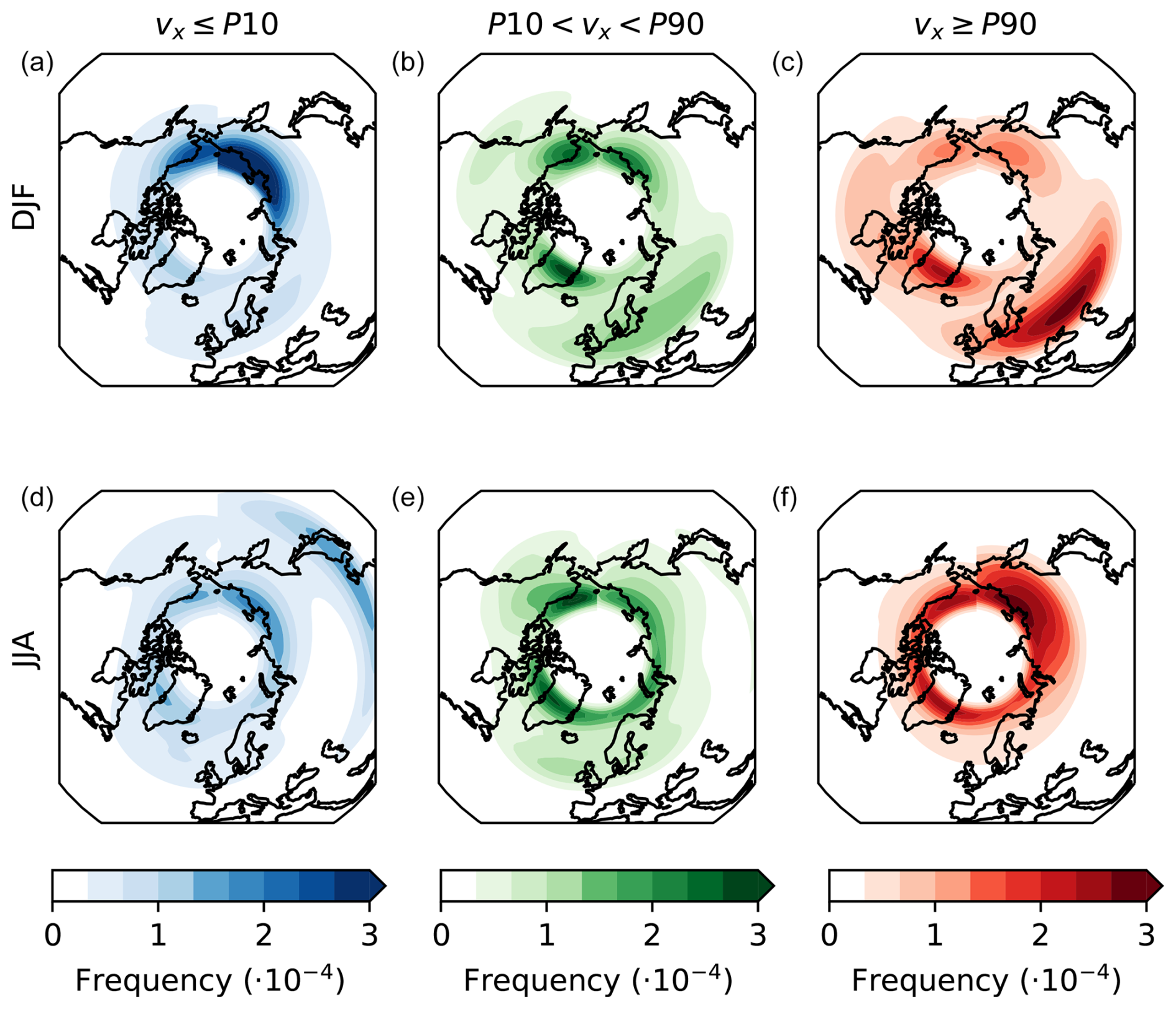
Figure 6 Spatial-distribution-weighted (based on BI) blocking centres, on the fourth day, with (a, d) the 10 % fastest westward-moving blocks (v_x≤P10), (b, e) all zonal velocities in between ($P\mathrm{10}<v_x<P\mathrm{90}$), and (c, f) the 10 % fastest eastward-moving blocks (v_x≥P90), all taken separately over all winter months (DJF, upper row) and over all summer months (JJA, lower row) over the period of 1850–2014 for all 16 ensembles of ECE3p5.

The spatial distribution differs per group of blocks. The majority of the blocks are represented by the $P\mathrm{10}<v_x<P\mathrm{90}$ group (middle column). In winter, these blocks are most commonly found over Greenland, Alaska, and northeast Siberia, and in lower numbers stretching from western Europe into Russia. Comparing this spatial pattern to the 10 % fastest westward-moving blocks (v_x≤P10, first column), we can see that the hotspot over Europe is now less present and shifted north. Greenland is also less featured for the P10 blocks, while especially the hotspot over northeast Siberia has a much higher frequency compared to the average blocking pattern. The 10 % fastest eastward-moving blocks (v_x≥P90, third column) show the exact opposite tendency. The hotspots over Alaska and northeast Siberia are a little less featured for the P90 blocks, while the pattern over Europe has intensified and also shifted southeastward. The hotspot over Greenland shows the same pattern of frequency for the P90 blocks as the average spatial pattern. Overall, we can say that northeast Siberia is the preferred location for faster westward-moving blocks, while faster eastward-moving blocks are more commonly found over middle Eurasia.

The spatial distribution of summer blocks is quite different from the winter distribution. As the middle column for the $P\mathrm{10}<v_x<P\mathrm{90}$ blocks shows, summer blocks are usually more confined to the higher latitudes, which we expect to be the case due to a combination of factors, such as the absence of a mean jet during summer, combined with the shifting minimum latitude of the high-pressure belt with the seasons, and the exclusion of polar blocks by the maximum latitude. In summer, Rex blocks are common over the North Pole, and it is possible that we see the remnants of those blocks here (Sousa et al., 2021). Higher frequencies are found over Greenland and Alaska, although blocks are quite evenly distributed between those areas. P10 blocks occur more often over Siberia than over Alaska and Greenland, similar to the winter circumstances. The spatial pattern of the P10 blocks deviates from the mean at lower latitudes in Asia, which seems to be just above our minimum latitude. These could consist of anomalously large ridges moving towards the west, which might still be captured by our blocking index. The P90 blocks, on the other hand, resemble the mean blocking pattern quite closely. There is a strong confinement to the higher latitudes, with an even distribution between the North Sea and the Bering Sea. The highest frequencies are found over Siberia, which is also the region with the largest deviations compared to the mean situation. Although the differences are smaller in summer compared to winter, it is clear from Fig. 6 that blocks that have different zonal velocities also reside in different areas. The underlying mechanisms for this observation remain to be studied.

3.5 Influence of the velocity on temperature

Within the examining of the relationship between various blocking characteristics and the zonal velocity, Fig. 4 revealed that quasi-stationary blocks tend to have longer durations and higher intensities, making them more likely to have a significant impact on our weather. On the contrary, the fastest westward-moving blocks exhibited larger surface areas, while quasi-stationary blocks were generally smaller in size. Considering that both larger and more stationary blocks are expected to contribute to higher-temperature anomalies, it is important to determine the respective contributions of these factors. First, we compare temperature anomalies with different zonal velocities; subsequently, we assess the impact of blocking size compared to velocity on temperature anomalies.

To investigate whether the velocity affects the temperature anomalies resulting from the block, we look at the results for the lower-right quadrant (see Sect. 2.5) in Fig. 7. The other quadrants can be found in Figs. S9, S10, and S11. As the quadrants mostly differ in the strength of the anomalies but not so much in the patterns related to the velocities, we choose to discuss just one of them here.

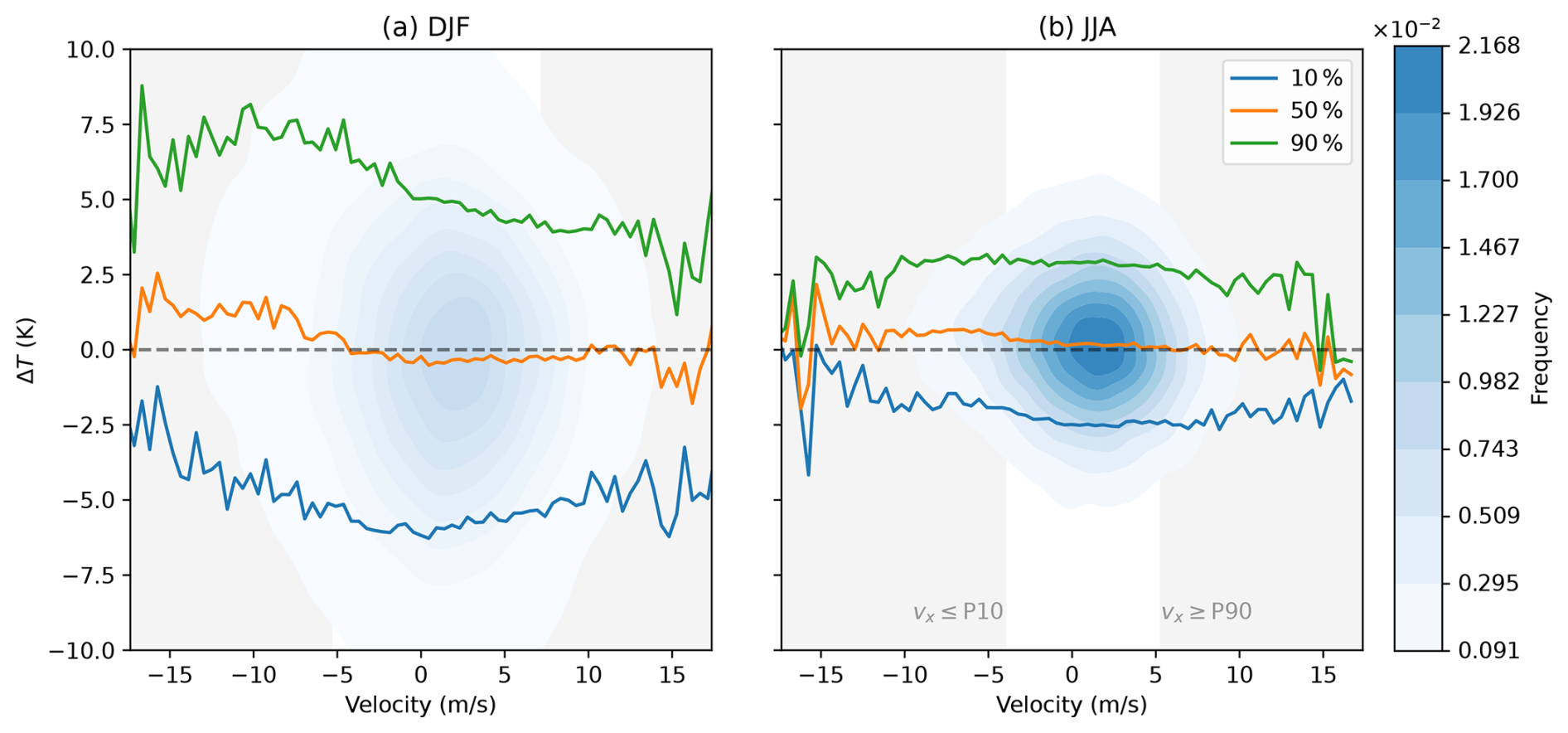
Figure 7 Kernel density estimation (blue shading) and the 10th (blue), 50th (orange), and 90th (green) percentiles of the lower-right quadrant of the 2 m temperature anomaly plotted against the zonal velocity, all for winter (DJF, a) and summer (JJA, b). Only temperature anomalies over land are taken into account, taken over the period of 1950–2014 over all 16 ensemble members of ECE3p5; grey shading for P10 and P90 is the same as in Fig. 4.

The temperature anomalies over land are plotted against the zonal velocities in Fig. 7 for winter and summer. In the KDE plot in winter, a broad range of temperature anomalies is observed, ranging from −10 to 10 °C. The majority of blocks result in relatively small temperature anomalies, as is indicated by the 50th percentile, which is around zero degrees for most velocities. This is in line with our earlier results in Fig. 4, where it was shown that the majority of the blocks are relatively small, of short duration, and relatively weak. These blocks result in lower-temperature anomalies, moderating the mean values. Simultaneously, the coldest temperature anomalies are also measured for stationary blocks, indicating a correlation between lower temperatures and stationary blocking conditions. This result is in line with the research done by Brunner et al. (2017), who showed that cold spells take longer to develop due to the slow process of horizontal advection of cold air. Conversely, the warmest temperature anomalies can be associated with the faster westward-moving blocks, which creates an interesting contrast between the blocking velocities associated with the coldest temperatures. The pattern of the warmest 10 % temperature anomalies looks similar to the relation between size and velocity in Fig. 4, so possibly the larger block size associated with faster westward-moving blocks plays a role in these larger temperature anomalies. Although winter blocks are mostly related to cold spells, this figure clearly demonstrates that these winter blocks can generate a wide range of temperature anomalies (not limited to negative values).

In contrast to the winter conditions, the temperature anomaly differences in summer exhibit a more constrained distribution. The KDE plot displays smaller excesses, the 50th percentile remains about zero, and the 10 % warmest and coldest temperature anomalies are just a little higher than ±2.5 °C. Notably, none of the percentiles exhibit a discernible trend, as their values remain relatively consistent across the entire range of zonal velocities, with just a little smaller anomalies towards the extreme velocities, although clouded by the noise in the signal. The insensitivity of the temperature anomalies with respect to the velocities can be attributed to the different warming processes in summer, caused by both diabatic and adiabatic warming, both faster processes than air advection such that the warming effect can still take place beneath faster-moving blocks. Especially for Rex blocks, this warming underneath the block goes hand in hand with cooling underneath the accompanying lower-pressure area to the south of the block. These lower temperatures are represented by the 10 % lowest temperature anomalies in Fig. 7. The relatively small temperature anomalies observed in summer compared to winter can be attributed to multiple factors. Firstly, the data used for this analysis consists of daily mean temperatures. The cloud-free conditions that cause warming underneath these summer blocks during the day also cause cooling during the night. These lower night temperatures moderate the overall daily mean values. To quantify this effect, it would be necessary to study the differences in response between the minimum and maximum temperatures. Secondly, as argued by Cheung et al. (2013), the continent is already warmer in summer, leading to lower-temperature anomalies. Additionally, pressure gradients are smaller in summer compared to winter. This last argument can be compared to the blocking intensity that we studied in Fig. 5, where indeed summer blocks generally exhibit lower blocking intensities compared to winter blocks.

In order to assess the different effects of the zonal velocity and size on temperature anomalies, a composite analysis is performed in which all blocks are divided according to their size and velocity. This result is shown in Fig. 8 for temperature anomalies measured over land. On the x axis, the velocities are sorted from the largest negative (westward) values (0 %) to the largest positive (eastward) values (100 %), showing the most extreme velocities per 5 % and the quasi-stationary blocks between 10 %–90 %. The y axis shows the size per 20 %, from small (0 %) to large (100 %). For both winter and summer, the quasi-stationary blocks with a velocity closest to zero are found at roughly 40 % (see Table 2). The choice to use percentiles and not absolute differences in size or velocity was made to ensure that every composite mean has enough cases for a reliable result. As a consequence, the percentiles do not represent the same velocity or size values for winter and summer, as the percentages are taken separately for the two seasons. The values that the percentages represent are shown in Table 2.

Table 2 Blocking sizes and zonal velocities for different percentiles in winter and summer, used in Fig. 8, based on ECE3p5.

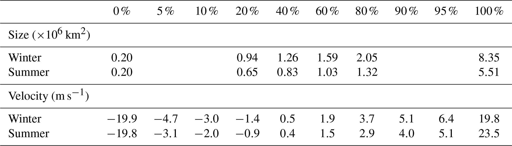
Figure 8 shows the composite mean analysis for winter (a) and summer (b) over land. Focusing on winter, it is evident that for every combination of size and zonal velocity, a distinct pattern emerges for temperature and Z500. Positive temperature anomalies are consistently observed to the northwest of the block, while negative temperature anomalies are observed to the southeast of the block. For all of them, the positive temperature anomalies dominate in value over the negative temperature anomalies. When we compare blocks with different sizes for the same velocity, the temperature anomalies become stronger and take over a larger part of the selected area around the block, just as the block itself grows. This result is to be expected, as a larger block will influence the temperature over a larger area. Comparing blocks with different velocities but with the same size reveals a change in the temperature and Z500 pattern. In the case of westward-moving blocks, the surface area surrounding the block exhibits a larger proportion of positive temperature anomalies, primarily concentrated to the north of the block, extending towards the westward-tilted blocking centre. The faster eastward that a block moves, the more confined the positive temperature anomalies are to the northwest, leaving more room for the negative temperature anomalies.

For summer in Fig. 8b, the dipole structure typical for Rex blocks is clearly visible. Each combination of size and velocity has a warm core around the centre of the block and a cold core to its south. Just as in winter, the temperature anomalies get stronger for larger blocks, although this seems to primarily affect the warm core. The cold cores are stronger for the quasi-stationary and eastward-moving blocks. For the same size but different velocities, the temperature anomaly pattern barely changes, which is what we expected based on the faster warming mechanisms in summer. The only notable change is a zonal shift of the dipole with respect to the blocking centre, combined with a tilt of the Z500 lines in the same direction as the movement of the block. For westward-moving blocks, the warm core is located on the east side of the blocking centre, while for the fastest eastward-moving blocks the warm core is located more on the west side of the block. Not only the location of the dipole as a whole changes, but it also tilts more towards the east for westward-moving blocks and towards the west for eastward-moving blocks. For both directions, the warm core is thus located on the upstream side of the block as a result of the warming that has already taken place there.

4 Discussion on methodology

4.1 Model biases

The results in Sect. 3 need to be considered in light of the model accuracy and choices that were made for the blocking index. In Sect. 2.1, it was described that the ECE3p5 model was chosen as it simulates more realistic temperatures for the Northern Hemisphere compared to ECE3. In Fig. S1b, the warming trend in both ERA5 and ECE3p5 can be seen for the Northern Hemisphere, where the warming trend in ECE3p5 is stronger than for ERA5. However, this trend does not seem to significantly change the model outputs for the velocity of atmospheric blocks over the years, as can be seen in Fig. S6. Therefore, the differences in temperature trends are probably of minimal importance for the velocity, although they may be important for other blocking characteristics (Woollings et al., 2018; Nabizadeh et al., 2019). At the same time, a positive temperature anomaly caused by a block will affect us more in a warmer climate, which makes for a new research topic on the impacts of blocks under global warming.

Temperature is also closely linked to the geopotential height anomalies. Higher temperatures lead to an expansion of the lower atmosphere and thus to a higher anomaly in geopotential height (Christidis and Stott, 2015). This relation between temperature and geopotential height anomaly is evident in both the model and the reanalysis data, as depicted in Fig. S2, but with an overestimation of the geopotential height anomaly of ECE3p5. In addition to this overestimation, the model also tends to overestimate its gradients, as indicated in Fig. S3, where the regions of underestimation are identical to the regions where the model underestimates the blocking frequency in Fig. 2. The correlation between the overestimation of Z500 and the blocking frequency is less prominent, but can still be recognised. These findings suggest that the model's biases in Z500 and its gradients may contribute to its limitations in accurately representing blocking events.

Other biases that play a role in most climate models are overestimation of the jets over the oceans (Anstey et al., 2013; Delcambre et al., 2013; Pithan et al., 2016) and misrepresentation of the orography (Narinesingh et al., 2020; Berckmans et al., 2013). Although we did not test if those biases are also incorporated into the ECE3p5 model, it is plausible to think so. Models often simulate jets to be too strong and too far inland. As blocks form at the end of those jets, this results in an eastward shift of the blocking frequency in models. This same effect can be seen for the winter simulations of ECE3p5 in Fig. 2, where the model underestimates the number of blocks over the Atlantic and the Pacific, while there is an overestimation over Russia and Alaska. The orography plays an important role in mountainous areas, such as the Ural and Alaska. These regions both show a negative bias in the number of simulated blocks by ECE3p5.

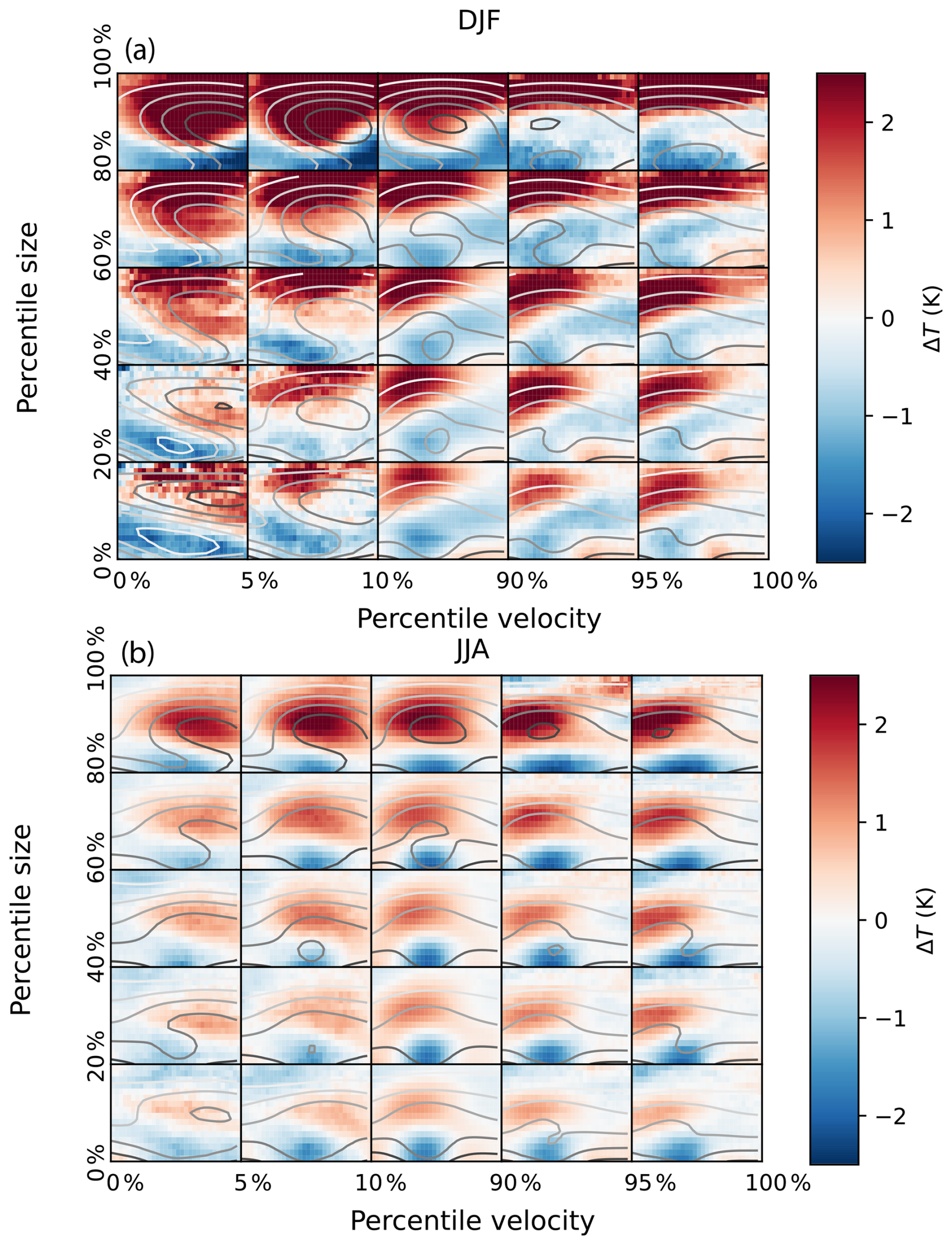
Figure 8 Composite mean of 2 m temperature anomalies over the duration of each block, in a region of 40° × 80° around the blocking centre over land. The winter season (DJF) is shown in (a), and the summer season (JJA) is shown in (b). On the y axis, the size is divided by its percentiles, going from small to large. On the x axis, the zonal velocity is divided by its percentiles, going from negative values to positive values. The division between westward-moving blocks and eastward-moving blocks is indicated by the arrows. In grey contours, the Z500 field is shown, with darker colours indicating higher Z500 values. Data are taken from ECE3p5 from 1850 to 2014 and over all 16 ensemble members.

4.2 Choice of blocking index

As discussed in Sect. 2.3, there are many different blocking indices used by researchers. These differences in the definition and calculation of blocking indices can have implications for the outcomes of our study. Here, we examine some of these discrepancies and how they may affect our results.

One significant modification we made compared to the method proposed by Sousa et al. (2021) was the redefinition of the minimum blocking latitude, as depicted in Fig. 1. This adjustment of the minimum blocking latitude resulted in a mean poleward shift of the minimum latitude over the Atlantic and a mean equatorward shift over the Pacific Ocean. These shifts have implications for the identification and measurement of blocking events. When we use a fixed minimum latitude, we get the blocking frequency as shown in Fig. S7, where indeed more ridges are captured than in Fig. 2. Consequently, this divergence also impacts the outcomes presented in Fig. 6. Using the more static minimum latitude of Sousa et al. (2021) leads to Fig. S8. In this figure, the blocks appear to be concentrated along the minimum latitude, particularly during the summer season. This shows the extent to which our results are influenced by the chosen minimum blocking latitude.

Some studies employ a second geopotential height gradient to further refine the selection of blocking events. This additional gradient,

$$\begin{array}{}\text{(11)}& {\text{GHGS}}_{\mathrm{2}}(\mathit{\lambda },\mathit{\varphi },d)={\displaystyle \frac{\begin{array}{c}\left[Z\mathrm{500}\right(\mathit{\lambda },\mathit{\varphi }-\mathrm{\Delta }\mathit{\varphi },d)-\\ Z\mathrm{500}(\mathit{\lambda },\mathit{\varphi }-\mathrm{2}\mathrm{\Delta }\mathit{\varphi },d)]\end{array}}{\mathrm{\Delta }\mathit{\varphi }}},\end{array}$$

is also used by Sousa et al. (2021), but they use it solely to differentiate between Rex blocks and omega blocks. Keeping the additional gradient would thus lead to a loss of all blocks that do not have the strong flow reversal underneath the block, such as omega blocks and ridges. This additional gradient is also used by Davini and d’Andrea (2020). The results that Davini and d’Andrea (2020) get for their blocking frequencies resemble our result in Fig. 2, even though they used a fixed minimum latitude of 30° N. Their use of GHGS₂, which restricts their blocks mostly to Rex blocks that are found at higher latitudes, presumably allows for the use of a lower and fixed minimum latitude.

A last important aspect of our study is the utilisation of blocking centres, which are tracked using the 2D cell-tracking algorithm. As outlined in Sect. 2.4, the blocking centre is determined by weighting the blocking intensity. Considering our minimum blocking area of 500 000 km², the blocking centre has the potential to move a considerable distance while remaining within the boundaries of the blocked area. Despite this, we opted to work with the weighted centre rather than an unweighted centre due to the association of higher intensities with greater impacts. As some of the blocks had long tails with a very low intensity, the unweighted centre would have trailed too far away from the area that is impacted by the blocks.

4.3 Other simplifications

Our study involves more simplifications that may impact the analysis and results. One notable simplification is the treatment of all blocks as equal events, despite their spatial variations, as demonstrated in Fig. 6. Blocks occurring at different locations can lead to varying impacts due to factors such as orography, orientation to large water bodies, and latitude, all of which can influence the temperature and humidity of the advected air. While we attempt to compensate for this simplification by separating blocks over land and over oceans, a lot of detail will be lost due to the generalisation.

Another simplification we made was to focus on winter and summer months. This decision is based on the distinct characteristics of blocks during these seasons, and they are also the most studied in the literature. However, it is important to recognise that even within these seasons there are variations that are averaged out when analysing on a seasonal basis, as illustrated in Fig. 5. The transitional character of spring and autumn makes these seasons more of a challenge to assess. As Brunner et al. (2017) found, the average relation between blocks and their temperature impacts changes during spring, which makes it even more interesting for research in a warming world.

Lastly, the choice to work with a Lagrangian framework for studying the temperature influences of blocking events is not immediately intuitive, especially not when you are interested in the weather directly overhead. However, this approach does offer valuable new insights into how blocking events lead to different temperature anomalies and which factors contribute to them. It also reveals that the impact of a block is not confined solely to the region directly underneath stationary blocks, as faster-moving blocks leave a trace of temperature anomalies as well. Generally, we can thus expect a faster-moving block to impact any region that it will cross in the near future. To obtain a more comprehensive picture, it would be beneficial to project the Lagrangian temperature profiles to specific areas of interest. This would enable a better understanding of how blocks, whether they are slowly travelling or stationary, influence temperature patterns in specific regions. By integrating the local-scale projections, we would be able to use both the advantages of a Lagrangian framework and the practical implications for local weather conditions.

5 Conclusions

In conclusion, this study aims to advance our understanding of the movement of atmospheric blocking and its influence on temperature anomalies at the Earth's surface. Atmospheric blocking has been extensively studied since the 1950s (Rex, 1950a), with a lot of focus on its frequency and impact on our weather in different seasons (Kautz et al., 2022). However, the velocity of atmospheric blocking has been fewer in number, primarily due to the general quasi-stationary nature of blocks and the predominant use of an Eulerian framework in their analysis. Previous studies that did consider the velocity treated it as a secondary aspect, without delving into its significance (Sumner, 1959; Steinfeld et al., 2018; Mokhov and Timazhev, 2019) or looking at local effects in specific blocking locations (Chen and Luo, 2017; Yao et al., 2017). Steinfeld et al. (2018) concluded their study on blocking propagation by mentioning that some blocks portrayed larger velocities of 10 m s⁻¹ (864 km d⁻¹) but that perhaps they could not be seen as classical blocks.

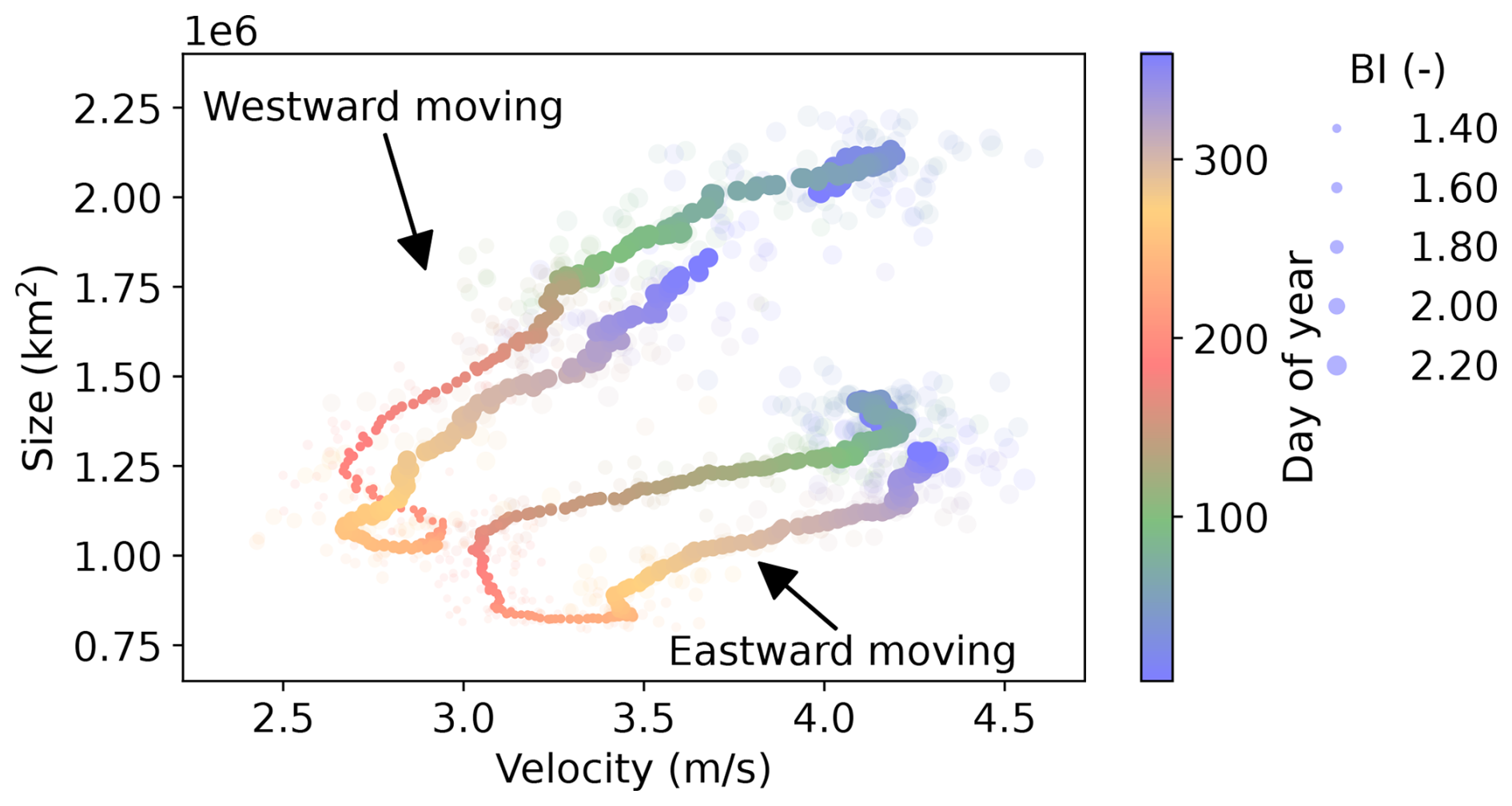
Figure 9 Climatological values per day of the year for size (km²) against absolute values of the zonal velocity (m s⁻¹). The scatter size indicates the blocking intensity (–), and the colour indicates the day of the year. Each day of the year is averaged over the period of 1850–2014 over all 16 ensembles (light colours) of ECE3p5, and a 15 d running mean is plotted (opaque colours).

To address this research gap, this study adopts a Lagrangian perspective to gain deeper insights into the dynamics of atmospheric blocks. By combining the blocking index of Sousa et al. (2021), the blocking intensity of Wiedenmann et al. (2002), and the cell-tracking algorithm of Lochbihler et al. (2017), together with some alternations where needed, we employ a unique methodology to identify and track the blocks. With this combination of methods, we evaluate the performance of the EC-Earth3_p5 climate model compared to ERA5 reanalysis data, examine the seasonality of the zonal velocity and its interplay with other blocking attributes, and investigate the influence of the velocity on temperature anomalies in comparison to blocking size.

The evaluation of the model performance reveals differences in the spatial distribution of blocking frequency and intensity between ERA5 and ECE3p5. Especially in summer, ECE3p5 underestimates the numbers of blocks over large regions in the Northern Hemisphere, such as over Scandinavia, Alaska, and parts of Russia. This underestimation over Europe is a well-known limitation of climate models (Woollings et al., 2018). However, when considering frequency, size, duration, intensity, and zonal velocity collectively, the only significant difference between ERA5 and ECE3p5 was observed in the summer frequency.

After the evaluation of the ECE3p5 model, we examined the characteristics of atmospheric blocks, focused on their seasonality, and explored relationships between different blocking aspects. Although quasi-stationary blocking events make up the majority of the blocks, our findings reveal a wide range of possible velocities, spanning values from −17.5 to +17.5 m s⁻¹, as determined by our blocking index. These values surpass those reported by Steinfeld et al. (2018), who questioned the classification of blocks exhibiting similar velocities. Additionally, we identify seasonality in the size, duration, blocking intensity, and velocity, with duration showing the least pronounced seasonal variation and the others exhibiting clearer patterns. The size, intensity, and velocity exhibit their minimum values in summer, albeit with some phase shifts among them, while the duration reached its maximum during this season. These results align with the differences between summer and winter blocks found by Cheung et al. (2013).

Another noteworthy discovery is the disparity in behaviour between eastward-moving blocks and westward-moving blocks, which is summarised in Fig. 9. On a seasonal basis, westward-moving blocks display larger sizes and a more linear relationship between size and velocity compared to eastward-moving blocks. The observed relationship resembles Rossby-wave theory, wherein the largest blocks are associated with westward velocities, while smaller blocks tend to exhibit eastward velocities. In contrast, the duration and intensity have their maxima for quasi-stationary blocks. Furthermore, we find that the fastest westward-moving and eastward-moving blocks occupied distinct locations compared to the majority of the blocks, and these locations also varied across seasons. In winter, the fastest eastward-moving blocks are predominantly found over Greenland and stretching from eastern Europe to Russia, while in summer they are located over Siberia. The fastest westward-moving blocks are situated over Siberia in both winter and summer.

Investigating the influence of the zonal velocity on surface temperature anomalies, temperature anomalies are found to be larger in winter than in summer. This could partly be attributed to the use of daily mean temperatures, which are tempered in summer due to lower values during cloud-free nights, and to the already warmer continent in summer, leading to smaller anomalies. In winter, the coldest temperatures are associated with quasi-stationary blocks, while the warmest temperatures are associated with westward-moving blocks. This same relation was also found by Zhang and Luo (2020), who showed that westward-moving Greenland blocks were related to lower concentrations of sea ice in winter. On the contrary, no clear relations are found during the summer. This can be explained by the different warming and cooling mechanisms in winter and summer, which are slower in winter and thus require more time to create larger temperature anomalies, while their effect is almost immediate in summer. We find that even the faster zonal velocities contribute to temperature anomalies.

Upon categorising the blocks according to their size and velocity, we observe distinct temperature patterns during winter and summer. In winter, the composite mean of all blocks exhibits warmer temperature anomalies to the northwest of the block and colder temperature anomalies to the southeast. In summer, the composite mean reveals warmer temperature anomalies beneath the block and colder temperature anomalies to its south. Comparing these patterns to the mean state of the blocks, we find that larger blocks induced more-intense temperature anomalies, while smaller blocks resulted in less pronounced temperature anomalies. The zonal velocity plays a role in determining the temperature anomaly patterns. In winter, faster eastward-moving blocks lead to more confined warm anomalies, and faster westward-moving blocks lead to a larger spread of warm anomalies. In summer, the size has the same effect as in winter, but the velocity only influences the location of the warm and cold anomalies relative to the block. Temperature anomalies for faster eastward-moving blocks are situated to the left of the block, while for faster westward-moving blocks they appear to the right. In both cases, the largest temperature anomalies are observed upstream of the block, where the block already had the opportunity to warm the surface area below it.

Answering the question about whether or not the fastest-moving systems can still be considered as blocks is hard. Following the blocking definition used here based on the general Z500 blocking index, these systems are filtered out as blocks. Additionally, we found that they result in temperature impacts similar to stationary blocks. However, the influence of these systems on stationary locations on Earth might be different due to their faster passing times, such that they may not be experienced as a classical block there. For future work, it would therefore be interesting to investigate this subject further on a more localised scale to discern regional differences more effectively. Questions on why certain types of blocks are more confined to specific regions than others also remain to be investigated. Additionally, exploring how the velocity may change under global warming and its potential implications for temperature anomalies would be of great interest. Understanding these dynamics could enhance our understanding of the evolving impacts of atmospheric blocking in a changing climate.