Weather type reconstruction using machine learning approaches

Weather types are used to characterise large-scale synoptic weather patterns over a region. Long-standing records of weather types hold important information about day-to-day variability and changes in atmospheric circulation and the associated effects on the surface. However, most weather type reconstructions are restricted in their temporal extent and suffer from methodological limitations. In our study, we assess various machine learning approaches for station-based weather type reconstruction over Europe based on the nine-class cluster analysis of principal components (CAP9) weather type classification. With a common feedforward neural network performing best in this model comparison, we reconstruct a daily CAP9 weather type series back to 1728. This new reconstruction constitutes the longest daily weather type series available. Detailed validation shows considerably better performance compared to previous statistical approaches and good agreement with the reference series for various climatological analyses. Our approach may serve as a guide for other weather type classifications.

1 Introduction

Weather type (WT) or circulation type classifications are a widely used tool to characterise the prevailing large-scale synoptic weather patterns over a specific region (Philipp et al., 2010). In regions such as Europe, where daily weather is largely governed by transient high- and low-pressure systems, such classifications prove particularly useful to describe the prevailing atmospheric conditions. WT time series yield important information about variability and changes in atmospheric patterns (Jones et al., 2014; Rohrer et al., 2017; Kučerová et al., 2017) and the surface effects associated with them (Paegle, 1974; O'Hare and Sweeney, 1993; Kostopoulou and Jones, 2007; Lorenzo et al., 2008; Jones and Lister, 2009; Casado et al., 2010; Küttel et al., 2011). Various studies have assessed the links between WTs and extreme events such as droughts (Fleig et al., 2010), temperature extremes (Hoy et al., 2020; Sýkorová and Huth, 2020), or extreme precipitation and floods (Minářová et al., 2017; Petrow et al., 2009). Moreover, WT classifications are applied to evaluate weather forecast model outputs (Stryhal and Huth, 2019; Weusthoff, 2011) or for forecasting in the renewable energy sector (Wang et al., 2022; Drücke et al., 2021; Li et al., 2020), among other uses.

The first WT classifications were created by experienced meteorologists, who classified the atmospheric situation, employing manually drawn weather charts derived from station observations (Hess and Brezowsky, 1952; Lamb, 1972; Schüepp, 1979). While these subjective classifications represent real synoptic features, they are often subject to inconsistencies and ambiguities (e.g. James, 2007; Cahynová and Huth, 2009; Jones et al., 2014; Wanner et al., 2000). In more recent decades, hybrid (mixed) or objective (automatised) WT classifications have been introduced that classify atmospheric patterns numerically using various statistical approaches, such as clustering algorithms, class attribution based on a distance measure, or even machine learning approaches (Huth et al., 2008; Mittermeier et al., 2022). Such automatised WT classification is usually based on gridded meteorological data (Huth et al., 2008). Because the temporal coverage of such gridded datasets is limited, WT classifications usually only reach back several decades. By creating long-term time series of WT classifications, important information may be gained to study long-term changes (i.e. over multiple decades or even centuries) in atmospheric circulation patterns and associated surface effects.

Based on reanalysis datasets, many WT records have already been extended back to the 19th century and some even back to the late 19th century (Philipp et al., 2010; Jones et al., 2014). The latest generation of reanalyses would allow these to be extended even further back in time. Currently, the limit for WT classifications based on atmospheric fields is set by the 20th Century Reanalysis version 3 (20CRv3; Slivinski et al., 2019; Compo et al., 2011), which extends back to 1806. Prior to that, historical station observations and qualitative descriptions of the atmospheric conditions from weather diaries are the only sources available for classifying WTs. These data, however, are vital for the study of the past development of atmospheric processes on a daily to subdaily scale far beyond the availability of reanalyses, as can be done by creating station-based WT reconstructions. Recent data rescue and digitisation efforts (Brunet and Jones, 2011; Brönnimann et al., 2019; Pfister et al., 2019; Brugnara et al., 2019, 2020b, 2022b) brought to light a vast number of early-instrumental meteorological records that can be used for this purpose, particularly in central Europe. Only a small number of studies have used these data so far, resulting in some long-term station-based WT reconstructions starting in the middle of the 18th century (Schwander et al., 2017; Delaygue et al., 2019). Despite the fact that station observations as point measurements hold only limited information on the circulation patterns over the typically large areas covered by WT classifications, these studies revealed promising results. However, the main limitations of the station-based reconstructions that are currently available are that they use relatively simple statistical approaches (i.e. the shortest Mahalanobis distance (SMD) from a defined centroid) that only capture the most prominent features of atmospheric circulation patterns and that they are restricted to using continuous data such as pressure and temperature. Especially during the early-instrumental period, such quantitative data are scarce, whereas qualitative meteorological information from weather diaries is more widely available. More complex approaches that can detect patterns in more detail and make use of qualitative data could improve existing WT reconstructions and might even allow us to extend them backwards in time, where even less quantitative information is available.

While common statistical approaches have been effective in capturing prominent atmospheric patterns, their ability to handle more complex nonlinear relationships and incorporate qualitative data is limited. Supervised machine learning (ML) classification methods offer a promising alternative, as they are well suited for the identification of intricate nonlinear patterns in atmospheric variables. Furthermore, they can handle mixed data types; i.e. they could also include qualitative data on past weather in a categorised form. Nowadays, machine learning is commonly used for classification and pattern recognition in meteorological and climatological research, such as detection of extreme events (Racah et al., 2017; Chattopadhyay et al., 2020), frontal systems (Dagon et al., 2022; Bochenek et al., 2021; Biard and Kunkel, 2019), blocking situations (Muszynski et al., 2021; Thomas et al., 2021), and storms and cyclone tracks (Accarino et al., 2023; Kumler-Bonfanti et al., 2020; Mittermeier et al., 2019; Williams et al., 2008). In the specific context of WT reconstruction, however, ML is still a rather novel approach. Schlef et al. (2019) used neural networks to detect circulation patterns associated with extreme floods in the USA. Luferov and Fedotova (2020) used a convolutional neural network to reconstruct Dzerdzeevskii WTs for the Northern Hemisphere (Dzerdzeevskii, 1962). Mittermeier et al. (2022) studied WT pattern changes in the context of climate change using ML classifications of the Großwetterlagen (general WTs) for central Europe, following Hess and Brezowsky (1952). While the abovementioned pioneering work of WT reconstruction is entirely based on gridded data from atmospheric reanalyses, the application of ML approaches to station-based WT classification in order to reconstruct long-term WT series is currently lacking.

In our study, we address this gap by assessing different machine learning approaches for station-based WT reconstructions over Europe. Our aim is to demonstrate not only the potential of different ML approaches for this task but also their limitations. For this method intercomparison, we use the nine-class cluster analysis of principal components (CAP9) WT classification representative of central Europe (Weusthoff, 2011). As CAP9 is an objective (i.e. based on statistical approaches) WT classification based on a cluster analysis of principal components from reanalysis pressure data, it does not suffer from the aforementioned issues with subjective WT classes and thus provides an ideal test bed for training and evaluating our ML approaches. Our study pursues two aims: (i) providing a comprehensive assessment of different ML approaches for the purpose of objective WT classification using station observations and (ii) extending the CAP9 WT reconstruction to the period of 1728–2022. Our assessment of the ML approaches is performed using the same input data that Schwander et al. (2017) used for their Mahalanobis-distance-based approach, which serves as a baseline for comparison. The reconstruction methods are compared using a simplification of the CAP9 WT classification, with seven WTs (CAP7) introduced for the baseline approach due to methodological limitations (see Schwander et al., 2017). We assess logistic regressions; random forests; and classical, recurrent, and convolutional neural network approaches. The most powerful model from this comparison is then retained to reconstruct daily CAP9 WTs back to 1728 from an extended set of station data. For this reconstruction, additional station series that became available in recent years were included (see Sect. 2.2). The reliability of the WT reconstructions is evaluated in detail to provide a robust basis for eventual application of this WT series, as well as to explore possible room for improvement for future attempts in WT classification. In view of the ability of ML approaches to use categorical information as well, we provide a short assessment of the impact of including time series of wet days as model input. A more encompassing analysis of the effect of using qualitative data for WT reconstruction – especially data on wind direction, which would provide valuable information on atmospheric circulation – must be left for future research, as so far long-term homogeneous time series are virtually nonexistent.

The article is organised as follows: Sect. 2 gives an overview of the data and machine learning approaches used for WT reconstruction, as well as the model tuning strategy. Results and discussion are presented in Sect. 3. The first part shows a detailed intercomparison of the station-based WT reconstruction methods using the example of CAP7 WTs. The second part analyses the extended CAP9 reconstruction using the best model from the comparison. A summary and conclusions are given in Sect. 4.

2 Data and methods

2.1 Weather types

From the abundant number of WT classifications for Europe (see Philipp et al., 2010, 2016, for an overview), we use the CAP9 WT classification produced and continuously updated by MeteoSwiss (Weusthoff, 2011). The CAP9 classification was chosen as it is objective (see discussion in Sect. 1) and because it has been shown to be a reliable predictor of surface climatic conditions in the Alpine region (Schiemann and Frei, 2010). Furthermore, a manageable number of nine WTs – e.g. compared to the 29 WTs from Hess and Brezowsky (1952) – was found to be more suitable for assessing our ML approaches. Given the scarcity of meteorological records in the early-instrumental period, classifications with abundant WTs could not be accurately represented by the few observation sites available.

This WT classification is based on the CAP (cluster analysis of principal components) method (for details, see Weusthoff, 2011; Philipp et al., 2010; Comrie, 1996; Ekström et al., 2002): in the first step, the gridded atmospheric variables are rearranged into a time × grid cell matrix and then decomposed into their principal components, to which a Varimax rotation is applied for better interpretability of the loadings (see Ekström et al., 2002). The principal component scores are then clustered in the second step (non-hierarchical clustering with a predefined class number that minimises within-class dispersion) to derive WT classes. The CAP9 classification by MeteoSwiss was derived from mean sea level pressure from the ERA-40 reanalysis (Kållberg et al., 2004; Uppala et al., 2005), whereas the attribution to the nine WTs in operational use is based on the Euclidean distance from the respective pressure centroids of the ERA-40-derived WTs (Weusthoff, 2011).

The daily time series of CAP9 WTs from 1 September 1957 to 31 December 2020 used as the predictand for the model training and as the reference series for the analyses in Sect. 3 obtained from MeteoSwiss. An overview of the synoptic situations of the different WTs is given in Fig. 1a. Shown are the filled contours of the average sea level pressure derived from the ERA5 reanalysis (Hersbach et al., 2020; Bell et al., 2021) over the period of 1957–2020. While there are seven types associated with advective patterns in the Alpine region, only WTs 5 and 8 are dominated by convective circulation (Fig. 1b; categorisation into convective and advective WTs following Weusthoff, 2011). Note that the CAP9 WTs have different persistence lengths and different occurrence frequencies, with some WTs showing strong seasonal patterns (Fig. 1c). For our model comparison (Sect. 3.1), we use a reduced set of seven WTs (CAP7) in order to compare the results directly with the Mahalanobis distance approach from Schwander et al. (2017). They found types 5 and 8, as well as 7 and 9, in the CAP9 classification hard to distinguish and merged the respective WT pairs. While we merge the same pairs for the analyses in Sect. 3.1, the machine learning models are trained on the original CAP9 WTs.

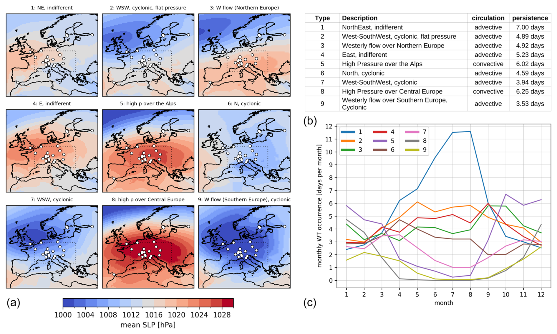
Figure 1 (a) Climatological average of sea level pressure in 1957–2020 for CAP9 WTs. White-filled circles indicate station locations (see Sect. 2.2). The dotted rectangle represents the wider Alpine area for which the CAP9 WT classification is representative. (b, c) Description of CAP9 WTs, including their average persistence [d] in the period of 1957–2020 (b) and their average monthly occurrence in 1957–2020 (c).

For our reconstruction, the WT classification must be assumed to be stationary over time, meaning that the dominant circulation patterns over central Europe remained the same for the last 300 years. Our WT reconstruction thus does not yield information on whether the characteristics of the prevailing synoptic situations changed, which, due to the scarcity of data for the earlier periods covered by our reconstruction, is not possible. This stationarity assumption is further discussed in Sect. 3.

2.2 Station observations

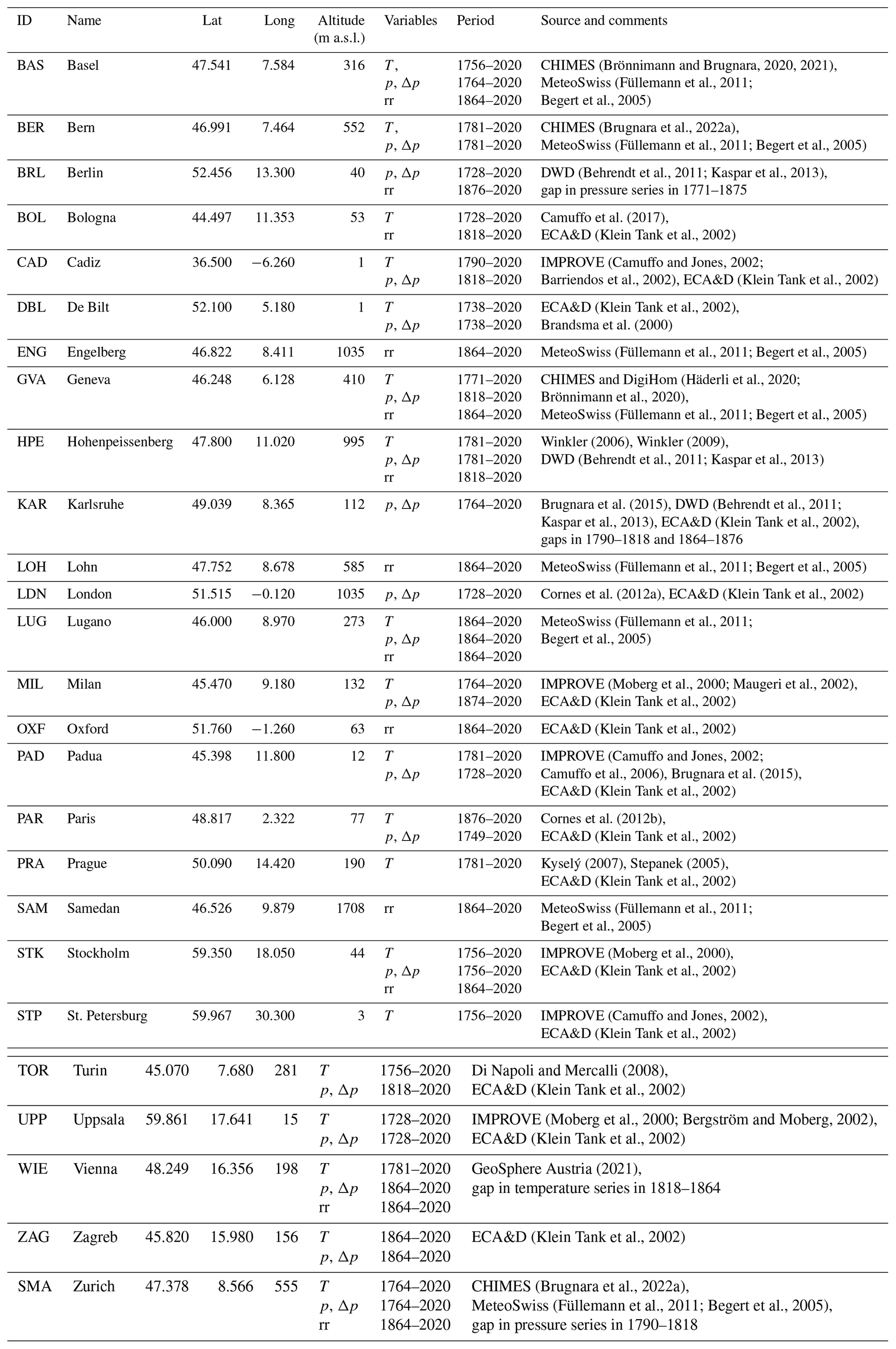
Meteorological observations used for WT reconstruction are located around and within the greater Alpine region in central Europe, for which the CAP9 classification is representative (Fig. 1; see also Weusthoff, 2011). Note that the available stations are relatively well distributed across central Europe, which is crucial to capture the large-scale synoptic situation. However, in southern and eastern Europe, unfortunately the available digitised station records were scarce. While the CAP9 classification is based solely on sea level pressure data, the station observations used for our reconstructions also include other variables, i.e. temperature and categorical rain data. Sea level pressure represents the synoptic atmospheric flow, whereas the other variables represent the associated surface effects and thus may provide valuable additional information for WT reconstruction (Schwander et al., 2017), especially in the context of the early-instrumental period with scarce data availability. A summary of the available daily station records is given in Table 1, with the data source indicated in the last column.

(Brönnimann and Brugnara, 2020, 2021)Füllemann et al., 2011Begert et al., 2005(Brugnara et al., 2022a)(Füllemann et al., 2011; Begert et al., 2005)(Behrendt et al., 2011; Kaspar et al., 2013)Camuffo et al. (2017)(Klein Tank et al., 2002)Camuffo and Jones, 2002Barriendos et al., 2002(Klein Tank et al., 2002)(Klein Tank et al., 2002)Brandsma et al. (2000)(Füllemann et al., 2011; Begert et al., 2005)Häderli et al., 2020Brönnimann et al., 2020(Füllemann et al., 2011; Begert et al., 2005)Winkler (2006)Winkler (2009)(Behrendt et al., 2011; Kaspar et al., 2013)Brugnara et al. (2015)Behrendt et al., 2011Kaspar et al., 2013(Klein Tank et al., 2002)(Füllemann et al., 2011; Begert et al., 2005)Cornes et al. (2012a)(Klein Tank et al., 2002)Füllemann et al., 2011Begert et al., 2005(Moberg et al., 2000; Maugeri et al., 2002)(Klein Tank et al., 2002)(Klein Tank et al., 2002)Camuffo and Jones, 2002Camuffo et al., 2006Brugnara et al. (2015)(Klein Tank et al., 2002)Cornes et al. (2012b)(Klein Tank et al., 2002)Kyselý (2007)Stepanek (2005)(Klein Tank et al., 2002)Füllemann et al., 2011Begert et al., 2005(Moberg et al., 2000)(Klein Tank et al., 2002)(Camuffo and Jones, 2002)(Klein Tank et al., 2002)(Moberg et al., 2000; Bergström and Moberg, 2002)(Klein Tank et al., 2002)GeoSphere Austria (2021)(Klein Tank et al., 2002)(Brugnara et al., 2022a)(Füllemann et al., 2011; Begert et al., 2005)

Table 1 Daily meteorological data used for WT reconstructions. T is temperature, p is pressure, Δp is the temporal pressure gradient, and rr are wet days.

For the comparison of reconstruction methods (Sect. 3.1), we use the same set of stations and variables that were used by Schwander et al. (2017) without any further preprocessing (see the SMD station sets in Fig. 2). This encompasses station records from London (Cornes et al., 2012a), Milan, Uppsala, Stockholm (Moberg et al., 2000; Maugeri et al., 2002), Turin (Di Napoli and Mercalli, 2008), Prague (Kyselý, 2007; Stepanek, 2005; Brázdil et al., 2012), Hohenpeissenberg (Winkler, 2009), De Bilt (Klein Tank et al., 2002), Paris (Cornes et al., 2012b, only temperature), Bern, and Lugano (Füllemann et al., 2011; Begert et al., 2005). Using the same data allows a direct comparison between our machine learning approaches and the Mahalanobis-distance-based method used in Schwander et al. (2017). In accordance with the latter study, daily mean temperature, sea level pressure, and the computed pressure difference vs. the previous day (Δp; see Table 1) were used as input variables for this comparison.

Further early-instrumental station series have been made available as a result of data rescue efforts in recent years (Brönnimann et al., 2019; Brugnara et al., 2020b), enhancing the data coverage in our area of interest and extending the period for which WTs can be reconstructed. Unfortunately, the majority of available records cover only a few years and thus are not suitable for our purposes. Using short observation records would lead to varying sets of stations, which, on the one hand, would introduce inconsistencies in reconstructed WTs and, on the other hand, constitute immense computational efforts, as for each set of stations, a new model has to be trained. Further issues arise from inhomogeneities in the observation series in time (e.g. observation errors, artificial trends or shifts), which originate from changes in instruments or observation sites, as well as various error sources related to early-instrumental data (see e.g. Brugnara et al., 2020a; Winkler, 2006; Böhm et al., 2010). Such inhomogeneities would again lead to errors or biases in the reconstructed WT series.

Where possible, long-term homogenised station records that contain no or only a few and short gaps were used for our approach. For some locations, however, multiple historical observation records from the same location had to be merged into a single time series. For the temperature series from Bern, Basel, Geneva, and Zurich, we benefitted from previous efforts to merge and homogenise daily temperature series (Brugnara et al., 2022a). Only stations at close locations, i.e. within a radius of less than 15 km, have been merged, with the exceptions of Cadiz (merged with T and p data from Huelva) and De Bilt (merged with T data from Haarlem and p data from Zwanenburg, Haarlem, Den Helder, and Delft), where the existing series could not be complemented with nearby station records. Complementary series have been retrieved from the ECA&D database (Klein Tank et al., 2002), as well as from the databases of MeteoSwiss (Füllemann et al., 2011; Begert et al., 2005); the German weather service DWD (Behrendt et al., 2011; Kaspar et al., 2013); the Royal Netherlands Meteorological Institute (KNMI; Brandsma et al., 2000); and GeoSphere Austria (2021), formerly the Austrian Central Institution for Meteorology and Geodynamics, ZAMG. The station sets used for the method comparison and the reconstruction of CAP9 WTs (Sect. 3.1 and 3.3) are summarised in Fig. 2 and labelled according to their respective start dates. While the comparisons in Sect. 3.1 use temporal pressure gradients as input, these gradients were omitted for the CAP9 reconstructions (Sect. 3.2 and 3.3), as tests (not shown) did not reveal consistent improvements by adding this variable.

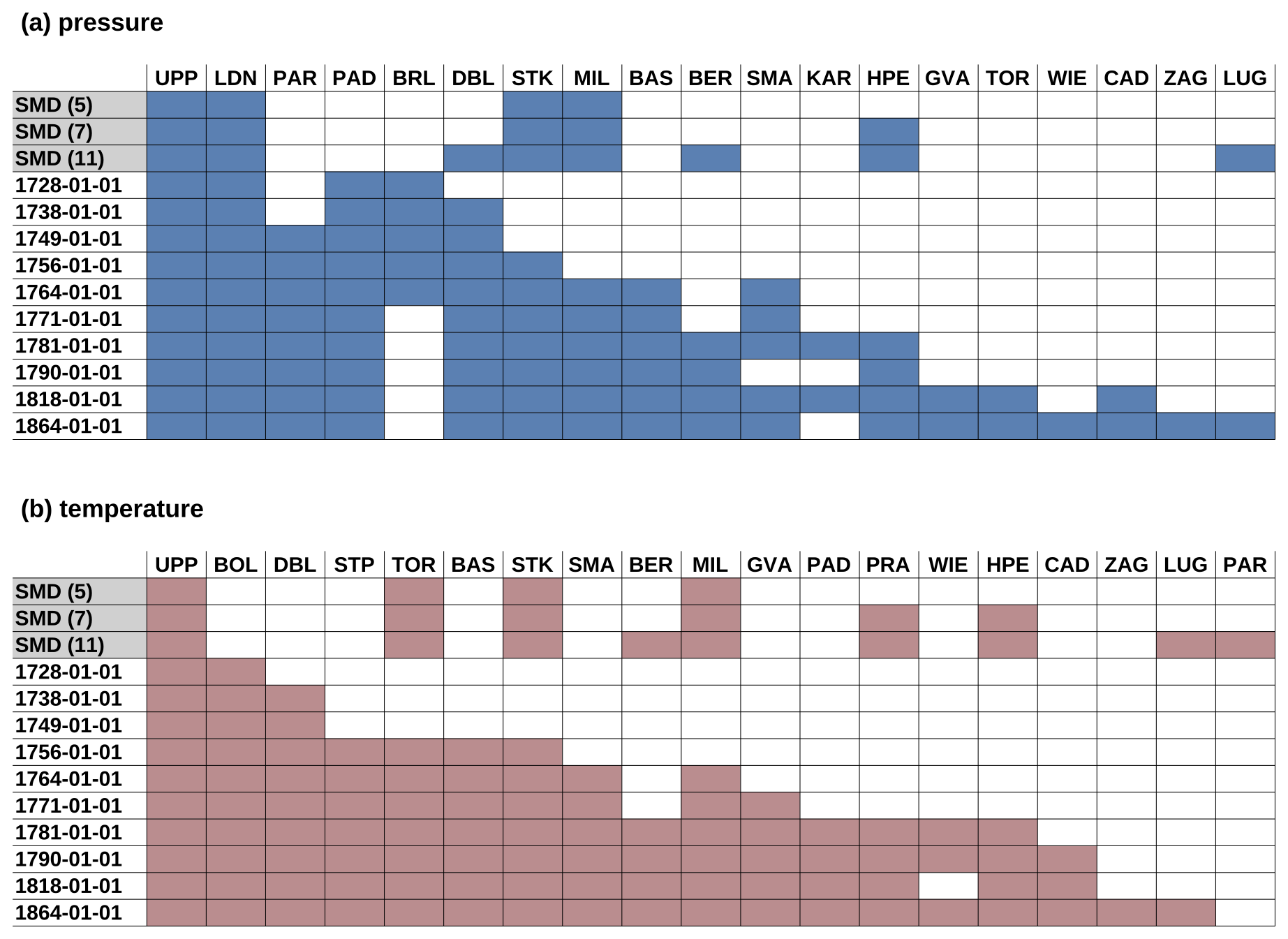
Figure 2 Station sets of (a) sea level pressure and (b) temperature used for the model comparison and WT reconstruction. The top three rows (SMD, grey shaded) refer to the station sets in Schwander et al. (2017) with 5, 7, and 11 stations, respectively. Station sets indicated by a date are used for the CAP9 reconstruction. The date refers to the start date of the respective station set. Data availability is indicated by the filled blue (pressure) and red (temperature) squares.

While in Schwander et al. (2017) observation records were not homogenised, we deemed it suitable to apply such a procedure to all pressure and temperature series that had not been homogenised, as well as to the merged series. We used the break point detection approach by Wang and Feng (2018), combining a penalised maximal t test (Wang et al., 2007) and a penalised maximal F test (Wang, 2008). As reference series, we used monthly pressure and temperature series extracted for the station locations from the EKF400v2 reanalysis (Valler et al., 2022). For further details on this homogenisation approach, see Imfeld et al. (2023). Most of the homogenised station records exhibit no or smaller gaps, with a median of 31 d. All gaps up to a length of 5 years were imputed with a k nearest neighbour approach, following Batista and Monard (2002). This is the same approach used by Schwander et al. (2017) for their WT reconstructions, thus maintaining consistency in our datasets. Tests for the imputation approach with 25 % randomly introduced gaps revealed an average bias of −0.063 hPa (−0.05 °C) and a mean absolute error of 1.83 hPa (1.46 °C) for pressure (and temperature). We thus deemed this method suitable for the task of WT reconstruction. The series from Berlin, Karlsruhe, Vienna (temperature), and Zurich (pressure) have longer gaps in their station records, which were kept.

Further preprocessing was necessary to use the station observations in the different machine learning models (the results of the respective assessments are not shown). First of all, a global warming trend is visible in all temperature records. In order to establish robust classification models, such non-stationarities in the data had to be removed. Temperature trends were removed individually for each series using a third-order polynomial fit. Furthermore, the pronounced seasonality of temperature might blur the temperature signals originating from atmospheric dynamics and lead to inhomogeneous treatment of weather types throughout the year. Thus, temperature data were corrected for seasonality by fitting the first two harmonics to each temperature record and then subtracting these harmonics from the data. Pressure and precipitation data have not been corrected for a trend or seasonality, which contribute only a negligible part to the total variability in these variables. All variables from all stations were standardised (i.e. by subtracting their average and dividing by their standard deviation). An important point to mention is that pressure gradients, and thus atmospheric patterns, are less pronounced in summer than in winter (see, e.g. Fig. 5 in Sect. 3.3). Although the general spatial distribution of the pattern remains similar throughout the year, the same WT shows different pressure amplitudes depending on the season. This might lead to seasonal inconsistencies in the WT reconstructions (see the discussion in Sect. 3.1 and 3.3). To correct for this issue, a monthly standardisation of pressure was tested (not shown). However, this degraded the reconstructions and was thus dismissed.

2.3 Machine learning approaches

For our model comparison (Sect. 3.1), multiple machine learning models are tested and compared against a baseline WT classification approach. This baseline model is given by the simple statistical classification approach from Schwander et al. (2017) for their CAP7 reconstructions and is based on the shortest Mahalanobis distance (SMD) of station observations to the centroids (station data averages) for each WT previously calculated from the reference period data. Further details on this approach are expounded in Schwander et al. (2017). The focus of this section lies on the ML approaches, including a multinomial logistic regression model, a random forest model, feedforward neural networks, and recurrent and convolutional neural networks. The best-performing model is then selected for the reconstruction of daily CAP9 WTs back to 1728 (see Sect. 3.3).

2.3.1 Multinomial logistic regression (MLG)

Multiple logistic regression is a commonly used method for classification problems with a categorical outcome. With a multiple-logistic-regression model, we can predict the occurrence probability p of a weather class WT as a function of several different station observations $x_{\mathrm{1}},x_{\mathrm{2}},\mathrm{\dots },x_n$ as independent variables (Hosmer and Lemeshow, 2000). While multiple logistic regression can predict only a binary dependent variable y, multinomial logistic regression can handle several response classes (if they have no natural order). The occurrence probability p(x) is defined as

$$y=p\left(x\right)={\displaystyle \frac{\mathrm{1}}{\mathrm{1}+e^{(-g(x\left)\right)}}},\text{where}\mathrm{0}\le p\left(x\right)\le \mathrm{1}.$$

The model is based on a linear regression function g(x):

$$g\left(x\right)={\mathit{\beta }}_{\mathrm{0}}+{\mathit{\beta }}_{\mathrm{1}}{x}_{\mathrm{1}}+{\mathit{\beta }}_{\mathrm{2}}{x}_{\mathrm{2}}+\mathrm{\dots }+{\mathit{\beta }}_n{x}_n.$$

The regression coefficients β_n are computed by applying the maximum likelihood method to maximise the probability, meaning that the coefficients are determined iteratively. For details, see the documentation of the R caret package (Kuhn, 2008).

Compared to complex and more advanced machine learning methods, logistic regression has the advantage of interpretability, as the relationships between the predictors and predictand can be directly inferred. One major drawback, however, is that often only a small number of covariates can be used in a model, as an increasing number of covariates may be subject to multicollinearity, which consequently can lead to overfitting of the model. To avoid this, we limited the number of predictors to five and constrained the variance inflation factor (VIF) to values below four. Model overfitting is further restrained by the training procedure (see Sect. 2.4). Furthermore, one has to keep in mind that logistic regression only allows for a linear combination of covariates; thus nonlinear features in the predictor data with respect to WTs are not captured by MLG.

2.3.2 Random forest (RF)

The second machine learning approach assessed in this paper is random forests (RFs) (Ho, 1995; Breiman, 2001). In contrast to single decision trees, RF use an ensemble of decision trees built from subsamples of the training data. With an increasing number of trees, the generalisation error in RF models decreases, and robust predictions can be established. In the case of our classification application, RF can provide a probabilistic estimate of the true WT using its ensemble of decision trees. Compared to other machine learning approaches, RFs are fast to train (depending on the number of trees) but can suffer from overfitting. In order to find a RF architecture with an optimal balance between accuracy and generalisability, several parameter sets are tested. These encompass the number of trees (between 10 and 400), the maximum depth (between 5 and 30), the minimum sample size for splitting (between 2 and 10), and the minimum sample size for a leaf (between one and four). Furthermore, the Gini impurity and entropy were tested to determine the splits. For further information, see the documentation of the scikit-learn Python package (Pedregosa et al., 2011).

2.3.3 Feedforward neural network (NN)

The third approach is feedforward neural networks (NNs) (Rosenblatt, 1958; Hastie et al., 2009). Similar to the RF approach, NNs provide estimates of probability for each class, represented by the normalised weights of the output layer. The NN architecture used for our work is not based on a predesigned NN model. While we prescribed the use of multiple layers, including a dropout layer before the output layer to avoid overfitting, optimal architectural properties such as the number of layers and their sizes were determined from scratch using a hyperparameter search on the training data (see also Sect. 2.4). In particular, networks with a number of layers between two and eight were tested with layer sizes between 32 and 256 (in steps of 32). Furthermore, dropout rates between 0.05 and 0.2 (in steps of 0.05), as well as learning rates between 10⁻⁴ and 10⁻², were tested during model tuning. The models were trained using the Adam optimisation algorithm (Kingma and Ba, 2014) and the categorical cross-entropy loss function. We set the batch size to 200 and the maximum number of epochs to 50 (with early stopping with a patience of 5 epochs). The NN approach, as well as the other neural network approaches, was implemented using the Tensorflow (Abadi et al., 2016a, b) and Keras (Chollet, 2021) libraries.

2.3.4 Recurrent and convolutional neural network (RNN and CNN)

Both the RF and the NN models described above use input data from the same day as predictors. As circulation patterns can persist for several days, it might be beneficial to also include information from preceding days in our models. For this reason, we assess both recurrent neural networks (RNNs) and one-dimensional (1D) convolutional neural networks (CNNs) in this study. For the RNN, we used long short-term memory networks (LSTMs) that can retain or discard information from previous time steps, and are thus able to propagate relevant information over multiple time steps (Hochreiter and Schmidhuber, 1997). Our RNN follows the same architecture as the NN, again with a dropout layer before the output layer and the same settings for model training. For reasons of computational costs, fewer architectural configurations were assessed than for the NN (i.e. between two and five layers with sizes between 32 and 128).

Similar to RNNs, convolutional neural networks (CNNs) can also make use of data from previous time steps. While a CNN is mostly applied to image data or to other multidimensional datasets for pattern detection using trained filters (Fukushima, 1980), we used its 1D equivalent for time series analysis (Kiranyaz et al., 2021). Similarly to the RNN, a reduced set of architectural properties (i.e. between two and five layers with sizes between 32 and 128) has been assessed, while the rest of the tunable parameters were kept identical to the other networks.

For both time-dependent neural networks (RNNs and CNNs), we used data from 2 d prior to the day of interest (3 d in total) to predict the WTs. A longer time window did not to yield improvements in the results (not shown). Analogous to NNs, RNNs and CNNs were also trained using the Adam optimisation algorithm with the categorical cross-entropy loss function, a batch size of 200, and a maximum of 50 epochs with early stopping.

2.4 Hyperparameter tuning and validation

Training and validation of the machine learning approaches were performed with the data described in Sect. 2.1 and 2.2, using the station observations as predictors and the CAP9 WT classification as the predictand. For the model comparison (Sect. 3.1), temperature, pressure, and temporal pressure gradients were used as predictors, as in the baseline approach (Schwander et al., 2017). The CAP9 reconstructions (Sect. 3.2 and 3.3) only use pressure and temperature series, as tests revealed no consistent improvements when including pressure gradients (not shown). After preliminary tests with certain subsets of stations and atmospheric variables (not shown), which did not yield any clear gains in performance, we chose to use the full set of stations and variables (pressure and temperature) available for the respective periods. For their approach, Schwander et al. (2017) used a reduced set of seven WTs (CAP7). Two pairs of WTs, 5 (high pressure over the Alps) and 8 (high pressure over central Europe), as well as 7 (west–southwest, cyclonic) and 9 (westerly flow over southern Europe, cyclonic) were combined into single WTs, as they were found to be too similar to distinguish. In order to compare our machine learning models to the SMD approach in Schwander et al. (2017) in the model comparison (Sect. 3.1), our models are trained on the same station data as was used in the original study but with the CAP9 WT series as the predictand. To make validation measures comparable to the baseline model, CAP9 classes are subsequently converted into CAP7 by combining the pairs of WTs accordingly. Also, the reference period for the model comparison (Sect. 3.1) was chosen similar to the baseline study by Schwander et al. (2017), spanning 1 January 1961–31 December 1998. For our new WT reconstructions (Sect. 3.3), we made use of the full available period for model training, spanning 1 September 1957–31 December 2020, and used the CAP9 classification for the evaluation.

Note that the same data are used for both hyperparameter tuning and validation of the models. In order to ensure independence between model tuning and evaluation, a nested cross-validation (Cawley and Talbot, 2010) is implemented. For the RF and neural network approaches, an outer loop splits the data into training and independent test sets. An inner loop is applied to the training set for hyperparameter tuning, again splitting off part of the data for validation of the model configurations in order to find the optimal hyperparameters independent from the training data. The outer loop then serves to independently estimate the validation metrics. Optimal hyperparameters are determined using Bayesian optimisation (Snoek et al., 2012). A total of eight folds for the outer loop and seven folds for the inner loop, without shuffling and without overlap, are applied. For the MLG model, we followed the same structure of outer and inner loops but with 10 outer and 10 inner folds (with overlap) instead of 8 and 7. The outer loop splits the data randomly into 80 % training and 20 % independent testing datasets. The inner loop uses the 80 % folds to find the best combination of station variables, again splitting the data into 70 % for training and 30 % for validation. We find the best combination and best number of predictors manually using a bidirectional stepwise approach, looking at mean performance, significance, and the z values of predictors. Once a model was found that worked well on all 10 inner folds and showed a good balance between over- and underfitting, we retrained it with the 80 % sets and evaluated it with the independent test sets (20 %) in the outer loop.

As Schwander et al. (2017) did not perform an independent validation of their approach, the validation measures are not comparable. For this reason, we reconstructed their approach and applied a cross-validation with the same training and test splits as in the eight outer loops described above. Results from this independent cross-validation can be directly compared to our approaches. When reconstructing the Mahalanobis distance approach of Schwander et al. (2017), an error in their model setup became apparent: when calculating the distance to each WT centroid using the covariance matrix derived for the respective WT, considerably lower accuracies than indicated in the original study were obtained (not shown). However, when using the covariance matrix from the true (observed) WTs, which of course would be unknown for the reconstructions, accuracies reached the values from the original study. For our validation of the SMD approach, the distance was calculated for each WT centroid using the correct covariance matrix of the respective WT.

Model performance is estimated using the overall accuracy and average Heidke skill score (HSS; Heidke, 1926; Cohen, 1960) values for all WTs and all seasons. The overall accuracy represents the fraction or percentage of days for which the WTs were correctly classified. The HSS represents the proportion of correct predictions scaled by the expected correct forecasts due to chance for categorical forecasts (see Hyvärinen, 2014) and is calculated for each WT. In contrast to overall accuracy, the HSS accounts for differences in the occurrence of individual WTs. To obtain a robust and independent estimate of the true performance of the best models, an average of these validation measures is taken over the outer folds of the nested cross-validation (i.e. 10 and 8 test sets for MLG and the other approaches, respectively). Note that the model used for the WT time series reconstruction is retrained with the full available dataset within the validation period. The accuracies indicated for the individual models are thus arguably pessimistic.

3 Results and discussion

3.1 Model intercomparison for CAP7 weather types

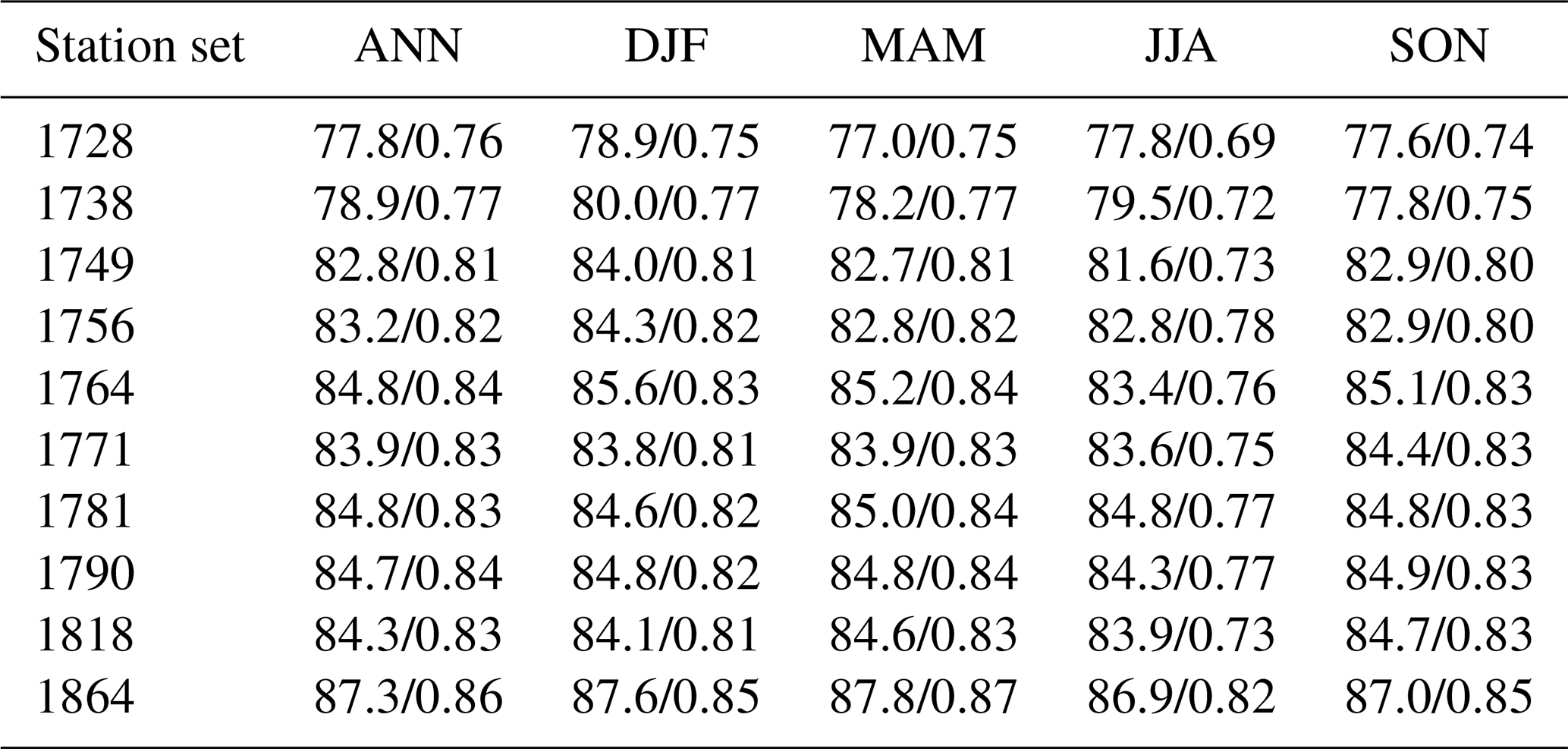
The performance of the WT classification approaches presented in Sect. 2.3, as well as the SMD approach by Schwander et al. (2017) for the CAP7 WT classification, is indicated in Table 2. The accuracies and HSS shown represent an average from the k-fold cross-validation over the period of 1 January 1961–31 December 1998 (see Sect. 2.4) based on three different subsets with data from 5, 7, and 11 stations, as was used in Schwander et al. (2017) (see also Table 3 therein). For the logistic regression model, only results from the optimal selection of station series is shown (see Sect. 2.3). The best-performing MLG model uses the following six variables: pressure in Milan and Paris, temperature in Prague and Stockholm, and the temporal pressure gradient in Milan and Stockholm.

Table 2 Validation metrics of all approaches applied for the CAP7 WT reconstruction, as well as the baseline model (SMD, in italics) using different data subsets. The value before the slash indicates the average accuracy in percent; the value after the slash indicates the Heidke skill score. Shown are values for the whole year (ANN) and for the individual seasons (winter – DJF; spring – MAM; summer – JJA; autumn – SON). The highest values per station set are marked in bold.

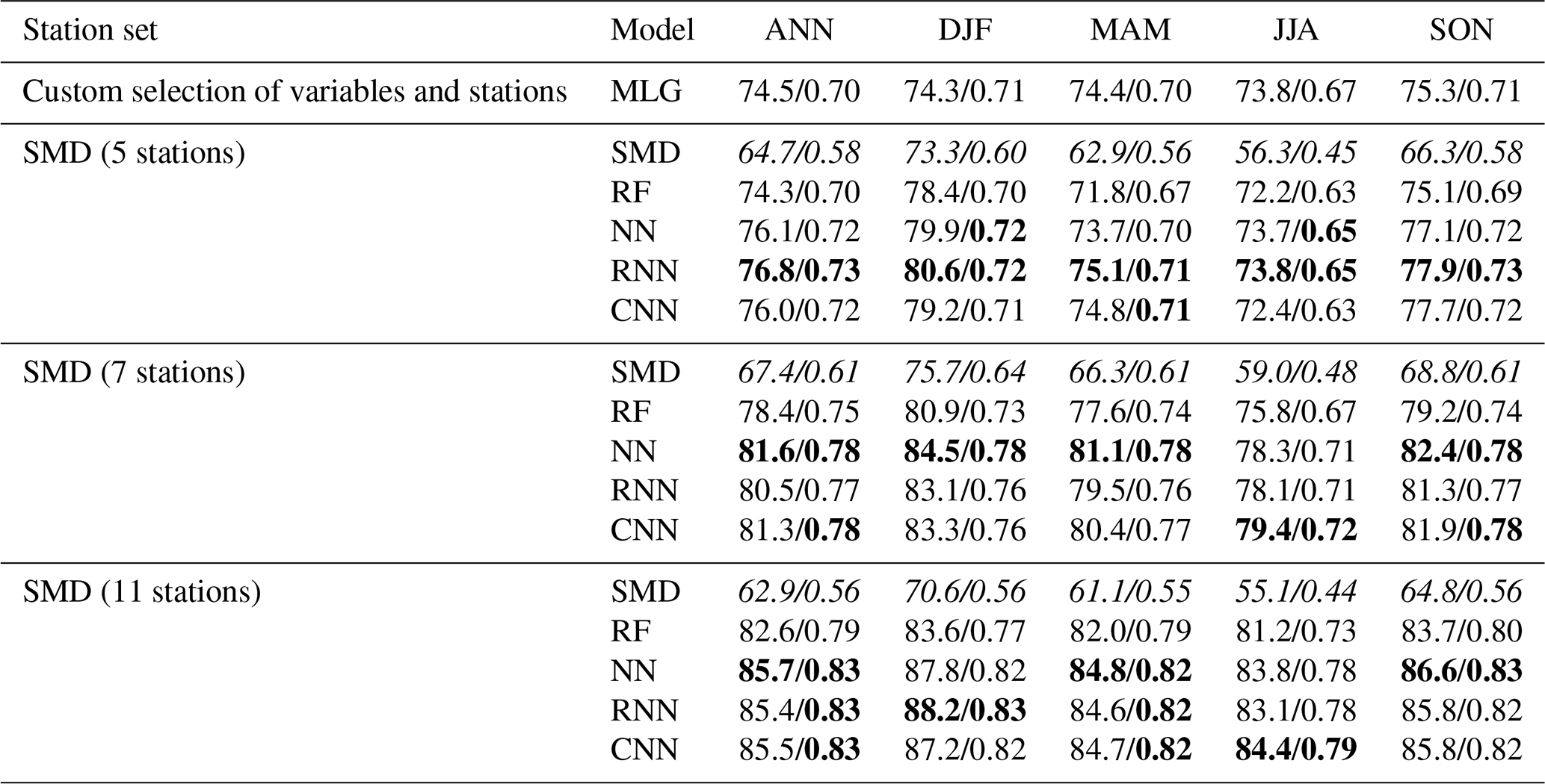
Evidently, all ML approaches outperform the baseline model (SMD, in italics) for all sets of stations. With an independent validation and correcting the error in the SMD model (see Sect. 2.4), accuracies are by far lower than indicated in Schwander et al. (2017), dropping below 70 % overall and below 60 % in the summer months. The machine learning approaches show accuracies of about 75 % even for the smallest set of stations (and the selection of the MLG). Accuracies of the RF models are typically lower by 2 %–3 % compared to the neural networks, regardless of the station set. Validation measures improve with the number of stations, reaching a maximum overall accuracy of 85.7 % for the NN model with 11 stations. Note that in contrast, the SMD approach shows lower accuracy values for the largest station set than for the other two, pointing to issues arising from data quality or the spatial distribution of the station network for this approach. The Heidke skill score (HSS) shows a similar pattern, with scores between 0.7 and 0.83 (compared to values between 0.56 to 0.61 for SMD). The superiority of the machine learning approaches might be explained by their ability to (in theory) better fit nonlinear relationships and interactions in the data compared to common statistical approaches (see also Sect. 2.3).

From the seasonal validation measures, we see a slight drop in accuracy (stronger for the HSS) for spring and summer, which was also found in Schwander et al. (2017), especially for summer. Weaker pressure gradients hamper a robust detection of WTs for these months. The difference between spring–summer and autumn–winter, however, is much smaller for the machine learning approaches compared to SMD. All of our models are thus more capable of coping with seasonal differences, although some seasonal patterns in the accuracy remain.

Random forests and multinomial logistic regression allow some inference about the stations and variables that prove to be crucial for WT classification. Regarding the spatial distribution of the stations, it is not a high density of stations within the area for which the CAP9 classification is representative (see Fig. 1) but instead an even distribution of stations around the borders of this area that leads to the most accurate predictions. This becomes evident for the optimal selection in the MLG approach, with all predictors being highly significant in the model (p ≤ 0.05). The MLG coefficients for each covariant and for each WT are listed in the Supplement (Sect. S2), together with further illustrations displaying the relationship of each predictor to the probability of each class response in the model. Also, RF results underpin the fact that a spatially well distributed station network is crucial for a robust WT classification. This is not surprising, as for WT classification, the models benefit not from the localised effects in the station observations but from the information on the atmospheric state over a larger region. In this context, more stations located in southern, eastern, and also western Europe (see Fig. 1) could improve the accuracy of the models. Looking at the feature importance (i.e. for each feature (predictor), the average reduction in the Gini impurity or entropy in the split classes over all trees) in RF, pressure data show the highest importance, followed by temperature (see Sect. S3). The temporal pressure gradient, on the other hand, showed lower importance values by 1 order of magnitude compared to the other variables. These results are robust also in the MLG model, where pressure showed the highest importance, followed by temperature and the pressure gradient. We want to note, however, that the MLG models still always preferred a combination of all three types of information instead of using just pressure data. This holds equally for the other approaches, where preliminary tests using only pressure data vs. using all variables confirmed the use of our multivariate input data (not shown).

The model comparison revealed that on average the feedforward neural network (NN) exhibits the highest accuracy and HSS estimates, although only slightly better than those of RNN and CNN. Note that for particular station sets or seasons, RNN and CNN show better metrics than the feedforward NN. An interesting result is that, opposite to our expectations, including the temporal evolution of the previous days (linked e.g. to preferential WT transitions) as input in RNN and CNN did not yield clear improvements. While this temporal information may yield benefits when only a small number of input series is available (see the RNN results in Table 2), measurements from a single day are generally sufficient to correctly detect WTs. The NN can be considered the best model for another reason: in contrast to RNN (and a bit less so for CNN), it is considerably faster to train, making it favourable also from the computational resources perspective. Regarding this aspect, it is important to mention that the simplest approaches we tested (MLG, RF) are much less costly in terms of computation hours than neural networks. Depending on the task and the related goal of accuracy, using these simpler methods is thus highly recommended. From this point on, we will only use the feedforward neural network model for further analyses and for the final reconstruction.

3.2 The effect of categorical weather data

As stated in the introduction, ML approaches have the advantage of being able to process continuous and categorical information simultaneously. In this section, we assess the effect of including time series of wet days based on rain information (see Sect. 2.2) as additional model input, as they have proven to be very valuable for statistical weather reconstructions (Imfeld et al., 2023). For this purpose, we trained an NN model for two different station sets used for our new reconstruction (Sect. 3.3), once without and once with the categorical rain series. Model building and validation has again been performed as described in Sect. 2.4. We used the station set available from 1728 (fewest predictors – four pressure and two temperature series; see Fig. 2) and the one available from 1864 (most predictors – 17 pressure and 18 temperature series; see Fig. 2) to analyse the impact of adding categorical data for different numbers of predictors. Both station sets were complemented with 13 series of wet days (Sect. 2.2). Note that these categorical rain records do not go as far back as 1728 but mostly only to 1864 (see Table 1). In order to better illustrate the effect of adding categorical data, we decided to use all available wet-day series for both experiments.

For the 1728 station set without wet-day series, the overall accuracy is estimated at 77.8 % (see also Table 3). By adding wet days, this increased by 0.5 %, to 78.3 %. While for the autumn and winter months, the accuracy increased by 1 %, it declined by 0.5 % for the summer months. For the 1864 station set, adding wet days to the predictors decreased total accuracy by 0.8 %, to 86.5 % (compared to 87.3 % without wet days). Also, all seasonal accuracies show a decrease between 0.4 % and 1.3 %. This shows that adding wet-day series to the model input leads to negligible changes in accuracy, which are mostly within the range of uncertainty in model training (i.e. smaller than the variance of accuracy and HSS in the outer folds of model training). With very few pressure and temperature records available (i.e. for the 1728 station set), wet days can provide supplementary information for WT classification. However, in our case, improvements were limited to autumn and winter, where precipitation is largely determined by large-scale circulation, whereas for summer, the results are slightly less accurate when including rain observations, which is arguably linked to precipitation being more frequently driven by local convection. If abundant pressure and temperature series are available (i.e. for the 1864 station set), using wet days as predictors yields no benefits. In this context, we decided to omit wet-day series for our final CAP9 reconstructions in Sect. 3.3.

Table 3 Validation results for the feedforward NN models with different station sets (named after their starting year). The value before the slash indicates the average accuracy in percent; the value after the slash indicates the Heidke skill score. Shown are estimates over the whole year (ANN) and for the individual seasons (winter – DJF; spring – MAM; summer – JJA; autumn – SON).

3.3 Reconstructing CAP9 weather types, 1728–2020

3.3.1 Model performance and reconstruction quality

With the feedforward neural network (NN) outperforming the other approaches (Sect. 3.1), we extended the current WT series for the CAP9 classification back to 1728. In order to provide an estimate for the model performance and by that of the reliability of our CAP9 reconstructions, a validation procedure as described in Sect. 2.4 was applied. The station series (sea level pressure and temperature records) that have been used as predictors are described in Sect. 2.2. A summary of the resulting model architectures can be found in the Supplement (Sect. S4). Table 3 gives an overview of the validation results in the form of overall accuracy and average HSS for predicted CAP9 WTs vs. the original predictand time series (1957–2020) by MeteoSwiss for all station sets. The results are again given for the whole period and are distinguished by season. The accuracy achieved when using the smallest station set (stations available from 1 January 1728 to 31 December 1737) is already remarkably high, with a value of 77.8 % despite the limited set of available stations. Adding more station series generally improves the accuracy and skill score values (with some remaining variability depending on model training runs). Note that the validation metrics shown in Table 3 only provide values with respect to the reference period of 1957–2020. The actual values for the past periods may be lower due to larger uncertainties and errors in the data, but unfortunately they cannot be determined due to the lack of a historical reference WT series. While reconstructions for most station sets show slightly less skill and lower accuracies for the summer months (JJA), differences vs. the overall average remain small, with values of approximately 1 % for accuracy and 0.1 for the HSS. Those seasonal differences in model skill are arguably linked to the model being trained over the full year (see the discussion in Sect. 3.3.2).

To provide more insight into the patterns of correctly and wrongly classified WTs and the reasons why the model is not able to assign certain WTs correctly, further analyses have been performed. Figure 3 shows the confusion matrices for the station sets 1728 and 1864 for the reference period of 1957–2020. While accuracy may vary among the models, training runs, and station sets, the actual WTs that are wrongly assigned to each true class are similar. For the “extreme” WTs, 8 and 9, most false predictions – as expected – identified WTs 5 and 7, which show the most similar patterns to the correct WTs, 8 and 9, respectively (see Fig. 1). While Schwander et al. (2017) found these two WT pairs hard to distinguish and reduced the number of WTs accordingly, the NN model accuracies for WTs 8 and 9 are comparable to the other WTs. The NN model is thus capable of correctly distinguishing between these extreme (i.e. with respect to the intensity and extent of high- and low-pressure systems) WTs and their less extreme counterparts.

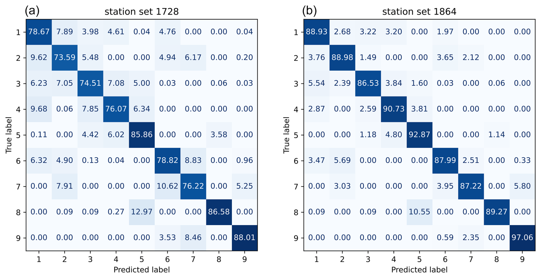
Figure 3 Confusion matrices for reconstructions (columns) with station sets 1728 (a) and 1864 (b) against reference CAP9 series (rows) for the reference period. Values are given as a percentage of the respective WT occurrence.

Figure 4 shows the patterns of pressure deviations from the average of the time series (in standard deviations) for each station and weather type within the reference period. Indicated are the average values for correctly assigned (blue) and wrongly assigned (red) WTs, as well as the range between the 5 % and 95 % quantiles (shaded areas) from the reconstruction with the 1864 station set. Deviations of the red and blue circles at individual/all observation points indicate regional/overall discrepancies in the observed pressure distribution as the reason for false detections. Coinciding red and blue circles mean that observation patterns of true and false predictions are identical and that the reason for the false predictions cannot be explained by the observations. Evidently, some WTs have very similar patterns with a large overlap (e.g. WT 5 and WT 8), making distinction difficult. For most WTs dominated by extremely high or low pressure (e.g. WTs 5, 8, and 9), wrongly assigned WTs are linked to more moderate values in the pressure data. Furthermore, regional differences in the pressure distribution can be identified as a source of error. For example, WT 6 is more likely to be confused with other WTs for days with stronger low-pressure systems over northern central Europe. Such regional patterns can also be found for WTs 3, 4, and 7. The corresponding temperature profiles (see Fig. S8) show similar patterns to observed temperatures for days with wrongly assigned WTs closer to the mean (WTs 2, 3, and 6) or regional differences (WTs 7, 8, and 9), although these patterns are much less distinct. The same evaluation for the other station sets provides similar results (not shown).

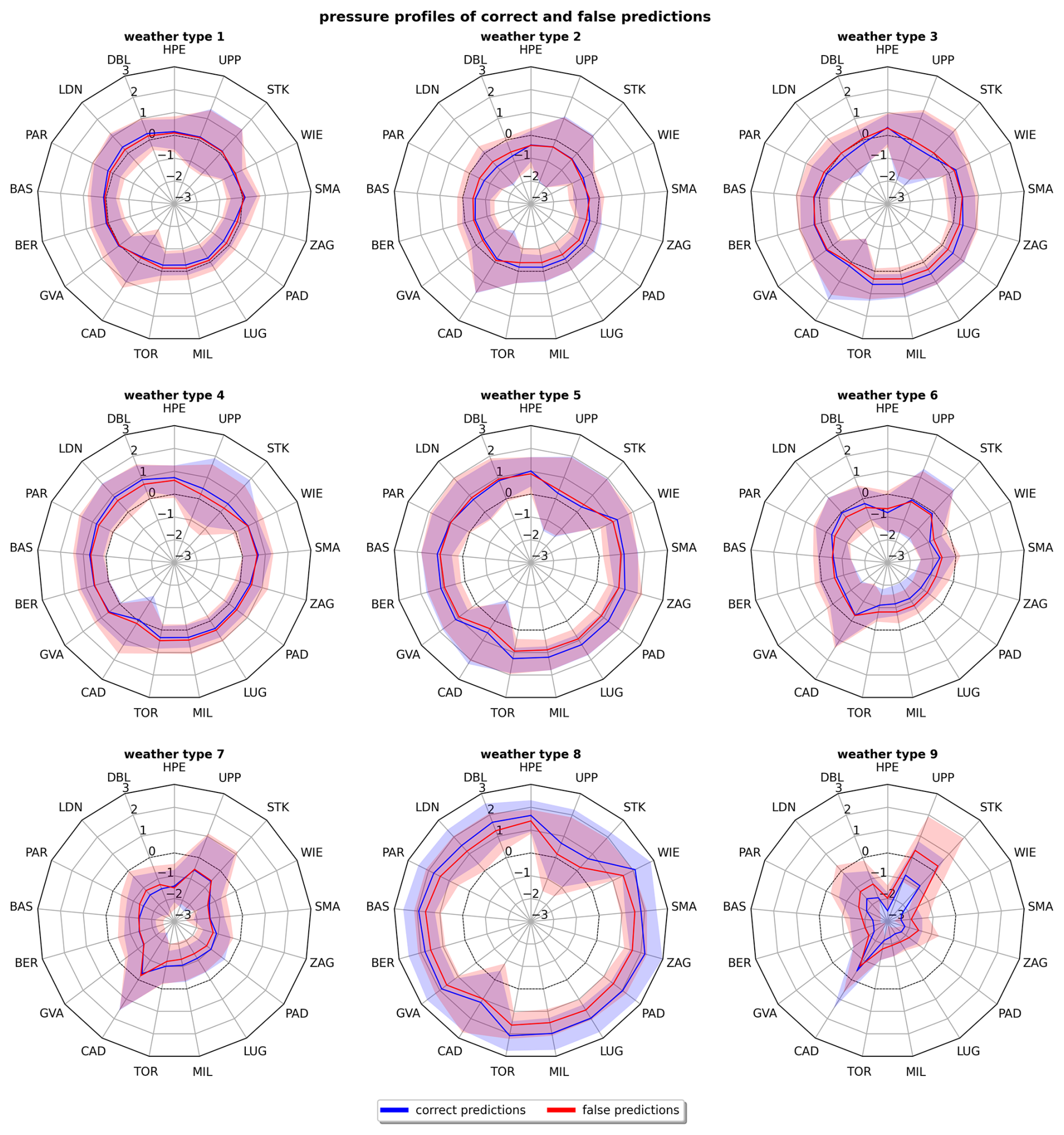
Figure 4 Station data pressure patterns for correct (blue) and false (red) predictions from the 1864 station set for all nine WTs. Shown are the average (lines) and the 5 %–95 % quantile interval (shaded areas) in units of standard deviations.

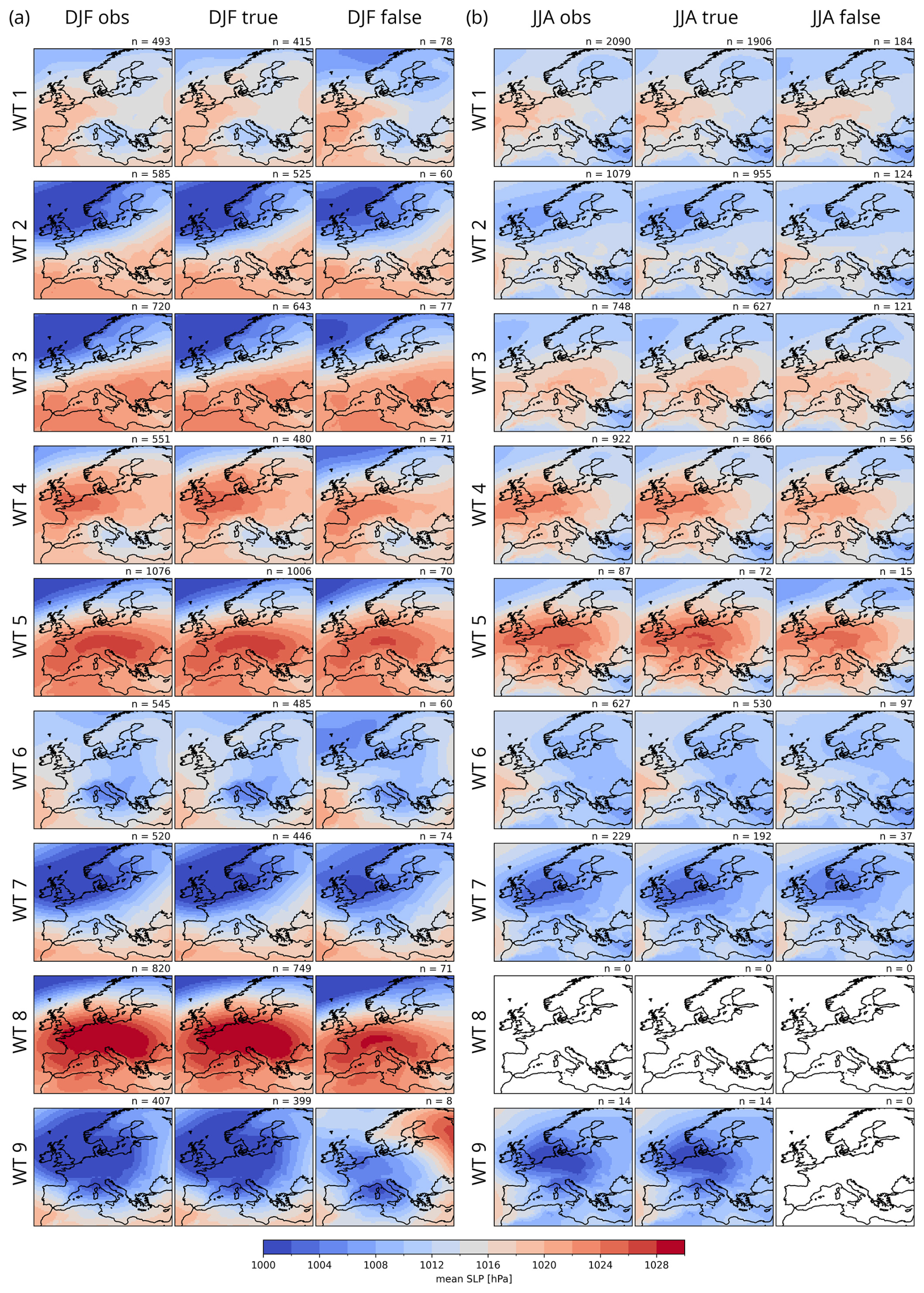
Figure 5 Climatological average of sea level pressure in 1957–2020 for CAP9 WTs for the (a) winter and (b) summer months. Shown in each panel are the averages according to the official WT series by MeteoSwiss (left, obs column), correctly predicted WTs (centre, true column), and wrongly predicted WTs (right, false column). The number of cases (n) is indicated in the top-right corner of each subpanel.

Figure 5 shows average sea level pressure maps for the period of 1957–2020 derived from ERA5 (Hersbach et al., 2020; Bell et al., 2021). The maps are separated by season, namely winter (DJF, Fig. 5a) and summer (JJA, Fig. 5b), as well as by reference series (top), correctly attributed WTs (centre), and false predictions (bottom). Note that WT 8 does not occur during the summer months (see the seasonality in Fig. 1, as well as Fig. S9) and that no day was wrongly assigned to WT 9 in the reference period, hence the empty panels in Fig. 5b. While false predictions for the winter months are strongly dominated by weaker-than-average pressure distribution rather than regional shifts, results are less clear for the summer months. While slight regional shifts are apparent (e.g. for WTs 1, 3, and 7), the reason for false predictions in summer seems to originate from other sources, arguably patterns in temperature or general difficulties of the model in capturing the smaller pressure gradients in this season.

Transitions between weather types may follow preferential patterns. A comparison of preferential transitions in the CAP9 reference series and reconstructions for the reference period from different station sets (Fig. S10a–c) did not show strong differences, although reconstructions show a small bias towards persistence. Our analyses furthermore revealed that those preferential transitions show only small changes throughout the reconstruction period (Fig. S10d–f). Preferential transitions between WTs are thus generally well represented in the CAP9 reconstructions. As the synoptic circulation is constantly changing, weather types might change over the course of 1 d. This has to be taken into account when analysing daily WT reconstructions, as such WT transitions may be a source of error. In the reference CAP9 series, 19.1 % of days are persistent weather situations, with the same WT on the days before and after. A majority of the days (46.4 %) have a partly transient situation, with the same WT on one of the neighbouring days and a different one on the other, and in 34.5 % of the cases, different WTs occur on both neighbouring days (transient situation). Taking reconstructions using station set 1864 as an example, the correctly classified WTs show the same percentages. For the days with false predictions, however, transient situations are overrepresented (48.0 %), whereas only 7.6 % show persistent conditions. We can conclude that transient situations play an important role as a source of uncertainty in daily WT reconstructions. The WT chosen for these cases is typically the one with the strongest imprint on the daily average station observations and not necessarily the one persisting throughout most of the day. Furthermore, a dominant WT might be chosen by a very small margin. This issue might be solved by introducing a neutral (transient) class or by calculating WTs for a specific time of the day (e.g. 12:00 UTC) using subdaily data that is, however, less readily available for the early-instrumental period.

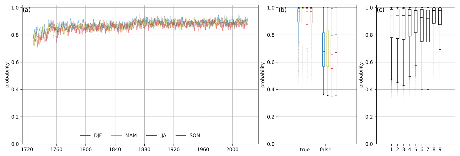
Figure 6 (a) The 1-year running mean of the daily maximum probability (fraction) of the reconstructed CAP9 WT series, separated by season. (b) Boxplots of the probability for correctly (true) and wrongly (false) attributed WTs within the reference period, separated by season. Panel (c) is the same as panel (b) but separated by weather type. The thick line indicates the median; the boxes extend to the quartiles and whiskers to 1.5 times the interquartile range.

The next interesting feature to look at is the confidence of the model in its predictions, i.e. the probabilities with which the WTs are classified. As stated in Sect. 2.3, for each day, the NN attributes a probability to all WT classes, and the class with the highest probability is selected as the predicted (or most likely) WT. Figure 6a (for comparison with the baseline approach, see Fig. S11) shows a 1-year running mean of the daily probabilities of the predicted WTs by season for the whole period of reconstruction. It shows values around 0.8 in the first 2 decades, increasing to values between 0.825 and 0.875 in the middle of the 18th century and to values between 0.85 and 0.9 in 1864. The fact that detection probabilities remain nearly constant at a high level over the last 300 years suggests that the stationarity assumption of the WT classification (see Sect. 2.1) is reasonable, as otherwise, larger shifts towards lower detection probabilities would be expected. Also the seasonal differences in detection probabilities are small. The distinction of daily maximum probabilities according to correct and false classifications in the reference period (Fig. 6b) reveals that the model used for our CAP9 reconstruction is less confident for WTs that were wrongly assigned (median = 67.4 %) than for correct attributions (median = 97.3 %). This is in line with the above finding on transient WTs, where mixed signals in the surface observations may lead to false classifications. Seasonal differences are again small, with only slightly lower values in summer, showing that the model being trained over the full year can be considered reasonable. The same applies to differences in detection probability between individual WTs (Fig. 6c). Only the two extreme WTs, 8 and 9 show slightly different patterns (i.e. higher probabilities).

3.3.2 The new CAP9 reconstructions in a climatological context

In this section, we look at the CAP9 WT reconstructions produced with the NN approach (Sect. 2.3) for the full period of 1728–2022. The aim is to analyse their quality and consistency, i.e. look for possible discontinuities in WT frequencies, as have, for example, been found for the Hess and Brezowski WT classification in the mid-1980s (Mittermeier et al., 2022). Furthermore, we compare occurrence frequencies of reconstructed CAP9 WTs with the CAP9 reference series on climatological timescales to analyse the representation of internal climate variability in WTs in the past decades to centuries. For a comparison with the WT reconstruction by Schwander et al. (2017), the supplement provides the figures presented in this section with the addition of the CAP7 reconstructions (see Figs. S11–S13).

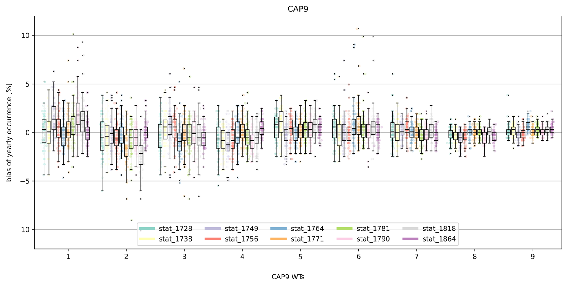
Figure 7 Bias of yearly WT occurrence (in % of days of the year) for all WTs (x axis) and station sets (colours) in the NN reconstruction.

An important quality characteristic is biases in the occurrence of different WTs. Figure 7 illustrates the percent bias (with respect to the number of days of the year) in yearly WT occurrence for the reference period (n = 63 years), separated by station set and weather type (for comparison with the baseline approach, see Fig. S12). The median biases remain within 1 %–2 % for all WTs and station sets, with no systematic over- or underestimation of an individual WT. Some outlier years are evident for WTs 1, 3, and 6 (overestimation), as well as WTs 2 and 3 (underestimation).

Figure 8 illustrates the full reconstructed time series of the yearly occurrence for each WT (in black), again with the CAP9 reference series (in red) for comparison (a comparison with the baseline approach is given in Fig. S13). For better readability, a 10-year running average is indicated. The yearly WT occurrence in our new CAP9 reconstruction shows high correlation values (average = 0.948) and relatively low root-mean-squared error values (average = 3.35 d). A positive bias for WTs 6 and 9, as well as a negative bias for WT 8 determined in Fig. 7, can also be seen in the time series. In the time series presented in Fig. 8, no apparent artificial discontinuities that go beyond natural variability can be determined, which is expected, as homogenised input data are used. In order to study discontinuities and trends in further detail, statistical tests were applied. To detect discontinuities (i.e. changes in the data structure) in yearly WT occurrence, we applied a pruned exact linear time (PELT) algorithm following Killick et al. (2012) (see also Truong et al., 2020), with the constraint that change points are 10 samples apart at least. Between 9 and 17 change points were detected over the full reconstruction period (Fig. S14). This analysis does not allow us to infer whether the discontinuities detected are artificial or whether they originate from natural variability. However, only a few common breakpoints between individual WTs are found, and the majority of detected discontinuities do not coincide with changed station sets in the input. This points to the fact that the discontinuities discovered are not introduced artificially and that our CAP9 reconstructions can be considered homogeneous over time. Long-term trends were examined using a Mann–Kendall test (Kendall, 1975) at a significance level of α = 0.05. No significant trends in the yearly occurrence have been found (see Fig. S15). These analyses support the stationarity assumption (see Sect. 2.1). If this assumption were not to pertain, a pronounced decline in the frequency of occurrence would be expected, as the predefined modern WTs would only rarely be observed in the distant past. For the yearly average persistence, however, statistically significant trends were determined for WTs 4 (decrease), 7 (decrease), and 9 (increase), although they were small in magnitude (see Fig. S16).

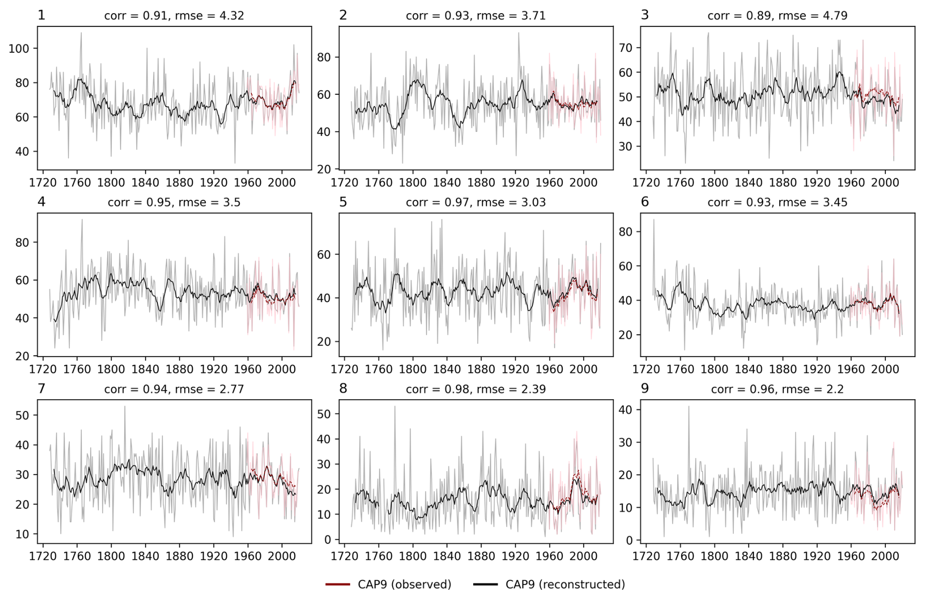
Figure 8 Yearly occurrence of reconstructed CAP9 WTs (lighter colours) with the 10-year running mean (darker colours). Shown are the CAP9 reference series (red) and the CAP9 reconstructions (black). The correlation and root-mean-squared error for the yearly WT occurrence with respect to the reference series are written above each subpanel.

More detail on the occurrence frequency is given in Fig. 9, where we show the 10-year running average yearly WT occurrence distinguished by season. These seasonal occurrence patterns of CAP9 reconstructions generally match the occurrence in the reference series. For WTs 6 and 9, the positive bias observed in the reconstructions can be mainly attributed to an overestimation of WT occurrence in spring (MAM). The negative bias of WT 8, on the other hand, is linked to an underestimation of this WT in the winter months (DJF). The attribution of a bias to seasonal differences points to an important issue in WT reconstruction. As most WTs (1, 5, 7, 8, and 9) show a pronounced seasonality, they can be difficult for a model that is trained over all seasons to predict. Tests training individual models for each season improved the results, although for some WTs (e.g. WT 8 in summer), the available sample for model training becomes too small. Another option might be to include seasons or months as categorical predictor variables, although this has not been tested in this study. Seasonal shifts in WT occurrence are assessed in Fig. S17. WT 1 exhibits a stronger seasonality in recent decades, whereas the seasonal variation in WTs 4 and 7 tends to decrease. The winter occurrence peak in WT 3 is shifted towards autumn, and WT 2 shows a tendency towards a second occurrence peak in summer. However, those seasonal shifts are small compared to the large year-to-year variability in WTs.

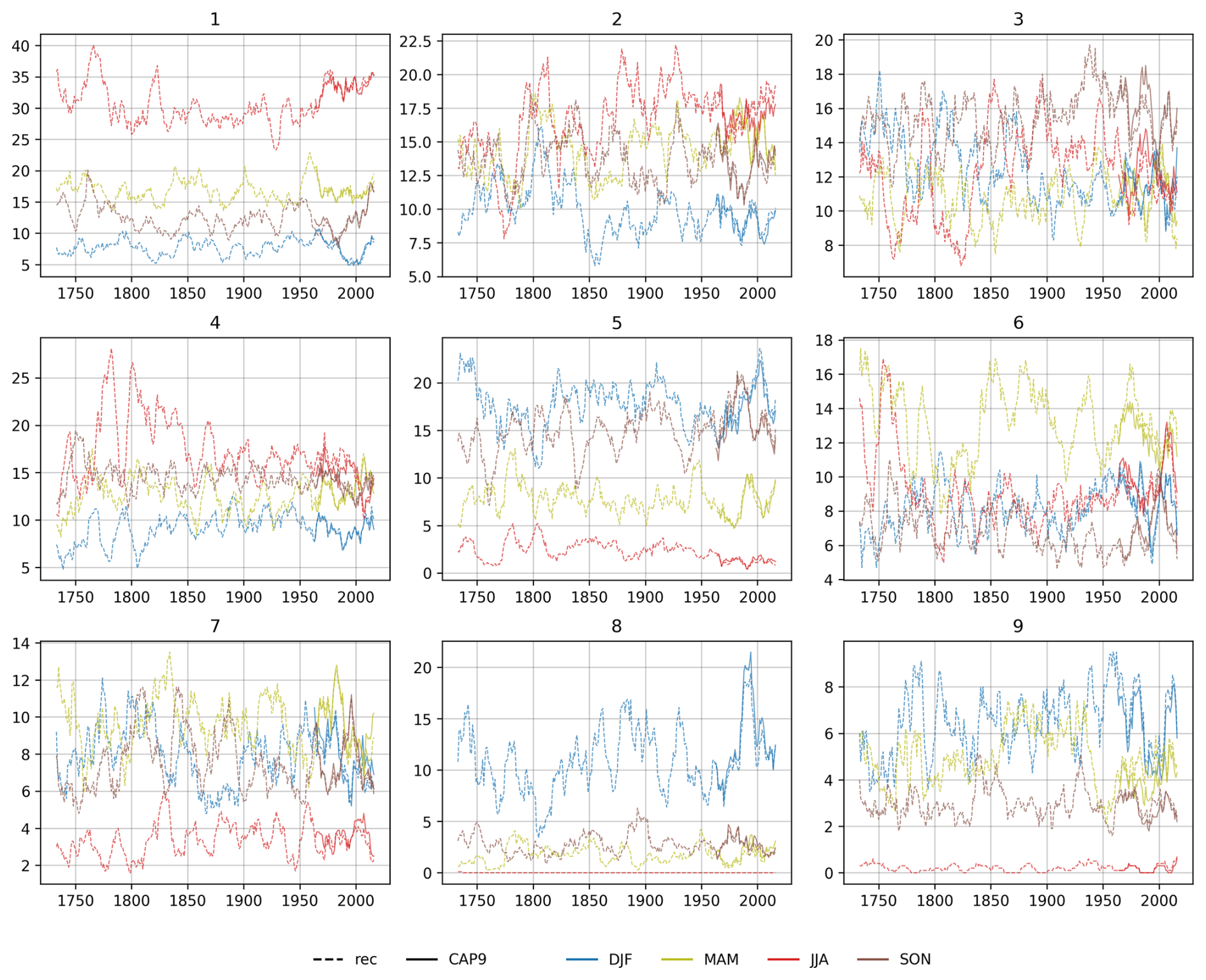
Figure 9 The 10-year running average of yearly WT occurrence by season (DJF – blue; MAM – green; JJA – red; SON – brown) and WT (the labels above each subplot). Shown are the CAP9 reference series (solid lines) and the CAP9 reconstructions (dashed lines).

4 Conclusions

In our study, we applied various supervised machine learning (ML) methods for station-based weather type (WT) reconstruction in order to assess their performance and to find an optimal ML approach for this purpose. With the model showing the best performance and using additional station observations, existing CAP9 WT series have been extended back to 1728.

Our results show that all ML approaches perform well when tested on the daily CAP7 WT classification. Independent estimates of accuracy and HSS show better performance of all models tested compared to the common statistical classification approach used as a baseline. ML methods can indeed profit from their ability to detect nonlinear patterns. The best-performing method varies between the three neural network approaches tested depending on the season, data used, and validation metric, although even the simpler and less computationally demanding multinomial linear regression and random forest approaches yield good results. Overall, the feedforward neural network was found to be slightly better than the other ML approaches and was therefore used to create the CAP9 WT reconstruction. The use of qualitative rain observations did not improve our reconstructions but instead yielded partially worse results and was thus omitted for our reconstructions. The extension of the existing CAP9 classification back to 1728 constitutes a novelty in WT reconstruction. The resulting WT time series proves to be accurate in various ways. No artificial trends or discontinuities were detected. The year-to-year variability and the seasonality of the WTs are well reproduced. Nevertheless, depending on the set of stations available, some over- and underestimation of WT occurrence was determined. Our results emphasise the importance of continuously improving methods of WT reconstruction when new options and data become available.

Some challenges or limitations related to our approach persist. First, the station data availability is usually scarce in the early-instrumental period. Further data rescue efforts may provide additional observations at important locations for WT classifications. Although our experiment with adding qualitative rain information did not improve the reconstructions, other qualitative information more directly linked to large-scale circulation, such as wind direction, might lead to improvements. Unfortunately, digitised, long-term wind direction records are sparse and therefore could not be assessed in this study. A second challenge is the occurrence frequency of each WT in the reference series. WTs with low occurrence frequencies and strong seasonality can pose a challenge for our WT reconstruction approach. Adding seasons as additional predictors or training different models per season could solve this issue, although the sample size of rare WTs might be too small. Also in general, the size of the training dataset has to be proportional to the number of WT classes in order to find robust model weights and biases. A third issue is the daily resolution of input and WT data: transient situations leave a mixed signal in the daily average observations, making the distinction at a daily resolution difficult. This issue might be solved with the use of subdaily data that are, however, less readily available in the form of long and homogeneous time series.

Our CAP9 reconstruction represents the longest daily WT series available and allows us to study decadal circulation variability in the context of past climatic changes, as well as the impacts of associated synoptic situations on the surface, e.g. extreme events. On the methodological side, future research may focus on including wind direction observations to improve and extend WT reconstructions even further back in time, although this requires tremendous digitisation efforts. While we focused on reconstructing CAP9 WTs, our ML models may be adapted to other WT classifications and regions.