Minimal influence of future Arctic sea ice loss on North Atlantic jet stream morphology

The response of the North Atlantic jet stream to Arctic sea ice loss has been a topic of substantial scientific debate. Some studies link declining Arctic sea ice to a weaker, wavier jet stream, which potentially increases the occurrence of extreme weather events. Other studies suggest no causal link between Arctic sea ice loss and the jet stream, instead attributing jet variations to internal variability. Current methods for characterising the low-level jet typically use zonal wind speeds averaged over the North Atlantic sector, which can result in the loss of important aspects of jet morphology. This study uses a new two-dimensional feature-based method to investigate the winter low-level jet response to future Arctic sea ice loss using idealised prescribed sea ice experiments from the Polar Amplification Model Intercomparison Project (PAMIP). In contrast to earlier studies that have focused on seasonal-average changes, this study also explores how daily jet variability is altered by sea ice loss. The results show a significant equatorward shift in mean jet latitude for three of the six PAMIP models analysed and a multi-model-mean equatorward jet shift of 0.6 ± 0.1°. Four of the six models show a significant weakening of the westerlies on the poleward side of the North Atlantic jet and a strengthening on the equatorward side. However, there is no change in jet speed and jet tilt across all models and no robust change in jet mass (area-weighted speed) when using the feature-based jet identification. Three of the six models show an increase in the frequency of split-jet days, but this does not strongly affect the overall distributions of daily jet latitude, speed and mass. Likewise, the results show no significant change in the daily variability in jet features, and changes in interannual variability are inconsistent between the models. The results extend previous studies characterising jet response from a zonally averaged perspective and suggest that it is unlikely that future Arctic sea ice loss will cause significant weakening of the North Atlantic jet stream or an increase in jet variability.

1 Introduction

In recent decades the Arctic has warmed at an accelerated rate compared to the global average, in a process known as Arctic amplification (England et al., 2021; Rantanen et al., 2022; Serreze et al., 2009; Serreze and Francis, 2006). As the Arctic has warmed, there has also been a rise in the frequency of extreme weather events in northern mid-latitudes, causing substantial interest in the possible role of Arctic warming in driving mid-latitude extremes (Barnes and Screen, 2015; Cohen et al., 2014, 2020; Francis and Vavrus, 2012; Shepherd, 2016).

The eddy-driven jet stream plays a key role in regional weather and climate in the mid-latitudes and can be affected by increases in greenhouse gases through several thermodynamic and dynamic mechanisms (Shaw, 2019). One possible mechanism linking Arctic amplification and extreme weather is through impacts on the mid-latitude eddy-driven jet stream. Sea ice loss is a driver of Arctic amplification, which weakens the meridional temperature gradient in the lower troposphere, potentially weakening the jet stream and causing an equatorward jet shift (Barnes and Screen, 2015; Cohen et al., 2020; Petoukhov and Semenov, 2010; Liu et al., 2012; Francis and Vavrus, 2012, 2015). This weakening may lead to increased wave amplitude or “jet waviness”, slower Rossby wave phase speeds, and more persistent weather patterns (Screen and Simmonds, 2014). Through these mechanisms, several studies have linked Arctic sea ice loss and recent mid-latitude weather to, for example, regional cooling trends over north-eastern America and eastern Eurasia (Inoue et al., 2012; Kug et al., 2015; Mori et al., 2019; Outten and Esau, 2012; Tang et al., 2013).

Other studies question the link between Arctic sea ice loss and extreme cold temperatures, with some model studies showing little or no changes in extremes with sea ice loss and instead attributing observed events to internal climate variability (Blackport et al., 2019; Cohen et al., 2020; Koenigk et al., 2019; McCusker et al., 2016). Smith et al. (2022) show a robust winter-average weakening and equatorward zonal-mean jet shift due to imposed Arctic sea ice loss in a multi-model ensemble. However, the amplitude of the signal was small compared to interannual variability, indicating only a weak atmospheric response to sea ice loss. The argument of Arctic warming driving a wavier jet stream has also been disputed, with some studies showing no decrease in wave speeds or an increase in wave extents (Barnes, 2013; Hassanzadeh et al., 2014; Blackport and Screen, 2020). Moreover, while the observational record spanning 1979 to 2012 suggests a correlation between Arctic sea ice loss and winter Eurasian cooling trends, extending the record to the present day reveals a diminishing relationship (Blackport and Screen, 2021; Smith et al., 2022). Therefore, the extent to which Arctic sea ice loss influences the jet stream and regional mid-latitude climate is not fully understood (Box 10.1. in Doblas-Reyes and Sörensson, 2021).

This study focuses on the lower-tropospheric component of the North Atlantic jet stream. A widely adopted framework for characterising the low-level jet is the jet latitude index (JLI; Woollings et al., 2010). The JLI has been applied to simulations from the Polar Amplification Model Intercomparison Project (PAMIP; Smith et al., 2019), which shows a small equatorward jet shift in the winter mean but no robust change in jet speed across models (Ye et al., 2023). However, Ye et al. (2023) focused on seasonal-mean changes and neglected short-term jet variability, which is often associated with extreme weather events. Ye et al. (2024) examined daily jet variability using the JLI and found an equatorward shift in the jet and weakening westerly winds with Arctic sea ice loss; however, they only used one climate model, so it is unclear if those findings reflect a wider range of models. Furthermore, the JLI used by Ye et al. (2024) adopts a one-dimensional view of the jet structure (Woollings et al., 2010) which neglects important jet characteristics related to tilted, split, weak and broad jets (Perez et al., 2024). Here, we use a new feature-based jet identification method (Perez et al., 2024) applied to PAMIP experiments to explore the effect of future Arctic sea ice loss on North Atlantic jet structure and its variability.

The remainder of the paper is laid out as follows: Sect. 2 describes the datasets and methodology used for characterising the jet stream. Section 3 first assesses the effect of Arctic sea ice loss on winter-mean circulation. We then present an evaluation of the PAMIP models' representation of the present-day jet, followed by an assessment of the impact of future sea ice loss on the jet with a focus on daily and interannual variability. We also quantify the frequency of split jets and discuss their importance to the changes in jet morphology. Finally, in Sect. 4 we discuss the limitations of the study and summarise our conclusions.

2 Datasets and methods

2.1 PAMIP model experiments

PAMIP aims to improve understanding of the processes driving polar amplification and the consequences for the climate system, with a key goal of constraining the atmospheric response to Arctic sea ice loss (Smith et al., 2019). This study uses two large-ensemble atmosphere-only experiments from PAMIP. PAMIP experiment 1.1 simulates present-day climate forced by present-day sea surface temperatures (SSTs) and Arctic sea ice concentration (SIC). PAMIP experiment 1.6 is forced by present-day SSTs and projected future Arctic SIC under a 2 °C global warming scenario relative to pre-industrial climate. Present-day conditions are constructed from the monthly mean climatology between 1979 and 2008 from the Hadley Centre Sea Ice and Sea Surface Temperature observational dataset (HadISST; Rayner et al., 2003). Future conditions are obtained from Representative Concentration Pathway 8.5 (RCP8.5) simulations from phase 5 of the Coupled Model Intercomparison Project (CMIP5; Taylor et al., 2012). Taking the ensemble-mean SIC for CMIP5 simulations results in a poor representation of the ice edge. To address this issue, future SIC projections are constrained by present-day observations to ensure a more accurate representation. For each model, linear regression is calculated between simulated future and present-day SIC at each grid point. The future SIC estimate is taken as the point where the regression line intersects with the present-day observed SIC value. The outcome is a single, consistent SIC forcing field applied to all models, rather than one that reflects the unique climatology of each model. Additionally, in regions where the difference between present-day and future SIC is greater than 10 %, present-day SSTs are replaced by future SSTs in experiment 1.6.

Table 1 Selected PAMIP models used in this study, their ensemble size and their horizontal resolution.

PAMIP experiment 1.1 and 1.6 are time-slice experiments, with initial conditions taken from historical Atmospheric Model Intercomparison Project (AMIP) simulations starting on 1 April 2000 (Taylor et al., 2000). Each ensemble member runs for 12–14 months, with the first 2 months discarded for model spin-up. The selected PAMIP models (Table 1) are those that provide daily zonal wind speeds, which allow characterisation of the eddy-driven jet stream on daily timescales. Data from PAMIP models were obtained from the Earth System Grid Federation website (CEDA, 2023). Models provide at least 100 members and have been re-gridded to a common grid of 2.81° × 2.81°, which is the resolution of the coarsest model analysed (CanESM5). We note that owing to a low signal-to-noise ratio in the modelled response to Arctic sea ice loss (e.g. Peings et al., 2021; Smith et al., 2022; Ye et al., 2024), 100 years of simulation may not be sufficient to isolate a forced signal. The focus of the analysis in this study is on the North Atlantic region during winter.

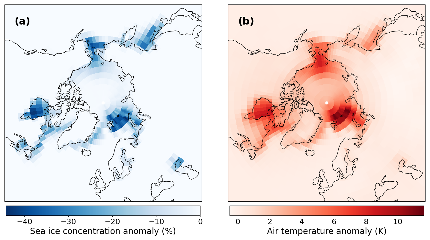
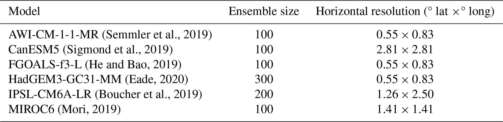
Figure 1 DJF multi-model-mean difference in (a) SIC and (b) near-surface air temperature between present-day and future PAMIP experiments.

The largest reductions in sea ice between the present-day and future experiment are over Hudson Bay, the Sea of Okhotsk, and the Barents and Bering seas (Fig. 1a), resulting in the largest near-surface air temperature anomalies in these regions (Fig. 1b).

2.2 Observation-based datasets

Daily zonal wind speed data from the ERA5 reanalysis (Hersbach et al., 2020) are used to assess the performance of the PAMIP models. ERA5 was re-gridded to a common 2.81°×2.81° resolution for consistency with the PAMIP models. Jet features were calculated for all winters over the period 1979–2020.

2.3 Feature-based jet identification

This study applies a new feature-based approach for diagnosing the low-level North Atlantic jet stream (Perez et al., 2024), with the aim of characterising the association of the jet structure with sea ice loss in more detail than previous studies. A common first step for diagnosing the eddy-driven jet stream is to take the average zonal wind speed across a longitudinal sector. The method applied in this work starts from the non-averaged zonal wind field at 850 hPa (U₈₅₀) (Madonna et al., 2017; Woollings et al., 2010). The wind field is constrained to the North Atlantic sector (15–75° N, 0–60° W) and the winter season (December, January, February (DJF)). A 10 d low-pass Lanczos filter with a window of 61 d is applied to remove short-timescale fluctuations and for closer comparison with previous methods (Woollings et al., 2010), though this choice does not significantly alter the daily jet statistics (Perez et al., 2024).

The feature-based approach identifies westerly jets by using a minimum zonal wind threshold of 8 m s⁻¹. To capture large-scale, zonally oriented jets, a minimum geodesic jet length of 1661 km and a minimum longitudinal extent of 20° are also applied. The latter two thresholds ensure the jet objects identified are zonally orientated and also allow for days with no well-defined jet to be identified. Firstly, the grid point with the maximum U₈₅₀ above the 8 m s⁻¹ threshold is located. Secondly, all surrounding grid points with U₈₅₀ greater than 8 m s⁻¹ are connected to create an outline of the jet object (Fig. 2). The process for identifying a jet object can then be repeated for the next largest U₈₅₀ above the threshold, allowing multiple jet objects to be identified on a single day.

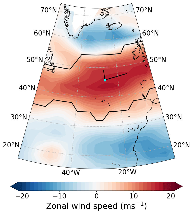
Figure 2 Application of the jet identification method to U₈₅₀ in the North Atlantic region on an example day. The black contour shows the outline of the jet object found on this day, and the blue dot shows the centre of mass of the object giving the jet position, with the minor and major axes denoted by the black lines.

2.3.1 Spatial-moment analysis

Once a jet object has been identified, morphological jet features are determined using spatial-moment analysis. Moments and centralised moments of the U₈₅₀ (λ, ϕ) field are calculated over a two-dimensional object (R) using Eqs. 1 and 2, respectively:

$$\begin{array}{}\text{(1)}& {\displaystyle }{M}_{pq}=\int \underset{R}{\int }{\mathit{\lambda }}^p{\mathit{\varphi }}^q{U}_{\mathrm{850}}\left(\mathit{\lambda },\mathit{\varphi }\right)\mathrm{d}A\text{(2)}& {\displaystyle }{\stackrel{\mathrm{̃}}{M}}_{pq}=\int \underset{R}{\int }{\left(\mathit{\lambda }-\stackrel{\mathrm{‾}}{\mathit{\lambda }}\right)}^p{\left(\mathit{\varphi }-\stackrel{\mathrm{‾}}{\mathit{\varphi }}\right)}^q{U}_{\mathrm{850}}\left(\mathit{\lambda },\mathit{\varphi }\right)\mathrm{d}A,\end{array}$$

where p is the order of the moment in the longitudinal direction and q the order in the latitudinal direction.

The latitude of the jet centre of mass ($\stackrel{\mathrm{‾}}{\mathit{\varphi }}$) is calculated using Eq. (3):

$$\begin{array}{}\text{(3)}& \stackrel{\mathrm{‾}}{\mathit{\varphi }}={\displaystyle \frac{M_{\mathrm{01}}}{M_{\mathrm{00}}}},\end{array}$$

where M₀₀ is the jet mass. The jet speed (U_mean) is the average wind across the jet object and is defined by Eq. (4):

$$\begin{array}{}\text{(4)}& U_{\mathrm{mean}}={\displaystyle \frac{M_{\mathrm{00}}}{{\int }_R\mathrm{d}A}}.\end{array}$$

Finally, jet tilt (α) is the angle between the longitudinal axis and the major axis of the jet and is calculated using Eq. (5):

$$\begin{array}{}\text{(5)}& \mathit{\alpha }={\displaystyle \frac{\mathrm{1}}{\mathrm{2}}}{\tan }^{-\mathrm{1}}\left({\displaystyle \frac{\mathrm{2}{\stackrel{\mathrm{̃}}{M}}_{\mathrm{11}}}{{\stackrel{\mathrm{̃}}{M}}_{\mathrm{20}}-{\stackrel{\mathrm{̃}}{M}}_{\mathrm{02}}}}\right).\end{array}$$

Two-dimensional moment analysis has been applied in previous studies to characterise the stratospheric polar vortex (Waugh, 1997), particularly to assess vortex variability (Lawrence and Manney, 2018; Hall et al., 2021) and to distinguish between split and displacement events (e.g. Mitchell et al., 2013; Maycock and Hitchcock, 2015). Feature-based methods for characterising the jet stream have been applied previously to reanalysis (Limbach et al., 2012; Spensberger and Spengler, 2020). However, those studies focus on the upper-level jet structure rather than the lower-tropospheric component, which is the focus of this study.

2.4 Statistical methods

The initial analysis uses the jet latitude, speed, mass, tilt and area for the largest-mass jet object on each day. The significance of the difference in sample means and cumulative distribution functions was assessed using a two-sample Student t test and Kolmogorov–Smirnov (K–S) test at the 95 % confidence level. Prior to computing the t test and K–S test p values, the effective number of degrees of freedom in the data was determined, where the effective degrees of freedom (N_eff) is defined as

$$\begin{array}{}\text{(6)}& N_{\mathrm{eff}}=N{\displaystyle \frac{\mathrm{1}-r}{\mathrm{1}+r}},\end{array}$$

where N is the sample size, and r is the lag-1 autocorrelation.

This process accounts for autocorrelation in the jet variables at daily timescales and results in a reduced number of independent data points relative to the total sample size. For models that show a significant difference in daily mean and cumulative distribution function (i.e. a significant p value for the t test and K–S test), the difference in mean was subtracted from the future distribution and the K–S statistics recalculated. This process allowed an evaluation of whether differences in the distribution could be explained by a change in the mean or whether higher-order moments such as variance and skewness also contribute to the difference.

We compare standard deviations between time periods to determine the effect of Arctic sea ice loss on the daily and interannual variability in jet features. We also calculate the skewness of the jet features to highlight any asymmetry in the distributions. To determine whether the difference in standard deviations is significant, outputs from present-day and future simulations were bootstrapped with replacement and the difference in their standard deviation calculated. The difference in standard deviation was considered significant if it fell outside the 95th percentile of the bootstrapped differences. For interannual variability, the winter mean for each simulation was bootstrapped, and the standard deviation of the resampled means was calculated. The difference between the present-day and future simulations was then taken to determine the range of interannual variability.

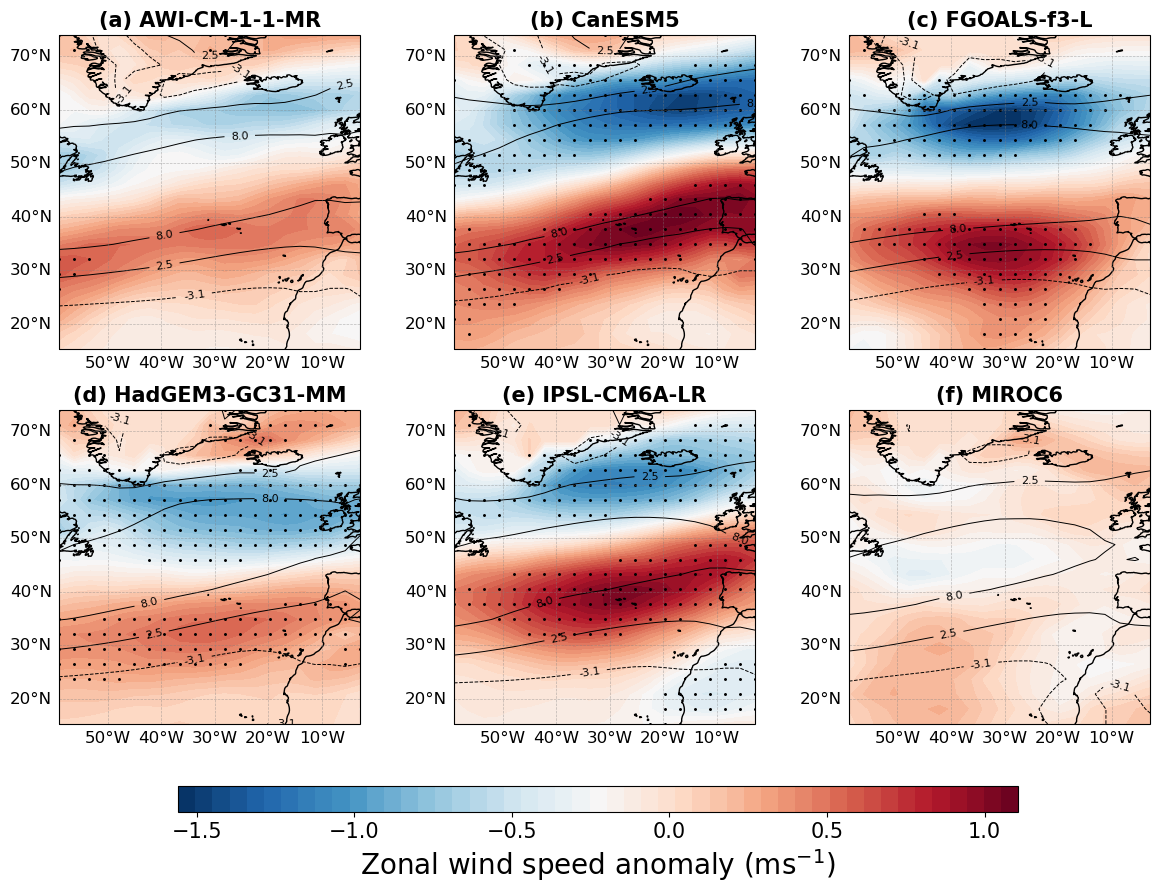
Figure 3 DJF ensemble-mean U₈₅₀ anomaly in selected PAMIP models between simulations forced by present-day and future SIC. Stippling indicates grid points where the difference is significant based on a two-sample Student t test at the 95 % confidence level. Black contours signify the present-day winter U₈₅₀ climatology at 5 ms⁻¹ intervals, with dashed lines showing negative values.

3 Results

3.1 Effect of Arctic sea ice loss on winter-mean circulation

The winter-mean North Atlantic U₈₅₀ anomaly due to future Arctic sea ice loss is shown in Fig. 3. CanESM5, FGOALS-f3-L, HadGEM3-GC31-MM and IPSL-CM6A-LR show a decrease in wind speed at 50–60° N and an increase near 30–40° N (Fig. 3b–e), corresponding to an equatorward jet shift. AWI-CM-1-1-MR shows a similar response to HadGEM3-GC31-MM, but the difference is non-significant, potentially because of the smaller ensemble size (Table 1). MIROC6 shows a very weak and non-significant U₈₅₀ response, which is consistent with the weak JLI response in MIROC6 found by Ye et al. (2023).

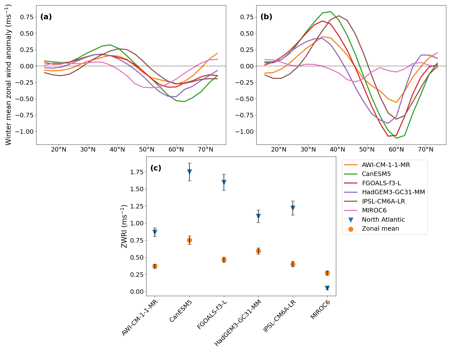
Figure 4 DJF mean U₈₅₀ anomaly due to Arctic sea ice loss in PAMIP models for (a) zonal mean (0–360°) and (b) North Atlantic (0–60° W) mean. Note the different vertical scales in (a) and (b). (c) The ZWRI of Smith et al. (2022) for the zonal mean (yellow circles) and North Atlantic sector (blue triangles).

Smith et al. (2022) found a winter-mean equatorward jet shift due to Arctic sea ice loss in the PAMIP models based on the hemispheric zonal-mean zonal wind. However, changes in hemispheric zonal winds may not reflect the local North Atlantic eddy-driven jet response. Therefore, in Fig. 4 we compare the zonal-mean U₈₅₀ differences (Fig 4a) and the North Atlantic sector (0–60° W) U₈₅₀ differences (Fig. 4b). In both cases a dipole pattern is evident, with positive U₈₅₀ at lower latitudes and negative U₈₅₀ differences at higher latitudes, corresponding to an equatorward jet shift. However, for all models except MIROC6, the North Atlantic sector U₈₅₀ differences are larger than the zonal-mean U₈₅₀ differences. This can be further seen by examining the zonal wind response index (ZWRI) from Smith et al. (2022), calculated as the difference in vertically averaged (600–150 hPa) zonal-mean zonal wind between two latitude bands (30–39 and 54–63° N). We recalculate this for the North Atlantic sector only (0–60° W) (Fig. 4c). Note that, in contrast to Smith et al. (2022), we use U₈₅₀ for both calculations for consistency.

For five of the six PAMIP models analysed, the ZWRI for the North Atlantic sector is greater than for the zonal mean, with the response in five models being 0.5–1 ms⁻¹ (around a factor of 2–3) larger. Thus, the overall weak zonal-mean ZWRI identified by Smith et al. (2022) is, on average, associated with a stronger local equatorward jet shift in the North Atlantic, with the exception of MIROC6, which shows a weaker response in the North Atlantic than in the zonal mean. This demonstrates that it is important to examine the regional response to Arctic sea ice loss in individual basins. The ZWRI mainly reflects a jet latitude shift. The Euler-based North Atlantic jet strength calculated from the sector-average DJF zonal wind profiles shows generally non-significant changes, except for HadGEM3-GC31-MM, which has a small jet weakening (−0.33 ± 0.25 ms⁻¹). To explore a possible origin of the different ZWRI in models, we investigated the relationship between meridional temperature gradient changes due to sea ice loss around the high- and low-latitude nodes of the ZWRI, respectively. For the high-latitude ZWRI node, there was no apparent relationship between wind speed and temperature gradient changes across models. The result for the low-latitude ZWRI node suggested that models which show a strengthening of North Atlantic zonal wind speed have a weaker change in meridional temperature gradient (not shown); however, confirming whether such a relationship is robust would require analysis of a larger sample of models.

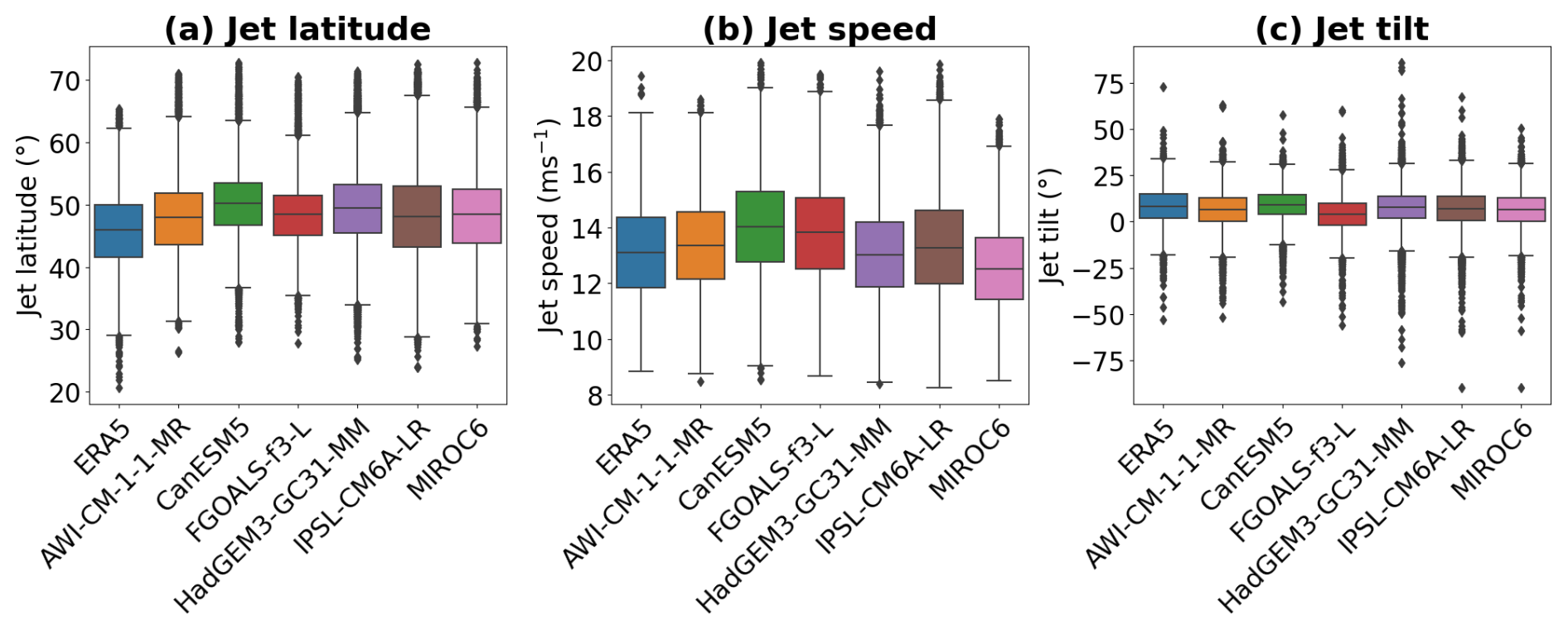
Figure 5 Distribution of daily jet features for present-day PAMIP models compared with ERA5 reanalysis. Comparisons shown are for (a) jet latitude, (b) jet speed and (c) jet tilt. Coloured boxes show the interquartile range; the horizontal line shows the median; and the whiskers show the overall distributions, with diamonds representing outliers.

3.2 Model performance for climatological jet structure

Before analysing the changes in jet characteristics under future sea ice loss, we first compare the present-day SIC PAMIP experiments with ERA5 for daily jet latitude, speed and tilt (Fig. 5). The comparison is not perfect because the PAMIP models do not include any year-to-year variation in boundary conditions that will contribute to variability in ERA5, but it gives an indication of their capability.

All PAMIP models show a climatological poleward bias in jet latitude, with a multi-model-mean difference of 2.6° compared to ERA5. A similar poleward bias in the North Atlantic jet has been previously shown for CMIP5 models using the JLI (Iqbal et al., 2018). ERA5 jet speed and jet tilt largely lie within the PAMIP model spread, with differences between the multi-model mean and reanalysis of 0.1 ms⁻¹ for jet speed and −1.3° for jet tilt. This analysis indicates that PAMIP models generally perform well for characterising the present-day jet morphology, but the differences should be considered when interpreting model results.

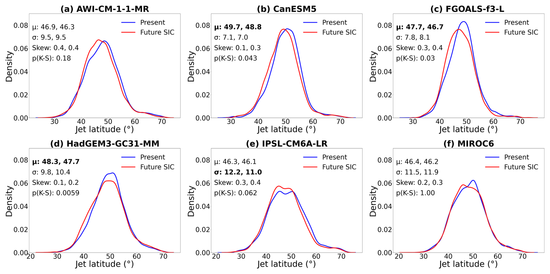
Figure 6 Distributions of daily jet latitude in winter for simulations forced by present-day (blue) and future (red) SIC. Data are for the largest-mass jet object on each day, and distributions have been fitted with a kernel density estimate. The ensemble mean (μ), standard deviation (σ), skew and K–S test p value for the distributions are shown in the legend, with present-day statistics (left) and future statistics (right). Means are bold where the difference between present-day and future simulations is statistically significant based on a t test at the 95 % confidence level. Standard deviations are bold where the difference between time periods is greater than for random sampling.

3.3 Effect of Arctic sea ice loss on daily jet morphology

3.3.1 Jet latitude ($\stackrel{\mathrm{‾}}{\mathit{\varphi }}$)

Distributions of jet latitude of the largest-mass jet object on each winter day are shown in Fig. 6. The jet shifts equatorward in the CanESM5, FGOALS-f3-L and HadGEM3-GC31-MM models between present-day and future simulations (Fig. 6b–d), with a mean equatorward shift in these models of 0.8 ± 0.1°. The mean equatorward shift across all models was 0.6 ± 0.1°. Removing the mean difference from the future distribution results in a non-significant p value for the K–S test, which shows that the overall differences in jet latitude distributions can be explained by a change in mean. For the AWI-CM-1-1-MR, IPSL-CM6A-LR and MIROC6 models, the difference in mean jet latitude is non-significant (Fig. 6a, e, f). Although IPSL-CM6A-LR shows a significant equatorward shift in the winter-mean zonal wind speed response to Arctic sea ice loss (Fig. 4b), application of the feature-based daily jet identification method indicates a non-significant change to jet latitude. However, the change is close to statistical significance, with a p value of 0.06. AWI-CM-1-1-MR shows a similar mean decrease in jet latitude to HadGEM3-GC31-MM, but the difference is not significant, potentially due to the smaller ensemble size.

Distributions of jet latitude in the present-day SIC experiment are positively skewed and generally become more positively skewed with future SIC. IPSL-CM6A-LR shows a small but significant reduction of −1.2° in daily jet latitude standard deviation between the present and future, but for all other models the change in variability is non-significant. In contrast, four models show a significant change in interannual jet latitude variability. However, the sign of the response is not consistent across models, with AWI-CM-1-1-MR and MIROC6 showing an increase, while CanESM5 and IPSL-CM6A-LR show a decrease. Key statistics for jet latitude in each model simulation are summarised in Table S1 in the Supplement.

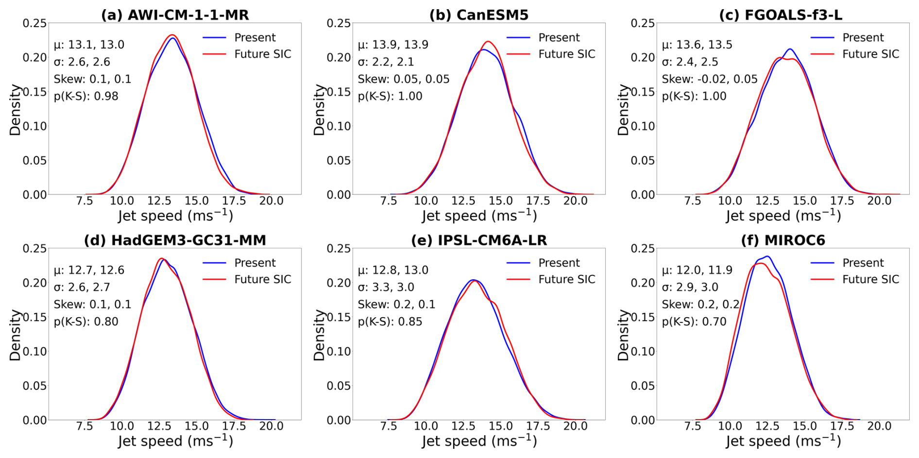
Figure 7 Distributions of daily jet speed in winter for simulations forced by present-day (blue) and future (red) SIC. Data are for the largest-mass jet object on each day, and distributions have been fitted with a kernel density estimate. The ensemble mean (μ), standard deviation (σ), skew and K–S test p value for the distributions are shown in the legend, with present-day statistics (left) and future statistics (right).

3.3.2 Jet speed (U_mean)

Distributions of jet speed for the largest-mass jet object on each winter day are shown in Fig. 7. The distributions show no significant change between present-day and future SIC experiments for all models, while previous studies have highlighted a weakening of jet speed with sea ice loss (Smith et al., 2022; Ye et al., 2023). However, in these studies the jet speed response is weak and lacks statistical significance across models. It is interesting that while the winter-mean and North Atlantic sector-mean ZWRI shows a strengthening in several models (Fig. 4c), this increase is not found when taking a view centred on daily jet objects. The daily variability in jet speed is not significantly different between simulations for all models, while four models do exhibit a notable shift in interannual variability. However, this difference is not consistent across models, with AWI-CM-1-1-MR and MIROC6 showing an increase, while FGOALS-f3-L and HadGEM3-GC31-MM show a decrease. It is also noted that the models indicating a significant alteration in jet speed interannual variability do not align with those showing significant changes in jet latitude interannual variability. Key statistics for jet speed are summarised in Table S2.

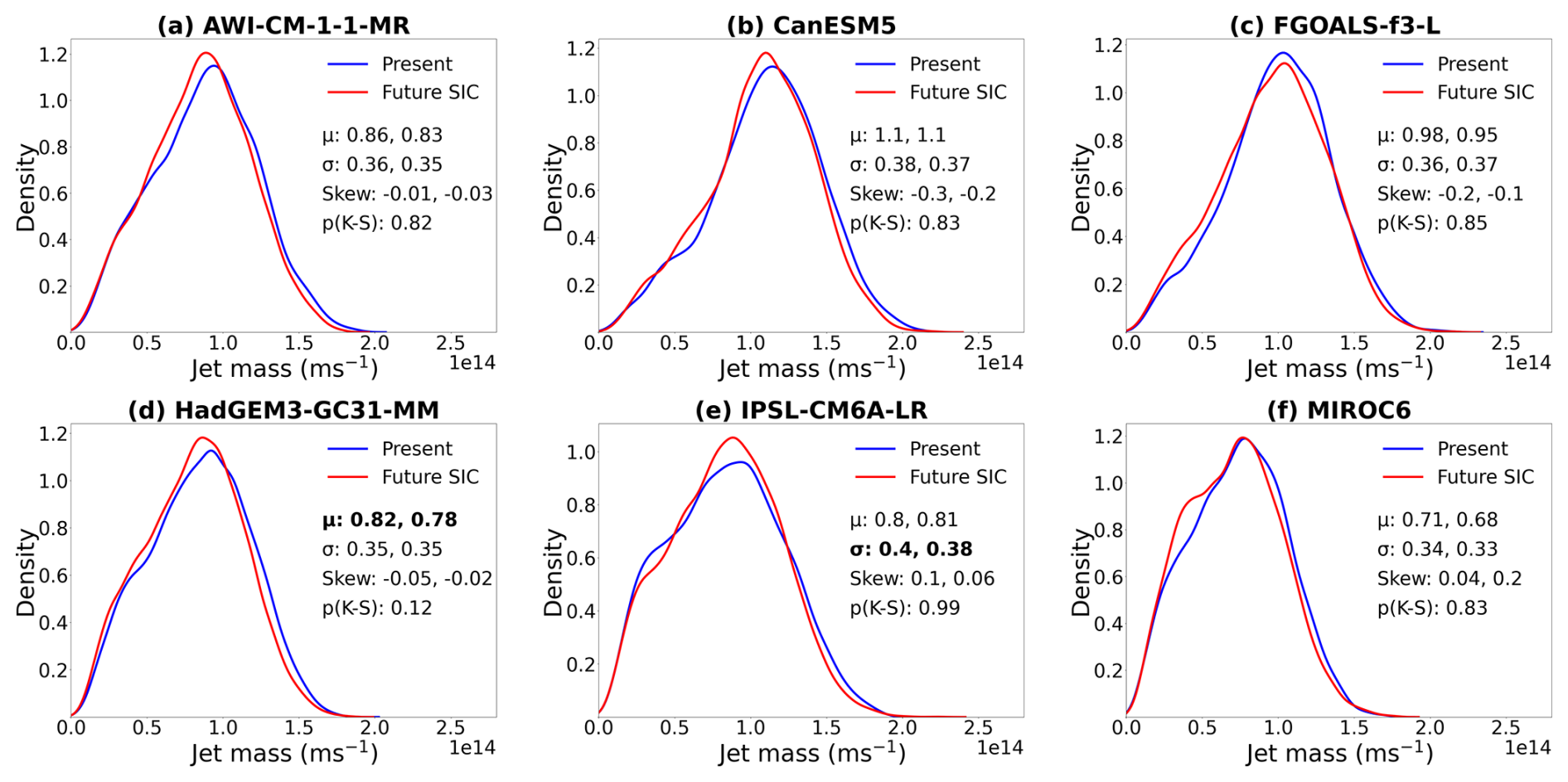
Figure 8 Distributions of daily jet mass in winter for simulations forced by present-day (blue) and future (red) SIC. Data are for the largest-mass jet object on each day, and distributions have been fitted with a kernel density estimate. The ensemble mean (μ), standard deviation (σ), skew and K–S test p value for the distributions are shown in the legend, with present-day statistics (left) and future statistics (right). The ensemble mean and standard deviation have been scaled by a factor of 1×10¹⁴ for clarity. Means are bold where the difference between present-day and future simulations is statistically significant based on a t test at the 95 % confidence level. Standard deviations are bold where the difference between time periods is greater than for random sampling.

3.3.3 Jet mass (U_mass) and tilt (α)

Distributions of jet mass for the largest-mass jet objects on each winter day are shown in Fig. 8. There is no significant difference in jet mass or its daily variability between present-day and future SIC experiments for five of the six models. One exception is that HadGEM3-GC31-MM shows a significant difference in mean but no difference in the distribution when assessed using a K–S test. The significant, but rather modest, difference in mean may be caused by the HadGEM3-GC31-MM's larger ensemble size compared to the other models. Furthermore, IPSL-CM6A-LR shows no significant difference in mean but a significant difference in jet mass daily variability.

Three models show a significant change in jet mass interannual variability, but as for jet latitude and speed, the sign of the change is not consistent across models. Although the difference between simulations is not significant, for some models the shape of the distribution suggests a decrease in jet mass. Plotting the distribution of daily jet area (Fig. S1 in the Supplement) shows that changes in the jet mass follow changes in area. This suggests that differences in the distribution of wind within the jet are not important for the differences in jet mass, and instead the differences are dominated by a change in jet area. Key statistics are summarised in Table S3 for jet mass and Table S4 for jet area.

Finally, the jet identification method extracts the jet tilt. As with jet speed and jet mass, there is no significant change in daily jet tilt across models. Distributions of daily jet tilt are shown in Fig. S2, and key statistics are summarised in Table S5. We find that the climatological-mean daily jet tilt ranges from 4–9° across models, with no significant difference in daily or interannual variability under future Arctic sea ice forcing.

While the diagnostics were calculated with re-gridded U₈₅₀ data to ensure consistency, we have tested the results using the native grid for the highest-horizontal-resolution model (AWI-CM-1-1-MR; 0.55° latitude × 0.83° longitude) and find that this does not significantly alter the results (Fig. S4). Jet diagnostics were also calculated in each month to assess differences from the winter average. In AWI-CM-1-1-MR, mean jet latitude shifts significantly in December and January, and variability increases in February, though these changes are not evident in the winter mean. For CanESM5, jet tilt significantly decreases in February, which is absent in the winter mean. In other models, month-specific changes align with the winter mean. However, winter-mean shifts in jet latitude for CanESM5, FGOALS-f3-L and HadGEM3-GC31-MM and reduced variability in IPSL-CM6A-LR are not seen in individual months. These differences are likely due to limited monthly sample sizes.

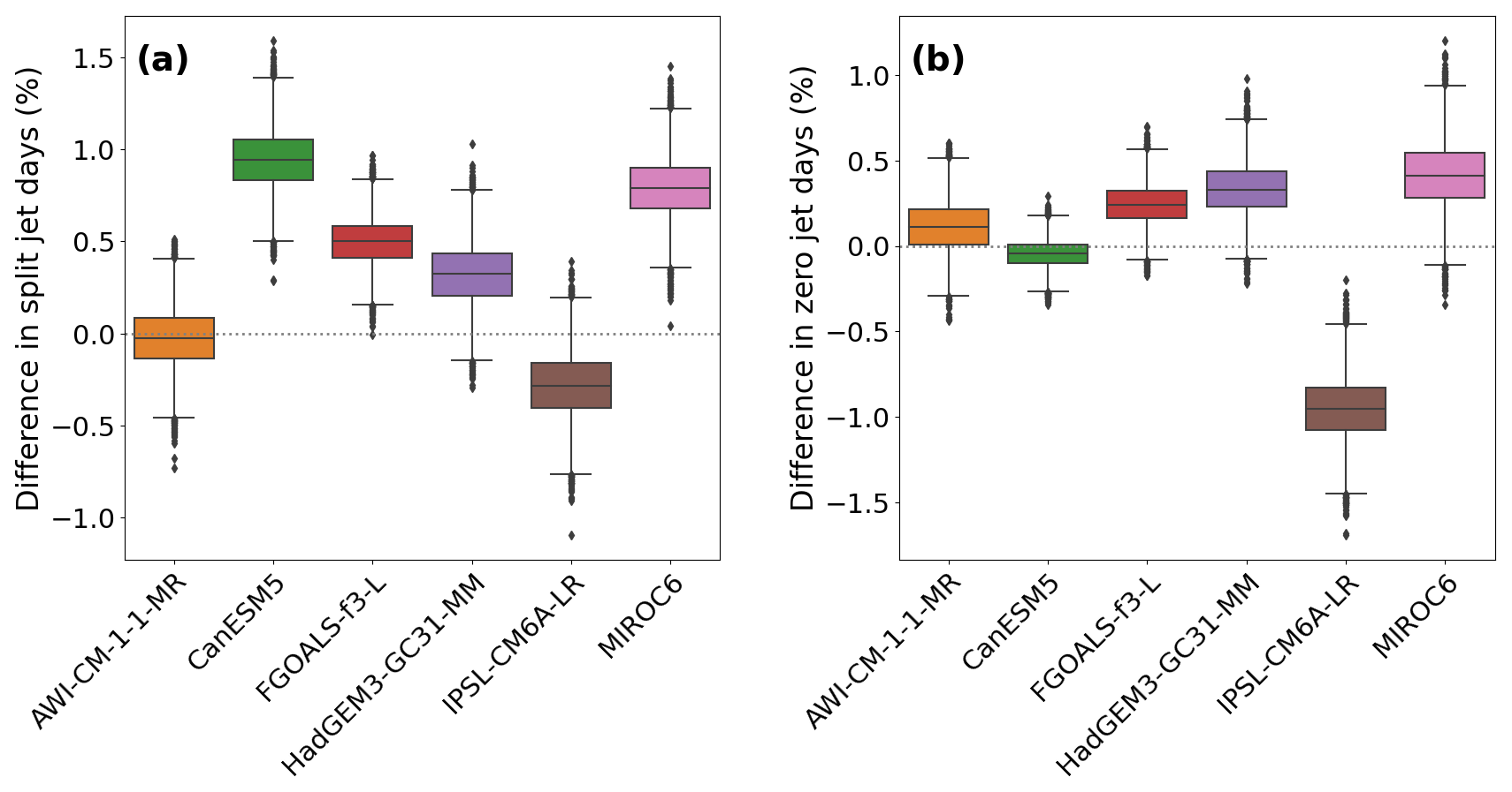
Figure 9 Difference in the occurrence of split-jet and zero-jet days between present-day and future simulations. The percentages of (a) split- and (b) zero-jet days are shown between bootstrap resamples of present-day and future ensembles. Coloured boxes show the first quartile, median and third quartiles of the differences, whiskers show the overall distributions, and black diamonds represent outliers.

3.4 Occurrence of split-jet and zero-jet days

The occurrence of split-jet and zero-jet days in present-day and future simulations was quantified to further explore changes in jet morphology (Fig. 9). Split-jet days are defined as days when two jet objects are identified, while zero-jet days are days when no jet is identified. We sum the occurrence of split-jet days over all ensemble members and take the difference between simulations. To assess the significance of the difference, we generate bootstrapped samples of both simulations, calculate the occurrence of split-jet days in each and take the difference. The spread of the difference in the occurrence of split-jet days between present-day and future simulations in bootstrapped samples is shown in Fig. 9a. A difference in split-jet days is considered significant where the spread does not encompass zero. The same process was followed to assess the number of zero-jet days (Fig. 9b).

The present-day multi-model-mean percentage of split-jet days is 3 %. The CanESM5, FGOALS-f3-L and MIROC6 models show a small but significant increase in the frequency of split-jet days of around 0.5 %–1 % between present-day and future simulations. We also assess the significance in the change in frequency of split-jet days by evaluating the impact on jet latitude, as a significant increase in split-jet days may result in broadening of the jet latitude distribution, due to the increased instances of low- and high-latitude jets. There are no significant differences in standard deviation between the simulations when the second jet objects are included in distributions of daily jet latitude (Fig. S3). While significant differences in split-jet days are found in some models, the proportion of sample days the change represents is small (<1.5 %), which makes the impact on the overall distribution modest. The occurrence of zero-jet days shows no significant change between the present day and the future for five of the six models. However, IPSL-CM6A-LR shows a significant decrease in zero-jet days.

4 Discussion and conclusions

This study set out to characterise the effects of projected future Arctic sea ice loss on the winter North Atlantic jet stream morphology. We have assessed how daily jet features are altered by sea ice loss by analysing daily zonal wind speed data from the Polar Amplification Model Intercomparison Project (PAMIP), which provides simulations of climate forced by present-day and future sea ice concentrations. While previous studies have been limited to a zonally or sectorally averaged, one-dimensional assessment of the jet (Smith et al., 2022; Ye et al., 2023), this analysis has given a more detailed view of the North Atlantic jet morphology by characterising additional jet features. As such, a new feature-based method, which does not rely on averaging over a longitudinal sector, was used to quantify changes in jet latitude, speed, tilt, mass and area. The analysis also goes beyond a study of seasonal-average changes in the jet stream by assessing the effect of Arctic sea ice loss on daily jet feature variability and the frequency of split jets.

The significant equatorward jet shift shown by some models is consistent with the winter zonal-mean perspective (Smith et al., 2022). Likewise, the multi-model-mean shift in daily jet latitude was $-\mathrm{0.6}\pm \mathrm{0.1}\mathit{°}$, which is the same as the multi-model winter-mean change found by applying the JLI to a larger set of PAMIP models (Ye et al., 2023). Three models show a significant change in daily mean jet latitude (Fig. 6) compared with four models showing a significant change based on the winter-mean zonal wind speed (Fig. 3). The lack of a stronger, more statistically significant response for daily jet latitude in IPSL-CM6A-LR (p value =0.06) may be due to larger daily variability in the jet than seasonal variability. IPSL-CM6A-LR also shows a decrease in the occurrence of zero-jet days (Fig. 9b) captured by the jet identification method. Removing zero-jet days results in a non-significant difference in standard deviation between the simulations compared to the range of standard deviations from random sampling. This suggests that the significant decrease in jet latitude daily variability for IPSL-CM6A-LR is due to the decrease in zero-jet days.

The feature-based jet identification method allows for the quantification of split-jet days, a detail that is missing from previous studies. Three of the six PAMIP models show an increase in split-jet days with future Arctic sea ice loss. However, the increase is relatively small (<1.5 %), meaning the total standard deviation of daily jet latitude is not affected. Split jets are often characterised by one high-latitude and one low-latitude jet object. Therefore, a larger increase in split-jet days between the present and future could lead to a broadening of the jet latitude distribution. We find that including the second-largest jet object to capture the split jets has a minimal effect on the difference in the standard deviation and skewness of daily jet latitude between the present and future sea ice simulations (Fig. S3). Although split-jet days make up a small percentage of days overall, it is important to quantify them because they can be associated with blocked flow, resulting in more persistent and sometimes extreme winter weather in Europe. Further work could analyse jet splitting in different seasons using this jet identification method given the known links with summer heatwaves (Rousi et al., 2022).

The results suggest that Arctic sea ice loss has no effect on North Atlantic jet speed, which contradicts the argument that Arctic sea ice loss will drive a weaker jet stream in the future (e.g. Outten and Esau, 2012; Francis and Vavrus, 2015). Furthermore, this result does not align with the zonal-mean perspective, which indicates a robust weakening of westerly winds across all PAMIP models (Smith et al., 2022). Minimal influence on jet speed across all models also contrasts with the JLI approach, which shows alterations in jet speed for HadGEM3-GC31-MM, IPSL-CM6A-LR and MIROC6, albeit with some models showing a strengthening of the jet and others showing a weakening (Ye et al., 2023). This analysis highlights that the result for jet speed is dependent on the approach for characterising the jet.

Jet mass represents the area-weighted jet speed. Therefore, models that exhibit an equatorward jet shift and no change in jet speed (CanESM5, FGOALS-f3-L and HadGEM3-GC31-MM) might be expected to show an increase in jet mass due to an increase in the jet area owing to the Earth's curvature. However, none of the models show a significant change in mean jet mass. Some models appear to show a slight decrease in jet mass and jet area with future sea ice loss (Figs. 8 and S1), but the differences are not significant.

Jet tilt is an aspect that has been neglected in the zonal-mean perspective of previous studies. However, the results show no significant changes in jet tilt between present-day and future sea ice simulations. A wavier jet may be expected to occur alongside higher-amplitude variations in jet tilt, but this is not seen, which suggests that the jet waviness theory (Francis and Vavrus, 2015; Petoukhov et al., 2013) is not supported by PAMIP simulations.

The total variability as measured by the standard deviation shows no significant changes in daily variability and inconsistent changes in interannual variability for all jet features between present-day and future simulations. The modelled differences in jet features are all smaller than the present-day interannual variability, which is consistent with previous studies focusing on latitude and speed (Smith et al., 2022; Ye et al., 2023). The absence of changes in standard deviation of jet parameters does not rule out the possibility for other changes in North Atlantic circulation that are not detected by this measure. For example, there could be changes in the frequency and/or persistence of certain weather regimes which may have compensating effects when viewed through the standard deviation. In future work, we will examine the relationship between the jet parameters and weather regime frameworks (e.g. Madonna et al., 2017).

The analysis in this study is limited to an atmosphere-only diagnosis of the jet response to Arctic sea ice loss. The jet response may also be influenced by atmosphere–ocean coupling (Deser et al., 2015) and ice–ocean–atmosphere coupling (Strommen et al., 2022), which may not be well represented in models. However, this analysis is beyond the scope of this study. While there are some coupled atmosphere–ocean sea ice perturbation experiments in PAMIP, they did not provide daily frequency output needed for this study. Furthermore, we were only able to use a subset of PAMIP models that provided daily zonal wind speed data for the atmosphere-only experiments. A further caveat is the potential role of the signal-to-noise problem, which may affect simulations of the North Atlantic atmospheric response to Arctic sea ice loss (Smith et al., 2022). This effect may mean the modelled changes in the jet are an underestimation, despite the use of large ensembles in PAMIP simulations. It is also possible that an ensemble size of 100 members is not large enough to separate the signal from internal variability (Ye et al., 2024). Nevertheless, the analysis of high-frequency jet variability is important given the hypothesised links to extreme weather events. The model results presented here do not support a strong role for Arctic sea ice loss in driving increased jet variability and associated extreme events in boreal winter.