Physical processes leading to extreme day-to-day temperature change – Part 1: Present-day climate

Extreme temperature changes from one day to another that are associated with either warming or cooling can have a significant impact on health, the environment, and society. Previous studies have shown that such day-to-day temperature (DTDT) changes are typically more pronounced in the extratropics than the tropics. However, the underlying physical processes and the relationship between extreme events and the large-scale atmospheric circulation remain poorly understood. Here, these processes are investigated for different locations around the globe based on ERA5 reanalysis data and Lagrangian backward-trajectory calculations. We show that extreme DTDT changes in the extratropics are generally associated with changes in air mass transport, particularly shifts from warmer to colder air parcels or vice versa that are linked to regionally specific synoptic-scale circulation anomalies (ridge or trough patterns). These dominant effects of advection are modulated by changes in adiabatic and diabatic processes in the transported air parcels, which either amplify or dampen DTDT decreases (cooling events) and increases (warming events) depending on the region and season. In contrast, extreme DTDT changes during December–February in the tropics are controlled by local processes rather than changes in advection. For instance, the most significant DTDT decreases are associated with a shift from less cloudy to more cloudy conditions, highlighting the crucial role of solar radiative heating. The mechanistic insights into the extreme DTDT changes obtained in this study can help improve the prediction of such events and anticipate future changes in their occurrence frequency and intensity, which will be investigated in part 2 of this study.

1 Introduction

Day-to-day temperature (DTDT) changes, here represented by temperature differences between consecutive days, can have significant implications across various sectors, including the economy, ecology, and human health (Gough, 2008; Zhou et al., 2020; Kotz et al., 2021; Hovdahl, 2022). A change in DTDT variation is linked to increased mortality rates, with the impact varying across geographic regions such as the northern latitudes, tropics, and southern latitudes (Chan et al., 2012; Hovdahl, 2022; Sarmiento, 2023; Wu et al., 2022a). A recent study further reveals that temperature changes can impact heat-related mortality regionally by more than 7 % of total deaths (Wu et al., 2022b). High DTDT variation has a negative effect on economic activity (Linsenmeier, 2023), with economic losses exhibiting regional disparities, as a 1 °C increase in DTDT change results in an increase of 3 %–5 % in vulnerability in midlatitude and high-latitude areas but more than 10 % in low-latitude and coastal regions (Kotz et al., 2021). These previous studies highlight the critical need for comprehensive studies investigating DTDT variation and the underlying atmospheric processes in the present climate.

With regard to long-term trends in DTDT change, an early study by Karl et al. (1995) observed a decrease at midlatitude to high-latitude stations, particularly during the summer season, while no significant trend was detected in Australia. Recently, Xu et al. (2020) extended these results by demonstrating a substantial increase in summer DTDT change across diverse regions such as the Arctic coast, southern China, and Australia but a decreasing winter DTDT change in the midlatitudes to high latitudes. These trends align with the comprehensive analysis by Krauskopf and Huth (2024) and Wan et al. (2021), attributing spatiotemporal fluctuations in global temperature variability, except during boreal summer, to anthropogenic influences. Although most prior investigations have predominantly focused on analyzing trends in the average magnitude of DTDT change, it is equally important to understand extreme DTDT changes. The concept of extreme DTDT events, characterized by daily average temperature changes larger than ±10 °C, has been introduced in a recent study that only focused on the midlatitudes to high latitudes (Zhou et al., 2020). Since higher DTDT variation is observed in the northern midlatitudes to high latitudes, spanning regions such as northern Asia, the United States, and Europe (Gough, 2008; Xu et al., 2020), we can also expect more pronounced extreme DTDT changes in these regions compared to in the lower latitudes (Fig. 2a–d), which is consistent with the findings of Zhou et al. (2020). Here, to account for such regional differences and to investigate extreme DTDT changes globally, we utilize percentile-based thresholds that are widely used to identify temperature extremes (Bieli et al., 2015; Pfahl, 2014; Nygård et al., 2023).

The relationship between daily temperature extremes (extremely high or low temperature, not extreme DTDT changes) and distinct circulation patterns at global and regional scales has been thoroughly investigated (Horton et al., 2015; Adams et al., 2021; Nygård et al., 2023; Pfahl, 2014). For example, in Europe, extreme warm events in summer often coincide with blocking anticyclones or subtropical ridges, while winter cold extremes are linked to North Atlantic blocking, facilitating the intrusion of cold air masses (Nygård et al., 2023; Kautz et al., 2022; Pfahl and Wernli, 2012; Sillmann et al., 2011). Similarly, warm extremes in North America correlate with anticyclonic circulation and ridges, whereas extreme cold is linked to troughs and advection of continental air masses (Adams et al., 2021; Wang et al., 2019). Frontal structures are key drivers of DTDT variability (Ghil and Lucarini, 2020), and the relevance of fronts for European DTDT extremes has been confirmed in the detailed study by Piskala and Huth (2020). Further, particular insights into the physical processes associated with daily temperature extremes have been obtained from Lagrangian studies based on air parcel trajectory analyses, which have quantified the contributions of advection, adiabatic, and diabatic heating/cooling to temperature extremes (Schumacher et al., 2019; Bieli et al., 2015; Röthlisberger and Papritz, 2023b, a; Zschenderlein et al., 2019; Hartig et al., 2023). All these studies highlight the significance of specific circulation anomalies in causing extreme weather in the midlatitudes to high latitudes. In contrast, tropical regions generally experience much weaker temperature advection compared to the extratropics, and extreme-temperature events there are more strongly influenced by local processes such as precipitation, radiation, cloud cover, and surface fluxes (Gough, 2008; Matuszko et al., 2004; Sun and Mahrt, 1995; Dirmeyer et al., 2022). Nevertheless, accelerated warming of extreme temperatures across tropical land has been observed recently (Byrne, 2021). These previous studies have established the groundwork for understanding the origins of daily temperature extremes, also providing a fundamental basis for deeper investigations into extreme DTDT changes globally.

This paper investigates in detail the influence on extreme DTDT changes of altering air mass properties within the large-scale atmospheric circulation. We use observations and reanalysis data to quantify the magnitude of extreme DTDT changes worldwide. To study the underlying processes, we apply a composite approach and perform a Lagrangian analysis, calculating backward trajectories of surface air masses from selected locations on the 2 d involved in extreme DTDT changes. The contributions of temperature advection and adiabatic and diabatic processes are then quantified following previous studies of temperature extremes (Bieli et al., 2015; Röthlisberger and Papritz, 2023a; Santos et al., 2015; Röthlisberger and Papritz, 2023b; Nygård et al., 2023). We aim to address the following research questions:

1. Which (changes in) atmospheric circulation patterns occur on the consecutive days associated with extreme DTDT changes?

2. Which physical processes contribute to the occurrence of extreme DTDT changes?

2 Data and method

2.1 ERA5

ERA5 is the fifth-generation European Centre for Medium-range Weather Forecasts (ECMWF) global reanalysis product, providing climate and weather data for the past 8 decades. It was developed by 4D-Var data assimilation in cycle CY41R2 of the ECMWF Integrated Forecasting System (Hersbach et al., 2020). It is an updated version of the widely used ERA-Interim reanalysis, employing a newer version of the ECMWF Earth system model with 137 hybrid sigma/pressure levels in the vertical up to 0.01 hPa (Hersbach, 2019). It provides hourly estimates of several atmospheric, ocean wave, and land surface quantities on a regular latitude–longitude grid of 0.25°. Recently, ERA5 data have been used for different climate- and weather-related global and regional studies (Böker et al., 2023; Simmons, 2022), and some have recommended it as the best alternative for regions with sparse observational coverage (Sharma et al., 2020; Sheridan et al., 2020). We use ERA5 data from 1980 to 2020, encompassing global daily mean 2 m surface air temperature (calculated from hourly temperature), total precipitation, and several three-dimensional atmospheric fields (temperature, horizontal and vertical winds, geopotential). The spatial resolution for all analyses is 0.25°×0.25°, except for the trajectory calculations, for which input data at a horizontal resolution of 0.5°×0.5° are employed. The temporal resolution of the near-surface temperature and composite analysis is daily, while the input data for the trajectories have an hourly resolution. We have compared the magnitude of DTDT changes from ERA5 data with observational datasets (HadGHCND and Berkeley Earth Surface Temperatures (BEST)), with a detailed description of the datasets available in the Supplement.

2.2 DTDT variation and extremes

This study defines DTDT change, denoted δ_T, as the difference in daily mean near-surface air temperature between the previous day (T_t−1) and the day of the event (T_t), as shown in Eq. (1).

$$\begin{array}{}\text{(1)}& {\mathit{\delta }}_T=(T_t-T_{t-\mathrm{1}})\end{array}$$

The average daily temperature change, μ_DTDT, reflects the difference between the temperatures at the start (T₀) and end (T_n) of the time series (Eq. 2).

$$\begin{array}{}\text{(2)}& {\mathit{\mu }}_{\mathrm{DTDT}}={\displaystyle \frac{\mathrm{1}}{n}}{\sum }_{t=\mathrm{1}}^n(T_t-T_{t-\mathrm{1}})=T_n-T_{\mathrm{0}}\end{array}$$

To capture typical DTDT changes, we thus use the standard deviation, σ_DTDT, as shown in Eq. (3).

$$\begin{array}{}\text{(3)}& {{\mathit{\sigma }}_{\mathrm{DTDT}}}^{\mathrm{2}}={\displaystyle \frac{\mathrm{1}}{n}}{\sum }_{t=\mathrm{1}}^n(T_t-T_{t-\mathrm{1}}{)}^{\mathrm{2}}\end{array}$$

By inserting the average daily temperature μ_T and expanding the squared term, we find a relationship between σ_DTDT, the standard deviation of the daily mean temperature (σ_T), and the covariance between consecutive days ($\mathrm{COV}(T_t,T_{t-\mathrm{1}})$):

$$\begin{array}{}\text{(4)}& \begin{array}{rl}{\mathit{\sigma }}_{\mathrm{DTDT}}^{\mathrm{2}}& ={\displaystyle \frac{\mathrm{1}}{n}}{\sum }_{t=\mathrm{1}}^n(\left(T_t-{\mathit{\mu }}_T\right)-(T_{t-\mathrm{1}}-{\mathit{\mu }}_T){)}^{\mathrm{2}}\\ & ={\displaystyle \frac{\mathrm{1}}{n}}{\sum }_{t=\mathrm{1}}^n({\left(T_t-{\mathit{\mu }}_T\right)}^{\mathrm{2}}+{\left(T_{t-\mathrm{1}}-{\mathit{\mu }}_T\right)}^{\mathrm{2}}\\ & -\mathrm{2}\left(T_t-{\mathit{\mu }}_T\right)(T_{t-\mathrm{1}}-{\mathit{\mu }}_T))\\ & \approx \mathrm{2}{\mathit{\sigma }}_T^{\mathrm{2}}-\mathrm{2}\mathrm{COV}(T_t,T_{t-\mathrm{1}}).\end{array}\end{array}$$

The approximation in Eq. (4) is based on the fact that, for large n, both $\frac{\mathrm{1}}{n}{\sum }_{t=\mathrm{1}}^n(T_{t-\mathrm{1}}-{\mathit{\mu }}_T{)}^{\mathrm{2}}$ and $\frac{\mathrm{1}}{n}{\sum }_{t=\mathrm{1}}^n(T_t-{\mathit{\mu }}_T{)}^{\mathrm{2}}$ are good estimators of ${\mathit{\sigma }}_T^{\mathrm{2}}$. Finally, the standard deviation of DTDT can thus be expressed as a function of the usual standard deviation (σ_T) and the lag-1 autocorrelation (r_1,T) of daily mean temperature, as shown in Eq. (5).

$$\begin{array}{}\text{(5)}& {\mathit{\sigma }}_{\mathrm{DTDT}}={\mathit{\sigma }}_T\sqrt{\mathrm{2}(\mathrm{1}-r_{\mathrm{1},T})}\end{array}$$

In addition, extreme DTDT changes are studied using the percentile method. Extreme cooling and warming events at each grid box are identified using the 5th and 95th percentiles of the DTDT change distribution as thresholds, respectively. The analyses focus on the two main seasons: December–February (DJF) and July–August (JJA). Accordingly, 184 events in DJF and 188 events in JJA were selected at each location based on the ERA5 dataset.

2.3 Trajectory setup

The Lagrangian analysis tool (LAGRANTO), which was introduced by Sprenger and Wernli (2015), is used to calculate backward trajectories of near-surface air masses on days associated with extreme DTDT changes from 1980 to 2020. The trajectories are initialized at 18:00 UTC on both the preceding day (t−1) and the event day (t) at 10, 30, 50, and 100 hPa above the surface at the corresponding grid cells. Similar to studies on extreme temperatures (Zschenderlein et al., 2019), the different initialization heights are used to sample a near-surface layer that is assumed to be well-mixed. The time difference of 24 h between the two initializations allows for a proper separation of the air masses before and after the temperature change. Although LAGRANTO is used to calculate 10 d backward trajectories, extremes typically develop on a timescale of 2–3 d (Bieli et al., 2015; Röthlisberger and Papritz, 2023a). Therefore, we focus on 3 d backward trajectories for the analysis. Various variables of interest, including latitude, longitude, pressure, temperature, and potential temperature, are interpolated along the trajectory paths and saved at 1 h intervals.

2.4 Lagrangian temperature variability decomposition

To better understand the underlying mechanisms of extreme DTDT changes, our analysis focuses on four specific locations: two grid boxes in the Northern Hemisphere midlatitudes, North America (52° N, 86° W) and Europe (50° N, 10° E); one in tropical South America (13° S, 56° W); and another on the southern coast of Australia (37° S, 140° E). The results for a few additional grid boxes (northern Asia (70° N, 90° E), southern South America (37° S, 68° W), southern Asia (23° N, 80° E), tropical southern Africa (13° S, 24° E), and western North America (45° N, 120° W)) are presented in the Supplement. At these locations, we introduce a novel Lagrangian temperature variability decomposition method to quantify contributions of advection and adiabatic and diabatic processes to extreme DTDT changes, similar to the approaches used for near-surface hot and cold extremes (Röthlisberger and Papritz, 2023b, a). This decomposition is applied to backward trajectories initiated on the 2 d (t−1 and t) involved in extreme DTDT changes, focusing on a 3 d Lagrangian timescale. Appendix A presents a detailed derivation of the diagnostic, leading to the decomposition given in Eq. (6).

$$\begin{array}{}\text{(6)}& {\mathit{\delta }}_T^{\mathrm{0}}\approx {\mathit{\delta }}_{\stackrel{\mathrm{‾}}{T}}^{-\mathrm{3}\mathrm{d}}+{\mathit{\delta }}_{\stackrel{\mathrm{‾}}{T}}^{\mathrm{adi}}+{\mathit{\delta }}_{\stackrel{\mathrm{‾}}{T}}^{\mathrm{dia}}+\mathrm{res}\end{array}$$

The DTDT change at the surface (${\mathit{\delta }}_T^{\mathrm{0}}$) is decomposed into three contributing factors. the mean temperature difference at the origin of the air parcels 3 d before initialization indicates the contribution of advection (${\mathit{\delta }}_{\stackrel{\mathrm{‾}}{T}}^{-\mathrm{3}\mathrm{d}})$. When the original temperature of the air parcels initialized on the previous day (${\stackrel{\mathrm{‾}}{T}}_{t-\mathrm{1}}^{-\mathrm{3}\mathrm{d}})$ is higher than the original temperature of the air parcels initialized at the event (${\stackrel{\mathrm{‾}}{T}}_t^{-\mathrm{3}\mathrm{d}})$, this represents a shift from the advection of originally warmer air on the preceding day to colder air on the event day, which is referred to as cold-air advection. The reverse is true for warm-air advection. Further contributions come from mean adiabatic warming or cooling resulting from vertical descent or ascent, respectively (${\mathit{\delta }}_{\stackrel{\mathrm{‾}}{T}}^{\mathrm{adi}}$), and mean diabatic heating or cooling from processes such as latent heating in clouds, radiation, and surface fluxes (${\mathit{\delta }}_{\stackrel{\mathrm{‾}}{T}}^{\mathrm{dia}}$). Furthermore, the final term is the residuum (res), resulting from numerical inaccuracies in the calculation of derivatives. The residual is typically small and is thus not further discussed in the following text and the figures.

3 Results

3.1 DTDT variations in DJF and JJA

Both the ERA5 and observation (HadGHCND and BEST) datasets reveal that the magnitude of DTDT variations quantified by σ_DTDT is larger in the extratropics than in the tropics during DJF and JJA (Figs. 1a–b and S1a–d in the Supplement). Notably, σ_DTDT is larger during DJF than in JJA in the Northern Hemisphere, while the seasonal cycle is less clear in the Southern Hemisphere, with higher σ_DTDT in JJA in Antarctica, central South America, tropical southern Africa, and northern Australia but higher σ_DTDT in DJF in southern Australia. The magnitude of the seasonal differences is particularly large in North America, the northern Eurasian continent, and southern Australia. Furthermore, the ERA5 dataset indicates a considerably larger magnitude of σ_DTDT than the observations (in particular HadGHCND) do, primarily in the midlatitudes to high latitudes of the Northern Hemisphere and the Southern Hemisphere. This may be related to deficiencies in the HadGHCND dataset, which may have smoothed out the variability due to spatial interpolation and the lack of adequate station coverage in some regions (Fig. S1 of Wan et al., 2021). However, σ_DTDT values from ERA5 are more comparable to those from BEST, which incorporates additional data sources beyond HadGHCND (Rohde and Hausfather, 2020).

According to Eq. (5), the magnitude of DTDT changes can be expressed as a function of the standard deviation σ_T and lag-1 autocorrelation r_1,T of daily mean temperature, which is shown in Fig. 1c–f. Figure S1e–l also show these related quantities for DJF and JJA. While observations and ERA5 mostly agree on the spatial pattern of σ_T, there is a slight overestimation in the magnitude of σ_T in ERA5 regionally during DJF (Figs. 1c–d and S1e–h). This overestimation is more widespread and larger in JJA. The spatial distribution of σ_T follows a pattern consistent with σ_DTDT, with generally higher values in the Northern Hemisphere midlatitudes to high latitudes (≥4 °C in DJF and 2–6 °C in JJA) and Southern Hemisphere extratropics (2–8 °C in both seasons). In comparison, the tropics exhibit smaller σ_T (1–4 °C in DJF and JJA).

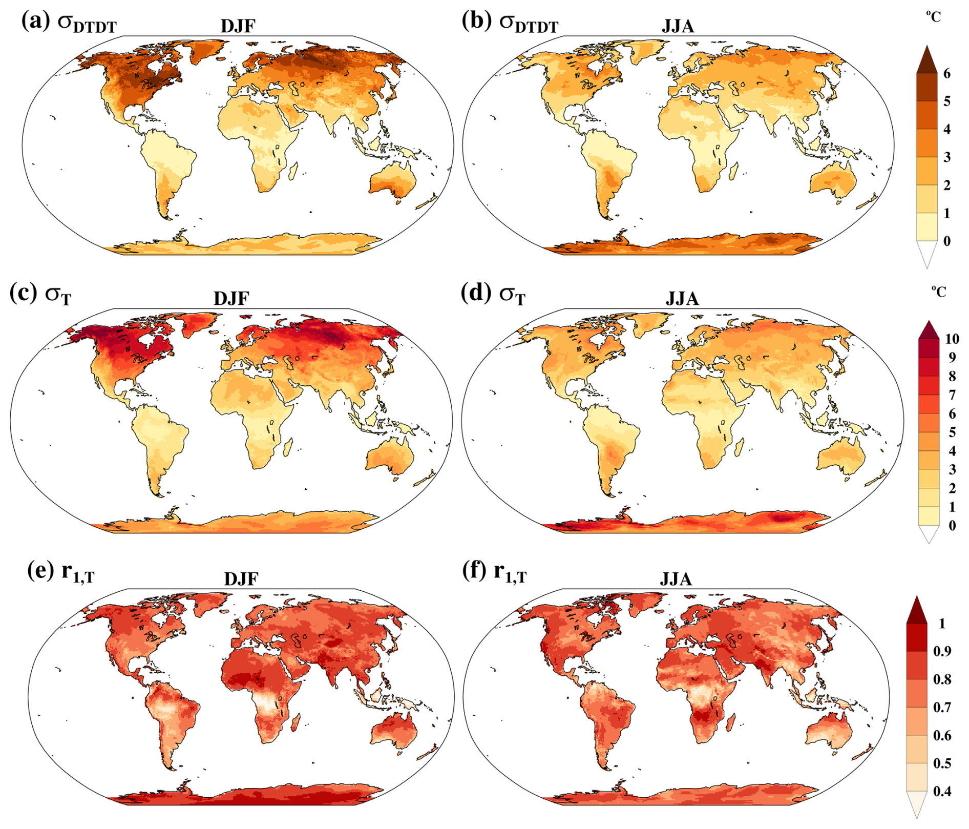
Figure 1 (a, b) The standard deviation of DTDT variations (σ_DTDT, °C), (c, d) the standard deviation of daily mean temperature (σ_T, °C), and (e, f) the lag-1 autocorrelation of daily mean temperature (r_1,T) in December–February (DJF; first column) and June–August (JJA; second column) as derived from the ERA5 dataset.

In HadGHCND, the autocorrelation is spatially rather homogeneous, while there are more pronounced spatial variations with generally lower correlations in the BEST and ERA5 datasets (Figs. 1e–f and S1i–l). Autocorrelation values are typically below 0.8 (and locally below 0.6) in the deep tropics, eastern North America, the Southern Hemisphere land regions south of approximately 30° S, and the eastern half of the Asian continent in JJA, and they are above 0.8 in other regions.

Comparing the global patterns of σ_DTDT, σ_T, and r_1,T shows that the spatial variation in σ_DTDT is mostly determined by variations in σ_T. A high standard deviation σ_T is typically associated with large σ_DTDT in higher latitudes despite the relatively high r_1,T (see again Eq. 5). At the same time, in the tropics, σ_DTDT is smaller because the standard deviation of daily temperature σ_T is low, even though r_1,T is also lower. Nevertheless, r_1,T can affect the spatial pattern of σ_DTDT regionally. For instance, the north–south gradient of r_1,T over Australia in JJA leads to larger σ_DTDT in the south despite relatively homogeneous σ_T. With regard to the differences between observations and ERA5, both a higher σ_T and lower r_1,T in ERA5 contribute to the typically larger σ_DTDT in the reanalysis data.

To gain detailed insights into the statistical distributions of DTDT changes, Fig. S2 shows such distributions for selected locations around the globe – North America, Europe, South America, and Australia. In DJF, North America exhibits the highest variability in DTDT changes, with a broad distribution, whereas South America shows the lowest variability, with a more pronounced peak (Fig. S2a). Europe and Australia experience moderate variability and intermediate kurtosis values, and there is a slight asymmetry (skewness) in the distribution for Australia. In JJA, South America becomes more variable, while North America, Europe, and Australia experience lower variability than in DJF (Fig. S2b), consistent with the seasonal differences in σ_DTDT discussed above. Additionally, the distributions become more negatively skewed in JJA.

3.2 Extreme DTDT changes

To investigate extreme DTDT changes, we use the 5th and 95th percentiles as thresholds at each grid, as illustrated in Fig. 2a–d. The spatial patterns of extreme DTDT changes for both warming and cooling closely resemble those of σ_DTDT and σ_T, with higher values in the extratropics and lower values in the tropics (Fig. 1). This similarity suggests that regions with greater DTDT variations are more prone to extreme DTDT changes. Furthermore, extreme DTDT events are more intense (i.e., exhibit a larger magnitude) during DJF than in JJA, particularly in the Northern Hemisphere. In contrast, the tropics display almost equal magnitudes of extreme DTDT changes in both seasons.

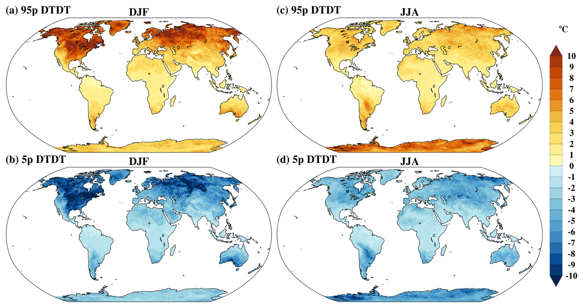
Figure 2 The (a, c) 95th percentile (95p) and (b, d) 5th percentile (5p) of DTDT changes during December–February (DJF; first column) and July–August (JJA; second column) as derived from the ERA5 dataset.

Furthermore, to investigate how DTDT changes relate to the daily temperature of the consecutive days involved, we analyze the relationship between DTDT changes and specific quantiles (terciles) of T_t and T_t−1, as shown in Fig. 3 for North America. Note that similar patterns are observed across other grid boxes (not shown). Our analysis reveals that extreme warming events typically originate in the lower to middle quantiles of T_t−1 and shift toward the middle to higher quantiles of T_t. Conversely, extreme cooling events emerge from the middle to higher quantiles of T_t−1 and transition to the middle to lower quantiles of T_t. The daily temperatures involved in extreme DTDT changes are thus not necessarily extreme but still tend to cluster in the lower/upper tails of the daily temperature distributions. The following section examines the atmospheric circulation patterns and physical processes (as described in Eq. 6) associated with extreme DTDT events at the selected global locations.

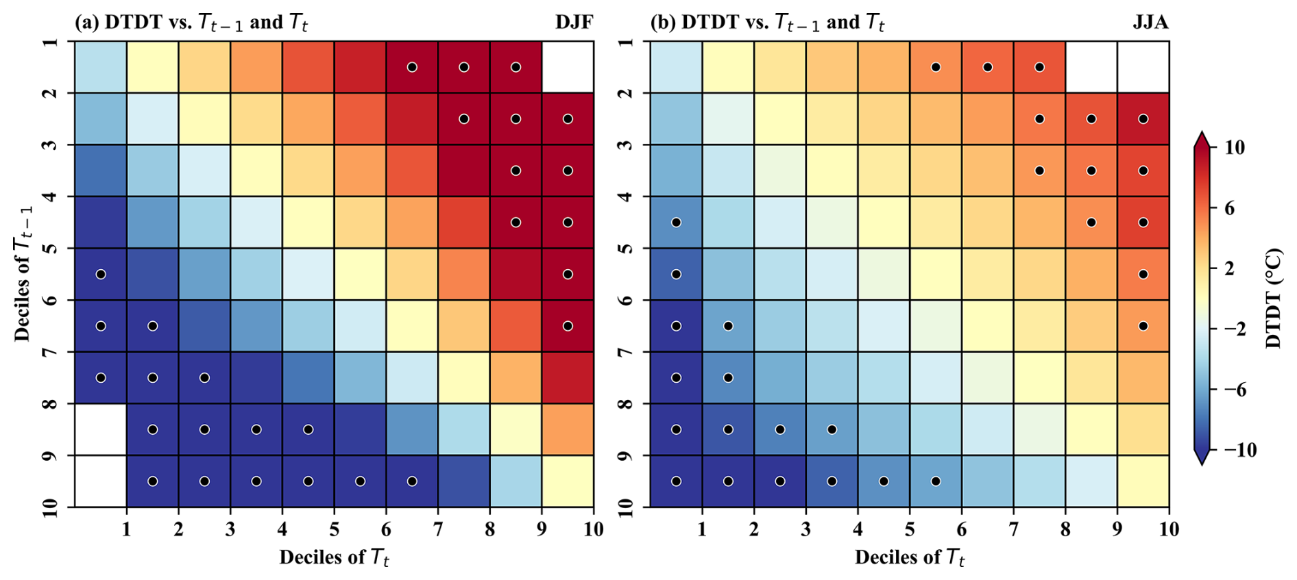
Figure 3 Heatmaps of the relationship between DTDT change and the deciles of temperature on the previous day (T_t−1) and the event day (T_t) for (a) December–February (DJF) and (b) June–August (JJA) for North America. The x axis and y axis represent deciles of T_t and T_t−1, while the color shading indicates DTDT changes, with red and blue colors indicating warming and cooling, respectively. The black circles represent extreme DTDT changes.

3.2.1 Midlatitudes: North America

To explore the mechanism behind extreme DTDT changes in the midlatitudes, we focus on a specific grid box in North America, which is also representative of other North American regions (compare results with Fig. S5).

The synoptic-scale circulation patterns associated with DJF warming events (exceeding the 95th percentile of DTDT changes) on consecutive days and their differences are first analyzed using composites, as shown in Fig. 4a–f. On the day preceding the events (t−1), a near-surface temperature dipole is observed across northern North America, with higher temperatures in the west ($\ge -\mathrm{10}$ °C) and lower temperatures ($\le -\mathrm{15}$ °C) in the east and in the vicinity of the selected location (Fig. 4a). This temperature pattern is influenced by a ridge over the western part, which facilitates southerly winds around its western flank, and a trough over the eastern part of the continent associated with northerly winds (Fig. S3a). This synoptic pattern aligns with the distribution of backward trajectories, indicating the advection of cold air masses from the Arctic region (Fig. 5a). Over the 3 d leading up to this preceding day, these cold air masses (mean temperature of −21.5 °C at −3 d) experience a gradual temperature increase (of 5.7 °C), with significant adiabatic warming (a mean of 8.3 °C) due to a strong 100 hPa mean descent (Fig. 5e–f). Some diabatic cooling, likely due to longwave radiation, is indicated by a reduction in θ (by a mean of −2.6 °C), constraining the temperature increase (Fig. 5g). Accordingly, the temperature at t−1 is mainly determined by the advection of cold, Arctic air masses, whose temperature increases due to adiabatic warming that overcompensates for a slight diabatic cooling.

On the days of the DJF warming events (t), the near-surface temperature reaches $\ge -\mathrm{10}$ °C on average, marking a notable increase compared to at t−1 (Fig. 4b–c). This rise is attributed to an eastward extension of the ridge, displacing the preceding trough further to the east, which leads to southwesterly wind anomalies at the selected location (Fig. S3b). The air parcel density shifts substantially southward compared to at t−1, with the largest density southwest of the chosen location (40–50° N, Fig. 5b). This shift is associated with a substantially higher temperature 3 d before arrival (a mean of −13.4 °C) compared to the air parcels at t−1. The air parcels experience a vertical descent of a mean of 76 hPa (Fig. 5e), leading to adiabatic warming (6.7 °C) and a general temperature increase in the 3 d leading up to the events (Fig. 5f). The net diabatic heating contribution is close to zero (0.4 °C over 3 d) but becomes more prominent in the last hours before the events, reaching 1.2 °C in 24 h (Fig. 5g). Similar to at t−1, the initially colder air masses are thus warmed on their way to the target location. Evaluating the differences in the physical processes between the 2 successive days (Eq. 6) reveals that the changes in advection associated with the shift in the air mass origin and initial temperature are the leading cause for the local DTDT warming at the selected location, contributing 8.1 °C on average (Fig. 5k). Reduced adiabatic warming (−1.6 °C) due to a less pronounced descent on the day of the events counteracts the overall temperature increase, while reduced diabatic cooling (3 °C) provides another positive contribution. This diabatic contribution is associated with the largest event-to-event variation (boxes and whiskers in Fig. 5k).

Warming events in JJA resemble those in DJF, including their atmospheric circulation patterns (not shown) and air parcel density distributions (Fig. S4a–b). The air parcels also experience similar adiabatic warming before arriving at the target location, as in DJF, whereas the diabatic changes have a larger daily cycle and a stronger positive contribution on the last day (Fig. S4e–g). The DTDT warming, as in DJF, is mainly due to the change in the air parcels' initial temperature (0.9 °C at t−1 and 6.4 °C at t) and thus to changes in advection (Fig. S4k). Mean contributions from adiabatic warming and diabatic heating are smaller in magnitude and flip signs compared to in DJF.

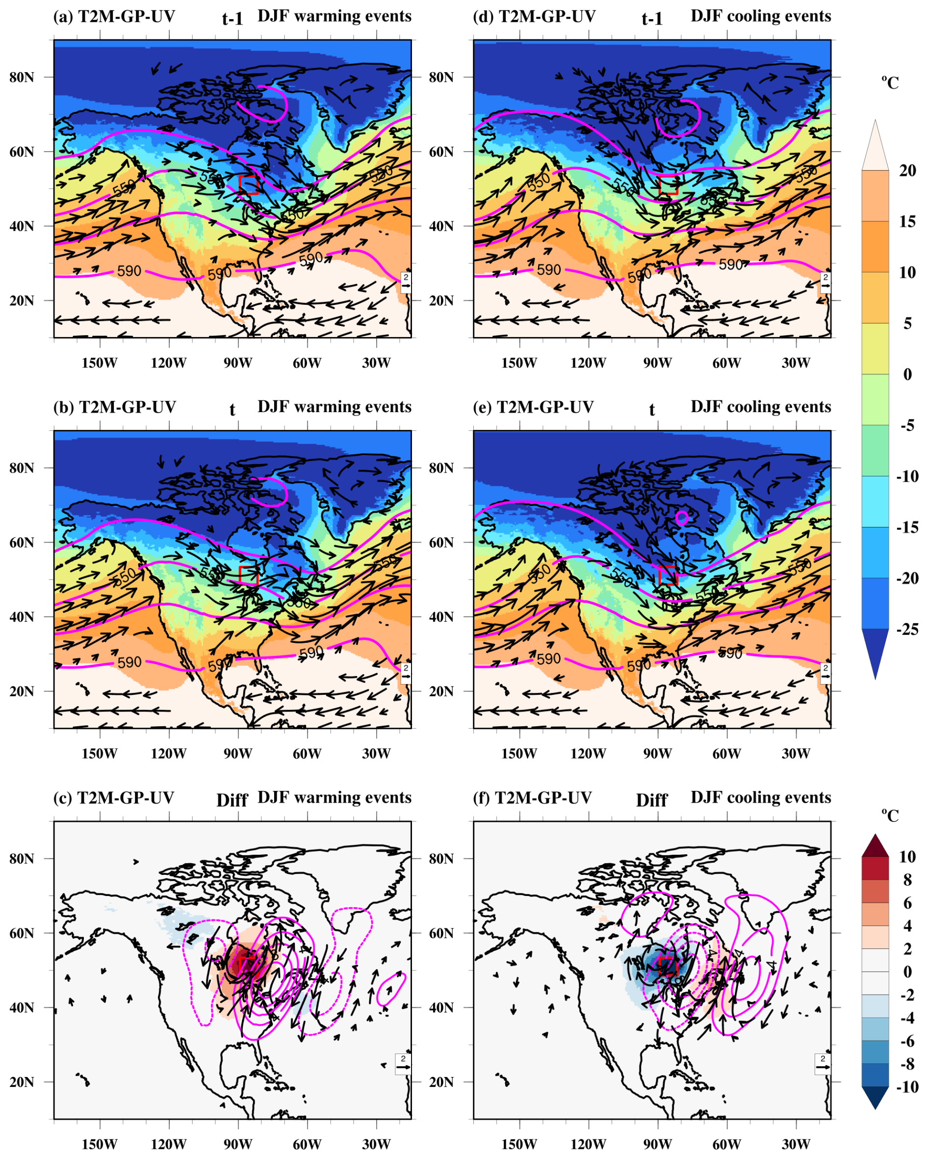
Figure 4 Composite of near-surface temperature (T2M; °C, color shading), wind at 850 hPa (UV; m s⁻¹, vectors), and geopotential height at 500 hPa (GP; gpm, magenta contours) on (a, d) the previous day (t−1) and (b, e) the event day (t) and (c, f) the difference (diff) between the event day and the previous day of the warming (a–c) and cooling (d–f) events during December–February (DJF) at a selected grid box in North America (red box). Note that in panels (a–b and d–e) wind vectors ≥5 m s⁻¹ and in panels (c, f) wind anomalies ≥1 m s⁻¹ are plotted. The dotted and bold magenta contours in (c) and (f) indicate negative and positive geopotential height differences, respectively.

On the days preceding DJF cooling events (t−1), there is a pronounced meridional temperature gradient in the region of the selected location, with near-surface temperature over the northern Arctic land region below −15 °C, while milder temperatures ($\ge -\mathrm{10}$ °C) prevail at the grid box and to its south (Fig. 4d). This thermal gradient is linked to a trough over the Arctic juxtaposed with a ridge structure to its west. Southwesterly winds facilitate the transport of relatively warm air masses towards the location (Figs. S3c and 5c). The transported air parcels, with a mean temperature of −15 °C (at −3 d), undergo a gradual descent, experiencing a modest temperature increase of about 3.7 °C in 3 d that is attributed to the combined effects of adiabatic warming (2.4 °C) and diabatic heating (1.3 °C), as shown in Fig. 5h–j. While the descent and adiabatic warming dominate between −3 and −2 d, the last day before arrival is characterized by diabatic heating (θ increase by 2 °C, Fig. 5j).

On the day of the events (t), a southward shift in the Arctic trough is associated with a turn of the wind towards the north-northwest at the selected location (Figs. 4e and S3d). This corresponds to the arrival of northerly air parcels with an initially extremely low mean temperature of −26.2 °C (Fig. 5d). These air parcels undergo a subsequent temperature increase of 3.2 °C in 3 d due to adiabatic warming (4.3 °C) partly offset by radiative cooling (−1.1 °C, Fig. 5h–j). Accordingly, a shift to strong northerly cold advection (Figs. 4f and 5d) associated with a mean temperature difference of −11.2 °C between the air parcels at −3 d is the predominant contributor to the DTDT cooling events (Fig. 5l). This advective effect is counteracted by moderately increased adiabatic warming (1.9 °C) and complemented by amplified diabatic cooling (−2.4 °C), collectively shaping the DTDT change.

In JJA, the DTDT cooling events are driven by very similar processes as the cooling events during DJF are driven by (Fig. S4). A shift from westerly to northerly transport (Fig. S4c–d) leads to a mean temperature drop of −8.6 °C due to cold-air advection (Fig. S4c–d and h–j). Mean changes in adiabatic and diabatic processes are very small between the 2 d, with larger event-to-event variation (Fig. S4l).

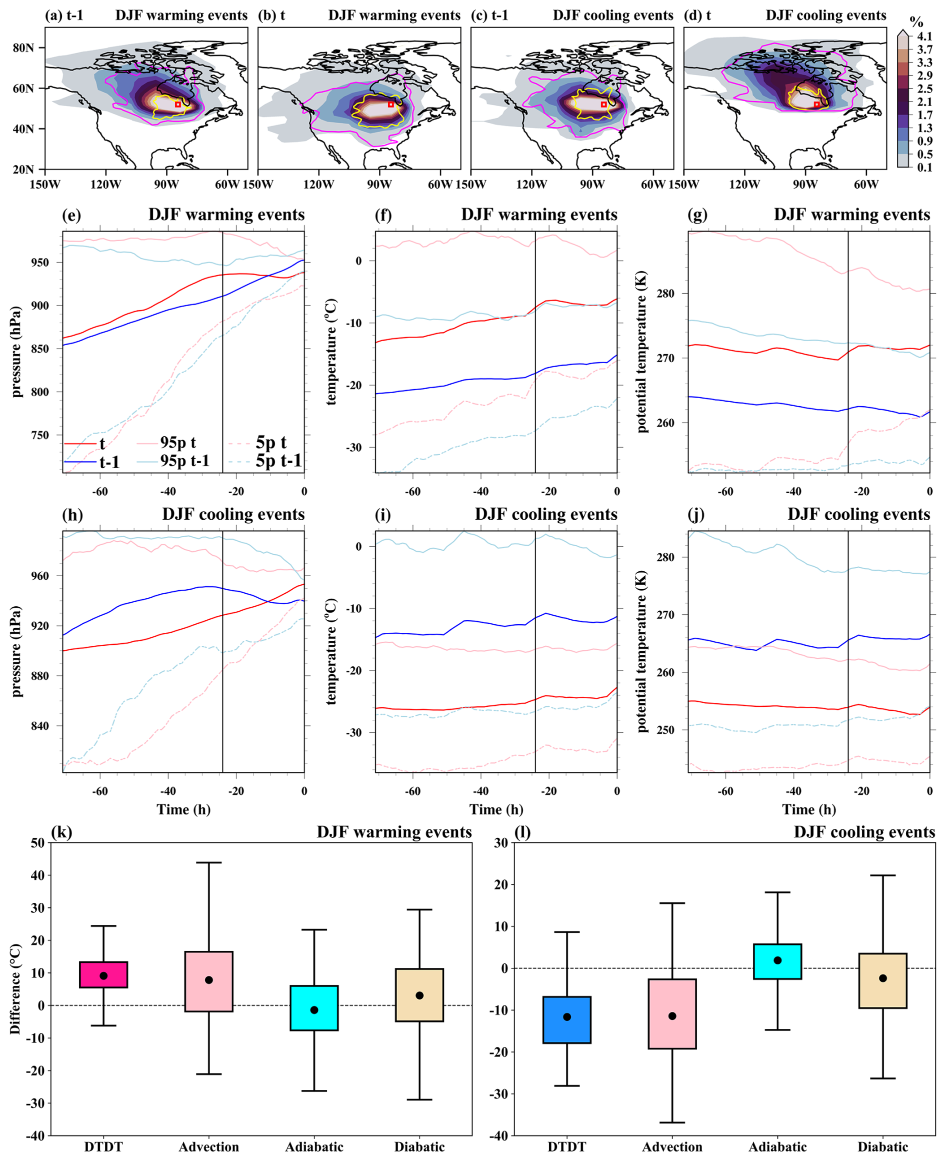
Figure 5 The spatial distribution of trajectories initiated on the previous day (t−1) and on the event day (t) for December–February (DJF) warming and cooling events over North America. In the top row, the color shading illustrates the air parcel trajectory density (%) based on the position between −5 and 0 d. The magenta and yellow contours represent 0.5 % particle density fields at −3 and −1 d, respectively. The red box shows the selected grid box over North America. The Lagrangian evolution of distinct physical parameters (pressure, temperature, potential temperature) along the air parcel trajectories for both warming (second row) and cooling events (third row) is presented in panels (e)–(j). Panels (k) and (l) show the contribution of the different physical processes to the genesis of extreme DTDT changes according to Eq. (6), which refers to a 3 d timescale. The box spans the 25th and 75th percentiles of the data; the black dot inside the box gives the mean of the related quantities; and 1.5 times the interquartile range is indicated by the whiskers.

3.2.2 Midlatitudes: Europe

Another midlatitude location where we investigate the mechanism driving extreme DTDT variations is a grid box over Europe. This section focuses on the JJA season since the DJF events exhibit similarities to the location in North America studied in Sect. 3.2.1.

During the day preceding the JJA warming events (t−1), the composite geopotential height pattern features a weak trough over the eastern North Atlantic and a developing ridge over central Europe (Fig. 6a). In this situation, the northern part of central Europe, including the selected location, is under the influence of westerlies, transporting cool, maritime air masses towards the continent (see Fig. 7a), which are associated with mean temperatures below 18 °C. On the contrary, Spain and western France are already affected by the southwesterly winds associated with the approaching ridge, leading to higher temperatures (≥21 °C) there. The mean initial temperature of the tracked air parcels 3 d before arriving at the selected location is 5.4 °C, and they subsequently undergo a temperature increase of about 10.1 °C in 3 d (Fig. 7f). This increase is partly due to adiabatic warming, corresponding to a mean temperature rise of 5.7 °C, which is linked to a mean pressure increase of 62 hPa. It is worth noting that this subsidence is higher between 3 d and 1 d before arrival and subsequently slows down when the air parcels get close to the surface (Fig. 7e). Diabatic heating, likely to result from surface fluxes, increases the air temperature by 4.4 °C on average, primarily on the last day before arrival.

On the day of the events (t), the trough–ridge pattern typically shifts eastward (Fig. S6b) such that central Europe also is under the influence of the southwesterly wind ahead of the trough (on the western flank of the ridge), and the near-surface temperature rises above 18 °C (Fig. 6b). This warming is associated with the arrival of air masses from western continental Europe (Fig. 7b). These air parcels have a mean initial temperature of 9.3 °C at −3 d, which is substantially warmer than the air masses arriving at t−1, with a subsequent temperature increase of 11.4 °C in 3 d (Fig. 7f). This warming is attributed to adiabatic warming (a mean of 4.5 °C, with a mean descent of 47 hPa) and strong diabatic heating (a mean of 6.9 °C). Comparing the contributions of processes between the 2 d reveals that warm-air advection (3.9 °C, Fig. 7k) is the predominant factor driving the increase in DTDT. Further warming is facilitated by increased diabatic processes (a mean of 2.5 °C). Adiabatic warming, on average, has a small negative contribution (−1.2 °C, the descent is larger at t−1 compared to t), albeit with large variation between events (Fig. 7k).

DJF warming events are dominated by a ridge pattern over western Europe that weakens on the day of the events and is associated with a more zonally oriented flow, bringing a larger fraction of warmer maritime air masses to the selected location, which is in contrast to the mainly continental air parcel origin at t−1 (Figs. S7a–b and S8a–b). This change in origin and the associated warm advection and adiabatic warming are the leading causes of the DTDT increase, whereas diabatic cooling (−5.5 K on both days) does not differ greatly between the 2 d (Fig. S8g and k).

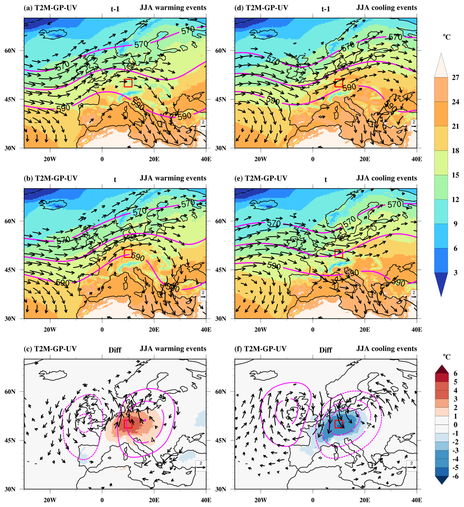
Figure 6 Composite of near-surface temperature (T2M; °C, color shading), wind at 850 hPa (UV; m s⁻¹, vectors), and geopotential height at 500 hPa (GP; gpm, magenta contours) on (a, d) the previous day (t−1) and (b, e) the event day (t) and (c, f) the difference (diff) between the event day and the previous day of the warming (a–c) and cooling (d–f) events during June–August (JJA) at a selected grid box in Europe (red box). Note that in panels (a–b and d–e) wind vectors ≥4 m s⁻¹ and in panels (c, f) wind anomalies ≥1 m s⁻¹ are plotted. The dotted and bold magenta contours in (c) and (f) indicate negative and positive geopotential height differences, respectively.

During the day preceding JJA cooling events (t−1), relatively high near-surface temperatures (≥18 °C) in central Europe are associated with southwesterly winds and warm air masses linked to a trough over the British Isles and a ridge downstream over Scandinavia (Figs. 6d and 7c, S6c). The air parcels are already relatively warm 3 d before they arrive at the selected location (mean temperature of 13.1 °C, Fig. 7i) and are further heated 5.9 °C in 3 d. Adiabatic warming during their descent (3.7 °C, Fig. 7h–i) and diabatic heating (2.2 °C, Fig. 7j) both contribute to this temperature increase.

On the day of the events (t), the central European temperature decreases substantially to values below 18 °C, linked to a weakening of the upstream trough and eastward propagation of the ridge, leading to more zonal flow conditions (Figs. 6e and S6d). Northwesterly winds carry cold, maritime air masses toward the target location, with an initial temperature of 5.4 °C (Fig. 7d and i). These air parcels are further warmed 7.3 °C due to strong adiabatic warming (5.7 °C, corresponding to a mean descent of 60 hPa, Fig. 7h) and some diabatic heating (1.6 °C, Fig. 7j) in 3 d. Comparing the process contributions on the 2 d reveals that DTDT cooling events occur predominantly due to cold-air advection by northerly winds (Fig. 6f), with a mean temperature change of −7.7 °C (Fig. 7l). This advective effect is partly balanced by an increase in adiabatic warming (2 °C). The reduced diabatic heating is small but possesses substantial event-to-event variation (Fig. 7l).

DJF cooling events are triggered by a shift from westerly to northerly winds ahead of a developing ridge over the eastern North Atlantic (Figs. S7e–f and S8c–d). Air masses arriving on the day of the events have a much lower temperature at their origin (−3 d) compared to on the preceding day due to this northward shift in the source location (Fig. S8c–d) and a typically higher altitude (Fig. S8h–j). This leads to a pronounced contribution of advection to the DTDT decrease, which is, however, partly compensated for by increased subsidence and adiabatic warming on the day of the events and by a slight increase in diabatic heating (Fig. S8l).

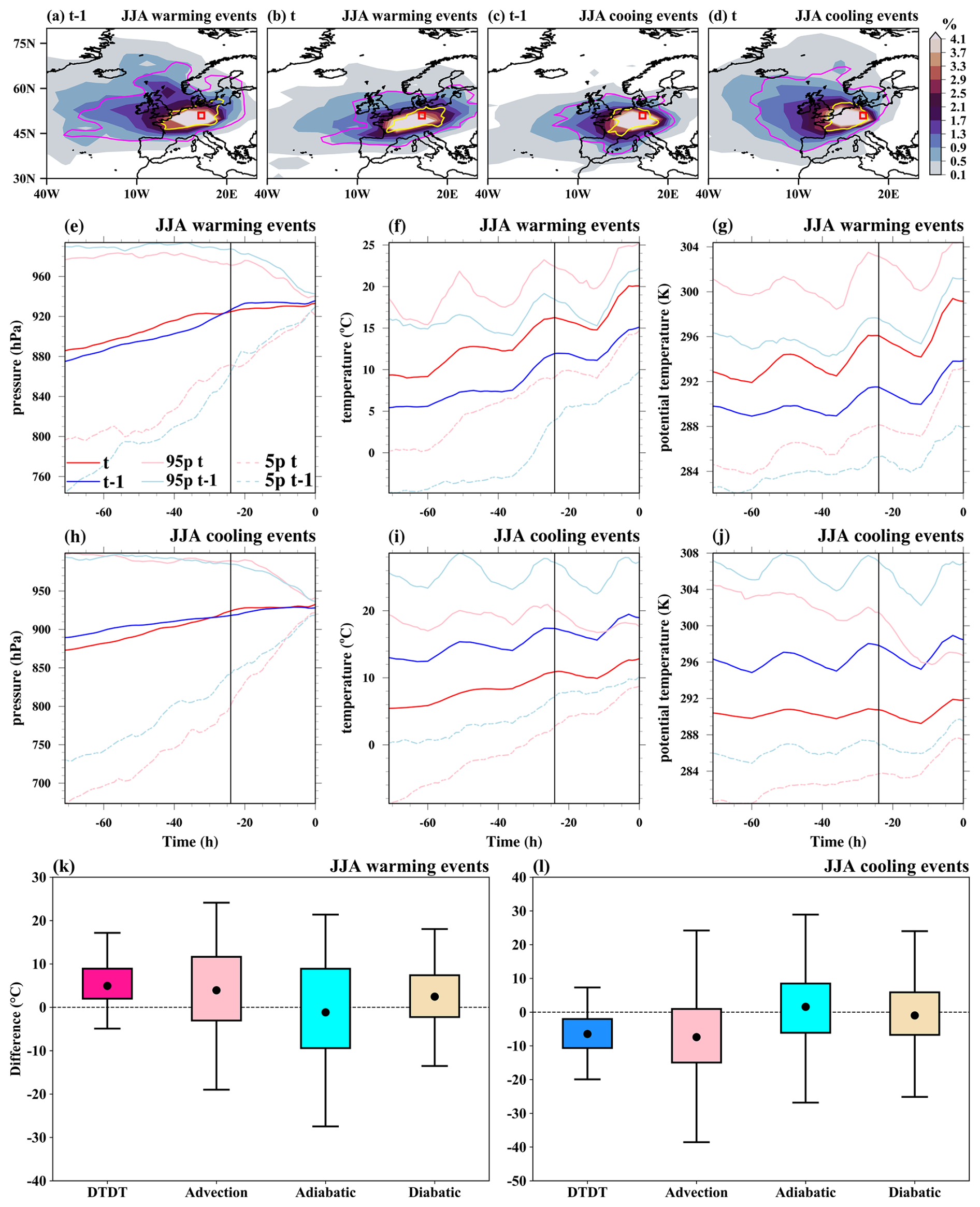
Figure 7 The spatial distribution of trajectories initiated on the previous day (t−1) and the event day (t) for June–August (JJA) warming and cooling events over Europe. In the top row, the color shading illustrates the air parcel trajectory density (%) based on the position between −5 and 0 d. The magenta and yellow contours represent 0.5 % particle density fields at −3 and −1 d, respectively. The red box shows the selected grid box over Europe. The Lagrangian evolution of distinct physical parameters (pressure, temperature, potential temperature) along the air parcel trajectories for both warming (second row) and cooling events (third row) is presented in panels (e)–(j). Panels (k) and (l) show the contribution of the different physical processes to the genesis of extreme DTDT changes according to Eq. (6), which refers to a 3 d timescale. The box spans the 25th and 75th percentiles of the data; the black dot inside the box gives the mean of the related quantities; and 1.5 times the interquartile range is indicated by the whiskers.

3.2.3 Tropics: South America

To investigate the mechanism of extreme DTDT changes in the deep tropics during DJF and JJA, we select a specific location in South America and also compare results with tropical southern Africa (Figs. S10–S11), where physical processes appear to be similar.

During JJA, extreme DTDT changes over tropical South America are associated with distinct patterns, particularly in the wind field (Fig. S9a–f). On the day preceding the warming events (t−1), the selected location lies in the region of a strong horizontal temperature gradient, with higher temperatures (≥22 °C) to the northeast and lower temperatures (≤20 °C) to the southwest. The latter may be associated with extratropical influences, mainly through a trough over Argentina and the South Atlantic (Fig. S9a). Air parcels arriving on this day originate (at −3 d) mainly from the south (Fig. 8a), with a mean initial air temperature of 9.7 °C that gradually increases due to adiabatic warming (4 °C, descent of 41 hPa) and strong diabatic heating (9.9 °C, Fig. 8e–g).

On the day of the warming events (t), the trough weakens, and the winds turn easterly, which is associated with a larger fraction of air parcels originating from the east (Figs. S9b and 8b). These air parcels are initially warmer (12.7 °C on average) than at t−1 (Figs. 8f and S9c) and again experience an average temperature increase (by 13.9 °C) that is influenced by adiabatic warming (5.6 °C, 58 hPa descent) and strong diabatic heating (8.3 °C, Fig. 8e–f). When examining the physical processes across consecutive days, the DTDT warming events can be attributed to a combination of factors, including warm-air advection, enhanced adiabatic warming, and reduced diabatic heating (Fig. 8k). Notably, all three physical factors possess substantial event-to-event variation (Fig. 8l).

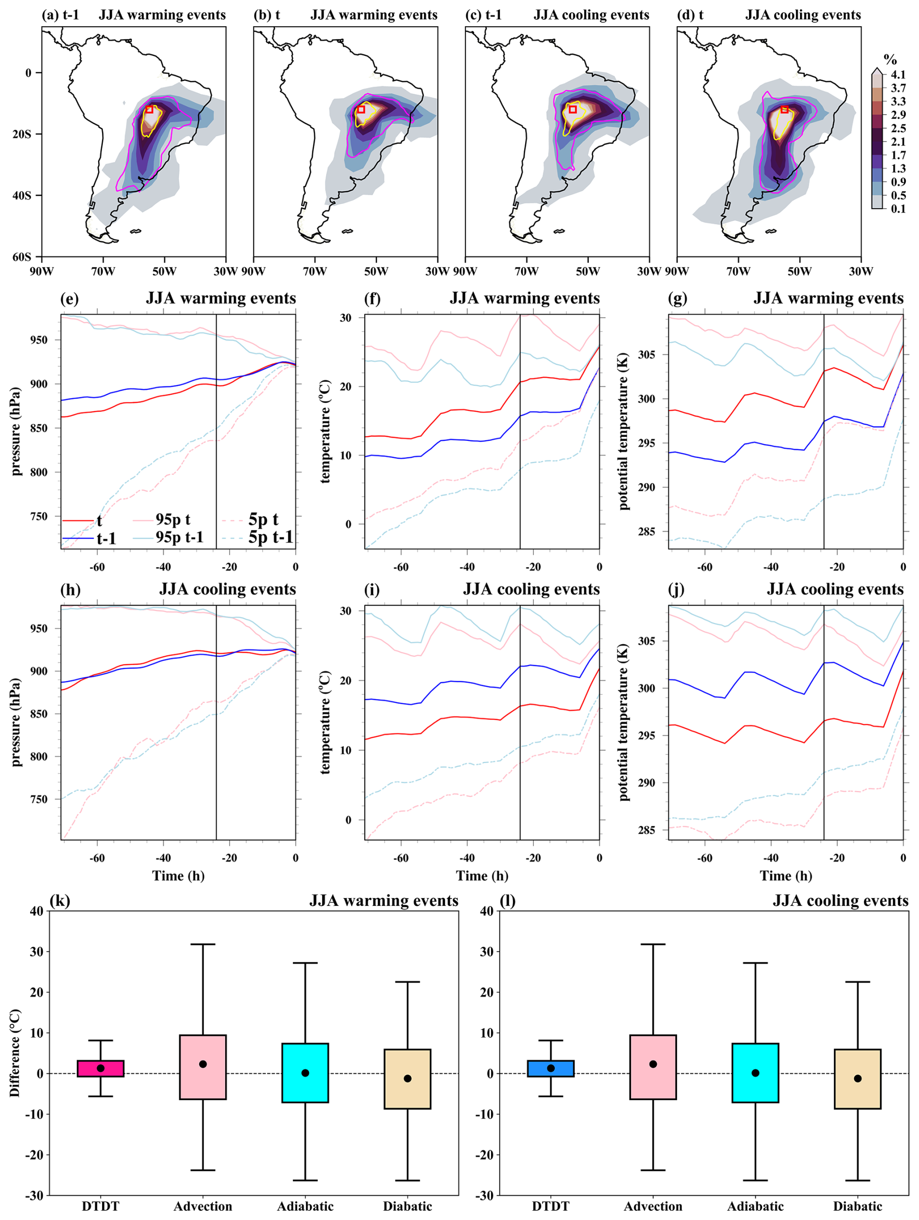
Figure 8 The spatial distribution of trajectories initiated on the previous day (t−1) and on the event day (t) for June–August (JJA) warming and cooling events over South America. In the top row, the color shading illustrates the air parcel trajectory density (%) based on the position between −5 and 0 d. The magenta and yellow contours represent 0.5 % particle density fields at −3 and −1 d, respectively. The red box shows the selected grid box over South America. The Lagrangian evolution of distinct physical parameters (pressure, temperature, potential temperature) along the air parcel trajectories for both warming (second row) and cooling events (third row) is presented in panels (e)–(j). Panels (k) and (l) show the contribution of the different physical processes to the genesis of extreme DTDT changes according to Eq. (6), which refers to a 3 d timescale. The box spans the 25th and 75th percentiles of the data; the black dot inside the box gives the mean of the related quantities; and 1.5 times the interquartile range is indicated by the whiskers.

In contrast to JJA, extreme DTDT changes in DJF are not associated with clear circulation patterns. The origins of air parcels at −3 d are clustered around the selected location, indicating that primarily local effects lead to the DTDT changes (Fig. 9a–d). The advected temperature of air parcels on t and t−1 converge at −24 h (Fig. 9f), and there are only minor changes in descent and adiabatic warming between t and t−1 (Fig. 9e, k). The changes are predominantly due to differences in diabatic heating on the last day before the air parcels arrive at the selected location (Fig. 9e–l). To better understand these local diabatic effects, we analyze composites of cloud cover and precipitation based on ERA5 data (Fig. 10a). For DTDT warming events, high cloud coverage (90 %–95 %), along with substantial cumulative precipitation (10–14 mm d⁻¹), is observed at t−1 across the study region, resulting in reduced diabatic heating and colder temperatures (Figs. 9f–g and 10a). In contrast, cloud cover (70 %–75 %) and precipitation (2–6 mm d⁻¹) decrease on the day of the events, presumably contributing to larger diabatic heating and higher temperatures (Figs. 9f, g, k, and 10b). Thus, the DTDT change during warming events is linked to a transition from primarily cloudy and wet to less cloudy and drier conditions (Fig. 10c). This indicates the essential role of albedo changes and solar radiative heating in triggering the temperature increase.

The day before the JJA cooling events (t−1) is characterized by high near-surface temperatures (≥24 °C) at the selected location and a temperature gradient to the south (Fig. S9d). Easterly winds prevail over the study area, bringing in initially warm air parcels (17.3 °C mean temperature at −3 d) that undergo an additional temperature rise (7.7 °C) due to adiabatic warming (3.3 °C) and diabatic heating (4.4 °C). In contrast, on the day of the events, colder air masses are transported to the selected location by southerly winds upstream and equatorward of a subtropical trough over southeastern South America and the South Atlantic (Figs. 8d and S9e), again pointing to the potential role of extratropical–tropical interactions (Fig. S9f). The air parcels originally have lower temperatures (11.4 °C) than at t−1. They undergo a temperature increase (10.8 °C) due to adiabatic warming (4.4 °C) and diabatic heating (6.4 °C, Fig. 8h–j). Comparing the 2 d indicates that JJA cooling events are driven by cold-air advection, which is partly counterbalanced by increased adiabatic warming and diabatic heating, with larger event-to-event variability (Fig. 8l).

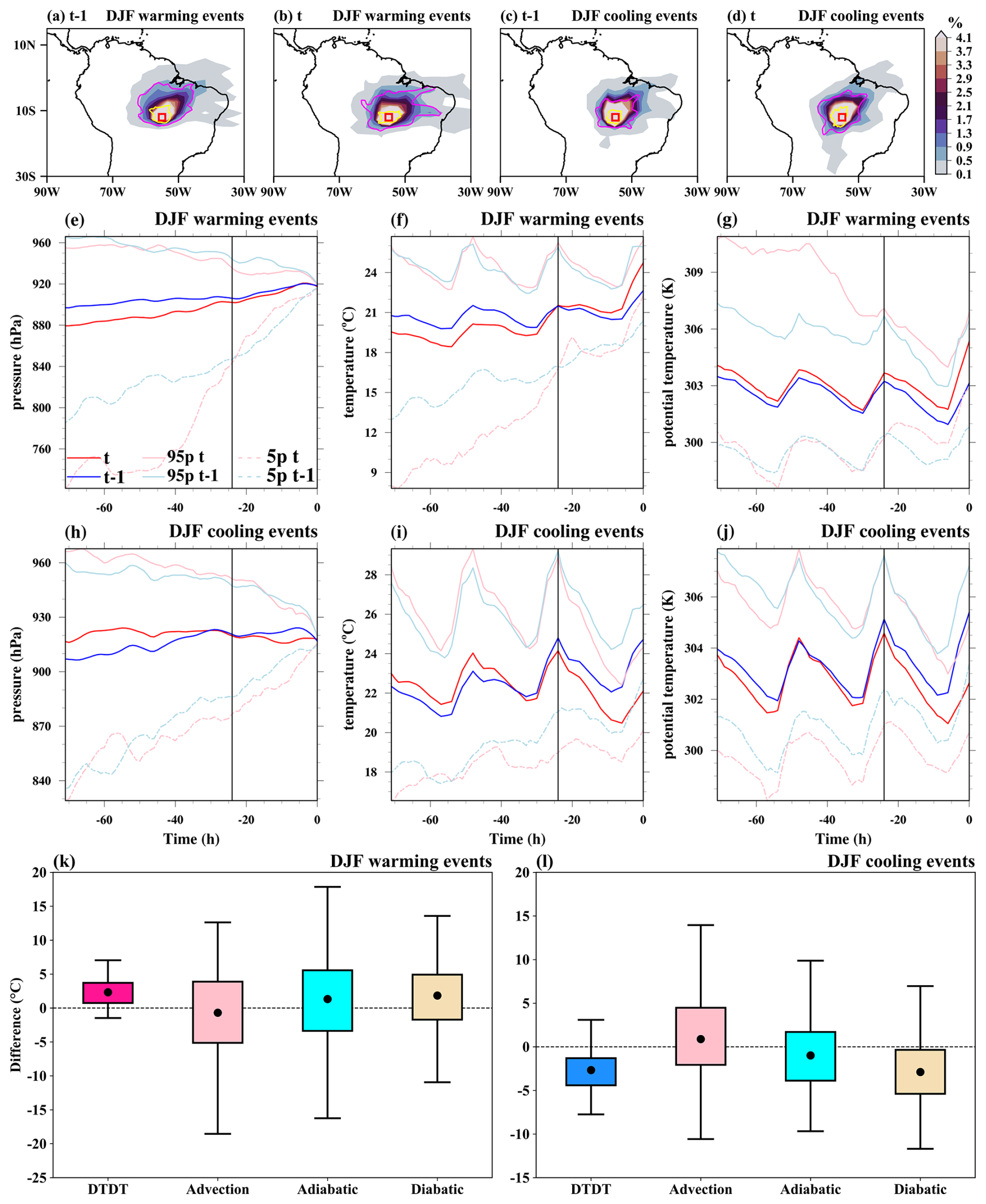
Figure 9 The spatial distribution of trajectories initiated on the previous day (t−1) and on the event day (t) for December–February (DJF) warming and cooling events over South America. In the top row, the color shading illustrates the air parcel trajectory density (%) based on the position between −5 and 0 d. The magenta and yellow contours represent 0.5 % particle density fields at −3 and −1 d, respectively. The red box shows the selected grid box over South America. The Lagrangian evolution of distinct physical parameters (pressure, temperature, potential temperature) along the air parcel trajectories for both warming (second row) and cooling events (third row) is presented in panels (e)–(j). Panels (k) and (l) show the contribution of the different physical processes to the genesis of extreme DTDT changes according to Eq. (6), which refers to a 3 d timescale. The box spans the 25th and 75th percentiles of the data; the black dot inside the box gives the mean of the related quantities; and 1.5 times the interquartile range is indicated by the whiskers.

Similar to the DJF warming events, the DTDT change during DJF cooling events is primarily driven by reduced diabatic heating on the last day before the air parcels arrive at the target location (Fig. 9h–j), which can be attributed to variations in local conditions. Again, like warming events, Fig. 10d–f indicate that these variations are associated with changes in cloud cover and precipitation: on the preceding day, relatively lower cloud cover (70 %–80 %) is observed coupled with lower total precipitation (2–8 mm d⁻¹) across the study area, ultimately resulting in higher temperatures (Figs. 10d and 9i). In contrast, on the day of the events, cloud cover (90 %–95 %) and precipitation (12–20 mm d⁻¹) are higher, contributing to colder temperatures (Figs. 10e and 9i). Thus, DJF cooling events are linked to a transition from less cloudy and drier to cloud-covered and wet conditions (Fig. 10f), again indicating the significant role of solar radiative heating (reduced diabatic heating; see Fig. 9l).

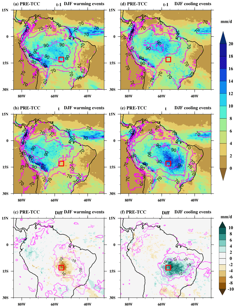
Figure 10 Composites of precipitation (PRE; mm d⁻¹, color shading) and total cloud cover (TCC; %, magenta contours) on (a, d) the previous day (t−1) and (b, e) the event day (t) and (c, f) the difference (diff) between the event day and the previous day of the warming (a–c) and cooling (d–f) events during December–February (DJF) at a selected grid box in South America (red box). The dotted and bold magenta contours in (c) and (f) indicate negative and positive total cloud cover differences, respectively.

3.2.4 Southern Hemisphere subtropics: Australia

We select a specific location in southern Australia to investigate the mechanism driving extreme DTDT changes over the subtropics in the Southern Hemisphere during DJF and JJA.

On the day preceding DJF warming events (t−1), the selected location lies in a region of weak winds in the center of a ridge and within a strong meridional temperature gradient (Fig. S12a), with higher temperatures over the continent to the north (≥24 °C) and lower temperatures over the Southern Ocean (≤16 °C, Fig. 11a). At −3 d, the tracked air parcels are mostly located near the selected box or to its southwest (Fig. 12a). Starting with relatively low temperatures (1.8 °C on average), they undergo substantial subsidence (147 hPa) and adiabatic warming, resulting in a noteworthy temperature increase of 13.8 °C (Fig. 12e–f). In addition, they experience weak diabatic heating on the day before arrival (1.8 °C, Fig. 12g).

The temperature increase on the day of the event is associated with the intensification and eastward shift in a trough towards the Great Australian Bight and the associated northerly winds (Fig. S12b), bringing a warm continental air mass to the selected location (Fig. 11–12b). These air parcels are slightly warmer (5.1 °C) at −3 d compared to at t−1 and also experience adiabatic warming during their descent (9.4 °C, mean descent of 98 hPa) but are much more strongly affected by diabatic heating (9.9 °C, Fig. 12e–g). DJF warming events over the southern coast of Australia thus result from a shift from oceanic to continental air masses (Figs. 11c and S12b), resulting in amplified warm-air advection (3.3 °C) and, more importantly, increased diabatic heating (8.1 °C), most likely due to surface fluxes over the warm continent, while reduced descent and adiabatic warming (−4.4 °C) have a dampening effect, with substantial variability between events (Fig. 12k).

The atmospheric circulation (not shown) and backward air parcel distribution during JJA warming events resemble those of DJF (Fig. S13a–b). However, most probably related to the weaker surface fluxes in austral winter, diabatic heating does not contribute substantially to the temperature evolution along the trajectories (Fig. S13g). Consequently, the warming events are primarily due to warm-air advection (5.9 °C), with both the adiabatic warming (−2.2 °C) and diabatic heating (−1.4 °C) terms having a damping effect (Fig. S13k).

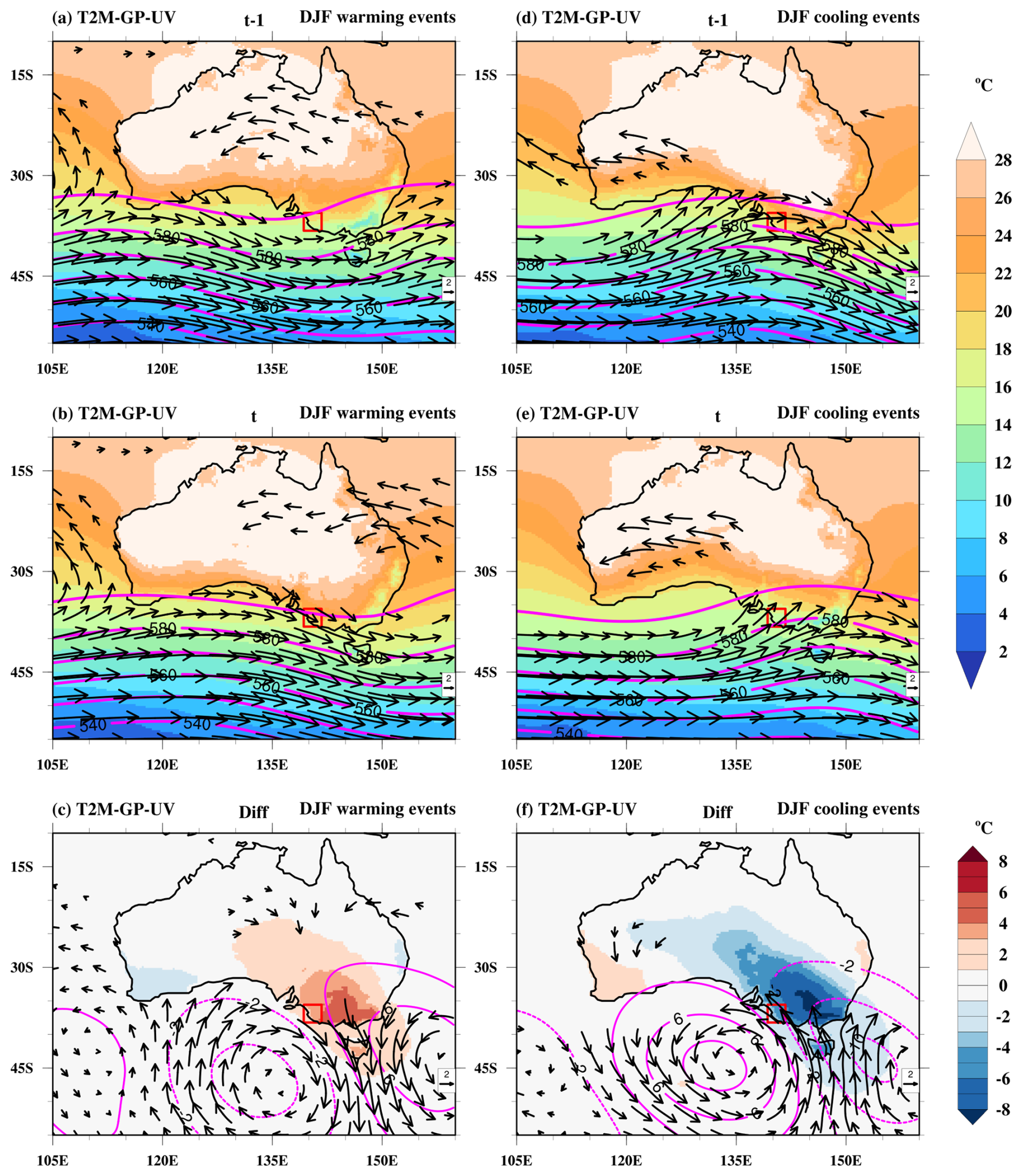
Figure 11 Composite of near-surface temperature (T2M; °C, color shading), wind at 850 hPa (UV; m s⁻¹, vectors), and geopotential height at 500 hPa (GP; gpm, magenta contours) on (a, d) the previous day (t−1) and (b, e) the event day (t) and (c, f) the difference (diff) between the event day and the previous day of the warming (a–c) and cooling (d–f) events during December–February (DJF) at a selected grid box in Australia (red box). Note that in (a–b and d–e) wind vectors ≥4 m s⁻¹ and in (c, f) wind anomalies ≥1 m s⁻¹ are plotted. The dotted and bold magenta contours in (c) and (f) indicate negative and positive geopotential height differences, respectively.

On the day preceding DJF cooling events (t−1), a trough associated with the advection of warm continental air masses is located west of the selected grid box (Figs. 11d, 12c, and S12c). The air particles originate at a relatively high temperature (11.2 °C) and undergo subsequent adiabatic warming (8.5 °C, mean descent of 89 hPa), while diabatic heating is small (Fig. 12h–j). On the day of the events, the trough has moved eastward such that the selected location is under the influence of southwesterly wind on its western side (Figs. 11e–f and S12d), leading to the advection of colder oceanic air masses with a mean temperature of −1.8 °C at −3 d (Fig. 12d–e). This shift to cold-air advection (−13 °C) is the main reason for the DTDT cooling events (Fig. 12l). Adiabatic warming is very similar between the 2 d, while diabatic heating (2.8 °C) increases slightly, dampening the temperature decrease.

Similar to in DJF, JJA cooling events are characterized by a shift from continental to maritime air masses (Fig. 13c–d). The events are mainly triggered by cold-air advection (−10.8 °C) mitigated by increased diabatic heating (6.6 °C), with adiabatic heating (1.3 °C) changes being of minor importance (Fig. S13h–i and l).

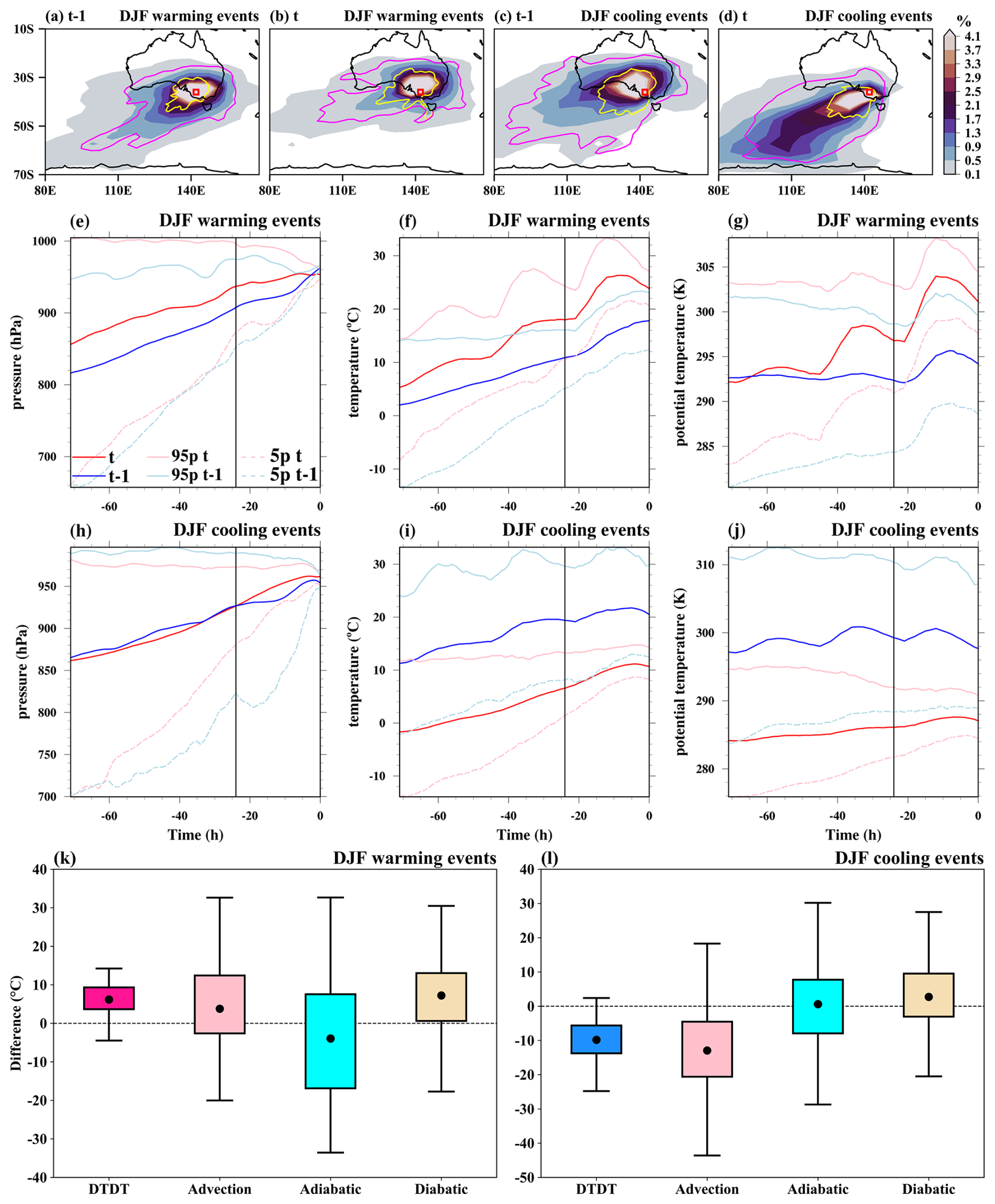
Figure 12 The spatial distribution of trajectories initiated on the previous day (t−1) and on the event day (t) for December–February (DJF) warming and cooling events over Australia. In the top row, the color shading illustrates the air parcel trajectory density (%) based on the position between −5 and 0 d. The magenta and yellow contours represent 0.5 % particle density fields at −3 and −1 d, respectively. The red box shows the selected grid box over Australia. The Lagrangian evolution of distinct physical parameters (pressure, temperature, potential temperature) along the air parcel trajectories for both warming (second row) and cooling events (third row) is presented in panels (e)–(j). Panels (k) and (l) show the contribution of the different physical processes to the genesis of extreme DTDT changes according to Eq. (6), which refers to a 3 d timescale. The box spans the 25th and 75th percentiles of the data; the black dot inside the box gives the mean of the related quantities; and 1.5 times the interquartile range is indicated by the whiskers.

4 Discussion and summary

In this study, we have investigated (extreme) DTDT changes and the underlying physical processes. DTDT changes and extremes have a larger magnitude in the extratropics compared to in tropical regions during both DJF and JJA, consistent with previous studies (Xu et al., 2020; Zhou et al., 2020). These spatial patterns are associated mainly with differences in the standard deviation of daily temperature, but differences in the temporal autocorrelation also play a role in some regional variations. The patterns are generally comparable between ERA5 reanalysis data and observations (particularly BEST), with typically larger magnitudes of DTDT changes in ERA5 (mostly compared to HadGHCND) due to both higher standard deviations and lower autocorrelation. The temperatures on the 2 d associated with extreme DTDT changes are not necessarily extreme by themselves but tend to cluster in the tails of the daily temperature distribution.

The mechanisms driving extreme DTDT changes (cooling events below the 5th percentile and warming events above the 95th percentile) have been analyzed in detail for selected locations using a combination of Eulerian composites and Lagrangian process analysis to decompose the effects of advection and adiabatic and diabatic heating/cooling on a 3 d timescale. In the extratropics, extreme DTDT changes are typically associated with distinct synoptic circulation patterns, in particular troughs and ridges in the 500 hPa geopotential height field, similar to extremes of near-surface temperature (White et al., 2023; Parker et al., 2013; Nygård et al., 2023; see also Fig. S7 for a comparison). These patterns may be related to specific large-scale modes, such as the North Atlantic Oscillation, Arctic Oscillation, or Southern Annular Mode, which significantly impact air mass advection (Lee et al., 2020; Liu et al., 2023; Dai and Deng, 2021). In addition, they are likely associated with frontal passages, as explicitly shown for Europe by Piskala and Huth (2020). Future research may study such potential linkages in more detail, also at other locations.

Our trajectory analysis shows that changes in advection are the main driver of extreme DTDT changes in the extratropics, while the contributions of adiabatic and diabatic processes are generally smaller and vary more in space and also between warming and cooling events. Changes in descent and adiabatic warming between the 2 d of an extreme DTDT change either are small or dampen the intensity of the events, for instance, for warming and cooling events in Europe and southern Asia (Fig. S15c–d) in JJA and in eastern and western North America and southern Asia in DJF (Figs. S5a–b and S15a–b), with the exception of warming events in eastern North America and in high-latitude northern Asia (Fig. S14c–d) in JJA and Europe in DJF, where they contribute positively. Diabatic heating has a particularly strong effect on extreme DTDT changes in southern Australia, where it dampens the events' intensity in JJA but strongly amplifies warming events in the austral summer. The latter is reminiscent of the diabatic effects on wildfires and heat waves in this region (Quinting and Reeder, 2017; Magaritz-Ronen and Raveh-Rubin, 2023). Apart from this, diabatic processes slightly amplify both warm and cold extremes in eastern North America, northern Asia (Fig. S14a–b), southern Asia (Fig. S15a–b), and southern South America (Fig. 16a–b) during DJF and primarily amplify warming events in Europe and western North America (Fig. S5c–d) during JJA. Comparing these processes associated with extreme DTDT changes with the mechanisms leading to the usual temperature extremes (heat and cold waves) indicates similarities in the winter season when temperature extremes are also strongly affected by advection in many midlatitude regions (Bieli et al., 2015; Nygård et al., 2023; Röthlisberger and Papritz, 2023b; Kautz et al., 2022) but shows larger differences in summer, when extreme DTDT events are still primarily driven by advection, whereas advection is, according to several studies, thought to play a smaller role, in particular for temperature extremes and heat waves in larger parts of the midlatitudes (Zschenderlein et al., 2019; White et al., 2023; Röthlisberger and Papritz, 2023a).

We have studied the mechanisms associated with extreme DTDT changes in the tropics for two particular locations at 13° S in South America and tropical southern Africa (see Figs. S10–11) and found large differences between seasons. On the one hand, in JJA, advection is the main contributor to extreme DTDT changes, and interactions with the extratropics play a role, e.g., for the inflow of colder air masses towards lower latitudes during cooling events upstream of a subtropical trough. This configuration resembles the circulation impacting the cold waves in central South America (Marengo et al., 2023) and tropical southern Africa (Chikoore et al., 2024) in JJA 2021. On the other hand, during DJF, extreme DTDT changes occur primarily due to local-scale diabatic processes associated with changes from cloudy conditions with precipitation to less cloudy and drier conditions or vice versa. This points to the important role of cloud radiative effects in these events, primarily through the reflection of solar radiation (see Dai et al., 1999; Betts et al., 2013; Medvigy and Beaulieu, 2012).

Our study provides the first quantitative insights into the physical atmospheric processes that lead to extreme temperature changes from one day to another. The role of changing advection from warmer or colder regions in extreme DTDT changes is apparent across all studied regions except the tropics during DJF. Such advective effects are modified by Lagrangian temperature changes due to adiabatic or diabatic processes, which tend to either amplify or dampen extremely positive (warming events) and negative (cooling events) DTDT changes, depending on the region and season. This dominant effect of advection also explains why the magnitude of DTDT changes is typically larger in the extratropics, where horizontal temperature gradients and wind velocities are larger compared to in the tropics. The magnitude of the adiabatic and diabatic terms in our Lagrangian budgets is of the same magnitude in the extratropics and tropics and thus cannot compensate for this difference in advection. These mechanistic insights will be the basis for studying projected future changes in extreme DTDT changes in the second part of this study.

Appendix A

The DTDT (δ_T) change defined in Eq. (1), which has been determined based on the temperature 2 m above the surface, is approximated through the average temperatures of the trajectories initiated on the corresponding day at their initiation time 0, denoted ${\mathit{\delta }}_T^{\mathrm{0}}$:

$$\begin{array}{}\text{(A1)}& {\mathit{\delta }}_T\approx {\mathit{\delta }}_T^{\mathrm{0}}={\stackrel{\mathrm{‾}}{T}}_t^{\mathrm{0}}-{\stackrel{\mathrm{‾}}{T}}_{t-\mathrm{1}}^{\mathrm{0}}.\end{array}$$

Note that the lower index here refers to the day on which the trajectories were initiated, and the upper index refers to the time along the backward trajectory. This equation contains an approximation, as the trajectories are initialized only once a day (while δ_T refers to daily average temperatures) and from different heights above the surface, assuming (and sampling) a well-mixed near-surface layer. These trajectory temperatures can then be expressed through the Lagrangian temperature evolution:

$$\begin{array}{}\text{(A2)}& \begin{array}{rl}{\mathit{\delta }}_T^{\mathrm{0}}& ={\stackrel{\mathrm{‾}}{T}}_t^{\mathrm{0}}-{\stackrel{\mathrm{‾}}{T}}_{t-\mathrm{1}}^{\mathrm{0}}\\ & ={\stackrel{\mathrm{‾}}{T}}_{\mathrm{t}}^{\mathrm{0}}-{\stackrel{\mathrm{‾}}{T}}_{\mathrm{t}}^{-\mathrm{3}\mathrm{d}}-{\stackrel{\mathrm{‾}}{T}}_{t-\mathrm{1}}^{\mathrm{0}}+{\stackrel{\mathrm{‾}}{T}}_{t-\mathrm{1}}^{-\mathrm{3}\mathrm{d}}+{\stackrel{\mathrm{‾}}{T}}_t^{-\mathrm{3}\mathrm{d}}-{\stackrel{\mathrm{‾}}{T}}_{t-\mathrm{1}}^{-\mathrm{3}\mathrm{d}}\\ & ={\mathrm{\Delta }}_{\stackrel{\mathrm{‾}}{T},t}-{\mathrm{\Delta }}_{\stackrel{\mathrm{‾}}{T},t-\mathrm{1}}+{\mathit{\delta }}_{\stackrel{\mathrm{‾}}{T}}^{-\mathrm{3}\mathrm{d}}.\end{array}\end{array}$$

Here, ${\mathrm{\Delta }}_{\stackrel{\mathrm{‾}}{T},t-\mathrm{1}}={\stackrel{\mathrm{‾}}{T}}_{t-\mathrm{1}}^{\mathrm{0}}-{\stackrel{\mathrm{‾}}{T}}_{t-\mathrm{1}}^{-\mathrm{3}\mathrm{d}}$ and ${\mathrm{\Delta }}_{\stackrel{\mathrm{‾}}{T},t}={\stackrel{\mathrm{‾}}{T}}_t^{\mathrm{0}}-{\stackrel{\mathrm{‾}}{T}}_t^{-\mathrm{3}\mathrm{d}}$ denote the Lagrangian temperature change along the trajectories on a 3 d timescale for the previous day and the day of the event. The term ${\mathit{\delta }}_T^{-\mathrm{3}\mathrm{d}}={\stackrel{\mathrm{‾}}{T}}_t^{-\mathrm{3}\mathrm{d}}-{\stackrel{\mathrm{‾}}{T}}_{t-\mathrm{1}}^{-\mathrm{3}\mathrm{d}}$ is used to measure the contribution due to advection.

This advection term differs from that of Röthlisberger and Papritz (2023b, a), who focused on daily temperature extremes and used horizontal advection of the air parcel along the climatological temperature gradient as a measure of advection in their temperature anomaly budget. This is not possible here since our diagnostic is based on absolute temperatures and not on anomalies. Technically, ${\stackrel{\mathrm{‾}}{T}}_t^{-\mathrm{3}\mathrm{d}}$ represents the average temperature of the air parcels initialized on the day of the extreme event, 3 d before they arrive at the target location, while ${\stackrel{\mathrm{‾}}{T}}_{t-\mathrm{1}}^{-\mathrm{3}\mathrm{d}}$ represents the corresponding temperature for the air parcels initialized 1 d earlier. The expression in Eq. (A2), ${\mathit{\delta }}_T^{-\mathrm{3}\mathrm{d}}={\stackrel{\mathrm{‾}}{T}}_t^{-\mathrm{3}\mathrm{d}}-{\stackrel{\mathrm{‾}}{T}}_{t-\mathrm{1}}^{-\mathrm{3}\mathrm{d}}$, thus captures the difference in temperature between the air parcels 3 d before their arrival. Assuming that no further temperature changes occurred during transport, the DTDT change would be solely due to these initial differences. This suggests that variations in the advection of air parcels with different original temperatures between the previous day and the day of the event cause temperature changes, which is referred to as the advection term here.

The Lagrangian temperature change can be further decomposed into the adiabatic and diabatic contributions using the thermodynamic energy equation:

$$\begin{array}{}\text{(A3)}& {\displaystyle \frac{\mathrm{d}T}{\mathrm{d}t}}={\displaystyle \frac{\mathit{\kappa }T\mathit{\omega }}{p}}+{\left({\displaystyle \frac{p}{p_{\mathrm{0}}}}\right)}^{\mathit{\kappa }}{\displaystyle \frac{\mathrm{d}\mathit{\theta }}{\mathrm{d}t}}.\end{array}$$

T is temperature, $\frac{\mathrm{d}T}{\mathrm{d}t}$ is the temperature change along the trajectory, κ=0.286, p denotes pressure (p₀=1000 hPa), ω is the vertical velocity in pressure coordinates, and θ is the potential temperature.

Accordingly,

$$\begin{array}{}\text{(A4)}& {\mathrm{\Delta }}_{\stackrel{\mathrm{‾}}{T},t}=\langle \underset{-\mathrm{3}\mathrm{d}}{\overset{\mathrm{0}}{\int }}{\displaystyle \frac{\mathrm{d}{T}_{t,i}}{\mathrm{d}\mathit{\tau }}}\mathrm{d}\mathit{\tau }{\rangle }_i,\end{array}$$

where T_t,i is the temperature along the ith trajectory, $\langle \mathrm{\dots }{\rangle }_{\mathrm{i}}={\sum }_{i=\mathrm{1}}^m\frac{\mathrm{1}}{m}$ … denotes the average over the m trajectories, and τ is the time along the trajectory. Inserting Eq. (A4) into (A3) yields

$$\begin{array}{}\text{(A5)}& {\mathrm{\Delta }}_{\stackrel{\mathrm{‾}}{T},t}={\mathrm{\Delta }}_{\stackrel{\mathrm{‾}}{T},t}^{\mathrm{adi}}+{\mathrm{\Delta }}_{\stackrel{\mathrm{‾}}{T},t}^{\mathrm{dia}},\end{array}$$

with the adiabatic term $\left({\mathrm{\Delta }}_{\stackrel{\mathrm{‾}}{T},t}^{\mathrm{adi}}\right)=\langle {\int }_{-\mathrm{3}\mathrm{d}}^{\mathrm{0}}\frac{\mathit{\kappa }T\mathit{\omega }}{p}\mathrm{d}\mathit{\tau }{\rangle }_{\mathrm{i}}=\langle {\int }_{p^{-\mathrm{3}\mathrm{d}}}^{p^{\mathrm{0}}}\frac{\mathit{\kappa }T}{p}\mathrm{d}p{\rangle }_i$ and the diabatic term $\left({\mathrm{\Delta }}_{\stackrel{\mathrm{‾}}{T},t}^{\mathrm{dia}}\right)={〈{\int }_{-\mathrm{3}\mathrm{d}}^{\mathrm{0}}{\left(\frac{p}{p_{\mathrm{0}}}\right)}^{\mathit{\kappa }}\frac{\mathrm{d}\mathit{\theta }}{\mathrm{d}\mathit{\tau }}\mathrm{d}\mathit{\tau }〉}_i={〈{\int }_{{\mathit{\theta }}^{-\mathrm{3}\mathrm{d}}}^{{\mathit{\theta }}^{\mathrm{0}}}(\frac{p}{p_{\mathrm{0}}}{)}^{\mathit{\kappa }}\mathrm{d}\mathit{\theta }〉}_i$.

Then Eq. (A2) becomes

$$\begin{array}{}\text{(A6)}& \begin{array}{rl}{\mathit{\delta }}_T^{\mathrm{0}}& ={\mathit{\delta }}_{\stackrel{\mathrm{‾}}{T}}^{-\mathrm{3}\mathrm{d}}+{\mathrm{\Delta }}_{\stackrel{\mathrm{‾}}{T},t}^{\mathrm{adi}}-{\mathrm{\Delta }}_{\stackrel{\mathrm{‾}}{T},t-\mathrm{1}}^{\mathrm{adi}}+{\mathrm{\Delta }}_{\stackrel{\mathrm{‾}}{T},t}^{\mathrm{dia}}-{\mathrm{\Delta }}_{\stackrel{\mathrm{‾}}{T},t-\mathrm{1}}^{\mathrm{dia}}\\ & ={\mathit{\delta }}_{\stackrel{\mathrm{‾}}{T}}^{-\mathrm{3}\mathrm{d}}+{\mathit{\delta }}_{\stackrel{\mathrm{‾}}{T}}^{\mathrm{adi}}+{\mathit{\delta }}_{\stackrel{\mathrm{‾}}{T}}^{\mathrm{dia}}.\end{array}\end{array}$$

In Eq. (A6), ${\mathit{\delta }}_T^{\mathrm{0}}$ is the approximated near-surface DTDT change; ${\mathit{\delta }}_{\stackrel{\mathrm{‾}}{T}}^{-\mathrm{3}\mathrm{d}}$ measures the mean temperature difference at the origin of the air parcels and thus the contribution of advection on a 3 d timescale; ${\mathit{\delta }}_{\stackrel{\mathrm{‾}}{T}}^{\mathrm{adi}}$ is the mean temperature difference created through adiabatic compression or expansion resulting from vertical descent or ascent, respectively; and ${\mathit{\delta }}_{\stackrel{\mathrm{‾}}{T}}^{\mathrm{dia}}$ is the contribution of mean diabatic heating or cooling from processes such as latent heating in clouds, radiation, and surface fluxes.