Glacier thinning causes warmer and drier regional climate at the Jostedalsbreen ice cap in western Norway

Glacier recession gives rise to changes in land surface type and topography that are poorly represented in atmospheric models but may have important local impacts on climate. Implementing these changes in the Weather Research and Forecasting (WRF) model for the Jostedalsbreen ice cap in western Norway results in warmer and drier regional climate with less snow that can amplify glacier recession through a positive feedback effect. Most of the climatic response to glacier recession is related to the surface lowering associated with ice melt, resulting in reduced orographic lifting of moist air masses and higher surface pressure. The climatic response to glacier recession is largest where the ice melts but is also evident in adjacent valleys several kilometers away from the ice cap. While the warming by glacier recession amplifies effects of global warming, reduced precipitation counteracts the projected regional increase in precipitation. These findings should be included in estimates of glacier mass balance and have implications for agriculture, hydropower, tourism, and biodiversity around glacierised landscapes.

1 Introduction

Glaciers worldwide are melting due to global warming, yet our understanding of how receding glaciers influence regional climate remains poor. Glacier recession exposes the underlying landscape, which typically lowers the albedo (Kotlarski et al., 2010; Di Mauro, 2020; Zhang et al., 2021). This results in increased absorption of solar radiation and a positive feedback with accelerated glacier melt and further near-surface warming. Along with changes in glacier extent, glacier recession also lowers the terrain by thinning the ice. This has direct consequences for local weather and climate, as topography affects the role of orographic precipitation, temperature, and topographically forced wind systems. Despite the feedback from changes in albedo and topography on meteorological variables, few studies have investigated their importance in a changing climate.

Mountain glacier retreat has, in some weather conditions, been found to influence local weather by weakening glacier (katabatic) winds and modifying convection patterns and mountain wave activity nearby (Goger et al., 2025; Haualand et al., 2025). Glacier winds, which are forced by strong thermal contrasts over a sloping ice surface, advect cold air from upper to lower parts of a glacier and enhance the entrainment of surrounding air toward the glacier surface through increased turbulent sensible and latent heat fluxes (e.g., van den Broeke, 1997; Oerlemans, 2010). The relative change in cold air advection and warm air entrainment when glacier winds weaken is important for local melt rates and depends on factors such as glacier slope angle, background flow, and atmospheric stability in the glacier boundary layer (Sauter et al., 2026). The ambient warming that leads to glacier recession in a changing climate enhances the atmospheric stability and potentially the sensible heat fluxes above the melting glacier surface. As sensible heat fluxes drive the glacier wind (e.g., Oerlemans, 2010; Sauter and Galos, 2016; Sauter et al., 2026), their potential enhancement in a warmer environment may compensate for some or all of the weakening of the glacier wind directly associated with glacier recession (Salerno et al., 2023). As a result, ambient warming may be accompanied by enhanced advection of cold air masses by glacier winds that causes less warming of the glacier boundary layer compared to its surroundings (Salerno et al., 2023; Shaw et al., 2025). It is, however, still an open question how dominant the response in cold air advection by glacier winds is relative to the increase in warm air entrainment into the glacier boundary layer associated with global warming. The overall balance between these climate-induced local cooling and warming effects of the glacier surface depends on the extent of the glacier and the state of the background climate (Shaw et al., 2024, 2025). It is therefore important to investigate the impact of glacier recession on local climate over large spatial and temporal scales representing a variety of glaciological and meteorological conditions.

The complex terrain that often surrounds mountain glaciers introduces large spatial variations in topographically forced wind systems and precipitation (e.g., Frei and Schär, 1998; Esau and Repina, 2012; Sauter, 2020; Temme et al., 2020; Goger et al., 2025; Sauter et al., 2026). Due to orographic lifting of moist air masses that hit mountains, precipitation is typically concentrated near ridges or on the windward side of the mountain range, with local variations existing due to effects from slope, atmospheric stability, interactions with clouds, and local wind systems (Frei and Schär, 1998; Houze, 2012; Sauter, 2020). In glacial landscapes, Salerno et al. (2023) argue that local precipitation rates depend on the strength of the katabatic wind system, which can shift wind convergence zones and the associated convection away from a glacier if the down-glacier wind is strong enough. There is, however, little research on how changes in glacier extent and elevation affect regional precipitation and atmospheric circulation patterns (Sauter et al., 2026), despite ongoing and projected widespread and rapid recession of glaciers worldwide.

Along with potential impacts on local weather, receding glaciers may form new proglacial lakes in topographic depressions that become ice-free (e.g., Ekblom Johansson et al., 2022; Gillespie et al., 2024a). Changes in extent and temperature of these lakes as well as the distance between the glacier and the lake, can modify the microclimate around the glacier-lake system (Haualand et al., 2025). Still, no studies have, to the authors' knowledge, studied how potential future lakes that form due to glacier recession influence regional climate.

Numerical weather prediction models are a potent tool to study the impact of the aforementioned changes in glacial landscapes on weather and climate. To represent key meteorological processes such as precipitation and snow cover and their spatial and temporal distribution in mountainous areas, high horizontal model resolution at the kilometer scale is needed (Pontoppidan et al., 2017; Lüthi et al., 2019; Ban et al., 2021; Pichelli et al., 2021; Fosser et al., 2024). In this study, we utilize a numerical weather prediction model at 1 km horizontal resolution to analyse multi-year climatic responses to a changing glacier environment in the complex terrain around the Jostedalsbreen ice cap in western Norway. This ice cap is topographically diverse and is therefore representative for many other glacierised areas of the world with a temperate climate. While daily near-surface temperature in complex glacier environments is in general typically well resolved at 1 km resolution (Claremar et al., 2012; Eidhammer et al., 2021; Draeger et al., 2024), it is often challenging to accurately represent temperature inversions and cold air pools due to their shallow scales (Haualand et al., 2025). Partly related to this, many important valleys in our study area, e.g., those where outlet glaciers of the Jostedalsbreen ice cap terminate, are at this resolution only covered by a few grid cells, which is not enough to appropriately resolve local wind systems (Wagner et al., 2014). Nevertheless, cold air pools and katabatic and topographically forced winds were partly resolved by the 1 km model resolution and setup in a recent case study of a representative subdomain of this region (Haualand et al., 2025). This suggests that the most important phenomena for a climatic study like the present one are represented well enough and that running the model with a higher horizontal resolution will be at the expense of simulation time. While higher model resolution can improve the representation of finer scales and their interactions with larger scales, the additional scientific insight will likely remain limited due to the need for more smoothing of the terrain to avoid numerical instability (Pontoppidan et al., 2017). Furthermore, in WRF simulations of three glaciers on Svalbard with kilometer-scale resolution, Claremar et al. (2012) argued that increasing the vertical resolution at lower levels is often more important for the wind speed than increasing the horizontal resolution. With this in mind, we use a compromised setup of WRF, with dense vertical grid spacing near ground, that targets key climatic processes in a long term perspective.

The objectives of this study are to (i) provide the most detailed spatial representation of the recent climate around the Jostedalsbreen ice cap, (ii) determine regional changes in temperature and precipitation associated with future glacier recession and the associated potential formation of new lakes, and (iii) compare climatic changes directly associated with global warming with changes due to ice loss.

2 Study area

Jostedalsbreen, the largest ice cap in mainland Europe, is located in western Norway and is surrounded by complex terrain including fjords, narrow and steep valleys, and mountains up to more than 2000 m a.s.l (Fig. 1). The ice cap covers 458 km² (in 2019; Andreassen et al., 2022), and the thickest ice is more than 600 m thick (Gillespie et al., 2024a). Jostedalsbreen has lost 3 % of its area from 2006 to 2019 (Andreassen et al., 2023) and is projected to lose 49 % of its mass by the end of the century for the emissions pathway RCP4.5 and 63 % for RCP8.5 (Åkesson et al., 2025). Along with glacier recession, new lakes are projected to form in topographic depressions exposed by the shrinking ice cap (Gillespie et al., 2024a). These potential future lakes may cover 14 % of the present-day glacier area if all the ice of Jostedalsbreen is lost.

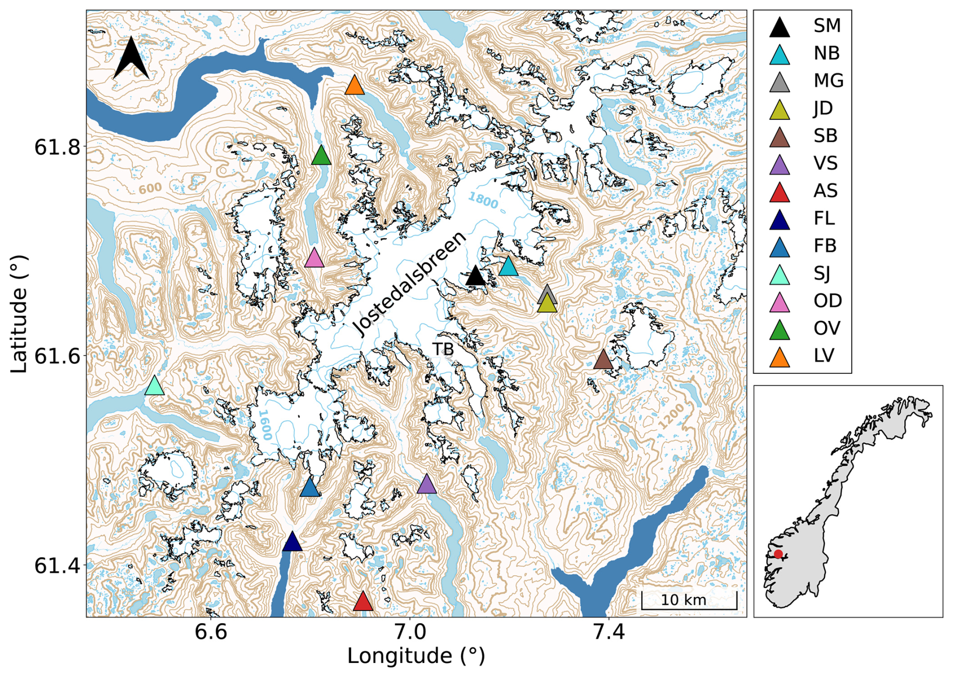
Figure 1 Map of study area including weather stations used for validation (triangles). White, light blue, and dark blue areas represent ice and snow surfaces, inland lakes, and fjords, respectively. Thin (thick) brown and blue contours represent elevation contours from Norwegian Mapping Authorities (2025) every 200 (1000) m over ice-free and ice-covered surfaces, respectively, with some selected contours labelled. “TB” indicates the location of Tunsbergdalsbreen, the largest outlet glacier of the Jostedalsbreen ice cap.

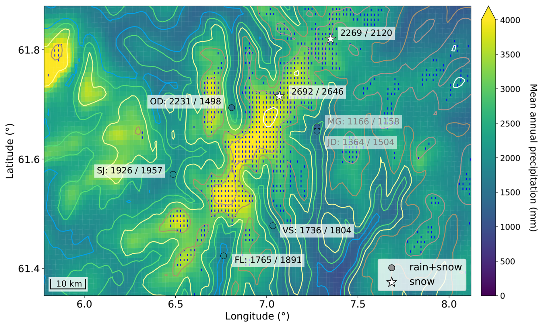
Figure 2 Mean annual precipitation from model (shading) and AWSs (colored dots) and locations for snow density measurements used to estimate mean snow water equivalent for September–May (stars) for 2007–2022. Numbers next to dots and stars highlight the corresponding modelled+observed values of precipitation and snow water equivalent in mm, respectively. Gray/faded numbers at MG and JD are from 2021 and 2016–2019, respectively. Colored contours show model elevation each 300 m. Each grid cell with a permanent ice/snow surface in the control run is marked by a blue line.

The climate around Jostedalsbreen is characterised by large spatial variations due to complex topography, with western parts near the fjords having a maritime climate including relatively mild and wet winters and cool summers (Ketzler et al., 2021). In valleys around the ice cap, the mean winter and summer temperature are typically around −3 and 13 °C, respectively (Norwegian Centre for Climate Services, 2025), while the mean annual precipitation is typically around 1500–2000 mm (Fig. 2). Precipitation in western Norway mostly comes from extratropical cyclones and atmospheric rivers from the North Atlantic ocean to the west of Norway (Azad and Sorteberg, 2017; Michel et al., 2021) and is further enhanced by orographic effects around mountains ranging up to more than 2000 m a.s.l. (Hanssen-Bauer and Førland, 2000). Future projections for the county Vestland, where Jostedalsbreen is located, estimate a 2.8 °C increase in mean annual temperature and 10 % increase in precipitation from 1991–2020 to 2071–2100 under a high emission scenario (SSP3-7.0) (Dyrrdal et al., 2025). The climate, hydrological runoff, and glacier recession in the region around Jostedalsbreen are important for local agriculture, hydropower production, animal and vegetational succession, and skiing, glacier, and cruise tourism (Marr et al., 2022; Dannevig and Rusdal, 2023; Klopsch et al., 2023; Rydgren et al., 2014). Changes in the regional climate and the interactions with glacier recession can thus potentially influence a myriad of related natural and socioeconomic systems.

3 Methods

3.1 WRF model

The climate around Jostedalsbreen is simulated from the beginning of 2007 to the end of 2022 using the Weather Research and Forecasting (WRF) model, version 4.4.1 (Skamarock et al., 2019), with a nearly identical setup as in Haualand et al. (2025). The model is run with three one-way nested domains with a horizontal resolution of 9–3–1 km, respectively, and a temporal resolution of 27–9–3 s, respectively, where the innermost high-resolution model domain covers Jostedalsbreen ice cap and surroundings. In each domain, there are 60 vertical levels, with more levels near the surface and the lowest model half-level at 10 m.

In all simulations, initial and boundary conditions are from ERA5 at 0.25° horizontal resolution and 6 h temporal resolution (Hersbach et al., 2020). Land use is updated with data from the European Space Agency Climate Change Initiative (ESA-CCI; European Space Agency, 2017) at 1 km horizontal resolution in the two outermost domains and the Coordination of Information on the Environment (CORINE; European Environmental Agency, 2017) at 100 m horizontal resolution in the innermost domain. To integrate these land use datasets in WRF, the surface type is reclassified to United States Geological Survey (USGS) categories using the method of Pineda et al. (2004). In the control experiment, glacier outlines were corrected in the innermost domain to recent outlines from 2019 from Andreassen et al. (2022), and the terrain was updated based on a digital elevation model with a horizontal resolution of 50 m from Norwegian Mapping Authorities (2025), with the terrain smoothed two times with the 1–2–1 smoothing filter to ensure numerical stability. These settings of land use and elevation are referred to as “Default” in Table 1.

Table 1 Overview of WRF experiments.

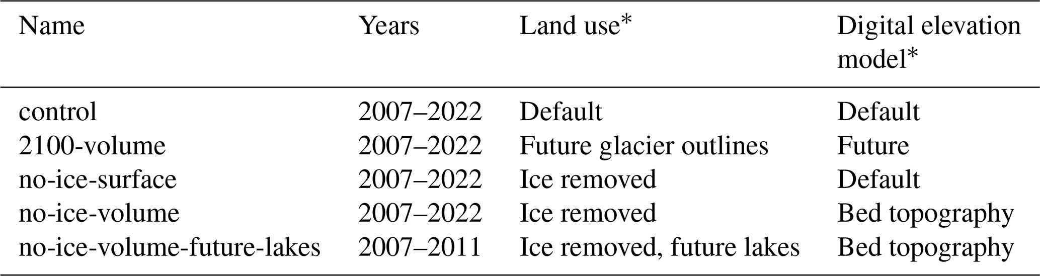
^∗ Details of default current and future land use data and digital elevation models are described in the text.

To test the impact of future glacier changes on local weather and climate, we use ice extent and elevation from high-resolution glacier projections for Jostedalsbreen for 2071–2100 under the RCP4.5 emission pathway (“Future glacier outlines” in Table 1) from Åkesson et al. (2025). Nearby smaller glaciers and ice patches are not part of the glacier projections from Åkesson et al. (2025). Such small glaciers are, however, expected to disappear in a warming climate (e.g., Van Tricht et al., 2025), and are therefore only included in the control experiment. We also include ice-free experiments (“Ice removed” in Table 1), to assess the meteorology and climate without a glacier present in the area. When ice-covered grid cells are removed in WRF, the new land use category is specified as “barren or sparsely vegetated”. In one experiment, we also include potential future lakes (“Ice removed, future lakes” in Table 1) from Gillespie et al. (2024a) covering 61 grid cells that are ice-covered in the control experiment. An overview of the experiments is presented in Table 1.

Along with the modifications in land surface type, surface elevation in WRF was for some experiments updated based on the ice surface in 2100 (“Future” in Table 1) from Åkesson et al. (2025), with a 100 m grid spacing, or the bed topography (“Bed topography” in Table 1) from Gillespie et al. (2024a), with a 10 m grid spacing. In these experiments, the updated terrain model was confined to a polygon area surrounding the ice cap and did thus not cover the entire inner domain. The polygon shaped terrain models were therefore bilinearly resampled to the grid spacing of the default terrain model before merging the two terrain models. In the transition zone between these two terrain models, Gaussian filtering was applied to smooth the edge. Since the grid spacing of the terrain model is only 50 m and considerably smaller than the 1 km model grid spacing, this preprocessing of the terrain models has likely negligible impact on the simulations. However, the preprocessing of the modified digital elevation model in these two experiments resulted in some differences in the terrain outside the ice cap compared with the control simulation (Fig. A1). The mean elevation change outside the ice cap is 3 m for both the 2100-volume and the no-ice-volume experiments compared to the control experiment, with a standard deviation between 20 and 21 m, respectively. While this elevation change is artificial, of unclear origin, and is expected to unintentionally cause lower temperature and more precipitation when the terrain is lifted (and vice versa), the elevation change is at least one order of magnitude smaller than the mean elevation change of 38 and 81 m over the ice cap for the 2100-volume and the no-ice-volume experiments, respectively. Moreover, as these artificial differences nearly cancel each other on scales of some 10 km², we argue that the regional climate from these sensitivity experiments can still be explored.

We use the same physical schemes as Haualand et al. (2025), including the Thompson microphysics scheme (Thompson et al., 2008), the RRTMG scheme for longwave and shortwave radiation (Iacono et al., 2008), the horizontal Smagorinsky first-order scheme for horizontal diffusion (Smagorinsky, 1963), the Mellor-Yamada-Nakanishi-Niino Level 3 (MYNN3) scheme for the boundary layer and surface layer (Nakanishi and Niino, 2009), and the Noah land-surface model (Koren et al., 1999; Ek et al., 2003). These were found to be optimal for representing temperature, wind speed, and precipitation in this region (Haualand et al., 2025), despite limitations such as no or simple representation of glacier dynamics and snowpack characteristics that sometimes result in cold biases near snow and ice surfaces (Letcher et al., 2024; Abolafia-Rosenzweig et al., 2025). In this model configuration, permanent snow and ice surfaces are assigned an albedo of 0.55 when the seasonal snow cover is absent, with the albedo increasing to up to 0.8 when snow accumulates in the grid, depending on the estimated snow cover fraction. For most processes, a few days of spin-up was enough, but since the simulation starts with no snow cover, a full winter season was needed to accumulate enough snow to establish a reasonable snow cover in the accumulation area at higher elevations before the first simulated summer in 2007.

Model validation was already performed by Haualand et al. (2025), but will be extended here due to a focus on longer time scales and larger spatial scales. Due to the model's limited capability to resolve weather station altitude, modelled temperature data is altitude-adjusted using a lapse rate of 0.5 K per 100 m, in line with Dutra et al. (2020).

3.2 Meteorological data for validation

3.2.1 Weather stations

Weather data used for model validation is collected from automatic weather stations (AWSs, triangles in Fig. 1, more details in Table 2) in the proximity of the ice cap and is provided by the Norwegian Meteorological Institute via the Norwegian Centre for Climate Services (2025) and the Norwegian Water Resources and Energy Directorate (2025). In addition, one PROMICE weather station (Fausto et al., 2021) was set up on the outlet glacier Nigardsbreen (NB) in June 2021, providing the only direct weather observations from a glacier surface in the area for the last 1.5 years of simulation time. To get more measurements from higher elevations close to the ice cap, we also use one private weather station at Steinmannen (SM) operated by the hydropower company Statkraft. All data from the weather stations are quality controlled by the providers. While smaller sporadic data gaps exist at most locations, large data gaps are limited to large parts of 2014–2016 and 2020–2025 at Flatbreen (FB) and 2019–2021 at Spørteggbu (SB), and data from these two remote stations are therefore interpreted with extra caution. The station in Jostedalen (JD) was moved to a nearby location in Mjølversgrendi (MG) in 2020, but these stations are here treated as two independent stations due to changes in topography and land use.

Table 2 Overview of automatic weather stations shown in Fig. 1. More details can be found in the text.

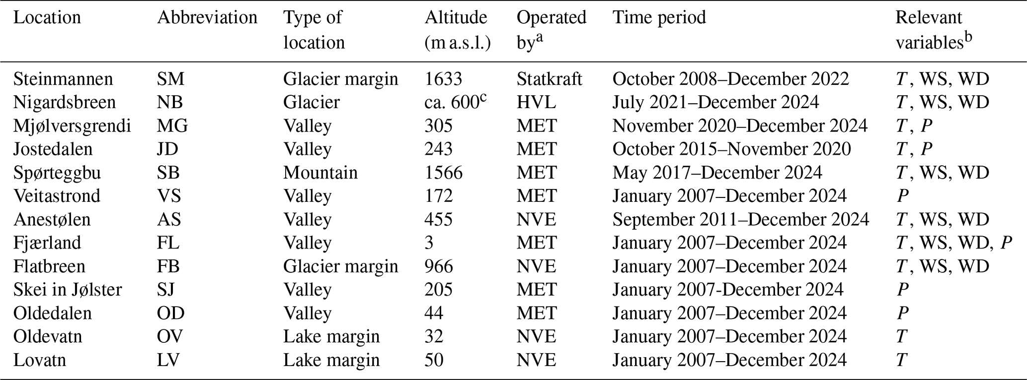
^a HVL: Western Norway University of Applied Sciences; MET: Norwegian Meteorological Institute; NVE: Norwegian Water Resources and Energy Directorate (official abbreviations refer to the Norwegian names). ^b T: temperature, WS: wind speed, WD: wind direction, P: precipitation. ^c The elevation of the glacier station has varied by ca. 50 m due to ice movements.

3.2.2 Indirect weather data from snow density measurements

With no direct measurements of precipitation at the ice cap and at higher elevations near the ice cap, snow density profiles at the ice cap were used for validating winter precipitation in the accumulation zone of the ice cap. Based on these annual snow density measurements at upper parts of the outlet glaciers Nigardsbreen and Austdalsbreen, the accumulated snow water equivalent for each winter season is estimated and compared to modelled values from September to May. Despite some uncertainties related to the impact from liquid precipitation and melting during the extended winter season as well as snow drift that is not accounted for in the model, these estimates are currently the best available indications of precipitation at higher elevations of the ice cap. Further details about the measurements can be found in the report by Andreassen et al. (2025).

4 Results and discussion

4.1 Validation

Using a nearly identical model setup as in this study, Haualand et al. (2025) reported in general good model performance of wind and temperature in early autumn around Nigardsbreen (see NB and MG in Fig. 1), one of the glacier-valley systems at Jostedalsbreen. Their main challenge was a model underestimation of 2 m air temperature over the glacier, which was probably related to too low vertical resolution to sufficiently represent the very stable layer above the ice as well as too high modelled albedo of ice surfaces resulting in too much surface reflection and lower temperatures than in reality. Extending this validation to a longer period and larger area, monthly and annual temperature, precipitation, and wind are here compared to local observations for the control experiment with glacier outlines from 2019.

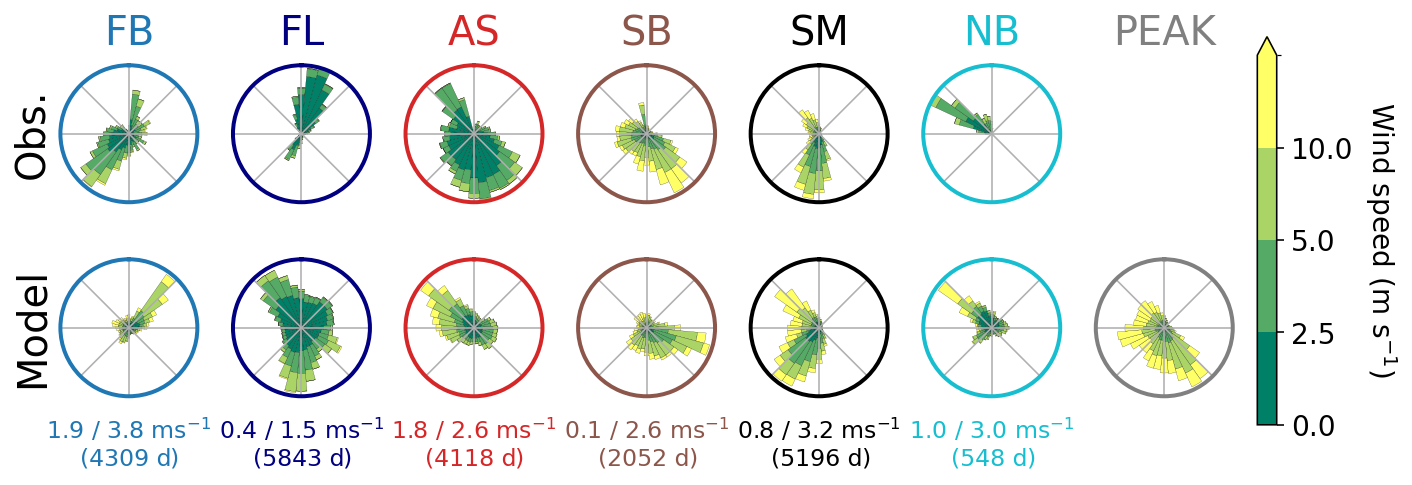
Figure 3 Wind roses based on observations (upper panel) and model output (lower panel) for selected AWS locations colored by the same color as the stations in Fig. 1. The wind rose with grey edge color is the only location that is not associated with an AWS and is located at the highest point on the ice cap. Numbers below each wind rose pair represent mean model bias and absolute error, respectively, followed by the number of days used in each wind rose pair where both observations and model output exist.

Modelled precipitation is well represented with a relative error of 1 %–9 % at most stations except a large overestimation of 49 % at Oldedalen (OD; Fig. 2). The model performance of precipitation at Oldedalen is location-sensitive and likely related to the smoothed model topography and an overestimation of spillover effects in the lee of the prevailing southerly winds (see wind roses from SB, SM, and PEAK at higher elevations in Fig. 3). The large overestimation in Oldedalen is also associated with, but not limited to, some extreme weather events (not shown). While no direct measurements of precipitation exist at the upper ice cap, modelled snow at high elevations on the ice cap is in good agreement with snow estimates from snow density profiles (stars in Fig. 2), despite the uncertainties related to wind drift, rain, and melting processes. Modelled snow over the entire ice cap (Fig. A2) is also in good agreement with modelled winter surface mass balance by Sjursen et al. (2025). Finally, the high modelled precipitation at the upper ice cap is comparable to estimated precipitation by Tveito (2021) who used an elevation dependency of 7 %/100 m to produce spatially interpolated gridded maps of precipitation.

Table 3 Mean absolute and bias errors of modelled mean monthly temperature for relevant stations in Fig. 1.

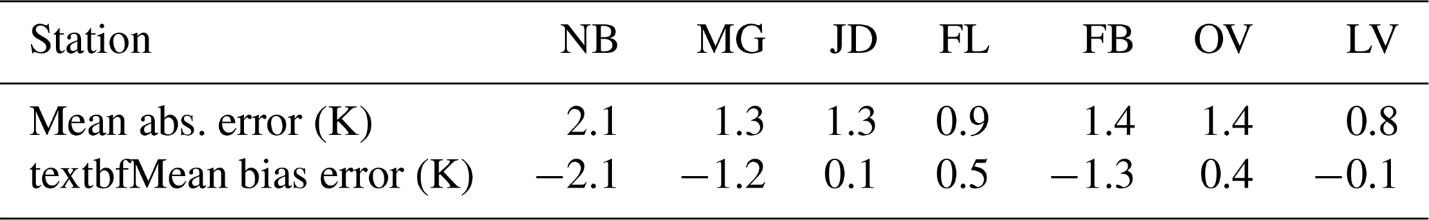
Modelled temperature is also adequately represented given the complexity in terrain and land use, with a mean absolute bias between 0.8 and 1.4 K after altitude correction at the six off-glacier AWSs (MG, JD, FL, FB, OV, and LV; see Fig. 1) that are most relevant for the ice cap (Table 3). At the only glacier station (NB), the bias is −2.1 K, which is consistent with the underestimation at this station reported by Haualand et al. (2025) and expected from the general challenge of numerically representing the shallow and very stable layer near the ice surface and the typically low albedo of glacier ice. Some of this underestimation may also be related to inaccurate temperature observations due to snow accumulation around the station peaking in spring and leading to a measurement height down to ca. 70 cm above the snow surface (not shown). The largest biases at the off-glacier stations are found in late spring at the stations near this glacier station in Jostedalen (MG and JD; Fig. 4), which are likely related to wrong timing of the snow melt in the snow-rich valley. Overall, the temperature at the off-glacier stations is best represented in the summer and winter months, while the temperature of the glacier station is best represented in early winter.

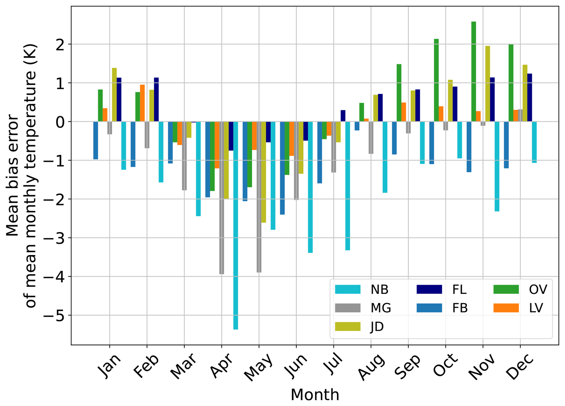
Figure 4 Mean bias error of mean monthly temperature sorted by month for the seven most relevant AWSs in Fig. 1.

Wind data from the simulation period is limited to six relevant weather stations around the ice cap (NB, SM, SB, FL, FB, and AS; see Fig. 1), all located in complex terrain that is only partly resolved by the model. Therefore, the simulated wind direction at these locations is not always well represented, particularly at one station located on top of a moraine near a glacier and a lake (FB, Fig. 3), where local variations in topography and land surface type are large. Other locations where local wind conditions are not well represented are two valley stations located near a fjord and a lake (FL and AS) in winter, which are frequently associated with cold air pooling and land-sea breezes. At all stations, the modelled wind speed is too high (see errors in Fig. 3). This overestimation is partly due to comparing winds at different altitudes above ground, as modelled winds are estimated at 10 m, while most observed winds are measured around 3 m or sometimes lower due to snow accumulation around the remote stations in winter. Furthermore, overestimation is a well known challenge in numerical weather prediction and may be attributed to lacking sheltering effects by the smoothed topography and potentially unresolved temperature inversions at night and in winter. Wind conditions are in general much better represented at two mountain stations around 1600 m a.s.l. (SB and SM) and at the glacier station (NB), probably due to less local variations in topography and land surface type.

Overall, despite some expected challenges of representing local phenomena like cold air pools and topographically forced wind systems at this resolution, we find that the model represents important non-local wind conditions as well as temperature and precipitation over multi-year periods well.

4.2 Sensitivity experiments

4.2.1 Meteorological effects of glacier recession and disappearance

The sensitivity experiments related to glacier recession or complete disappearance result in higher 2 m air temperature (hereafter referred to as temperature) and less precipitation over the original ice cap, and negligible temperature changes and varying precipitation changes outside the ice cap compared to the control experiment (Figs. 5a–c and 6a–c). These changes are detailed in the following.

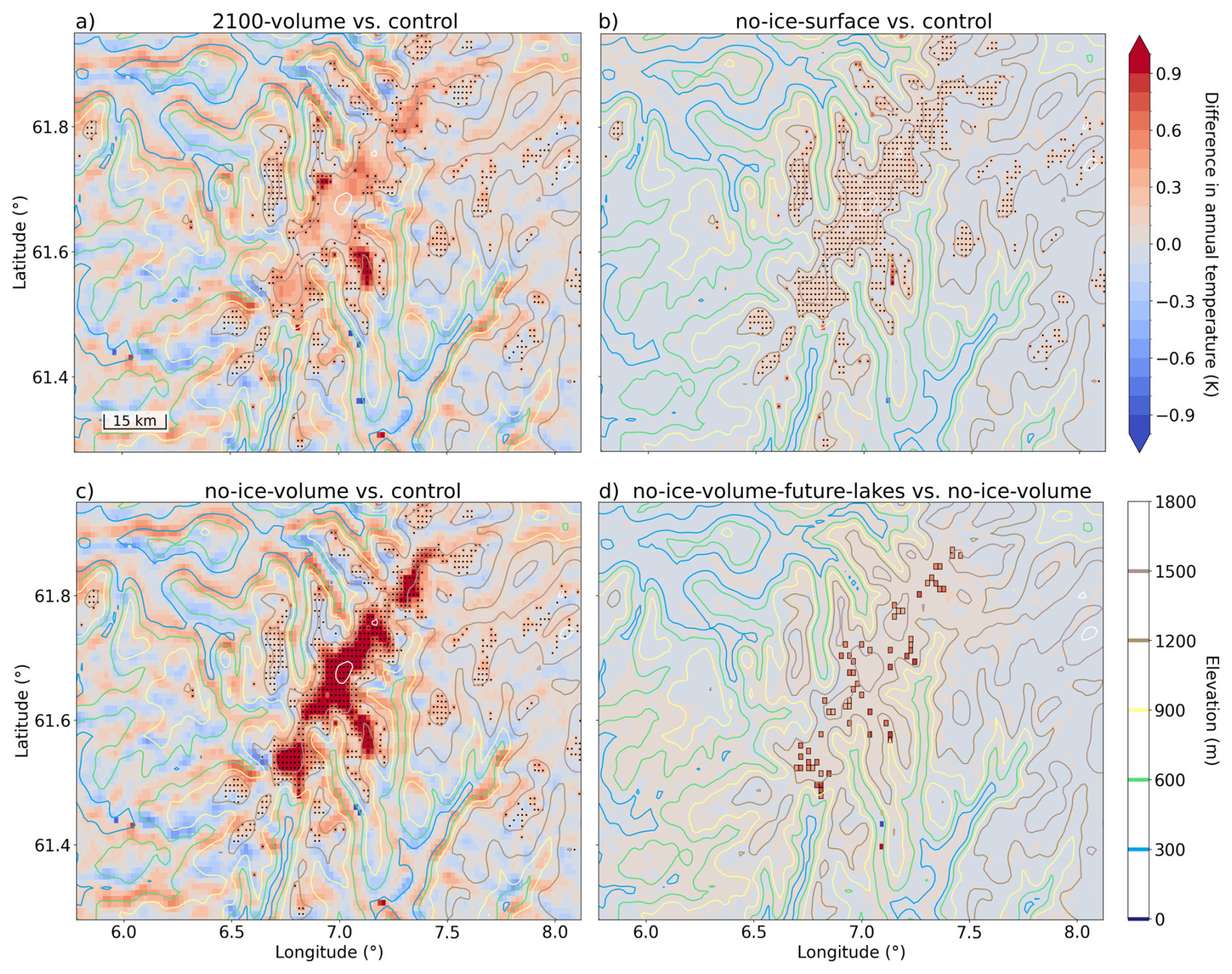
Figure 5 Difference in modelled mean annual temperature between (a) the experiment with ice volume for 2100 and the control experiment, (b) the experiment with no ice surface and the control experiment, (c) the experiment with no ice volume and the control experiment, and (d) the experiment with no ice volume and future lakes and the experiment with no ice volume but no future lakes. The differences are taken for 2007–2022 except in panel (d) where the differences are only for 2007–2011. Differences in ice and lake surfaces between the two experiments are denoted by black dots and blue frames, respectively, in each relevant grid cell. Colored contours show model elevation every 300 m for the control experiment in panels (a)–(c) and for the experiment with no ice volume in panel (d).

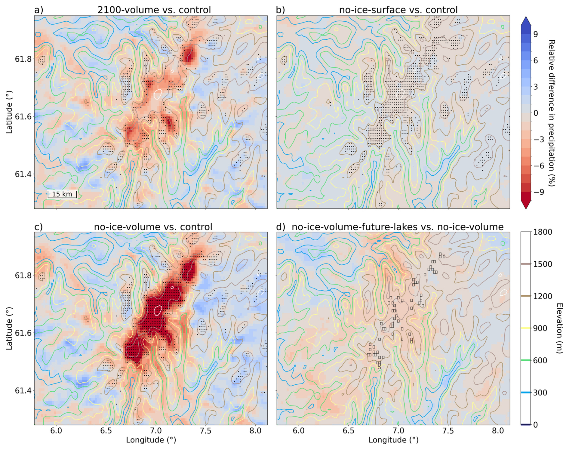
Figure 6 Same as Fig. 5 except that shading shows relative difference in modelled mean annual precipitation instead of difference in modelled mean annual temperature.

When the ice surface is removed, but the elevation is unchanged (no-ice-surface experiment), changes in temperature, precipitation, and wind are very small, with less than 0.5 K increase in temperature (Fig. 5b) and less than 1 % reduction in precipitation (Fig. 6b) over the ice cap. The temperature increase is robust and nearly constant across the ice cap and likely mainly related to the albedo feedback, where darker surfaces underlying the ice absorb more solar heating, as well as the possibility to reach skin temperature above 0 °C when the ice surface is removed. In contrast, the precipitation changes are varying in space, particularly outside the ice cap, but are nearly negligible and will therefore not be further physically interpreted.

When ice removal is accompanied by corresponding surface-lowering (no-ice-volume experiment), changes in temperature and precipitation are much larger, with up to 2 K increase in temperature and up to 20 % reduction in precipitation over the ice cap compared to the control experiment (partly shown in Figs. 5c and 6c). The added increase in temperature is largest where the elevation change is largest and is directly associated with the lowering of the terrain and the associated increase in surface pressure. The warming over some valley glaciers (particularly Tunsbergdalsbreen, Fig. 1) reduces slightly in winter (not shown), which is probably related to cold air pooling that frequently occurs in this region at this time of the year. The local patterns of cooling and warming outside the ice cap are mainly associated with the artificial adjustments of the model terrain mentioned in Sect. 3.1 and are therefore not further interpreted.

Along with the overall warming in the no-ice-volume experiment, the annual snow-to-rain ratio decreases over the ice cap, resulting in a more than twice as large absolute reduction in snow than reduction in rain over the ice cap when the ice volume is removed (not shown). Away from the ice cap, changes in precipitation are both positive and negative and mostly between −4 % and 4 %, with a tendency of slightly wetter climate on the eastern side of the ice cap where storms are normally weaker than on the coastal western side of the ice cap (Fig. 6c). These changes, which occur several 10 km away from the removed ice cap, demonstrate that the impact on precipitation is regional and that the changes are related to less orographic lifting where the terrain has been lowered and thus more moisture available for precipitation further inland. In contrast, on the coastal (western) side of the ice cap, which is where most of the precipitation in the region comes from, the negative and positive precipitation response nearly cancel, indicating minimal net regional impact upstream of the changed topography. The local pattern of changes in precipitation on the western side is likely mainly related to artificial adjustments of the model terrain mentioned in Sect. 3.1 and should therefore not be evaluated on spatial scales covering individual valleys and mountain ridges.

A full removal of the Jostedalsbreen ice cap is unlikely to occur in the 21st century (Åkesson et al., 2025). The smaller ice cap projected for the end of the century (2100) for a moderate emission scenario (RCP 4.5) presents an opportunity to test the impact of ongoing glacier recession on the local and regional climate. This experiment (2100-volume), shows that, compared to the no-ice-volume experiment, the magnitude of the changes in temperature and precipitation are reduced across nearly the entire ice cap, particularly at higher elevations where there is naturally less ice removal (Figs. 5a and 6a). The largest changes in temperature and precipitation are in this experiment at relatively low elevations where there is currently thick ice that is projected to thin or melt away completely over the next decades, such as at the lower parts of Tunsbergdalsbreen (“TB” in Fig. 1). Here, the absolute increase in temperature and relative decrease in precipitation are up to 0.7 K and 9.9 %, respectively, but the signal reduces with elevation and there is nearly no change in temperature and precipitation at some higher elevations of the ice cap.

While the increase in temperature associated with future ice loss arrives solely due to changes in elevation and land surface type, the effect of ice loss on temperature will in a more realistic scenario accounting for climate change likely amplify the warming projected by most regional climate models. In contrast, the decrease in precipitation due to ice loss could counteract, and in some places overcompensate for, the projected 4 % regional increase in precipitation averaged from a large set of climate models that are based on the same moderate emission scenario as the projected ice loss (RCP 4.5; Dyrrdal et al., 2025). This finding may have global implications, indicating that regions with extreme glacier recession where orographic precipitation is important may become drier in the future despite a projected increase in precipitation from other effects of global warming. However, large uncertainties in the study design and the robustness of this finding call for more research including coupled models that explicitly represent feedback effects between the glacier and the atmosphere. Such coupled models could clarify how reduced precipitation due to ice loss feeds back on glacier recession by reducing snow accumulation and ice melt related to rain. The net effect on glacier recession will depend on the spatial distribution of the change in precipitation. If reduced accumulation dominates over reduced melting, ice loss will likely amplify, resulting in a positive feedback effect between glacier evolution and precipitation.

4.2.2 Meteorological effects of new future lakes

Our findings related to glacier recession show that impacts by changes in land use are more than one order of magnitude smaller than those related to changes in elevation. One of the reasons for the minimal effect from changes in land use are likely due to insufficient removal of seasonal snow related to lacking glacier dynamics in the model, which leaves some ice-free surfaces artificially snow covered. This additional snow covering increases the albedo and opposes the warming effects resulting from removal of ice surfaces. Nevertheless, while the additional snow suggests that warming effects due to albedo changes are underrepresented by the model, these potential errors may partly cancel with errors related to glacier surfaces falling into the same land surface category as snow. In such a combined snow and ice category, the albedo of glacier surfaces is typically too high and therefore decreasing too much when glaciers recede.

Further changes in albedo occur along with modifications in moisture fluxes between the surface and the atmosphere when future lakes are added (“no-ice-volume-future-lakes”). These new lake surfaces represent a change in land use in 7 % of the glacier grid cells that were removed when the entire ice cap is removed. The addition of new potential future lakes when the ice is removed results in further warming and drying of the area where the ice is gone, when compared to the corresponding experiment without future lakes (Figs. 5d and 6d). However, the temperature changes are mainly restricted to the lake grid cells, where they are around 1 K, and are below 0.1 K elsewhere (Fig. 5d). The reduction in precipitation is also weak (less than 4 %, Fig. 6d) and mainly confined to spring, summer, and fall (not shown). This indicates that inclusion of future lakes has little impact on regional climate, though large uncertainties exist due to model limitations.

Glacier disappearance and formation of new lakes are not realistic without associated changes in climate. In this relatively short study period from 2007 to 2022, where climate is nearly unchanged, meaningful interpretation of the impact of future lakes is limited due to the unrealistically cold environment where these future mountain lakes exist. In this cold environment, snow accumulates in the surroundings of the new lakes during large parts of the year, but since this configuration of WRF does not allow for snow accumulation over lakes, there will sometimes be large contrasts of surface temperature across the land and lake surfaces. In reality, most of the new lakes would form in a climate that is considerably warmer than present, because several hundred meters of ice need to melt. In such a warmer climate, there will be less snow accumulating around the lakes, which likely results in a modified impact by future lakes. Therefore, the increase in temperature and precipitation by future lakes found in this study should be further studied in a coupled model accounting for climate change and interactions between glacier mass balance and atmospheric drivers. Such a coupling would also strengthen the robustness of the findings related to ice removal.

4.2.3 Importance of large-scale wind direction

Weather and climate around Jostedalsbreen is strongly governed by the dominating upper-level wind direction, which is normally from between southeast to west (clockwise, Fig. 3). To explore the model sensitivity of changes in temperature and precipitation to large-scale weather patterns, we define the daily wind regime by sorting the wind direction at the top of the ice cap (labeled “PEAK” in Fig. 3) into four wind direction bins ±45° from north (“N”), east (“E”), south (“S”), and west (“W”) before finding the most frequent wind direction for each day.

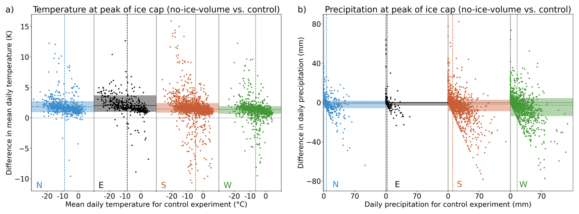
Figure 7 (a) Daily mean temperature and the difference in daily mean temperature between the no-ice-volume experiment and the control experiment, all taken at the highest point of the ice cap and sorted into four wind direction bins (northerlies, easterlies, southerlies, and westerlies). Dashed vertical and horizontal lines show the mean x and y values for each wind direction bin, respectively. Partly transparent colored shading highlights the interdecile range (between the 10th and 90th percentile) for the differences along the y-axis. (b) Same as panel (a) but for daily precipitation instead of daily mean temperature.

In line with the common track of cyclones from the North Atlantic ocean toward western Norway, the wettest days are associated with wind from south and west (orange and green dots and dashed vertical lines in Fig. 7b, respectively). These are also the wind directions with the largest change in precipitation after removing the Jostedalsbreen ice cap (the no-ice-volume experiment), with a mean difference in daily precipitation of −1.5 and −2.6 mm on days with southerlies and westerlies, respectively (dashed horizontal lines in Fig. 7b). While these daily mean values may seem small, they are statistically different from zero, with p-values below 10⁻⁵ in a one-sample t-test. Furthermore, these mean values account for a large number of dry days where no change in precipitation occurs and increase significantly when accounting only for wet days. For example, accounting only for days with more than 5 mm daily precipitation yields a mean daily change of −5.7 and −6.0 for southerlies and westerlies, respectively (not shown). Less change in precipitation is found during the generally drier northerlies and easterlies (blue and black dots in Fig. 7b), with easterlies actually contributing to slightly wetter weather during glacier recession, though only with a mean daily change of 0.2 mm (black dashed horizontal line). However, also for these wind directions, the change in precipitation gets more negative when accounting only for days above a certain threshold in daily precipitation.

In contrast to the change in precipitation, the average absolute change in temperature is largest during easterlies (black dashed horizontal line in Fig. 7a). This is the wind direction associated with the coldest air masses in winter, due to the continental cooling of air on the eastern side of Jostedalsbreen. Due to the high mountains in east, this wind direction is ideal for foehn wind events, and the enhanced warming during easterly wind conditions may therefore be a result of increased lee-side dry adiabatic warming over Jostedalsbreen when the ice thins and the terrain is accordingly lower (Temme et al., 2020). Along with enhanced warming during easterlies, there is generally more warming from glacier disappearance on cold days compared to warm days (Figs. 7a, A3a, and A4a), suggesting that temperature variability over the ice cap will be smaller when the ice cap gets thinner or is completely melted away.

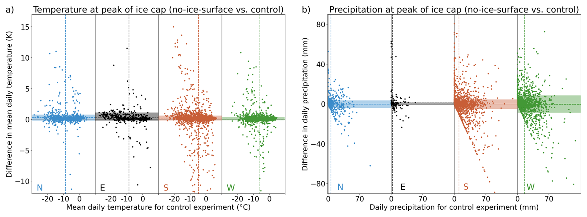
Similar qualitative impact from wind regimes are found for other locations, including locations adjacent to the current ice extent of the Jostedalsbreen ice cap. Also, the overall role of wind regimes does not change remarkably when comparing the other sensitivity experiments related to glacier recession to the control experiment (Figs. A3 and A4), although most of the mean differences in temperature and precipitation at the peak of the ice cap are smaller and less sensitive to wind regime, as expected from the smaller general differences over the entire ice cap (Figs. 5 and 6). The most notable changes for these other sensitivity experiments are that the increase in precipitation during easterlies gets larger and that the warming during easterlies reduces more than during other wind regimes (Figs. A3 and A4). The weaker role of easterlies for the temperature increase is likely because of no or very small reductions in the elevation at the peak of the ice cap for these two experiments, as opposed to the no-ice-volume experiment, resulting in little additional warming effects from easterly foehn winds. However, as the mean changes in temperature and precipitation in these other sensitivity experiments are small and not always statistically different from zero, these interpretations should not be given much weight. Instead, we focus on the overall impacts on temperature and precipitation from glacier recession, which are mostly qualitatively similar at all wind directions, though easterlies contribute relatively more to the increase in temperature when the entire ice cap is removed, while westerlies contribute relatively more to the decrease in precipitation.

4.3 Perspectives and feedback effects between glaciers and regional climate

Our findings of higher temperature and less precipitation due to glacier thinning suggest a modified view of the future climate over the Jostedalsbreen ice cap. While projected regional warming is expected to be amplified by feedbacks from glacier recession, precipitation might not increase as much as regional climate models predict if accounting for glacier thinning. Despite this counteracting effect on precipitation trends from glacier recession, trends in snowfall remain negative in both our study and in future regional climate projections (Dyrrdal et al., 2025). These opposing trends in snowfall and precipitation are due to increased temperature and highlight that changes in snowfall are dependent on the change in the interplay between both precipitation and temperature. Therefore, uncertainties in future snowfall are in general higher than those of the individual changes in temperature and precipitation, particularly at high elevations where snowfall is common. Our findings strengthen our confidence in the predicted future decline in snowfall and suggest in general that accounting for changes in glacier geometry in climate models can improve future projections of regional climate and their feedback on glacier recession.

Improvements in climate projections due to inclusion of glacier recession are expected to be largest over the ice cap where the climatic response is strongest (Figs. 5 and 6). As the horizontal extent of substantial elevation changes over the ice cap is covering some 100 km² in the 2100-volume and no-ice-volume experiments (not shown), impacts of glacier recession on temperature and precipitation over and near the ice cap should be possible to resolve in regional climate models. Away from the ice cap, the response is weaker and varies in space between positive and negative values and is likely more uncertain. Still, valleys directly connected to the ice cap tend to be associated with the same climatic response as the overall ice cap. This indicates that our findings are robust in areas several kilometers beyond the glaciated regions where agriculture and other human activity take place.

In a global perspective, we expect that the range, magnitude, and sign of the climatic response to glacier recession depend on the thickness and extent of the receded ice, the climate zone, and the importance of topography for orographic lifting and local atmospheric circulation. For example, in studies where monsoon systems play an important role for atmospheric circulation, glacierised regions were associated with reorganisation of local convection and more moisture transport and precipitation when the glacier surfaces were removed (Ren et al., 2020; Lin et al., 2021). Such an increase in precipitation is opposite of the reduced precipitation found in this study. In better agreement with our findings, Salerno et al. (2023) reported reduced precipitation near receding Himalayan glaciers and argued that a potential reason could be a strengthening of glacier winds and associated reorganisation of local wind convergence. It remains an open question if the role of elevation changes associated with glacier recession could play a role also at this site. Overall, studies on local atmospheric impacts by glacier recession remain limited, particularly because no or few studies explicitly account for changes in elevation. More research including elevation changes and covering various types of glacier-atmosphere systems and climate zones would allow for a systematic investigation of how the impacts of glacier recession differ globally.

More research is also needed to evaluate the two-way interactions between receding glaciers and a changing atmosphere. The overall warming and associated reduction in snow by glacier recession found in this study suggest that glacier recession will accelerate in the future through a positive feedback effect due to more melting of ice as well as less snow in the accumulation area (Fig. 8). This acceleration may come on top of increased melting due to weaker glacier winds (Haualand et al., 2025; Shaw et al., 2025). The coupling between glacier mass balance and atmospheric drivers has been found to be important for the surface energy balance and related surface processes (e.g., Collier et al., 2013; Eidhammer et al., 2021; Sauter et al., 2026). However, a two-way coupling over time is computational expensive, and coupled model simulations have therefore typically neglected changes in glacier geometry and dynamics and been limited to time scales with little climate change. Accounting for this coupling in longer climate simulations will likely improve the timing of glacier recession and the associated natural and societal consequences.

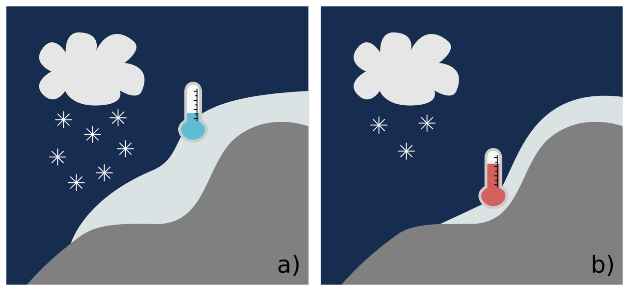
Figure 8 Conceptual illustration of the main findings of this study, where glacier recession from panel (a) to panel (b) is associated with increased surface temperature and reduced snowfall due to lower topography.

5 Conclusions

The impact of glacier recession and disappearance of the Jostedalsbreen ice cap in western Norway on regional climate is studied in the WRF model by modifying land surface type and elevation over the ice cap for the period 2007–2022. We draw the following conclusions.

1. Glacier recession results in warming and less precipitation over the ice cap (Fig. 8). Most of the reduction in precipitation is attributed to reduced snowfall.

2. Changes in surface temperature and precipitation are mainly a result of lowering of the terrain when ice melts and are related to higher surface pressure and less orographic lifting.

3. The warming from glacier recession is strongest during easterlies due to increased influence from foehn wind. Reduction in precipitation is strongest during westerlies and southerlies due to less orographic lifting of moist air masses from the ocean.

4. While the increase in temperature may accelerate projected regional warming, the decrease in precipitation over the ice cap may compensate for some or all of the projected increase in precipitation in regional climate models of the area around the Jostedalsbreen ice cap.

5. The warming and reduced snowfall by glacier recession suggests accelerated glacier recession and a positive feedback effect between glacier recession and regional climate change.

While this study focuses on the direct impact of vanishing ice on regional climate, our findings should be tested in coupled models accounting for changes in both glacier mass balance and the atmosphere over longer time periods. A better representation of snowfall will influence surface-atmosphere interactions, glacier recession, and the associated changes in topography and orographic processes. The impacts from glacier recession should also be explored in other glacier environments ranging from small glaciers to large ice sheets and in other climatic environments where orographic precipitation and local wind patterns play a different role. In particular, more studies should include the direct impact by glacier thinning. Our findings have relevance for glacier mass balance as well as climate adaptation related to agriculture, hydropower, tourism, and biodiversity around glaciated landscapes.

Appendix A: Supporting figures

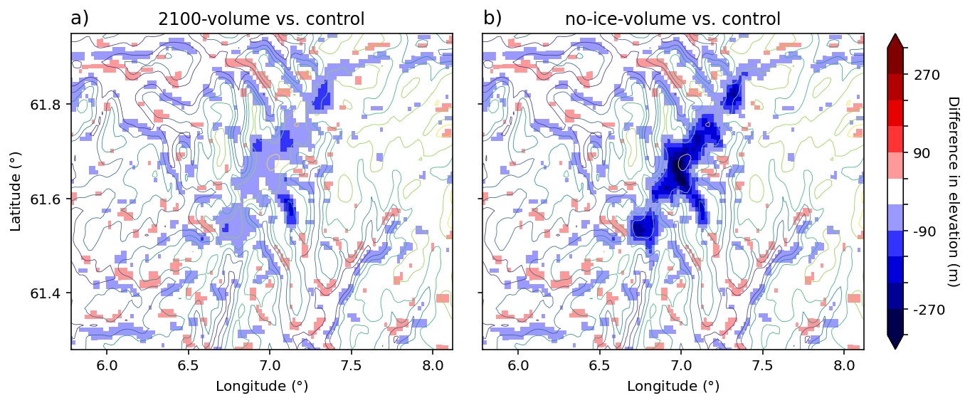
Figure A1 Difference in model elevation between (a) the 2100-volume experiment and the control experiment and (b) the no-ice-volume experiment and the control experiment. Colored contours show model elevation every 300 m for the control experiment.

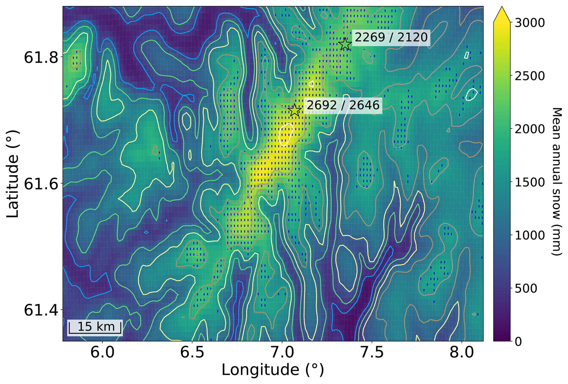
Figure A2 Mean annual snowfall from model (shading) and locations for snow density measurements used to estimate mean snow water equivalent for September–May (stars) for 2007–2022. Numbers next to colored stars highlight the corresponding modelled+observed values of snow water equivalent in mm, respectively. Colored contours show model elevation each 300 m. Each grid cell with a permanent ice/snow surface in the control run is marked by a blue line.

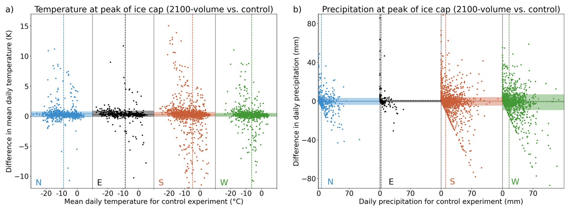
Figure A3 (a) Daily mean temperature and the difference in daily mean temperature between the 2100-volume experiment and the control experiment, all taken at the highest point of the ice cap and sorted into four wind direction bins (northerlies, easterlies, southerlies, and westerlies). Dashed vertical and horizontal lines show the mean x and y values for each wind direction bin, respectively. Partly transparent colored shading highlights the interdecile range (between the 10th and 90th percentile) for the differences along the y-axis. (b) Same as panel (a) but for daily precipitation instead of daily mean temperature.

Figure A4 Same as Fig. A3, except for differences between the no-ice-surface experiment and the control experiment.