Intraseasonal prediction of monthly storminess in the North Sea with the ACE2 atmospheric emulator and Random Forests

This research explores the predictability of seasonal storminess in the North Sea using machine learning methods and the weather model emulator ACE2, focusing on how the stratosphere and upper troposphere influence winter storms. Understanding the drivers of winter storminess is essential for improving sub-seasonal prediction skill in regions strongly affected by extratropical cyclones. Using ERA5 reanalysis data (1940–2024), we built a storminess index based on storm-event frequency, examined its relationship with large-scale atmospheric fields, and explored its predictability on seasonal timescales.

We aim to predict North Sea storminess using two approaches: one based on the ACE2 climate emulator and another on the Random Forest machine learning algorithm. The ACE2 simulations show that by decreasing the stratospheric temperature and increasing the wind speed on 1 December, we can increase the emulated mean January surface wind speeds by about 0.5–3 m s⁻¹ across much of the North Sea. Similar sensitivity emulations initialised at the start of other months, e.g. 1 November, failed to produce a meaningful response in the ensuing month. This suggests a dynamic link between early-winter stratospheric conditions and increased mid-winter surface storminess.

For the Random Forest regression model, monthly means of air temperature, zonal wind at 70 hPa, and geopotential height at 200 hPa were used as predictors after dimensionality reduction using Principal Components Analysis (PCA). The highest skill was obtained when predicting January storminess from December fields, with a correlation of about 0.55–0.60, while predictive skill was substantially weaker and sometimes negative for other month-to-month predictions.

This seasonal predictability pattern, derived from both the ACE2 emulations and the Random Forest model, follows the seasonal cycle of the polar vortex's average intensity. The circumpolar westerly jet strengthens from autumn and peaks in winter, when predictability is highest. This higher skill is likely linked to stronger stratosphere–troposphere coupling that peaks in late December and extends until mid-February, as polar vortex anomalies develop and begin to descend toward the surface. Both indicate that the seasonal predictability of storminess peaks in mid-winter, with a predictability lead time of about 4 to 6 weeks. It fades for the earlier and late winter periods.

We found that North Sea storminess, measured as the monthly or seasonal number of storms, is not statistically correlated with storminess in any other region of the globe. This suggests that although individual seasons or months may show increased storminess over large areas, the statistical predictors of North Sea storminess must have a small-scale regional character specific to the North Sea. We also found that the North Sea storminess shows no statistical persistence from month to month. This suggests that although individual winters may display North Sea storminess across all winter months, predictors of North Sea monthly storminess should also have a short-term subseasonal temporal scale. Together, these two findings indicate that sea-surface temperatures are not an adequate statistical predictor of North Sea storminess, although they may play a role in individual winters.

Overall, this research shows that stratospheric conditions play an essential role in shaping North Sea winter storminess and that machine learning methods can improve sub-seasonal predictions in this region.

1 Introduction

Seasonal climate prediction typically focuses on forecasting mean seasonal values a few months ahead, using either ensembles of initialised simulations from Earth System models or predictors identified for statistical prediction schemes. Although forecasts of seasonal means can undoubtedly be very important for many economic and societal sectors, probabilistic predictions of just the frequency of specific types of extremes can also be beneficial and more skilful, as they focus on a specific range of the probability distribution. The North Sea, a shallow sea in Western Europe connected to the North Atlantic, is strongly exposed to winter wind extremes, which affect shipping and impact the coast, causing storm surges, coastal flooding, and coastal erosion (Donat et al., 2011; Feser et al., 2014; Schade et al., 2025). In this study, we explore the possibility of predicting the stormy character of the winter months in the North Sea with a few months' lead time.

Surface winds in winter in the North Atlantic and the North Sea are statistically linked to the North Atlantic Oscillation (NAO), a dominant pattern of interannual climate variability in the North Atlantic sector that displays well-known teleconnections to near-surface temperature, sea-surface temperature (SST) and precipitation (Hurrell et al., 2003; McKenna and Maycock, 2022). Essentially, the NAO describes the strength of the mid-latitude zonal atmospheric circulation over the North Atlantic, as summarised by the seasonal mean air pressure differences between the Azores and Iceland (Hurrell et al., 2003), although other indices based on Principal Component Analysis of the North Atlantic sea level pressure field are also commonly used (Pinto and Raible, 2011).

Due to its dominant role in interannual winter climate variability in the North Atlantic-Western European sector, several studies have sought to identify seasonal precursors of the NAO state. Some of these studies have focused on the role of Tropical Atlantic (Wang et al., 2017; Sung et al., 2013) and Tropical Pacific SST (Sung et al., 2013). Regarding the state of the Tropical Pacific, previous studies have found that warmer temperatures, corresponding to an El Niño phase, tend to be associated with a negative NAO, colder North European winters, and wetter Western Mediterranean conditions. In contrast, the opposite phase, La Niña, is statistically associated with a positive NAO, with warmer North European winters and drier Western Mediterranean (Brönnimann, 2007). However, these links appear to be weak, non-stationary, and non-linear, and may also be modulated by the state of the Pacific Decadal Oscillation (Gershunov and Barnett, 1998). For example, the European winter 2025–2026, with a predominant La Niña state in the Tropical Pacific and a negative NAO, illustrates a clear counterexample. Other sources of predictability identified in model studies are the extent of Arctic sea-ice cover and the Quasi-Biennial Oscillation. Scaife et al. (2014) use a long-range forecast system to show that winter climate over the North Atlantic region, specifically the NAO, storminess, temperature, and wind speed, may now be highly predictable months in advance. However, the analysis also reveals that although forecast skill is significant, some key sources of predictability remain underrepresented, suggesting potential to improve long-range climate forecasting.

The NAO is more directly connected to the Arctic Polar Vortex in the lower stratosphere (Kidston et al., 2015), with a stronger winter vortex and a positive winter NAO tending to occur simultaneously on seasonal timescales. The typical westerlies in the lower stratosphere within the polar vortex can be disrupted by Sudden Stratospheric Warming (SSW) events. SSWs are intraseasonal events caused by the breaking of planetary-scale waves that propagate upwards from the troposphere (Baldwin et al., 2021), thereby modifying the vertical temperature profile and dynamically disrupting the lower stratospheric zonal flow. Kidston et al. (2015) explains how variations in the strength of the stratospheric polar vortex strongly influence the tropospheric jet stream, storm tracks, and extreme surface weather. When the vortex weakens, especially during major SSWs, the tropospheric jet shifts towards the equator, increasing the likelihood of cold outbreaks, blocking, and extreme winter weather over Europe and North America. When the vortex strengthens, the jet shifts poleward, enhancing surface winds at midlatitudes. These downward impacts occur because wave-driven disturbances in the stratosphere modify mass, pressure, and eddy momentum in the troposphere, producing consistent surface responses from weekly to decadal timescales. Kidston et al. (2015) also highlights that stratospheric variability affects the ocean and provides significant skill for subseasonal-to-seasonal forecasts, making an accurate representation of the stratosphere also essential for reliable climate predictions and projections.

In addition, tropical Pacific SST variability influences the Arctic polar vortex and Northern Hemisphere circulation in a highly nonlinear way, with both El Niño and La Niña winters exhibiting enhanced SSW frequency relative to neutral conditions (Butler and Polvani, 2011). Previous work suggests that the apparent enhancement of SSW frequency during both El Niño and La Niña phases in reanalyses such as ERA5 may be influenced by the limited length of the observational record (Polvani et al., 2017). Using large hindcast ensembles, Ineson et al. (2024) show that this behaviour can arise by chance, and that with a larger sample size, a more linear ENSO–polar vortex relationship may emerge. This would be more consistent with the established impact of ENSO on boreal winter stratospheric circulation. ENSO teleconnections to the North Atlantic–European region also evolve seasonally: early-winter impacts are mainly tropospheric and project more strongly onto the East Atlantic Pattern (Thornton et al., 2022), while the stratospheric pathway becomes increasingly important later in winter, favouring a positive NAO signal (Ineson and Scaife, 2009). This seasonal evolution and multiplicity of pathways make it more difficult to identify the remote SST precursor of extreme winds in the North Sea, as the linkage is likely to occur through several pathways and be strongly nonlinear.

With this background, this study aims to assess the predictability of stormy winter seasons in the North Sea, a relatively small but economically important region for Western Europe. Storm surges cause a significant rise in coastal water levels, which can have substantial socio-economic consequences and, in extreme cases, may even result in fatalities. Furthermore, these extreme water levels, in combination with strong winds and long-lasting precipitation events, can severely impact onshore and offshore transport systems and their infrastructure (Kew et al., 2013; Schade, 2017). Winter storms are among the most damaging climate hazards in northwestern Europe, and the North Sea region is particularly exposed due to its frequent extratropical cyclones and strong winds (Donat et al., 2011; Feser et al., 2014). A better understanding of these storms and the ability to predict them a season in advance are crucial for coastal protection, offshore wind planning, and the management of climate-related risks.

A study by Krieger et al. (2024) has shown that seasonal forecasts of German Bight storm activity using the hindcast system of the Earth System model MPI-ESM can be improved by subsampling the ensemble of simulations according to their individual agreement between the simulated and observed air temperatures at the 70 hPa geopotential height level in September, 2 months before the target prediction month. The initial predictive power of the whole ensemble is weak due to a very large spread. Using 70 hPa temperature anomalies (September) and 500 hPa geopotential height anomalies (November) as filtering criteria, the authors select ensemble members that agree with a first-guess forecast. This subselected ensemble significantly boosts prediction skill by better capturing large-scale atmospheric patterns. Other studies have examined storm predictability using various methods, including dynamical modelling (Xie et al., 2021; Tian et al., 2024; Gao et al., 2024; Pu and Kalnay, 2018), mathematical modelling (Tian et al., 2024), data-driven machine learning (Gao et al., 2024), and dynamical modelling and data assimilation (Pu and Kalnay, 2018). In our study, stormy seasons are those with a higher frequency of stormy days (see Sect. 2). One prediction methodology used here is Random Forest, a machine-learning method for categorical classification or predicting a response variable from several predictors (Breiman, 2001). The technique can be augmented with Random Forest Regression (RFR), which increases the number of categories to cover a given output range using a specified number of bins. The method can capture strongly non-linear links between the predictor and the predictand. In our case, the predictand is the number of exceedances of extreme daily wind, and the predictors may include the temperature field in the lower stratosphere from the previous season or earlier months, although other predictors were also tested. The second method is based on the atmospheric emulator ACE2 (Watt-Meyer et al., 2025). This emulator has recently been used for seasonal NAO predictions in an ensemble of simulations that impose observed SST and sea-ice extent anomalies on 1 November and hold them constant through the forecast horizon (Kent et al., 2025). Here, we use the ACE2 emulator, to our knowledge, for the first time, by prescribing modified stratospheric initial conditions while otherwise using observed boundary conditions through the forecast horizon in an extended weather forecasting setting. The ACE2 emulator is a machine-learning-based emulator of atmospheric dynamics that can be trained on reanalysis data or climate simulation data. This emulator has been shown to replicate important characteristics of global atmospheric dynamics and its response to tropical SST forcing (see Sect. 3.2). The main characteristics of the atmospheric circulation in the Northern Hemisphere are also well replicated (Bellinghausen et al., 2026). In our study, we utilised the ACE2 model in sensitivity runs of 2 months' length, in which the initial conditions are modified to mimic patterns of lower stratospheric warming or cooling and a strong or weak lower stratospheric polar vortex. The simulated North Sea extreme winds are then compared with those from runs initialised with observed conditions. This approach follows a similar concept of utilising a minimalistic modelling framework, as in a recent study by Mouallem et al. (2025). While our study imposes stratospheric initial conditions to assess their downward influence, Mouallem et al. (2025) focused on the upward initiation of SSW events. Related studies have also used stratospheric nudging approaches to assess stratosphere–troposphere coupling. For example, Kautz et al. (2019) and experiments within the SNAPSI framework (Hitchcock et al., 2022; Dai et al., 2025) nudge the zonally symmetric component of stratospheric circulation anomalies toward prescribed (observed) states to quantify its influence on the troposphere. The SNAPSI simulations are limited to three polar vortex anomaly cases. While the zonally symmetric component may be particularly relevant for these cases, the limited sample size hampers a broader assessment of its role. Later in our study, we argue that, on average, the zonally symmetric component of the polar vortex is unlikely to be responsible for North Sea storminess, as the statistical spatial coherence length of seasonal storminess is highly regional, restricted to the North Sea. This lack of circumpolar spatial coherence suggests that the frequency of North Sea extremes is modulated by regional dynamics or asymmetric vortex configurations, such as displacement vs. split events, rather than solely by the average intensity of the zonally symmetric circumpolar jet.

After this introduction, the paper describes the datasets (Sect. 2.1) and the definition of storminess (Sect. 2.2) used throughout the analysis in Sect. 2. Section 3 provides preliminary considerations on potential predictors through an analysis of the spatio-temporal persistence of stormy winter months in the North Sea and subsequently presents the main statistical analysis used to identify suitable predictors. This section (Sect. 3) also introduces the ACE2 emulator (Sect. 3.2) and the Random Forest regression model (Sect. 3.3). The outputs of both the ACE2 emulator and the Random Forest regression model are presented in Sect. 4. Section 4.1 analyses the ACE2 output, including changes in the frequency of extreme wind events and a sensitivity analysis of the identified predictors. Section 4.2 presents the Random Forest regression results, with a particular focus on predictability across different months. The paper concludes with a discussion of limitations and future work (Sect. 5), followed by a summary and conclusions (Sect. 6).

2 Methods

2.1 Dataset

Atmospheric and oceanic variables for the period 1940–2024 were obtained from the ERA5 reanalysis, the fifth-generation global climate dataset produced by the European Centre for Medium-Range Weather Forecasts (ECMWF) (Hersbach et al., 2020). The ERA5 dataset is produced by reconciling historical observational data with atmospheric physics encapsulated in a weather prediction model to ensure a continuous and consistent global record across all variables. The data were retrieved at a horizontal resolution of 0.25°×0.25° (approximately 31 km) on 137 atmospheric levels, extending from the surface to 0.01 hPa. In this study, we analysed monthly averages of geopotential height (200 hPa), air temperature (70 hPa), zonal and meridional wind (70 hPa), as well as daily 10 m wind speeds (Hersbach et al., 2020).

2.2 Definition of storminess

To calculate the number of stormy days in each month, we first obtained the zonal and meridional daily wind speeds at 10 m height from the ERA5 reanalysis for that month. Daily wind speed was computed from these components, and a climatological 90th percentile threshold was then determined separately for each grid cell. This percentile was calculated using all daily wind speed values for the respective calendar month across the entire study period (e.g., all January days from 1940–2024), resulting in a single, stationary threshold for each month and avoiding day-to-day jumps or sampling artefacts. Given the relatively large sample size from the ERA5 record for a full month, this estimate is statistically robust and reflects the general storminess threshold for that time of year. As representative of the North Sea, we initially selected a single grid cell located in the central basin (Fig. 1a). This choice is justified by the high spatial coherence of storminess across the North Sea region: the temporal correlation between the storminess index at the selected grid cell and all other North Sea grid cells is consistently high (Pearson's r ≥ 0.7 across almost the entire North Sea (Fig. 1b), indicating that the chosen location acts as a reliable centre of action for regional wind variability. In addition, this figure shows a similar correlation map but extended to all other ERA5 grid-cells in the Northern Atlantic (Fig. 1c). This third panel indicates that the spatial coherence scale of storminess is regionally limited. Only a region in the western Atlantic is weakly negatively correlated with North Sea storm counts, whereas other mid and high-latitude regions around the polar vortex are not correlated with the North Sea. This leads to the assumption that the possible predictors of North Sea storminess should be regional in scale, discounting the role that remote large-scale sea-surface temperature patterns could play on average.

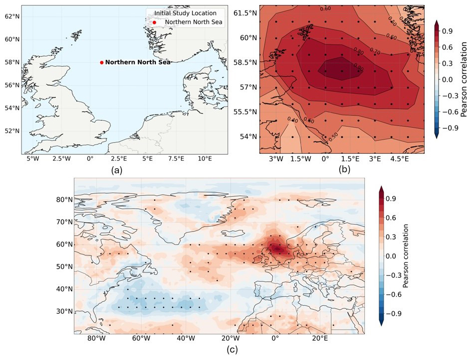
Figure 1 (a) Map of the selected grid cell in the North Sea (1° E, 58° N); (b) correlation between January storm counts (1940–2024) at each North Sea grid point and the storm count time series at the reference location (1° E, 58° N: Northern North Sea); (c) same as panel (b), but extended to all grid cells in the North Atlantic. In panels (b) and (c), we calculated the statistical significance using a Monte Carlo permutation test (100 iterations). Correlations exceeding the 95 % confidence level (p < 0.05) were identified as statistically significant and marked with black dots.

As the correlations shown in Fig. 1a become somewhat smaller towards the coasts of the North Sea, we also examined two additional grid cells near the coast to analyse the impact of stratospheric temperature and zonal wind anomalies on other areas of the North Sea. We added two more grid cells located at the UK and German coasts because these areas are near land, where the greatest societal and economic impacts occur. As for the UK coast, we chose the grid cell near Hull, a port city in East Yorkshire, England (8° E, 54° N). The second grid is chosen along the German coast, near Bremerhaven (1° E, 54° N) (Fig. 2).

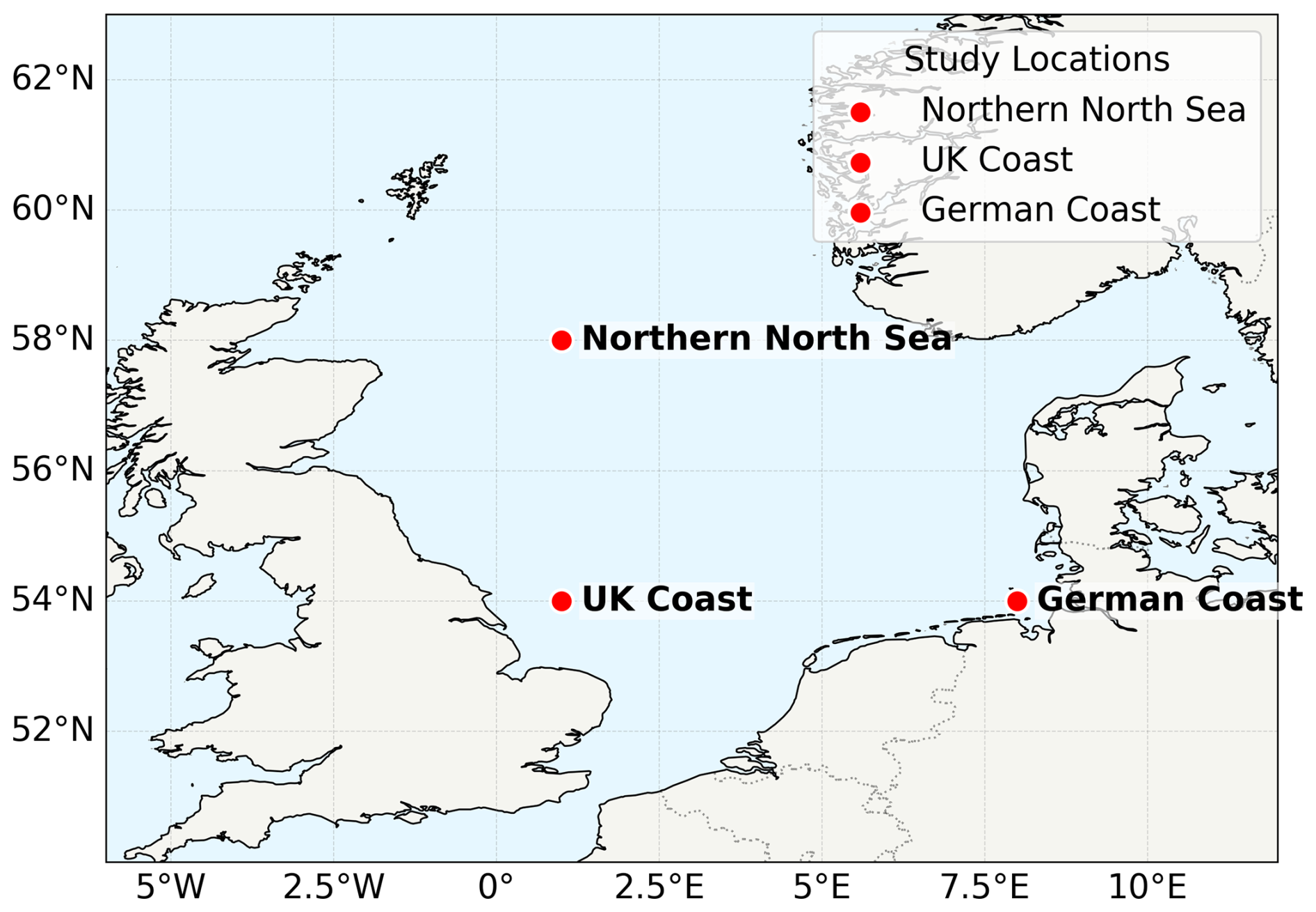
Figure 2 Location of the selected North Sea grid cells used in this study. The central grid cell (Northern North Sea) represents basin-wide storminess, while additional grid cells near the UK and German coasts are used for supplementary analyses.

Throughout the paper, we used Pearson's correlation instead of the Martingale difference or Spearman's correlation, despite the discrete nature of the storm count dataset. As we use correlation analysis only for illustrative purposes to show a rough link to the number of storms in January, we chose Pearson’s correlation because it is widely used and readily interpretable.

3 Preliminary considerations on possible predictors: spatiotemporal persistence of storm frequency

The first preliminary question we explored was how persistent the stormy character of a particular month is over time (e.g., whether a stormy January tends to be followed by a stormy February or preceded by a stormy December). Another related question is the spatial coherence of storminess. Figure 1b indicates that our chosen grid cells are largely representative of the North Sea, but it would be helpful to know how large the area of coherence is. These questions can provide information on potential large-scale predictors of storminess. It turns out that the temporal persistence of the monthly number of stormy days is very low. The cross-correlations between the number of stormy days in the winter months, belonging to the same winter season, in the selected North Sea grid cell are shown in Table 1. Similarly, the correlation map (Fig. 1c) between the number of January stormy days in the North Sea grid cell and all other grid cells in the North Atlantic region shows that the coherence length is rather short, with high correlations located only in the region close to the chosen grid cell.

Table 1 Pearson correlation matrix of monthly storm counts (December–March) at the reference North Sea grid point. Correlations are computed between annual storm-count time series for each winter month over the analysis period (1940–2024). None of these values are statistically significant.

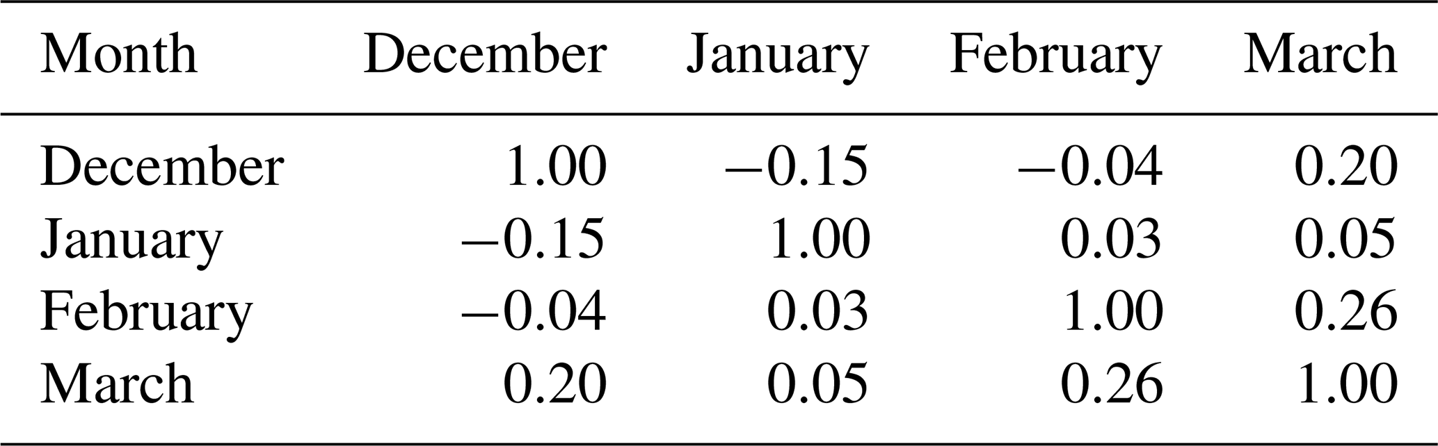
This short spatio-temporal coherence is, on average, incompatible with a relevant role for large-scale SST patterns, since SST anomalies persist for several months (Kushnir, 1994). If SSTs were a relevant predictor of North Sea storminess, a stormy January would tend to be preceded by a stormy December and followed by a stormy February. This is not what we observe.

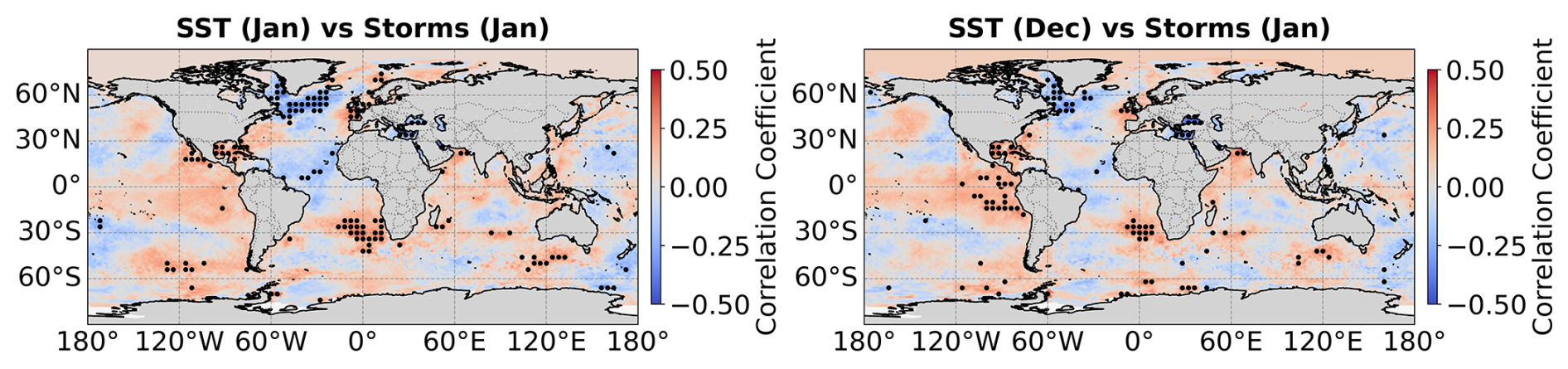
Figure 3 Global correlation maps between sea surface temperature (SST) and North Sea storminess for two cases: simultaneous January–January and 1-month lagged December–January. Statistical significance was assessed using a Monte Carlo permutation test (100 iterations). Correlations exceeding the 95 % confidence level (p < 0.05) are considered statistically significant and are indicated by black dots.

By a similar reasoning, large-scale patterns of remote SST anomalies, e.g., in the Tropical Pacific or the North Atlantic, would plausibly drive storminess over large areas in Europe and perhaps beyond the North Atlantic. The possible mechanisms for atmospheric wave trains excited by SST anomalies would modulate storminess at continental scales, not just in the North Sea. We also examined the correlation between global SST and storminess in the North Sea across two scenarios: January–January and December–January (Fig. 3). The calculated Pearson correlations are very low in all cases. A weak signal emerges in the Eastern Pacific and in the North Atlantic south of Greenland. The Tropical Pacific signal is reminiscent of an El Niño pattern, indicating that warmer SSTs in this area in December and January are weakly linked to the North Sea storminess in January. The correlations are low. Though the sign does not match previous findings, which instead link La Niña patterns to a stronger polar vortex (and thus potentially with increased storminess at the surface). These arguments suggest that large-scale SST patterns are not a reliable predictor of storminess in the North Sea for the following month on average, although they may play a role in individual extreme years. Also, cold SSTs in the North Atlantic during December and January seem to be linked to January North Sea storminess. Again, the correlations are low, and the physical impact of North Atlantic SSTs on the atmospheric circulation at short seasonal timescales is by no means established, even after rather intensive research over the last two decades (see, for instance, Tao et al., 2023 and the references in its introduction).

For these reasons, we turned our attention to shorter-lived atmospheric precursors of storminess. Among those, lower stratospheric temperatures and the occurrence of SSWs have been suggested as drivers of perturbed atmospheric dynamics in this region (Domeisen, 2019; Baldwin et al., 2021). However, the relatively small-scale coherence of storminess suggests that storminess in the North Sea would be driven by particular, likely also regionally constrained, configurations of SSWs (specifically vortex displacement vs. vortex split events) and lower-stratospheric winds, rather than solely by circumpolar dynamics of the polar vortex. Our hypothesis is therefore that the state of the circumpolar polar vortex may be a precondition for storminess in the North Sea, but that this preconditioning would need to be further modulated by regional dynamics that affect the North Sea rather than other adjacent regions. Such modulation may arise from intraseasonal modes of variability, for example, the Madden–Julian Oscillation (MJO), which has been shown to influence the North Atlantic circulation through both tropospheric and stratospheric pathways, including impacts on the polar vortex and the NAO (Yadav et al., 2024). However, while the MJO can provide an important source of variability in the large-scale background state, its influence alone appears insufficient to provide a general predictability of North Sea storminess (Fig. 3), suggesting that the North Sea surface response depends on the combined state of the stratosphere and regionally specific atmospheric dynamics.

3.1 Precursors of stormy Januaries

To identify the configuration of the precursors, stratospheric temperature, and stratospheric winds that lead to stormier Januaries in the North Sea, we selected the five stormiest Januaries and the five calmest (no storm) Januaries within the study period. For each case, we calculated the average air temperature and zonal and meridional wind anomalies (deviations from the climatological December mean) at 70 hPa in December, using daily ERA5 data. This allowed us to examine how the stratospheric state in December varies with the storminess of the following January.

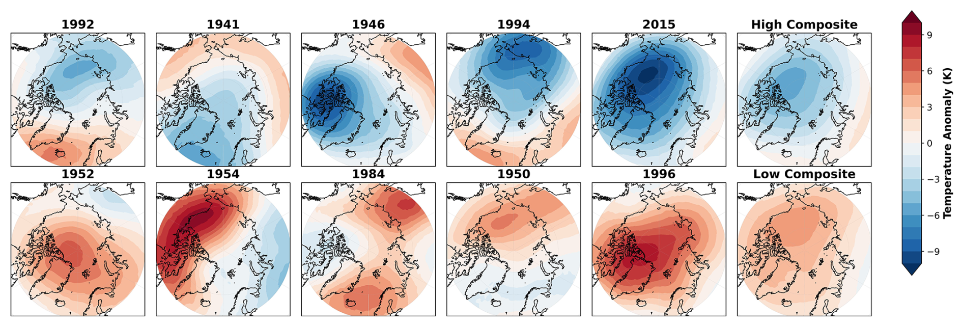
Figure 4 Air temperature anomalies at 70 hPa in the Decembers preceding Januaries characterised by a high (upper row) and zero (lower row) number of stormy days in the Northern North Sea grid cell.

The results show that the stratospheric air temperature tends to be significantly colder already in the Decembers preceding stormier Januaries (Fig. 4). This supports previous studies suggesting that stratospheric air temperature anomalies are key precursors of winter storm activity (Krieger et al., 2024). Figure 4 further shows that the stormiest Januaries (top row) are generally preceded by colder stratospheric conditions in December, whereas Januaries with no storm activity (bottom row) are associated with comparatively warmer stratospheric temperatures in the preceding month.

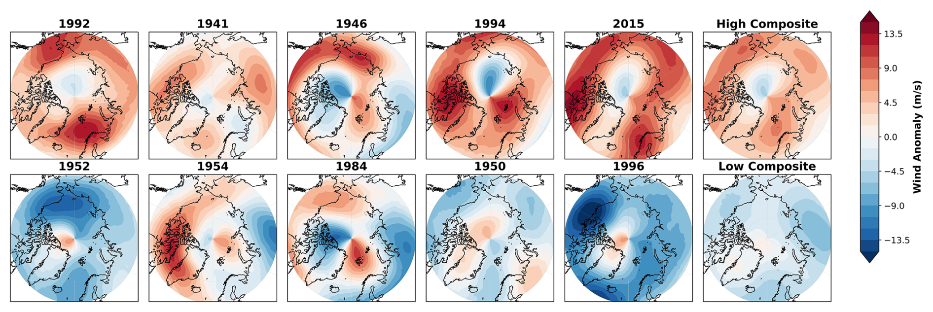
Figure 5 Zonal wind anomalies at 70 hPa in the Decembers preceding Januaries characterised by a high (upper row) and zero (lower row) number of stormy days in the Northern North Sea grid cell.

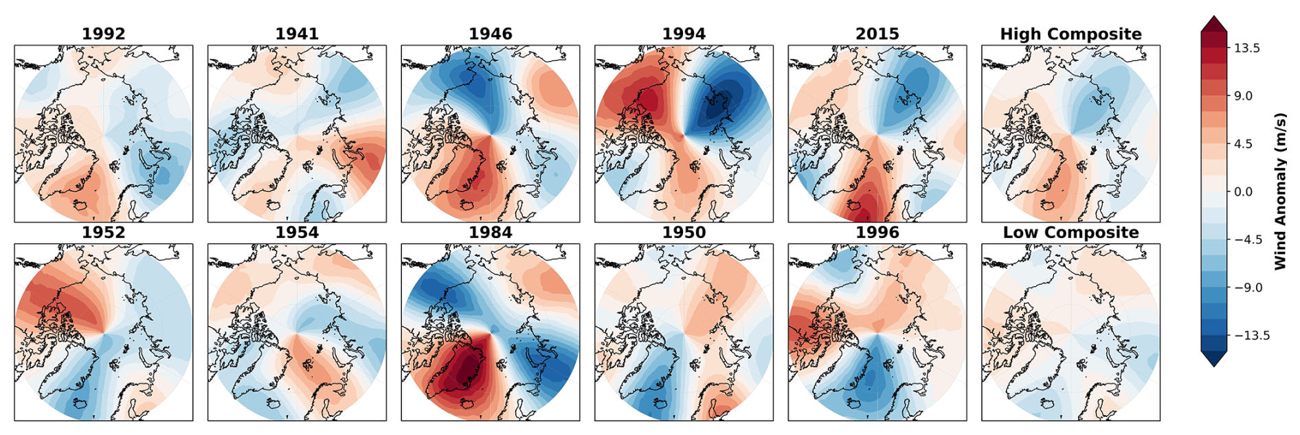
Figure 6 Meridional wind anomalies at 70 hPa in the Decembers preceding Januaries characterised by a high (upper row) and zero (lower row) number of stormy days in the Northern North Sea grid cell.

A similar analysis was performed for the anomalies of the stratospheric zonal and meridional wind components at 70 hPa. Specifically, we computed the corresponding anomalies for the Decembers preceding the Januaries with the five highest and five lowest storminess values. We found that monthly mean zonal wind speeds in the stratosphere are stronger during the Decembers preceding stormier Januaries (Figs. 5, 6), consistent with enhanced stratospheric westerlies and a stronger polar vortex. In contrast, the meridional wind anomalies show a weaker and less distinct difference between stormy and non-stormy Januaries (Fig. 6). Nevertheless, a consistent feature across most stormy cases is the presence of positive meridional wind anomalies over the North Atlantic–Barents Sea sector, indicative of anomalous southerly flow. This pattern may favour a more cyclonic circulation over northern Europe and Scandinavia, but its influence appears less robust than that of the zonal wind anomalies.

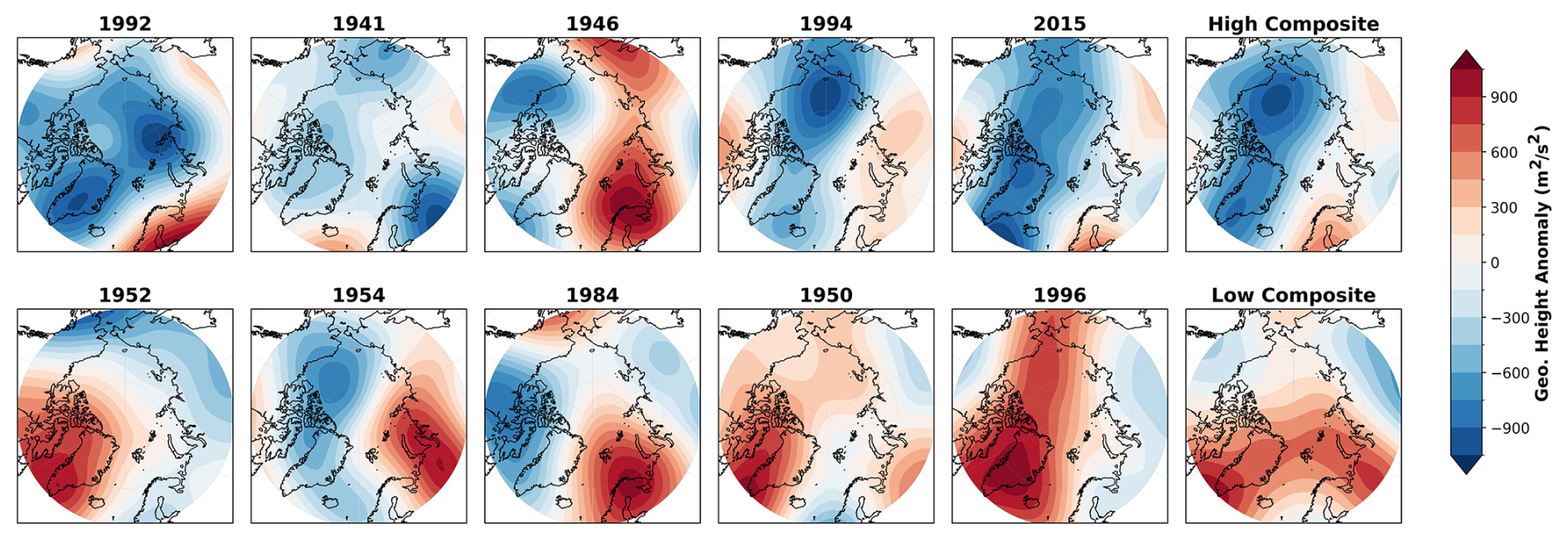
Figure 7 Geopotential height anomalies at 200 hPa in the Decembers preceding Januaries characterised by a high (upper row) and zero (lower row) number of stormy days in the Northern North Sea grid cell.

A similar composite analysis was done for geopotential height anomalies at 200 hPa during the Decembers preceding the five stormiest and five calmest Januaries. The results show a clear contrast between the two groups (Fig. 7). The stormiest Januaries are generally preceded by negative geopotential height anomalies over the Arctic and northern North Atlantic, whereas the calmest Januaries are associated with positive anomalies in the same regions. That means that the stormy Januaries are preceded by lower-than-normal geopotential heights, indicative of a stronger polar vortex and enhanced large-scale circulation. In contrast, calm Januaries are associated with higher geopotential heights, suggesting a weaker polar vortex and more blocked circulation patterns. These results indicate that upper-tropospheric circulation anomalies in December may serve as a useful precursor to January storm activity in the North Sea.

We conducted similar analyses as for the initial North Sea grid cell in the additional grid cells (UK and German coasts in Fig. 2), where stratospheric temperature, wind speed and geopotential height anomalies were examined (Figs. A1, A2, A3, A4, A5, A6, A7, A8 in the Appendix). These coastal locations show behaviour consistent with that of the Northern North Sea grid cell, thereby supporting the robustness of the identified anomaly patterns and the main conclusions of this study.

These identified patterns of average anomalies in the Decembers preceding Januaries with the highest frequency of North Sea stormy days were used to modify the initial conditions in simulations with the atmospheric emulator ACE2, starting on 1 December and running for 2 months. The output was then compared with corresponding years, starting with observed initial conditions on 1 December. The results are described in the next sections.

A similar procedure was applied to the other two winter months, December and February, but, as discussed later, the signal and predictability were weaker than in January.

3.2 ACE2: ML-based atmospheric model

We used the ACE2 (AI2 Climate Emulator, version 2) model to emulate atmospheric variability over the last 80 years. ACE2 is an autoregressive machine learning model that simulates atmospheric dynamics over timescales ranging from days to decades. It has around 450 million parameters and runs with a 6 h time step, 1° horizontal resolution, and eight terrain-following vertical layers. It is trained to predict two 6 h steps ahead and uses a Spherical Fourier Neural Operator (SFNO), which is designed for data defined on a sphere. It requires prescribed 6-hourly fields of external forcings for surface temperature, top-of-atmosphere solar insolation, and CO₂ concentrations. An important feature of ACE2 is that it conserves global dry air mass and moisture exactly, allowing it to run stably for very long periods, up to thousands of years, without developing artificial drift (Watt-Meyer et al., 2025).

Compared with the first ACE version, ACE2 offers three significant improvements: it includes CO₂ as a forcing, reproduces historical trends over the past 80 years, and applies physical corrections during inference to preserve conservation laws. The model outputs standard meteorological fields: winds, temperature, humidity at 8 atmospheric levels; precipitation; near-surface temperature; surface pressure; and radiative fluxes at the surface. During training, some diagnostic variables are weighted differently based on their behaviour, and additional corrections help ensure that precipitation and evaporation remain consistent with changes in atmospheric moisture.

The ACE2 version used here was previously trained by its authors on ERA5 data (Watt-Meyer et al., 2025) (a previous version was trained on the output of the global atmospheric model SHiELD; Watt-Meyer et al., 2023). It can generate realistic features, such as the Madden-Julian Oscillation and tropical cyclones, the ENSO cycle, and capture long-term trends. Despite being a machine-learning model, ACE2 can produce stable, physically meaningful climate simulations at a much lower computational cost than traditional climate models (Watt-Meyer et al., 2025).

In a typical simulation with the ACE2 model, the model is initialised with a snapshot of initial conditions and fields of external forcings covering the simulation period. Here, we will use the ACE2 model to conduct two sets of simulations. Within each set, each simulation covers selected 2-month periods, starting on 1 December and ending on 31 January. The initial conditions for one set are taken from the ERA5 reanalysis. In the second set, the initial conditions on 1 December are perturbed using modified fields of air temperature and the two wind components at 70 hPa.

Although the maps shown in Figs. 4, 5, and 6 suggest that the main signal for storminess is found in the temperature and zonal wind fields, we also included the meridional wind for a closer physical consistency with geostrophy. In these initial simulation steps, there will be a physical inconsistency between these fields at 70 hPa and the other model stratospheric layers, but we assumed that this inconsistency would rapidly disappear.

Note that the temporal evolution of the unperturbed set will rapidly diverge, after a few days, from the observed evolution encapsulated in ERA5, since the ACE2 model is not run with any data assimilation. In this sense, it mimics an initialised free-running weather prediction model with prescribed boundary conditions. However, using these simulations, we explore whether perturbed initial conditions can still drive the ACE2 model to produce stronger or weaker winds in the North Sea region several weeks after initialisation.

We used ACE2 because it provides a tool for simulating atmospheric variability at high temporal resolution while remaining computationally very efficient. Our focus was on understanding stratospheric forcing of the troposphere, primarily through stratospheric air temperature anomalies, and ACE2 enabled quick, flexible emulation of these dynamics. We were able to generate simulations efficiently and repeatedly, which was critical for testing different configurations and initial conditions.

ACE2: Preprocessing

We start this subsection by explaining how the ACE2 initial conditions were prepared. The initial states provided by the ACE2 package (Ai2, 2025) stem from ERA5, and we selected December months for which the following January was relatively calm (one to two storms). We ran ACE2 for multiple Decembers associated with low January storminess, each with distinct initial conditions, and present six representative cases. These years were selected because their subsequent Januaries showed relatively low storm activity in ERA5 (one to two storms), allowing the influence of the altered initial conditions to stand out more clearly. The initial condition is set for 1 December, and the model is then run for 60 d. For each case, we first run the model starting on 1 December, 00:00 UTC using the unmodified initial condition (the “control” run). Then we rerun it with modified initial conditions (the “perturbed” run). We conducted this pair of runs for each of the six selected cases. By comparing these pairs of runs, we can see whether the changes we introduce in the stratosphere lead to stronger surface winds.

Next, we describe how the initial conditions were modified. The anomaly maps of air temperature and zonal and meridional wind shown in Figs. 4, 5, and 6 reveal clear stratospheric circulation patterns. Based on these patterns, we focus on monthly mean anomalies from December 2015, as Fig. 4 shows a relatively cool polar stratosphere at that time. Such conditions are commonly associated with a positive NAO–like circulation and enhanced winter storm activity (Domeisen, 2019; Domeisen and Butler, 2020; Charlton-Perez et al., 2018). The air temperature and wind fields at 70 hPa are used to construct the “polar mask”. This mask is then added to the corresponding variables in the unperturbed ACE2 initial conditions to impose a modified stratospheric state. The model is subsequently rerun for 2 months, and the resulting changes in the simulated atmospheric evolution are analysed.

3.3 Random Forest Regression model

To support the results obtained with the ACE2 model, we use another established ML method, namely Random Forest Regression (RFR), to establish a data-driven month-to-month predictive scheme that takes as input the monthly means of stratospheric fields of 70 hPa air temperature and winds to produce a forecast of the number of stormy days in the following month. RFR is an ensemble learning method that combines many decision trees to produce a single prediction. Each tree is trained on a random subset of the data and a random subset of the predictors, reducing the influence of noise and improving the stability of the final estimate. The method was introduced by Breiman (2001) and has since become widely used in climate science because it can recover complex, nonlinear relationships without requiring strong assumptions about the data structure. It also handles large predictor sets, spatial correlations, and predictor interactions well, which is especially relevant for atmospheric fields (Gagne et al., 2019).

In this study, we used RFR to examine how the state of the stratosphere within the polar region in December relates to storminess in the North Sea the following January (the December–January relationship). We then applied the same approach to other month pairs (October–November, November–December, January–February, and February–March) to examine how this relationship evolves across the season. The predictors consist of monthly mean fields of air temperature at 70 hPa, zonal wind at 70 hPa, and geopotential height at 200 hPa from the ERA5 reanalysis spanning from 1940 to 2024, within the polar region (60 to 90° N). For each year, the gridded fields were flattened into feature vectors, so each December became a single sample representing the spatial pattern of the stratosphere. The predictand is the number of stormy days observed in our selected North Sea grid cell during the following January.

RFR: Preprocessing

To construct the dataset used for predicting January storminess in the North Sea, we first derived a storm index from ERA5 daily 10 m wind data. The total number of such days per January forms the annual storm index used as the predictand.

Three dynamical and thermodynamical predictor fields from ERA5 were used: air temperature at 70 hPa, geopotential height at 200 hPa, and zonal wind at 70 hPa. Each dataset was converted to a −180 to 180° longitude system, sorted, and spatially restricted to the Arctic domain (60 to 90° N). The latitude and longitude dimensions were then flattened so that each December map becomes a single one-dimensional feature vector.

Finally, all predictor fields were temporally aligned with the storm index. The resulting arrays were stored in a compressed archive to ensure reproducibility. For the machine-learning experiments, the available years were randomly divided into a training set (70 %) and an independent test set (30 %). The same random split was used for all experiments to ensure consistency across different predictor configurations. No cross-validation was applied. Predictor fields were standardised using a StandardScaler, concatenated, and reduced in dimensionality using Principal Component Analysis (PCA) prior to training the Random Forest models.

4 Results

4.1 ACE2 Model output

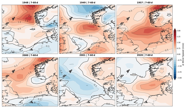
We ran ACE2 for multiple Decembers associated with relatively low January storminess, each with distinct initial conditions, and present six representative cases. Figure 8 illustrates the results for the simulations started on 1 December 1948, 1949, 1957, 2000, 2001, and 2020. We run the model for 60 d and calculate the difference in mean wind speed (perturbed run − control run) response from 7 December to 31 January (Fig. 8). Over several years, including 1948, 1949, 1957, 2000, and 2020, we observe an increase in surface wind of 0.5–3 m s⁻¹ following the introduction of the stratospheric perturbation.

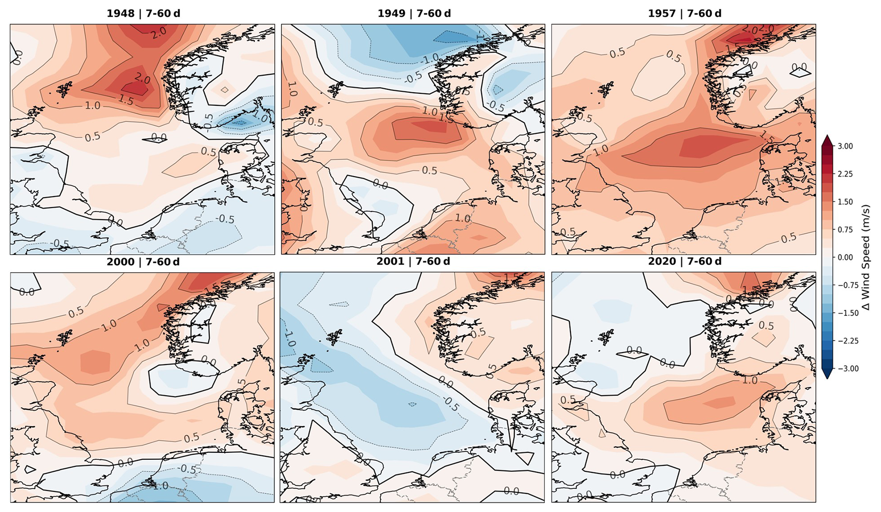
Figure 8 Temporal mean of 10 m wind speed response from ACE2 simulation (perturbed − controlled) for days 7–60 following initialisation. Shown are the difference fields for the cases of December 1948, 1949, 1957, 2000, 2001, and 2020. Warm colours indicate stronger near-surface winds in the perturbed run, while cool colours show reduced winds. For reference, the number of storms in the following Januarys was 1, 2, 1, 2, 1, and 2, respectively.

Although these years, such as 1948, 1949, 1957, 2000, and 2020, were followed by relatively low stormy Januaries in the observations, their responses to the perturbation differ. Therefore, we also present an example of a slightly different situation for the simulation started in December 2001 (Fig. 8). After adding the “polar mask” to the initial condition and running the model for 2 months, surface wind speeds do not seem to increase across the entire region. Rather, we see only a modest increase, mainly south of Norway in the North Sea, but, more broadly, a decrease of 0.5 to almost 1 m s⁻¹. This is not entirely surprising, since it is unlikely that a single factor can explain 100 % of the variability, and we also wanted to show a case where it does not work. In this case, despite an SSW in late December 2001 (Butler, 2023), adding the polar mask to the initial condition and integrating the model for 2 months does not increase surface wind speeds across the entire region. This winter illustrates that stratospheric temperature anomalies alone may not be a sufficient predictor of subsequent North Sea storminess in all cases. During winter 2001–2002, tropical forcing associated with a prolonged Madden–Julian Oscillation (MJO) episode (Yadav et al., 2024) could have contributed to a noticeable whiplash of the NAO, which turned from clearly negative in December 2001 to strongly positive in the ensuing January and February (Henderson et al., 2016), potentially counteracting the expected post-SSW circulation response. Our interpretation is that the SSW and the MJO may have had opposing effects that winter, resulting in an unremarkable number of storms in January 2002, despite the rather strong NAO index during those initial 2 months of 2002. Although this shift in reasoning requires further research, it suggests that exceptionally strong or persistent SST patterns could affect North Sea storminess.

We also performed similar sensitivity experiments initialised in early November. However, no meaningful response was found in the following month (Fig. A9).

Changes in the frequency of extreme wind events

While Fig. 8 shows the obvious increase in wind speed in most cases, we assessed the impact of a strengthened stratospheric polar vortex on surface winds. We analysed the full probability density function (PDF) of daily wind speeds over the North Sea for days 7–60. The analysis considers multiple grid cells across the North Sea region (Longitude: 4° W to 10° E, Latitude: 51 to 61° N), increasing the sample size and improving statistical robustness.

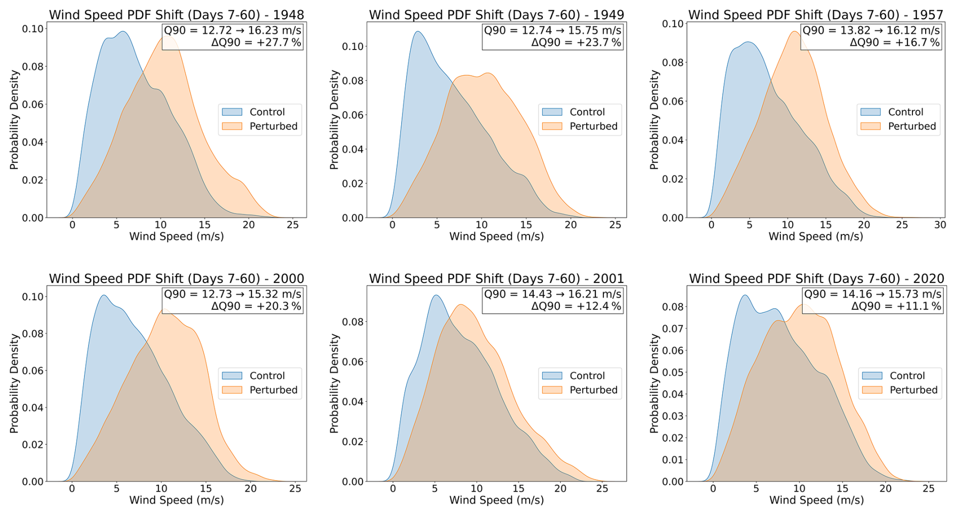
Figure 9 PDFs of daily wind speed over the North Sea (days 7–60) for control and perturbed simulations, aggregated across multiple grid cells (Longitude: 4° W to 10° E, Latitude: 51 to 61° N). The perturbed experiment consistently shows a rightward shift and a more populated upper tail. The figure also includes quantifications of the difference at the 90th percentile of the PDF distributions as a percentage.

Figure 9 shows that, for all selected winters, the perturbed experiment has a clear rightward shift of the wind speed PDF relative to the control. This generally indicates stronger surface winds in January, when the polar vortex is artificially strengthened. The shift is evident across the distribution and is particularly pronounced in the upper tail. The top 10 % of wind speeds show increased probability density in the perturbed simulations, implying a higher likelihood of extreme wind events.

To assess this tail response more clearly, we compared the number of days exceeding the 90th percentile of the control experiment between perturbed and control simulations for days 7–60. Figure 10 presents spatial maps of the resulting percentage point change in the frequency of extreme wind days, computed using the control-based threshold. This approach isolates changes in the upper tail of the distribution and provides a direct measure of extreme event risk.

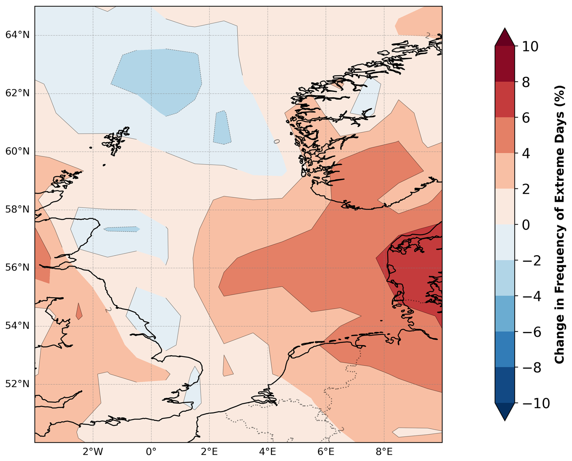
Figure 10 Change (%) in the frequency of wind speeds exceeding the control 90th percentile over the North Sea (days 7–60, all selected years).

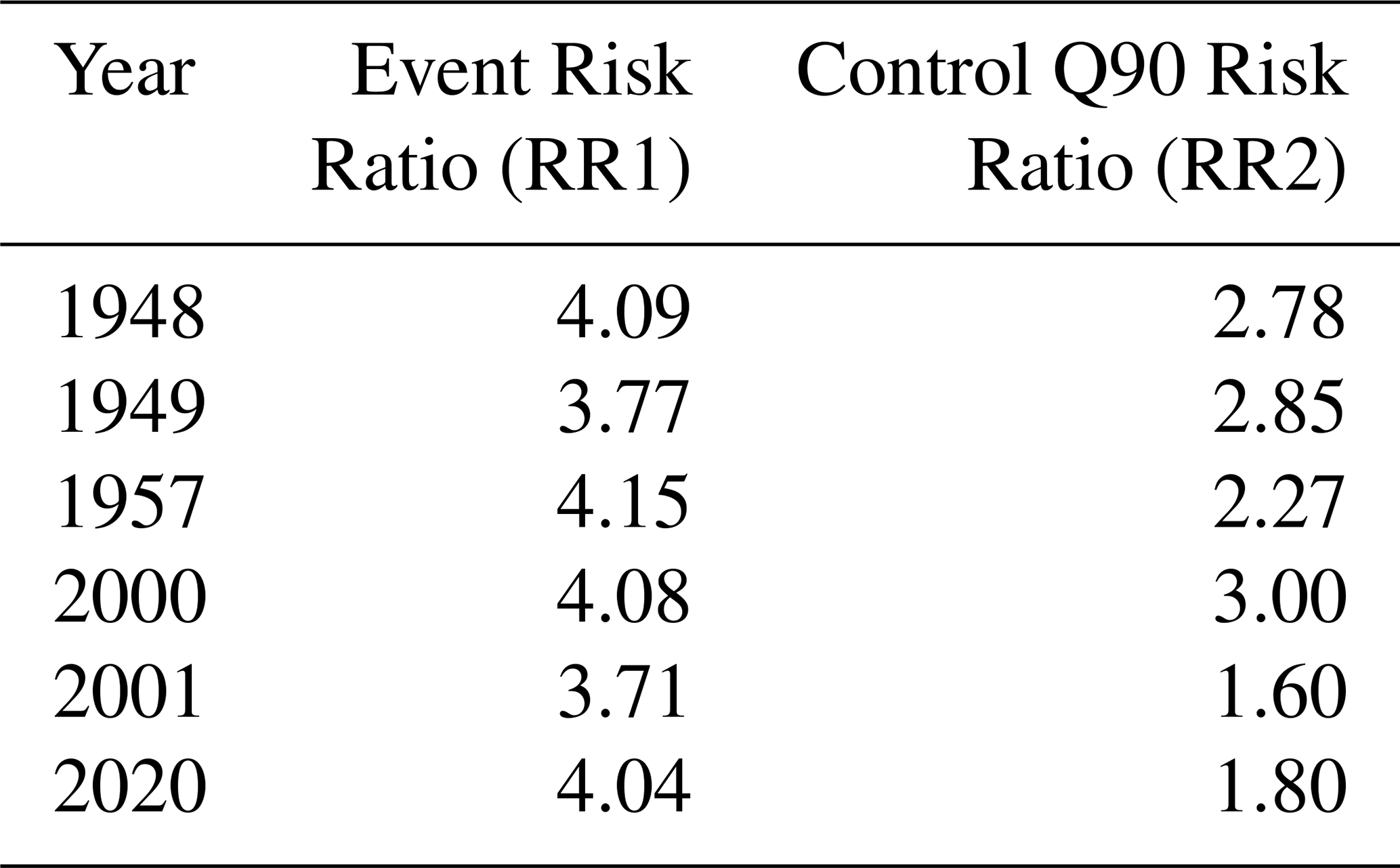
Across most of the North Sea, the frequency of extreme wind days increases in the perturbed simulations. The largest increases, of approximately 2 %–6 %, occur along the coastlines of Denmark, northern Germany, and southern Norway, while parts of the eastern UK coastline show a weak response. Table 2 summarises the changes in the likelihood of 90th percentile wind speed events over the North Sea. Both risk ratio metrics indicate a systematic increase in extreme wind events under a strengthened polar vortex. The Event Risk Ratio (RR1), based on a fixed climatological 90th percentile threshold, ranges from 3.71 to 4.15, indicating that extreme wind speed events become approximately four times more likely in the perturbed simulations. The Control Q90 Risk Ratio (RR2), computed using the 90th percentile threshold derived from each control simulation, ranges from 1.60 to 3.00 and likewise demonstrates a substantial increase in exceedance probability. Together, the PDF and exceedance analyses demonstrate that a strengthened polar vortex leads to both higher wind speeds overall and a systematic increase in the likelihood of extreme surface wind events over the North Sea.

Table 2 Comparison of risk ratios for 90th percentile wind speed events. The first column uses the climatological 90th percentile threshold (Event Risk Ratio), whereas the second column uses the 90th percentile threshold derived from the control simulation (Control Q90 Risk Ratio). The fixed-threshold risk ratio is defined as $\mathrm{RR}\mathrm{1}=P_{\mathrm{pert}}/P_{\mathrm{ctrl}}$, where P_ctrl=0.10 corresponds to the exceedance probability of the control 90th percentile threshold. The control-Q90 risk ratio is calculated as $\mathrm{RR}\mathrm{2}=P_{\mathrm{pert}}(X>\mathrm{Q}{\mathrm{90}}_{\mathrm{ctrl}})/P_{\mathrm{ctrl}}(X>\mathrm{Q}{\mathrm{90}}_{\mathrm{ctrl}})$ (Zhang and Wang, 2019).

4.2 Random Forest Regression model output

The model evaluation shows that the Random Forest captures a meaningful portion of the relationship between December atmospheric conditions and the number of storms observed in the North Sea during the following January (Figs. 11, 12). Across all tested configurations, the best-performing setups yield correlations in the range 0.55–0.60. This indicates that December's large-scale atmospheric conditions account for nearly one-third of the following month's North Sea storminess.

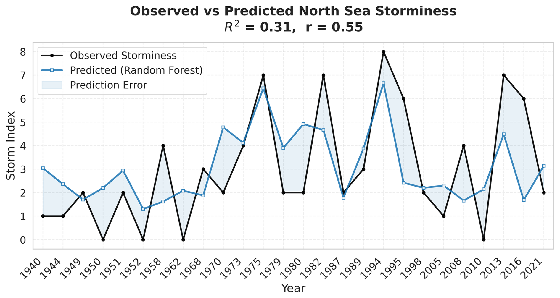
Figure 11 Comparison between observed and Random Forest predicted North Sea storminess (1940–2024). Time series of observed (black-test set) and predicted (blue) storm indices.

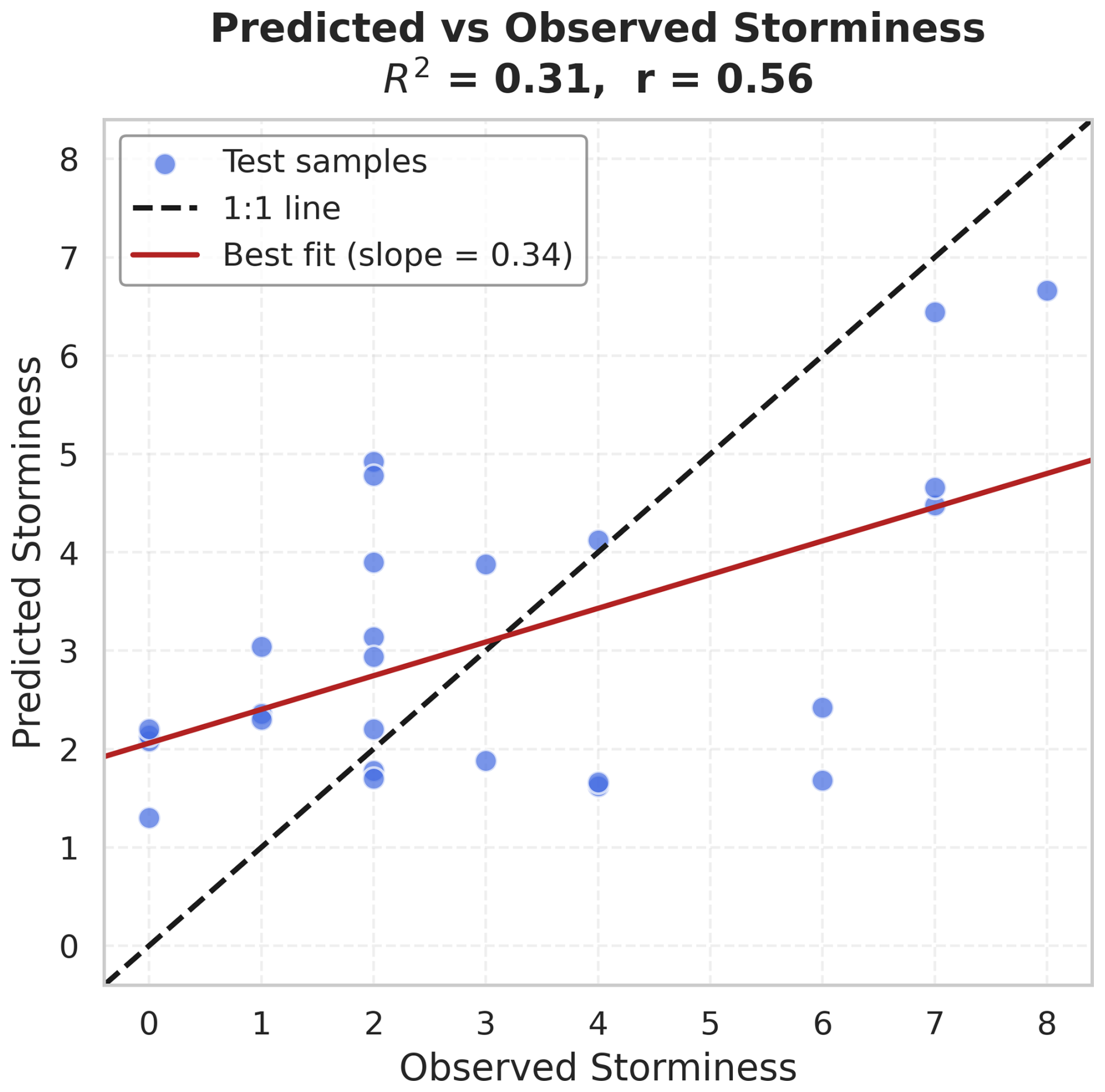
Figure 12 Scatterplot of observed vs. predicted storminess for the same test set as Fig. 11, illustrating model skill.

The scatter plot (Fig. 12) shows the model behaviour on the test set (30 % of the data), which is much smaller and therefore noisier. The correlation of 0.56 and the shallow slope of the red regression line indicate that the model correctly captures the direction of the variability but tends to underestimate and sometimes overestimate extreme values. Nevertheless, the points show that the model rarely fails dramatically; predicted values remain within a consistent band and follow the general trend of the observations. This picture becomes clearer in the time-series comparison (Fig. 11), where observed and predicted storminess evolve in a broadly similar manner. Many peaks and troughs align, particularly in the middle to late part of the test period, indicating that the model reproduces the temporal structure of stormy and calm winters.

Understanding why the model achieves this level of skill requires examining the contributions of the predictors. The feature importance figure (Fig. 13) indicates that PC1 (the first principal component, which captures the dominant pattern of variability in the dataset) and PC5 account for most of the predictive power, followed by PC3, PC2, and several others with smaller but still meaningful contributions.

Figure 13 Importance of Principal Components Used as Predictors in the Random Forest Model.

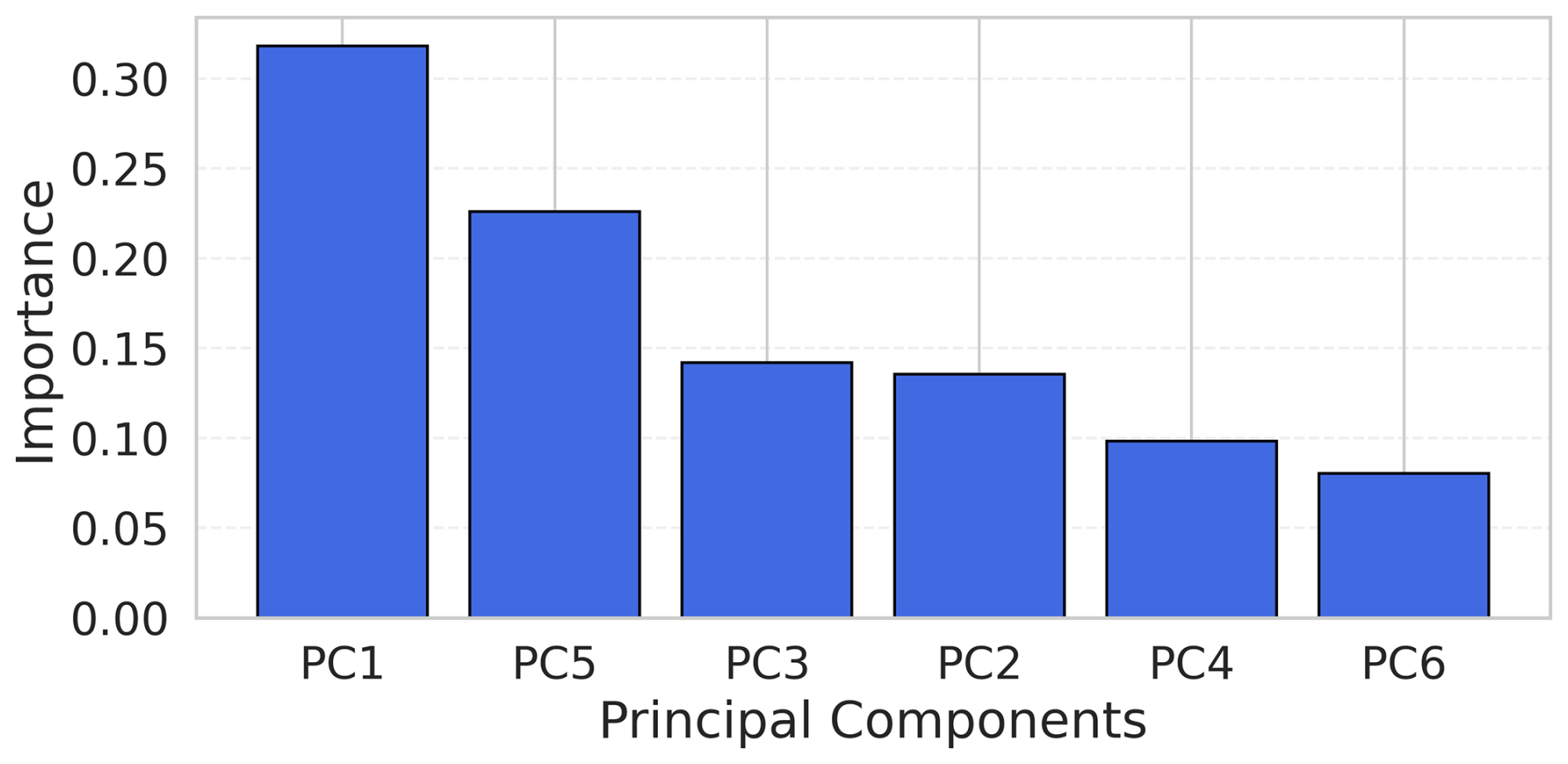
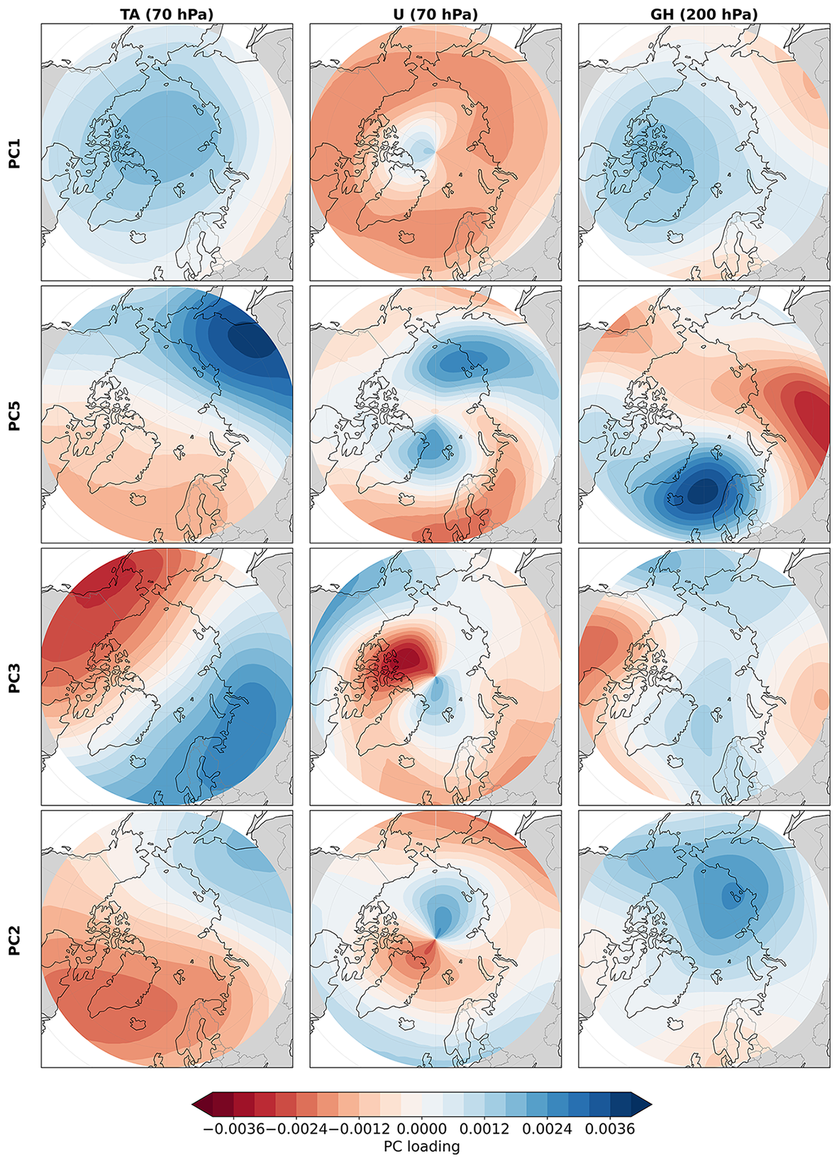
Figure 14 Spatial patterns of the principal component (PC1, PC5, PC3 and PC2) of the December mean fields derived from ERA5 (1940–2024) for air temperature at 70 hPa (TA), zonal wind at 70 hPa (U) and geopotential height at 200 hPa (GH).

To interpret these physically, the PCs' loading maps are essential (Fig. 14). They reveal coherent Arctic-wide structures in temperature at 70 hPa (first column), zonal wind at 70 hPa (middle column) and geopotential height at 200 hPa (third column). A PC loading is the weight that shows how strongly a variable contributes to a principal component. All three fields for PC1 exhibit patterns associated with the polar vortex's strength. The temperature field (first column) at 70 hPa shows positive PC loading across the Arctic, indicating enhanced stratospheric stability, which is also linked to a strong, stable vortex above. The zonal wind pattern (middle column) mirrors this structure, with strong positive westerly anomalies extending across the high latitudes. For geopotential height (third column), PC1 shows a broad region of positive PC loading centred over the polar cap, consistent with an intensified vortex. These three patterns together reflect a dynamically consistent state of the stratosphere in December. PC5, PC3 and PC2, on the other hand, show asymmetric structures that include a distorted polar vortex. According to Zhang et al. (2024), when the polar vortex is weak, the atmosphere becomes less active and less stormy, and weather systems that usually transport air and energy weaken, making it easier for high-pressure systems to form and persist. As a result, more blocking occurs over Greenland, as seen in PC5. This response is typical over northern Europe and the North Atlantic sector; however, this behaviour is not necessarily representative of central and southern Europe. For example, Afargan-Gerstman et al. (2024) showed increased storm activity following sudden stratospheric warming events in these regions using subseasonal reforecast experiments. In such cases, the footprint of the strongest wind speeds tends to occur on the equatorward side of the main storm track, such that regions like Iberia experience an increased risk of surface wind extremes following weak polar vortex or SSW events (Ayarzagüena et al., 2018; Utrabo-Carazo et al., 2024).

Because the polar vortex is a known driver of the North Atlantic circulation in the following weeks, these PC patterns provide a physically meaningful basis for predictability. A strong vortex in December often promotes a stronger, more zonal jet stream in January, increasing the likelihood of frequent storms entering the North Sea region (discussed in Sect. 1). This is precisely the kind of signal the model is taking into account. In short, the predictors primarily represent the large-scale Arctic dynamical environment, particularly the state of the stratosphere and its coupling with the North Atlantic jet.

Predictability within different months

In the previous subsection, we focused only on the predictability of the predictand in January from the predictors in December. Using the same methodological setup as for the December-January pair, we now investigate predictability using the Random Forest approach for different predictor-predictand month pairs, as listed in Table 3.

Table 3 Summary of the Random Forest model performance metrics for different predictor-predictand month pairs. The first month is the predictor month, and the second month is the predictand month. The correlations are calculated between predictions and the target in a reserved independent data set not used for the training of the RF methodology, in a similar fashion to the December–January case. The coefficient of determination is computed as $R^{\mathrm{2}}=\mathrm{1}-\frac{{\sum }_{i=\mathrm{1}}^n{\left(y_i-{\widehat{y}}_i\right)}^{\mathrm{2}}}{{\sum }_{i=\mathrm{1}}^n{\left(y_i-\stackrel{\mathrm{‾}}{y}\right)}^{\mathrm{2}}}$, where y_i are the observed values, ${\widehat{y}}_i$ are the predicted values, and $\stackrel{\mathrm{‾}}{y}$ is the mean of the observations. R²>0 indicates that the model explains a fraction of the variance in the target variable and performs better than a prediction based solely on the mean observation. R²=1 corresponds to a perfect prediction, while R²=0 indicates performance equivalent to using the observed mean as a predictor. R²<1 occurs when the residual sum of squares exceeds the total sum of squares, implying that the model performs worse than the mean-value predictor.

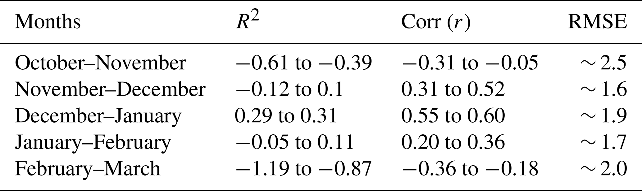
We observe that the correlation reaches negative numbers for October–November and February–March. Evidently, we observe higher correlations during the months of November–December, December–January, and January–February. This can be related to the seasonal cycle of the polar vortex, which forms in autumn (September to November), peaks in winter (December to February), and breaks down in spring (March onwards) (Domeisen and Butler, 2020). We observe that predictability is higher during winter than in autumn or spring. This may be related to stratospheric variability, as the persistence of polar vortex anomalies strengthens in midwinter (Kidston et al., 2015). Although these anomalies can last from January into February, their effects at the surface are stronger later in winter. This suggests that persistence alone is not enough, and effective downward coupling is also needed. Through this coupling, polar vortex anomalies in the lower stratosphere can influence tropospheric circulation. In the Northern Hemisphere (NH), SSWs occur on average every other year and often lead to persistent blocking over Greenland associated with the negative phase of NAO (Charlton-Perez et al., 2018; Domeisen, 2019), altering surface weather for weeks to months (Limpasuvan et al., 2005). A strengthening of the stratospheric polar vortex, on the other hand, tends to exert an opposing downward influence on the NAO, towards its positive phase (Domeisen and Butler, 2020).

5 Limitations and future work

While this study highlights new connections between stratospheric conditions and North Sea storminess, several limitations should be acknowledged. The storminess metric is based solely on surface wind speed and does not include sea-level pressure or precipitation. The ERA5 datasets also have weaknesses: the ERA5 dataset uses a data assimilation scheme to keep its state close to observations; fields such as the surface precipitation rate and radiative fluxes are not constrained and exhibit nontrivial biases relative to satellite and station observations (Hersbach et al., 2020; Urraca et al., 2018). ERA5 is also known to underestimate strong offshore winds relative to station observations (Gandoin and Garza, 2024). This does not affect the proof of concept of the RF or ACE2 methodology, but a more operationally oriented assessment should use ERA5 and station observations as RF training data.

The dynamics of SSWs have been briefly discussed here but not thoroughly investigated, as the primary focus has been on the impact of stratospheric conditions on seasonal predictability. Our results, however, hint at the importance of dynamics with spatial scales smaller than pan-circumpolar to target the predictability of seasons with more frequent extreme winds, which would require a more spatially detailed description of the dynamics of SSWs. A further limitation is that our analysis focuses on signals that are robust across the full record, rather than on the predictability of individual events. Studies have shown clear stratosphere–troposphere linkages in specific late-winter seasons (Williams et al., 2025), but such relationships do not emerge consistently here. This suggests that while ACE2 captures the most recurrent signals, it may miss event-specific predictability that departs from the long-term average, which could be explored in future work using more targeted or conditional approaches. A clear example is the 2001–2002 winter discussed in previous sections.

6 Summary and conclusion

The purpose of this research is to improve the month-to-month storm prediction skill by using different machine learning models. In this work, we develop statistical and machine-learning models to quantify the relationship between large-scale stratospheric conditions in one winter month and observed storminess in the North Sea during the following month.

The study uses techniques such as PCA for dimensionality reduction and Random Forest regression for prediction. The models extract dominant patterns in stratospheric temperature, upper-tropospheric geopotential height, and stratospheric wind anomalies from 1940 to 2024. To test physical attributes, we use the ACE2 climate emulator to conduct controlled experiments by perturbing the initial stratospheric conditions. By adding observed anomalies, such as cold temperature patterns and wind anomalies from December 2015, into different historical years, we can observe their impact on the subsequent month’s surface winds. These experiments allow us to assess whether specific stratospheric states actively contribute to a stormier or calmer North Sea winter, rather than just correlating with it.

The key findings begin with the ACE2 experiments. By imposing the colder stratospheric temperature anomalies and the associated wind patterns observed in December 2015, the simulations were designed to test whether the known link between lower polar stratosphere dynamics and surface weather can be used for a month-to-month prediction scheme: a perturbed stratosphere can intensify surface winds in the following month. The model results generally support this hypothesis: in several cases, surface wind speeds begin to increase after day 7 and continue to strengthen through day 60. However, in one case (2001), no increase in surface wind speed is observed during the 7–60 d period, indicating that the stratospheric state does not solely control enhanced surface winds and that other factors also play a role (Sect. 4.1).

The Random Forest model links December stratospheric and upper-tropospheric atmospheric conditions to January storminess in the North Sea. After preprocessing the ERA5 datasets (air temperature at 70 hPa, geopotential height at 200 hPa, and zonal wind at 70 hPa) and reducing dimensionality with PCA, the model achieves predictive skill, with correlations of 0.55–0.60, and explains roughly one-third of the observed variability. The results show that the first principal component, representing a strong, dynamically coherent Arctic pattern across all three fields, highlights the central role of the polar vortex. PC5, PC3, and PC2, in contrast, display asymmetric spatial patterns indicative of a distorted polar vortex. When extending the analysis to different month pairs (e.g November predictors to predict December storminess), predictability remains moderately high (r = 0.20–0.36) during the core winter months, when the polar vortex is well developed, but drops sharply during autumn and spring, when the vortex is forming or breaking down. This pattern aligns with the known seasonal cycle of the vortex and the period of strongest stratosphere–troposphere coupling.

In conclusion, our findings from ACE2 experiments and RFR models show a moderately robust link between December stratospheric states and January North Sea storminess. Using these methods, we develop a predictive tool that accounts for approximately 30 % of storm variability. These insights represent a significant step toward mitigating the socio-economic risks posed by winter wind extremes in northwestern Europe.

Appendix A

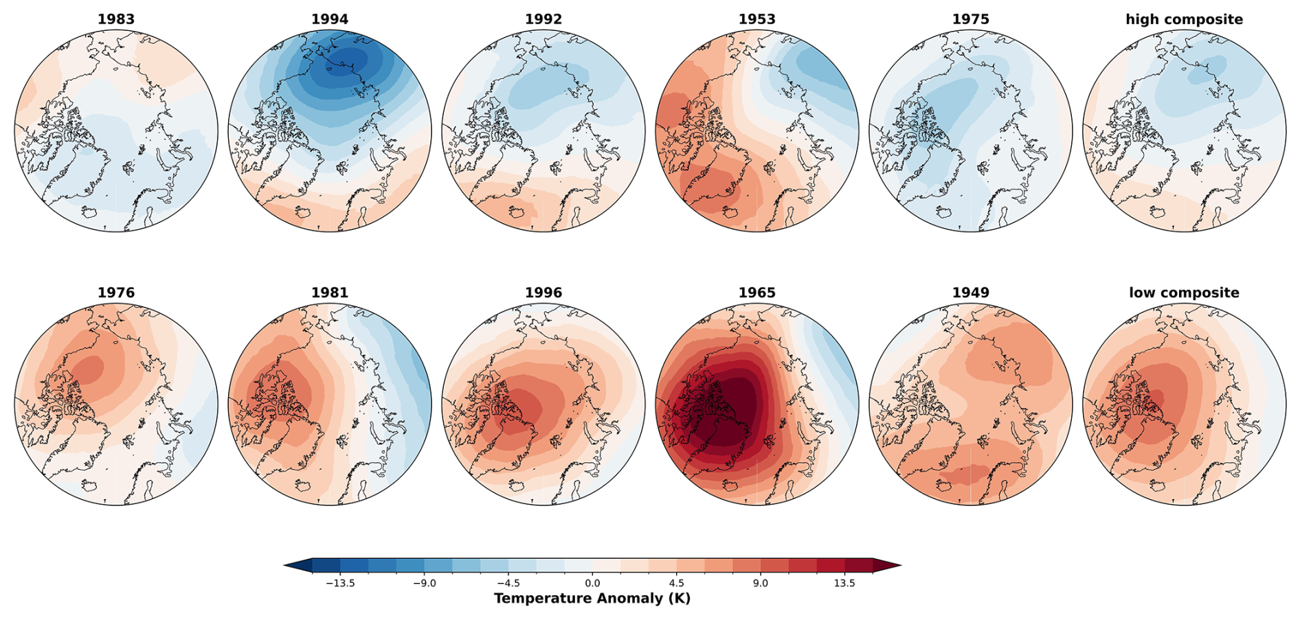
Figure A1 Air temperature anomalies at 70 hPa in the five Decembers preceding the five Januaries with high storm activity (top row) and low storm activity (bottom row) in the North Sea (UK Coast).

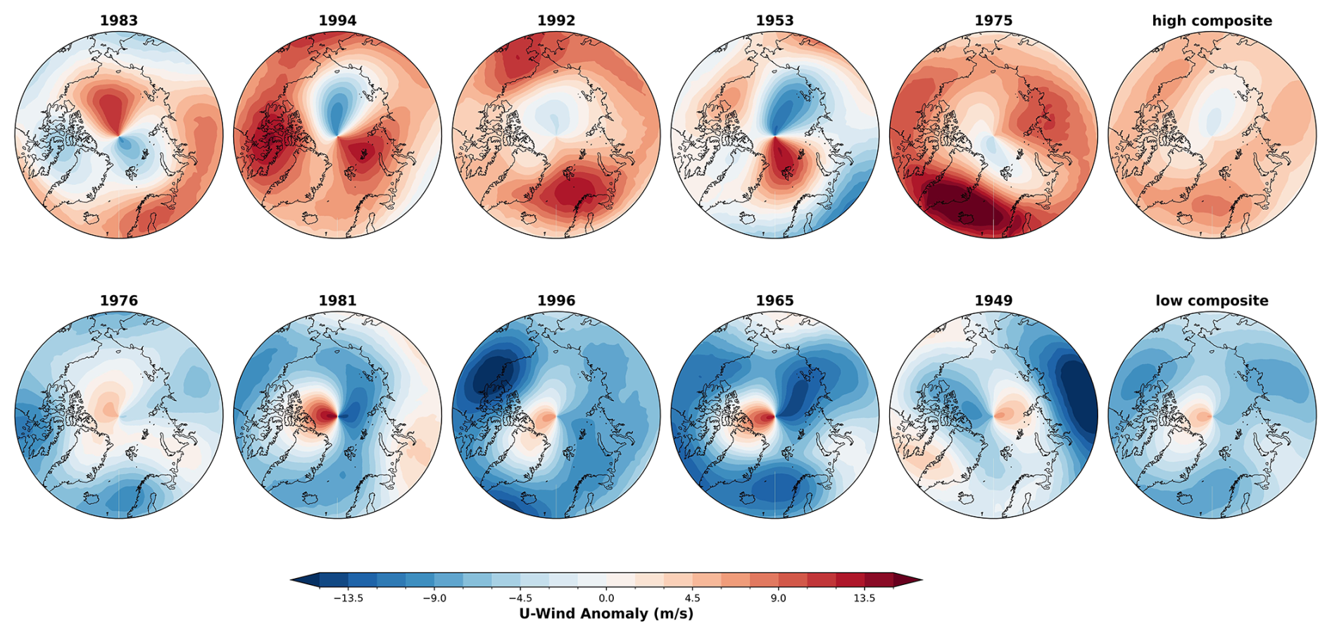
Figure A2 Zonal wind anomalies at 70 hPa in the five Decembers preceding the five Januaries with high storm activity (top row) and low storm activity (bottom row) in the North Sea (UK Coast).

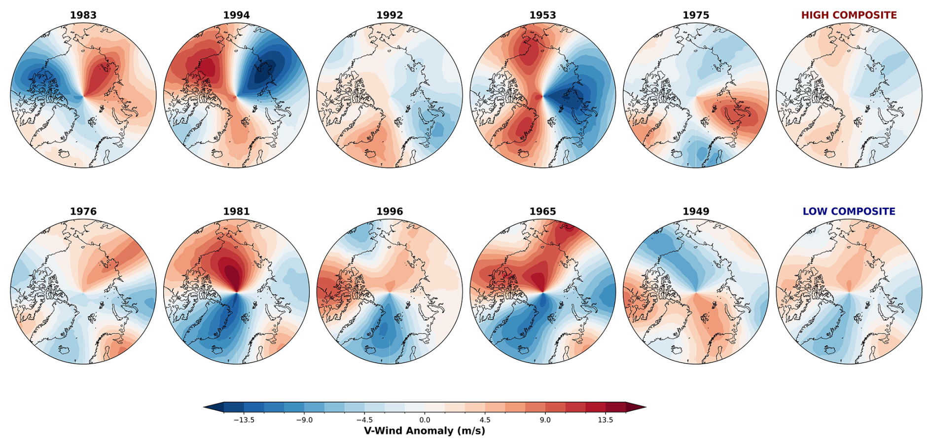
Figure A3 Meridional wind anomalies at 70 hPa in the five Decembers preceding the five Januaries with high storm activity (top row) and low storm activity (bottom row) in the North Sea (UK Coast).

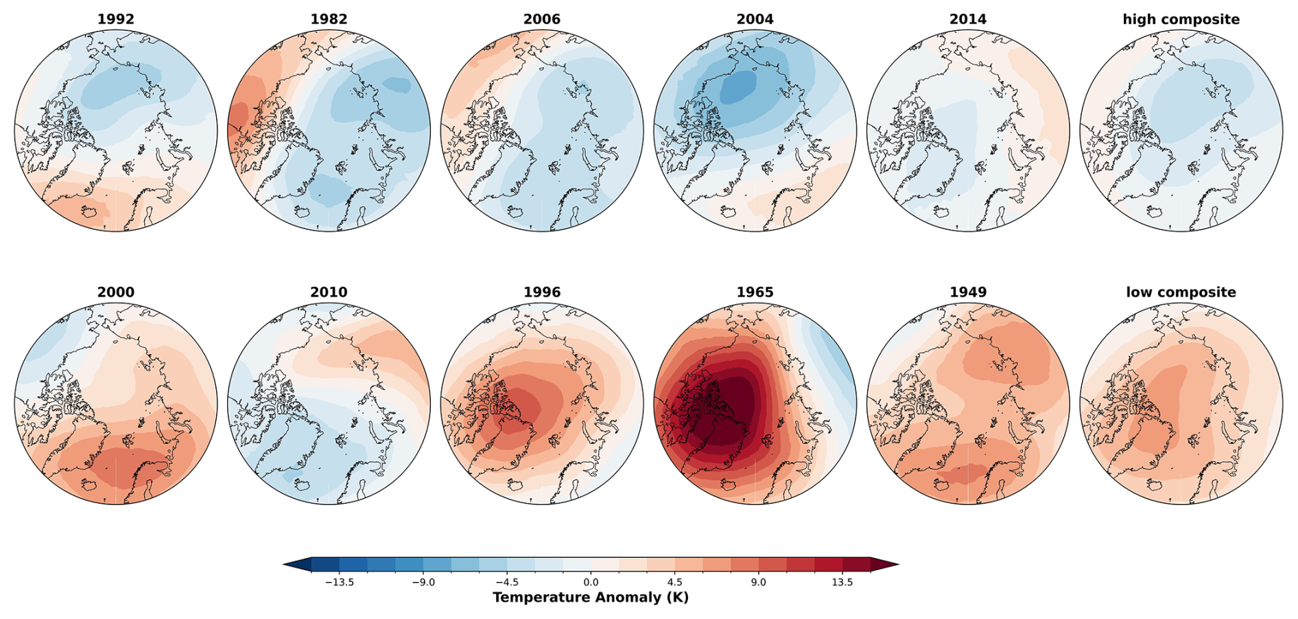
Figure A4 Air temperature anomalies at 70 hPa in the five Decembers preceding the five Januaries with high storm activity (top row) and low storm activity (bottom row) in the North Sea (German Coast).

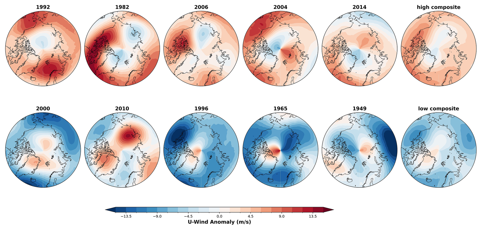
Figure A5 Zonal wind anomalies at 70 hPa in the five Decembers preceding the five Januaries with high storm activity (top row) and low storm activity (bottom row) in the North Sea (German Coast).

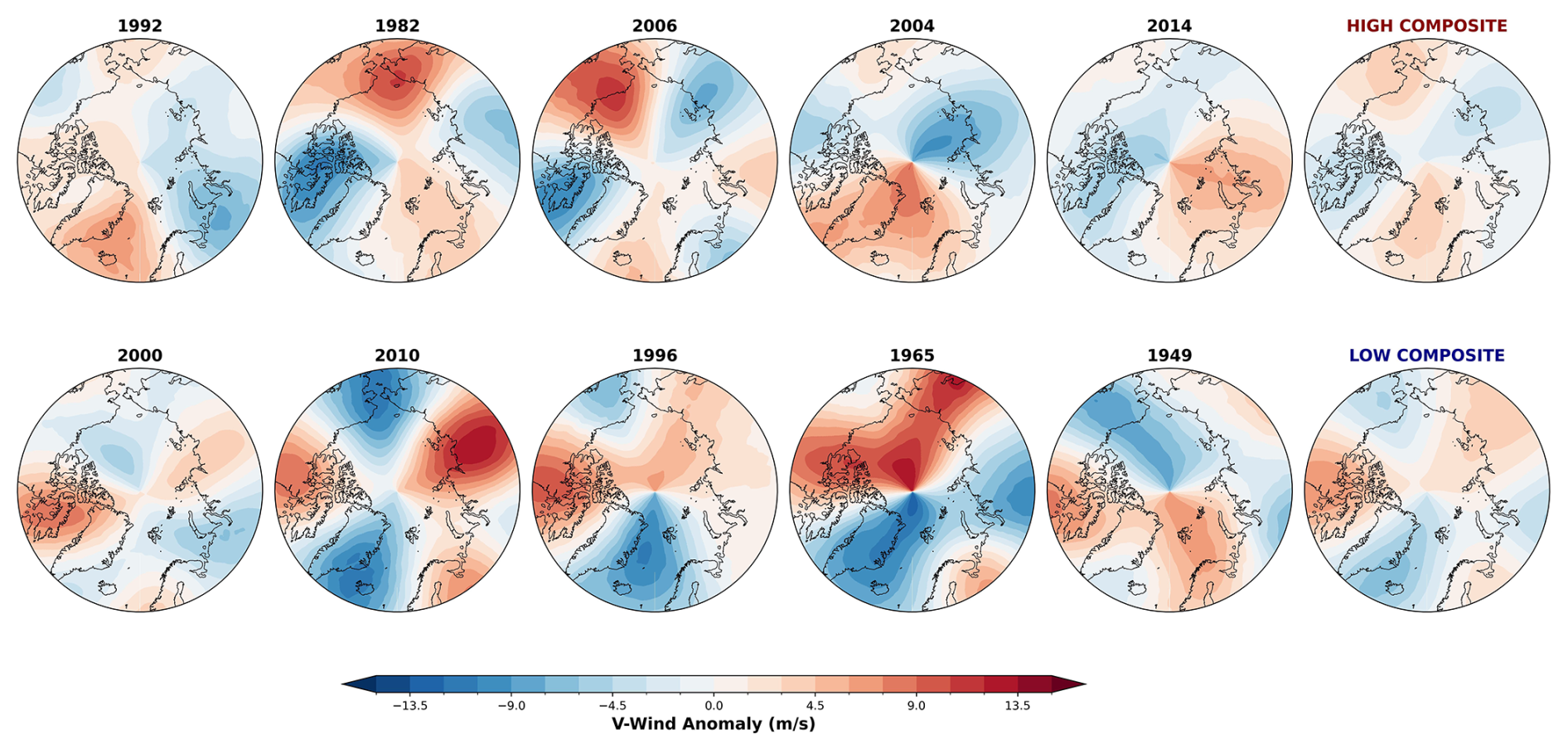
Figure A6 Meridional wind anomalies at 70 hPa in the five Decembers preceding the five Januaries with high storm activity (top row) and low storm activity (bottom row) in the North Sea (German Coast).

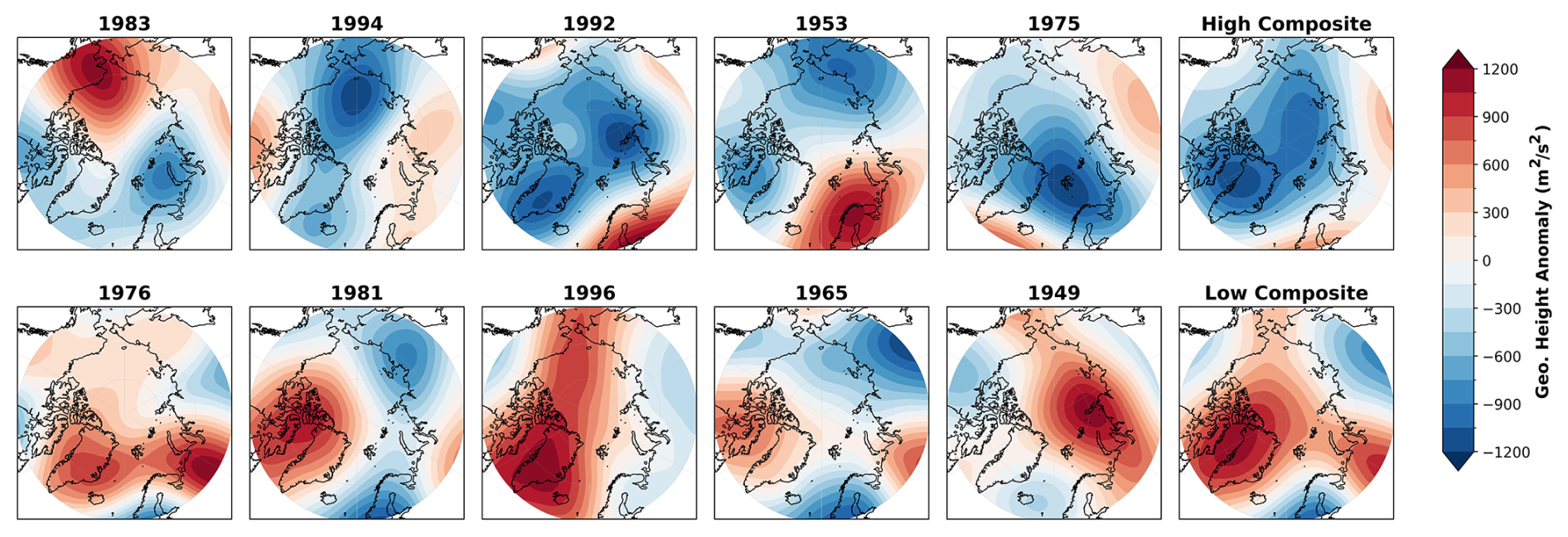
Figure A7 Geopotential height anomalies at 200 hPa in the Decembers preceding Januaries characterised by a high (upper row) and zero (lower row) number of stormy days in the UK Coast grid cell.

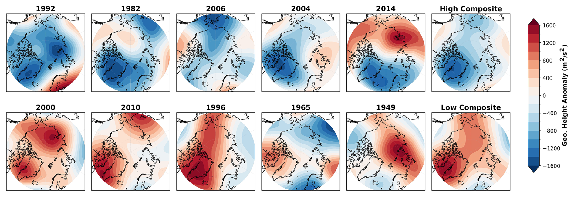
Figure A8 Geopotential height anomalies at 200 hPa in the Decembers preceding Januaries characterised by a high (upper row) and zero (lower row) number of stormy days in the German coast grid cell.

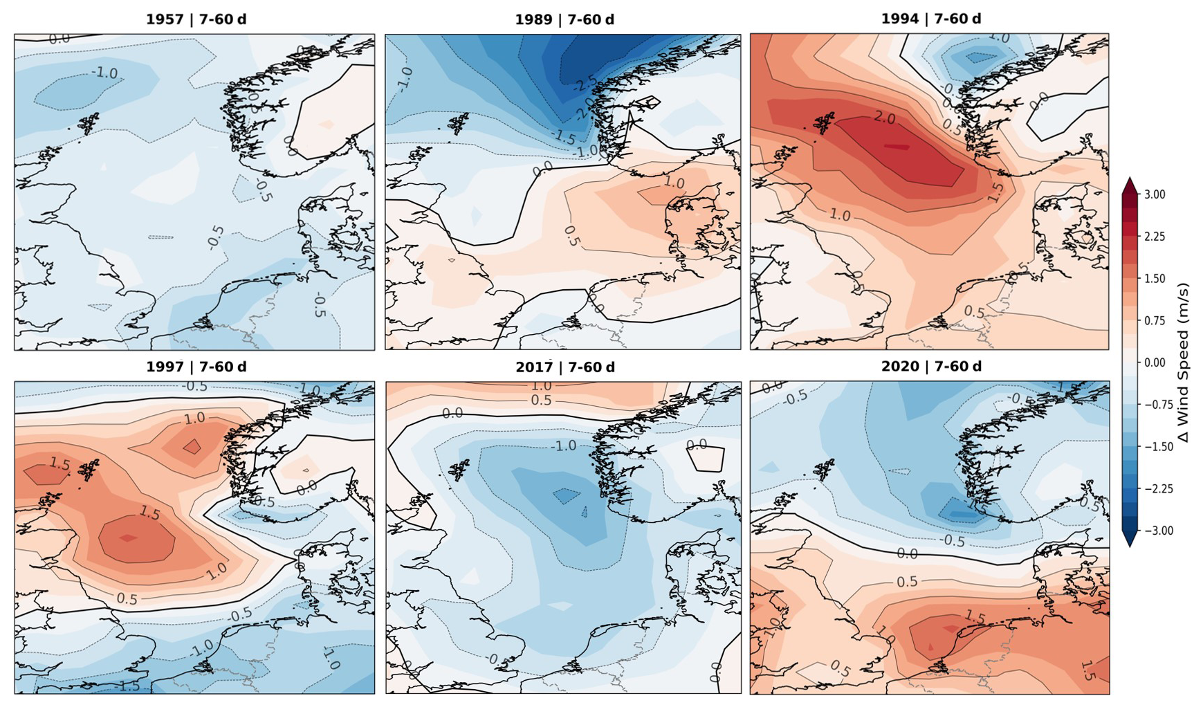
Figure A9 Temporal mean of 10 m wind speed response from ACE2 simulation (perturbed-controlled) for days 7–60 following initialisation. Shown are the difference fields for the cases of November 1957, 1989, 1994, 1997, 2017, and 2020. Warm colours indicate stronger near-surface winds in the perturbed run, while cool colours show reduced winds. For reference, the number of storms in the following Decembers was 2, 1, 2, 2, 2 and 2, respectively.