Multiscale assessment of Indian monsoon rainfall using ICON and CMIP6 model simulations

Indian Summer Monsoon (ISM) rainfall is organized across multiple timescales, from diurnal convection to synoptic disturbances, intraseasonal oscillations, and the seasonal mean. Climate models often show different levels of skill at each of these timescales, raising an important question: how do scale-dependent biases shape overall monsoon variability? Here, we assess a medium-resolution (40 km), non-hydrostatic global model (ICON) together with five hydrostatic CMIP6-class models (CNRM, MPI, GFDL, MIROC6, and IITM-ESM; 50–190 km resolution). All simulations are evaluated in AMIP configuration against high-resolution IMERG observations during 1998–2014, allowing isolation of atmospheric sources of rainfall bias. Rainfall errors are strongly scale-dependent and exhibit clear land–ocean contrasts. At the diurnal scale, ICON reproduces amplitudes over the continent with a relatively small bias (∼ 5 %–10 %), whereas MPI overestimates land diurnal amplitude by more than 150 % with premature triggering. The CNRM and GFDL show early daytime convection and weak nocturnal rainfall, while MIROC6 and IITM-ESM exhibit reduced diurnal amplitude linked to convective and resolution limitations. Over the Bay of Bengal, ICON overestimates diurnal amplitude (∼ 60 %) and variance (∼ 180 %), whereas CMIP6 models underestimate nocturnal oceanic variability (amplitude < 40 %, variance < 60 %). At synoptic timescales (2–7 d), models differ in their ability to sustain organized monsoon disturbances. ICON and GFDL maintain realistic spatial structure with moderate suppression, while MPI underestimates synoptic variance by up to ∼ 70 %–80 %. Other models either has weakened synoptic activity or redistribute variability toward intermediate (10–20 d) bands. Across the ensemble, the 20–100 d intraseasonal band is systematically underestimated (by ∼ 30 %–60 %) in the AMIP framework, suggesting that coupled ocean–atmosphere feedbacks, among other factors, contribute to maintaining monsoon intraseasonal oscillations. Seasonal rainfall patterns reflect the combined effect of these multiscale biases. Models that maintain a balanced variance distribution across diurnal, synoptic, and intraseasonal bands show improved seasonal structure, whereas distortions at intermediate frequencies contribute to amplitude and migration errors. These results indicate that credible monsoon simulation depends not only on seasonal-mean accuracy but also on physically consistent variability across timescales. A scale-aware diagnostic framework is therefore essential for improving convective triggering, mesoscale organization, boundary-layer processes, and air–sea coupling in climate models.

1 Introduction

Accurate forecasting of precipitation over the Indian subcontinent has long remained an enduring scientific challenge, with growing demand for skillful predictions not only at all-India level but scaling down till sub-district level. Achieving such high spatial fidelity in rainfall prediction requires forecast models to faithfully reproduce all the fundamental scales of variability of the Indian summer monsoon, ranging from the diurnal convective cycle to synoptic disturbances, intraseasonal oscillations (ISOs), and the seasonal mean rainfall. These interacting scales form the backbone of monsoon dynamics, collectively governing how convection initiates, organizes, and propagates across the subcontinent (Webster et al., 1998; Goswami, 2005). Their interplay determines not only the timing and intensity of rainfall, but also the limits of its predictability on different timescales (e.g. Turner and Annamalai, 2012). Yet, despite remarkable progress in model physics, resolution, and data assimilation over the past decades, systematic errors in simulating precipitation remain pervasive across generations of global climate models (Sperber et al., 2013), particularly in regions such as Central India (CI) and Bay of Bengal (BoB) where multiscale convective coupling and ocean–land–atmosphere interactions dominate.

Rainfall variability during the Indian summer monsoon arises from a hierarchy of interacting physical modes. At the shortest timescale, the diurnal cycle represents one of the most fundamental features of tropical convection, exerting strong control on the timing and organization of rainfall over both land and ocean (Johnson, 2011). Over India, the diurnal cycle is strongly modulated by orography, land–sea thermal contrasts, and large-scale circulation, leading to pronounced regional heterogeneity that has recently been observed to experience significant spatial and temporal phase shifts (e.g. Basu, 2007; Sen Roy and Balling, 2007; Sahany et al., 2010; Chutia et al., 2025, etc.). The next tier of variability, the synoptic disturbances on 2–7 d timescales, comprises monsoon low-pressure systems (LPS) that form primarily over the BoB and propagate north-westward, delivering substantial rainfall to CI (Godbole, 1977; Sikka, 1977; Patwardhan et al., 2020; Hunt and Turner, 2022). These systems are dynamically linked to instabilities within the monsoon trough, including moist baroclinic processes as well as barotropic growth associated with horizontal wind shear, with surface heat fluxes providing additional energetic support in some regimes (Shukla, 1987; Goswami et al., 1980; Mak, 1987; Diaz and Boos, 2021). At longer timescales, the ISOs emerge as dominant modes of low-frequency variability, characterized by quasi-periodic fluctuations in convection and rainfall on 10–20 and 30–60 d bands (Krishnamurti and Bhalme, 1976; Yasunari, 1979; Sikka and Gadgil, 1980). Together, these two modes account for nearly 90 % of the total intraseasonal variability in monsoon rainfall (Annamalai and Slingo, 2001). The 30–60 d mode, typically originates over the equatorial Indian Ocean and propagates northward, while the 10–20 d mode often initiates over the South China Sea and propagates north-westward (Webster et al., 1998; Wang, 2006). Collectively, these diurnal, synoptic, and intraseasonal modes form an interconnected cascade that shapes the structure, evolution, and predictability of the Indian summer monsoon (Krishnamurti and Subrahmanyam, 1982).

Among these multiscale physical modes, the diurnal cycle of precipitation serves as a fundamental testbed for assessing a model's ability to reproduce key convective and radiative processes (Lin et al., 2000; Trenberth et al., 2003; Dai and Trenberth, 2004). Despite major progress across generations of the Coupled Model Intercomparison Project (CMIP), models continue to exhibit persistent biases in simulating tropical diurnal rainfall. Evaluations of CMIP6 models have revealed that the timing of peak rainfall is typically 3–5 h too early over land and 1–2 h too early over oceans compared with high-quality satellite and gauge observations (Tang et al., 2021, 2022; Christopoulos and Schneider, 2021). Over land, many models exhibit premature initiation of convection, producing rainfall peaks several hours earlier than observed and leading to overly frequent but weak precipitation, the so-called “drizzling bias” (Chen et al., 2021). This behaviour arises from the inability of conventional cumulus parameterization schemes to realistically simulate the morning growth of the non-precipitating convective boundary layer (Betts and Jakob, 2002; Bechtold et al., 2004) and the associated buildup of convective available potential energy (CAPE; Folkins et al., 2014; Rio et al., 2009; Tawfik et al., 2017). Over oceans, the diurnal amplitude is often underestimated due to the absence of subdaily air–sea coupling and diurnal sea surface temperature (SST) variability over the Indian subcontinent (Baranowski et al., 2019; Peng and Chen, 2024), these problems are amplified by strong land–sea thermal contrasts and orographic influences, where models often fail to reproduce the observed afternoon peaks and propagating MCSs over the BoB (Kilpatrick et al., 2017; Seo et al., 2014). Importantly, these deficiencies extend beyond the diurnal scale. CMIP6 models continue to underrepresent the intensity and organization of monsoon LPSs and ISOs (Sperber et al., 2013; Konda and Vissa, 2022; Jiang et al., 2020). Many models struggle to simulate the amplitude, northward propagation, and phase coherence of the 10–20 and 30–60 d ISOs, indicating systematic errors in convective–dynamical coupling across scales (Rajendran et al., 2022). These results suggest that precipitation biases are not isolated at individual time scales but may reflect misrepresentation of scale interactions and convective organization. A systematic multiscale evaluation is therefore essential to determine whether model errors arise independently at each temporal mode or cascade across interacting scales.

Accurate simulation of monsoon rainfall fundamentally depends on the representation of vertical motion and its coupling with moist convection. In the tropics, vertical velocity governs moisture convergence, buoyancy generation, and latent heat release, thereby controlling the initiation, intensity, and organization of deep convection (Emanuel, 1994; Houze, 2004). The vertical momentum equation may be expressed as

$$\begin{array}{}\text{(1)}& {\displaystyle \frac{\mathrm{D}w}{\mathrm{D}t}}=-{\displaystyle \frac{\mathrm{1}}{\mathit{\rho }}}{\displaystyle \frac{\partial p^{\prime }}{\partial z}}+B+F,\end{array}$$

where $\mathrm{D}w/\mathrm{D}t$ denotes the vertical acceleration, ρ is the air density, p^′ represents the perturbation pressure, B denotes buoyancy, and F represents subgrid-scale forcing terms. This formulation highlights the central role of vertical acceleration in convective dynamics. In hydrostatic general circulation models (GCMs), vertical motion is diagnostically constrained under the hydrostatic approximation, which filters vertical acceleration and may limit the representation of mesoscale convective circulations and gravity-wave–convection interactions. In contrast, non-hydrostatic dynamical cores explicitly solve the vertical momentum equation, allowing a more dynamically consistent treatment of vertical accelerations associated with organized convection and mesoscale systems (Satoh et al., 2008; Stevens et al., 2019). Given that monsoon precipitation variability across diurnal to intraseasonal time scales is tightly linked to convective organization, the fidelity of vertical motion representation may substantially influence simulated multiscale rainfall characteristics however, improvements in physical parameterizations and model coupling are equally important.

Recent advances in atmospheric modelling include the development of the ICOsahedral Nonhydrostatic (ICON) model (Zängl et al., 2015; Dipankar et al., 2026), which employs a non-hydrostatic dynamical framework. While convection remains parameterized at typical climate-model resolutions, the explicit treatment of vertical acceleration and improved dynamical consistency may influence the simulation of tropical precipitation variability. A concise assessment of whether such dynamical formulation translates into improved multiscale precipitation representation over the Indian monsoon region remains lacking. Therefore, we employ the ∼ 40 km global configuration of ICON model as a practical test case to evaluate the added value of non-hydrostatic dynamics for simulating Indian summer monsoon variability. At ∼ 40 km resolution, ICON provides a computationally feasible intermediate configuration between conventional hydrostatic climate models and emerging kilometre-scale global simulations. This enables a comparative assessment of multiscale monsoon rainfall biases across model configurations, rather than a controlled isolation of dynamical-core or resolution effects.

In this study, we evaluate precipitation characteristics across diurnal, synoptic, intraseasonal, and seasonal scales using simulations from ICON and selected CMIP6 atmospheric models, including CNRM-CM6-1-HR, MPI-ESM1.2-HR, GFDL-CM4, MIROC6, and the IITM Earth System Model (IITM-ESM). All simulations are analysed in their Atmospheric Model Intercomparison Project (AMIP) configuration to compare monsoon convection under prescribed sea surface temperature boundary conditions. The novelty of this work lies in providing a unified, scale-aware assessment of how a medium-resolution non-hydrostatic global model performs relative to state-of-the-art hydrostatic CMIP6 models in simulating the full spectrum of Indian monsoon rainfall variability, with particular emphasis on identifying scale-dependent strengths, deficiencies, and the consistency of model errors across the temporal hierarchy across key monsoon subregions. The paper is organized as follows. Section 2 describes the datasets, models, and experimental design. Section 3.1 evaluates the diurnal characteristics of monsoon rainfall, while Sect. 3.2 examines synoptic and intraseasonal variability using variance and spectral diagnostics. Section 3.3 shows the error in the seasonal scale and also assess scale-wise error characteristics across models. Finally, Sect. 4 summarizes the main findings and discusses their implications for future non-hydrostatic global modelling of the Indian monsoon.

2 Data and Methodology

2.1 Observation

IMERG

Precipitation observations are obtained from the Integrated Multi-satellite Retrievals for the Global Precipitation Measurement (IMERG) Version 07 Final Run product (Huffman et al., 2023), spanning 1998–2023. IMERG is developed under the Global Precipitation Measurement (GPM) mission and provides globally consistent, gauge-adjusted precipitation estimates by merging passive microwave observations from a constellation of ten satellites including dual-frequency precipitation radar, as well as a multi-channel GPM Microwave Imager. The Final Run product incorporates monthly gauge corrections and retrospective calibration, making it suitable for climate-scale analysis. Previous evaluations over the Indian region suggest that IMERG reasonably captures large-scale monsoon rainfall characteristics as well as sub-daily variability, supporting its application in studies of monsoon dynamics across multiple temporal scales (Murali Krishna et al., 2017; Ponukumati et al., 2023). However, some systematic biases in rainfall intensity and reduced accuracy during short-duration extreme events have been reported, particularly over complex terrain and at finer temporal scales. IMERG provides near-global coverage (90° S to 90° N) at high spatial resolution (0.1° × 0.1°) and a temporal resolution of 30 min, enabling robust assessment of precipitation variability from diurnal to seasonal time scales, which is particularly relevant for investigating multi-scale variability of the Indian summer monsoon.

2.2 Models

2.2.1 ICON

ICON model was developed through a joint initiative of the German Weather Service (DWD) and the Max Planck Institute for Meteorology (MPI-M) to provide a unified framework for numerical weather prediction and climate modelling (Zängl et al., 2015). ICON was explicitly designed to transition toward a fully non-hydrostatic dynamical core capable of resolving cloud-scale processes (Zängl et al., 2015; Wan et al., 2013). This non-hydrostatic core employs prognostic density and virtual potential temperature to ensure local mass conservation and uses a stable two-time-level predictor-corrector scheme that performs robustly over steep orography, an essential requirement for monsoon regions characterized by strong terrain–convection interactions. Very recently, ICON has also been adapted for exascale computing through GPU acceleration and domain-specific languages such as GT4Py, enabling multi-year global simulations at kilometer-scale resolution in experimental configurations (Lapillonne et al., 2026; Prein et al., 2026). The present set up uses ICON EXCLAIM version with a GT4Py dycore to run the experiments (Dipankar et al., 2026).

Model Configuration

The simulation was performed on the ALPS high-performance computing (HPC) infrastructure of the Swiss National Computing Center using 22 GPU nodes (NVIDIA GH200) for model integration and two dedicated nodes for input/output operations. A horizontal grid spacing of 40 km was used with 120 terrain-following vertical levels based on the smooth level vertical (SLEVE) coordinate (Leuenberger et al., 2010). The numerical time step for dynamics was 180s. Physical parameterizations were called at varying frequencies: convection, cloud cover, subgrid-scale orography, and non-orographic gravity wave drag schemes every 12 min, and radiation every 30 min.

Initial and Boundary Conditions

The simulation was initialized from European Center for Medium-Range Weather Forecasts (ECMWF) operational analysis on 1 January 1979 at 00:00 UTC, and run continuously until 1 January 2022 at 00:00 UTC. Sea surface temperature and sea ice cover were prescribed from the PCMDI AMIP II dataset (Taylor et al., 2000), updated monthly. The global aerosol climatology was provided by the Max-Planck-Institute Aerosol Climatology version 2 (MAC-v2) at 1° resolution (Kinne, 2019). Static surface fields (topography, land cover, vegetation, and soil properties) were prepared using the External Parameters for Numerical Weather Prediction and Climate Applications software (Asensio et al., 2020).

Physics Parameterizations

Deep and shallow convection were parameterized using the Tiedtke-Bechtold bulk mass flux scheme (Bechtold et al., 2001). Cloud microphysics followed a single-moment scheme for cloud water, cloud ice, snow, and rain (Hong and Lim, 2006). Land surface processes were simulated with the TERRA soil–vegetation–atmosphere transfer model (Schulz and Vogel, 2020) using eight soil levels. Turbulent transport in the boundary layer and surface exchange was represented using a turbulent kinetic energy-based scheme with a second-order closure (Raschendorfer et al., 2003).

2.2.2 CMIP6-AMIP

To provide a comprehensive intercomparison framework, we analyze atmospheric simulations from five CMIP6 models: CNRM-CM6-1-HR, MPI-ESM1.2-HR, GFDL-CM4, MIROC6, and the IITM-ESM. For brevity, these models are hereafter referred to as CNRM, MPI, GFDL, and MIROC, respectively, while IITM-ESM is retained as IITM-ESM. These models are selected primarily based on the availability of 3-hourly temporal resolution precipitation output, which is required to resolve the diurnal cycle and to apply a consistent multiscale rainfall analysis. All models are evaluated in their AMIP configuration, which prescribes observed sea surface temperatures and sea ice concentrations. The selected models span a range of horizontal resolutions (∼ 50–190 km), dynamical cores (hydrostatic spectral, finite-volume, and semi-Lagrangian formulations), and convection parameterization schemes (details provided in Table 1). For better understanding models having horizontal resolution less (more) than 100 km is considered as higher (coarser) resolution models. Therefore, the selected CMIP6 models are used as a structurally diverse set of available AMIP simulations for comparative evaluation, rather than as an exhaustive CMIP6 ensemble.

All model–observation bias and skill diagnostics are computed for the common IMERG–model overlap period of 1998–2014 to ensure temporal consistency across datasets. Climatological diagnostics used to illustrate the broad spatial structure of rainfall variability are computed using the full available period of each dataset, with the analysis period stated explicitly in the corresponding figure captions.

Müller et al. (2025)Dipankar et al. (2026)(Seifert, 2008)Tiedtke, 1989Bechtold et al., 2008Voldoire (2019)Voldoire et al. (2019)Bretherton et al. (2004)Piriou et al., 2007Guérémy, 2011Lopez (2002)Jungclaus et al. (2019)Müller et al. (2018)Guo et al. (2018)Held et al. (2019)Chikira and Sugiyama (2010)Hajima et al. (2020)Tatebe et al. (2019)Park and Bretherton (2009)Narayanasetti et al. (2020)(Zhao and Carr, 1997)Krishnan et al. (2019)(Han and Pan, 2011)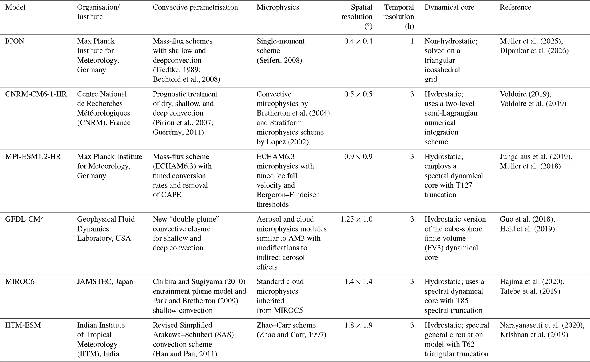

Table 1 Description of models used in this study.

2.3 Methodology

2.3.1 Harmonic Analysis

Harmonic analysis provides a compact framework to quantify the amplitude and timing of phase-locked diurnal and semi-diurnal rainfall variability. It has been applied in atmospheric precipitation studies to diagnose land–ocean phase contrasts, orographic effects, propagation features, and model timing biases, including over North America (Wallace, 1975; Dai et al., 1999), the Indian monsoon region (Sahany et al., 2010; Johnson, 2011), and in recent diurnal-cycle evaluations of CMIP6 models (Tang et al., 2021, 2022).

The fundamental form of the harmonic equation used in this analysis is expressed in the combined sine–cosine form:

$$\begin{array}{}\text{(2)}& P=\stackrel{\mathrm{‾}}{P}+\sum _{i=\mathrm{1}}^{n/\mathrm{2}}\left[a_i\cos \left({\displaystyle \frac{\mathrm{2}\mathit{\pi }it}{T}}\right)+b_i\sin \left({\displaystyle \frac{\mathrm{2}\mathit{\pi }it}{T}}\right)\right]\end{array}$$

where P represents the precipitation data (ICON, CNRM, MPI, GFDL, MIROC, IITM-ESM and IMERG), and $\stackrel{\mathrm{‾}}{P}$ denotes the mean value of n observations. The subscript i indicates the harmonic number, corresponding to the first, second, up to the nth harmonics of the period T (for diurnal analysis, T = 24 h). The variable t represents time in hours (for IMERG data: 00:00, 00:30, 01:00, …, 23:00, 23:30).

The maximum number of harmonics that can represent the full series is $n/\mathrm{2}$. For example, half-hourly GPM-IMERG data, consisting of 48 observations within one period T, can be represented by 24 harmonics. Similarly, ICON datasets with 1-hourly time steps (24 observations) can be represented by 12 harmonics, while other models with 3-hourly time steps (8 observations) can be represented by 4 harmonics.

The first (i = 1) and second (i = 2) harmonics represent the diurnal (24 h) and semi-diurnal (12 h) variability, respectively. The coefficients a_i and b_i correspond to the coefficients of the cosine and sine components of each harmonic, respectively. The amplitude (A_i) and phase (Φ_i) are defined as:

$$\begin{array}{}\text{(3)}& {\displaystyle }{A}_i=\sqrt{a_i^{\mathrm{2}}+b_i^{\mathrm{2}}}\text{(4)}& {\displaystyle }{\mathrm{\Phi }}_i={\tan }^{-\mathrm{1}}\left({\displaystyle \frac{b_i}{a_i}}\right)\end{array}$$

Here, A_i represents the diurnal amplitude (the magnitude of maximum rainfall variation), and Φ_i denotes the phase (the timing of the maximum rainfall) for the ith harmonic.

For a sinusoidal harmonic component, the variance explained by the ith harmonic is related to its amplitude as

$$\begin{array}{}\text{(5)}& {\mathit{\sigma }}_i^{\mathrm{2}}={\displaystyle \frac{a_i^{\mathrm{2}}+b_i^{\mathrm{2}}}{\mathrm{2}}}={\displaystyle \frac{A_i^{\mathrm{2}}}{\mathrm{2}}}\end{array}$$

Thus, variance scales quadratically with amplitude, so a moderate amplitude bias can produce a larger variance bias. Here, amplitude diagnostics describe the strength of phase-locked components, while variance diagnostics quantify the distribution of rainfall variability across temporal bands.

2.3.2 Empirical orthogonal function analysis

To examine the dominant spatial structures of diurnal rainfall variability, Empirical Orthogonal Function (EOF) analysis (Lorenz, 1956) is applied to rainfall anomalies obtained by removing the daily mean at each grid point. The analysis is performed over the domain shown in Fig. 2. The leading EOF modes represent coherent patterns of the diurnal cycle, including stationary responses over land and propagating signals associated with coastal and orographic convection. Model fidelity is evaluated by comparing the spatial structure and explained variance of these modes with IMERG observations.

In EOF analysis, the spatial eigenvectors represent the dominant spatial patterns of variability, while the associated principal components (PCs) describe their temporal evolution. Such a decomposition allows the separation of spatial structures and temporal variability of rainfall, facilitating the identification of distinct diurnal regimes. Model performance can further be assessed by comparing the temporal correlation of PCs and the spatial errors of EOF patterns between observations and simulations (Huang and Wang, 2017).

3 Results and Discussion

3.1 Assessment of diurnal scale variability in models with observation

The diurnal cycle of precipitation provides a stringent benchmark for evaluating model fidelity, as it reflects the coupled evolution of boundary-layer thermodynamics, convective triggering, cloud–radiative feedback, and mesoscale organization (Johnson, 2011). Over the Indian monsoon region, the diurnal signal is strongly modulated by orography, land–sea thermal contrasts, and the background monsoon circulation (Sahany et al., 2010). Accurate simulation of both the amplitude and phase of the diurnal harmonic is therefore essential to check how models simulate convective processes across heterogeneous terrain and adjacent oceanic regions.

3.1.1 Diurnal Amplitude and Phase

The climatological mean diurnal amplitude of rainfall during the Indian summer monsoon for June, July, August, September (JJAS) period for 1979–2014 from ICON and five CMIP6 models (CNRM, MPI, GFDL, MIROC, and IITM-ESM) is evaluated against IMERG (Fig. 1). ICON captures the large-scale spatial distribution of the observed diurnal amplitude over the Indian landmass and adjoining oceans (Fig. 1a, g), but with systematic overestimation along the Himalayan foothills, the Arakan Yoma range, and the Western Ghats. Over the eastern equatorial Indian Ocean, particularly within the Oceanic Tropical Convergence Zone (OTCZ), ICON simulates nearly double the observed diurnal amplitude, indicating enhanced diurnal modulation of oceanic convection.

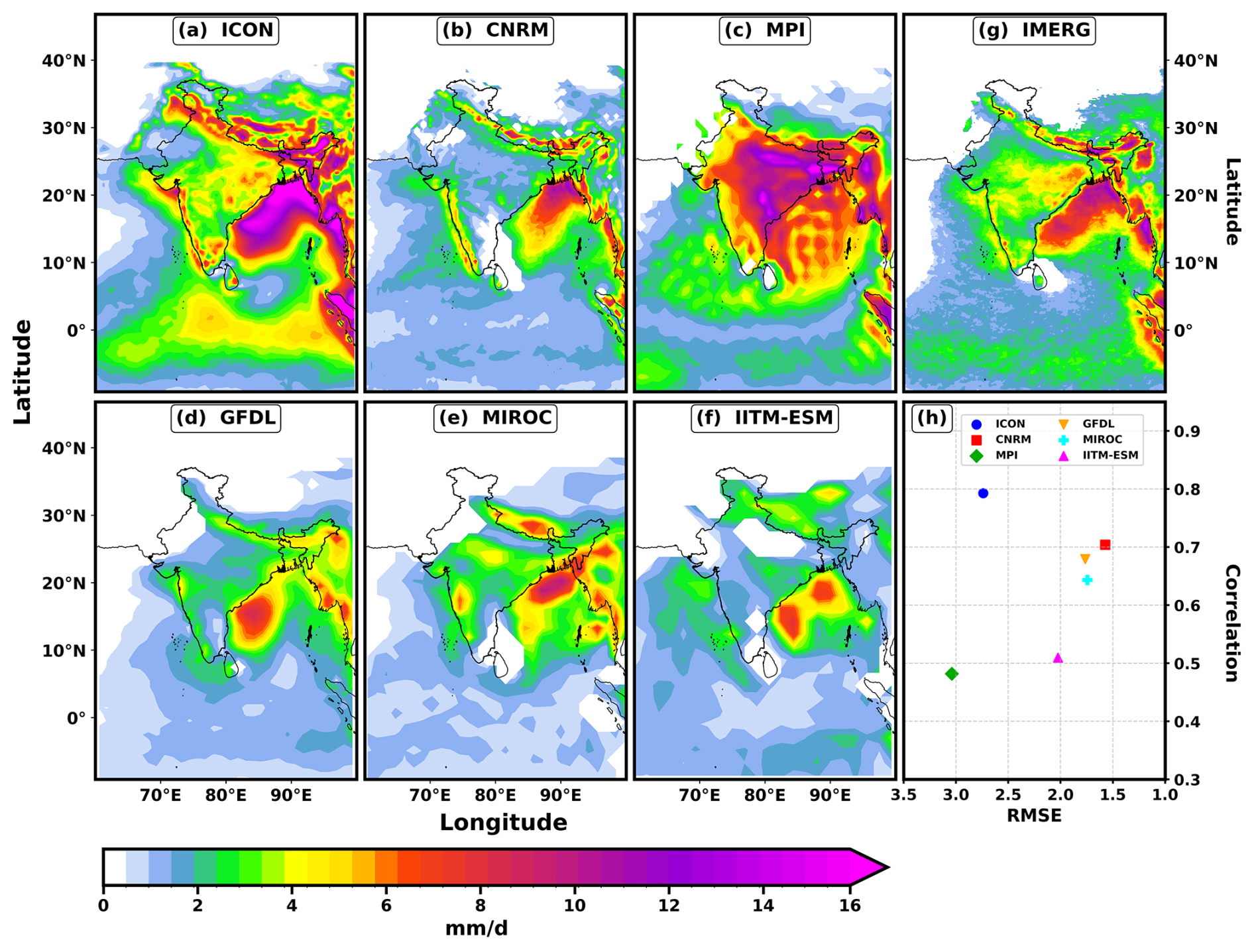
Figure 1 Climatological mean diurnal amplitude of precipitation (mm d⁻¹) during the Indian summer monsoon season (JJAS) from (a–f) ICON, CNRM, MPI, GFDL, MIROC, and IITM-ESM model simulations, with (g) IMERG as the observational reference. Panel (h) shows the relationship between model performance metrics, with a scatterplot of pattern correlation versus root-mean-square error (RMSE) for all models relative to IMERG.

Among CMIP6 high-resolution models, CNRM reasonably reproduces the spatial pattern of diurnal amplitude but underestimates its magnitude, especially over CI and the equatorial Indian Ocean (Fig. 1b). MPI shows pervasive overestimation across the entire domain (Fig. 1c), characterized by unrealistic wave-like artifacts. Coarser-resolution models such as GFDL (Fig. 1d), MIROC (Fig. 1e), and IITM-ESM (Fig. 1f) fail to adequately resolve the smaller topographic features resulting in diurnal maxima along the Western and Eastern Ghats, appear fragmented rather than forming continuous bands as seen in IMERG. Such fragmentation and reduced intensity over complex terrain are consistent with earlier findings that coarse horizontal resolution and parameterized convection can smooth sharp precipitation gradients and weaken orographic rainfall contrasts (e.g. Basu, 2007; Krishnamurti et al., 2007). Despite their coarser resolution, GFDL and MIROC capture the broad spatial pattern of diurnal amplitude. GFDL displays a southwestward shift of the BoB maximum, whereas the characteristic diurnal maximum over the northern Gangetic plains is largely absent in IITM-ESM.

The RMSE, pattern correlation (PCC) summary (Fig. 1h), computed over the study domain shown in the Fig. 1a–g, highlights a trade-off between spatial fidelity and magnitude bias. ICON shows the highest PCC (∼ 0.8) but relatively larger RMSE (∼ 2.7 mm d⁻¹), reflecting amplitude overestimation. CNRM, GFDL, and MIROC exhibit moderate correlation (∼ 0.6–0.7) with lower RMSE (1.5–1.8 mm d⁻¹), while MPI and IITM-ESM show weaker correlation (∼ 0.5). IITM-ESM, despite its coarser resolution, maintains lower RMSE (∼ 2.0 mm d⁻¹) than ICON due to systematic amplitude underestimation. These results indicate that improved spatial agreement does not necessarily correspond to reduced mean error, and that amplitude bias exerts a dominant influence on RMSE across models.

The spatial pattern of diurnal rainfall bias highlights regionally organized systematic errors and provides additional context to the diurnal amplitude structure. ICON exhibits relatively modest bias over most continental regions but shows pronounced positive bias over oceanic convective zones and along the Himalayan foothills (Fig. 2a). Notably, these regions are characterized by late-night to early-morning diurnal maxima in observations. The systematic overestimation in these areas suggests difficulties in representing convection that peaks during nocturnal or early-morning hours, when boundary-layer thermodynamics and large-scale dynamical forcing differ substantially from daytime conditions. Further, in ICON simulations the positive bias over the northern BoB is amplified. This region is known for strong diurnal propagation and organized mesoscale convection (e.g. Johnson, 2011; Fujinami et al., 2005) and misrepresentation of these physical processes likely contributes to the enhanced amplitude bias in ICON. Among the CMIP6 models, MPI exhibits the most pronounced overestimation of diurnal amplitude across nearly the entire domain, with only localized underestimation over parts of the northern and western BoB (Fig. 2c). In contrast, CNRM, GFDL, MIROC, and IITM-ESM predominantly underestimate diurnal amplitude over both land and ocean, indicating a systematic negative bias across much of the monsoon region.

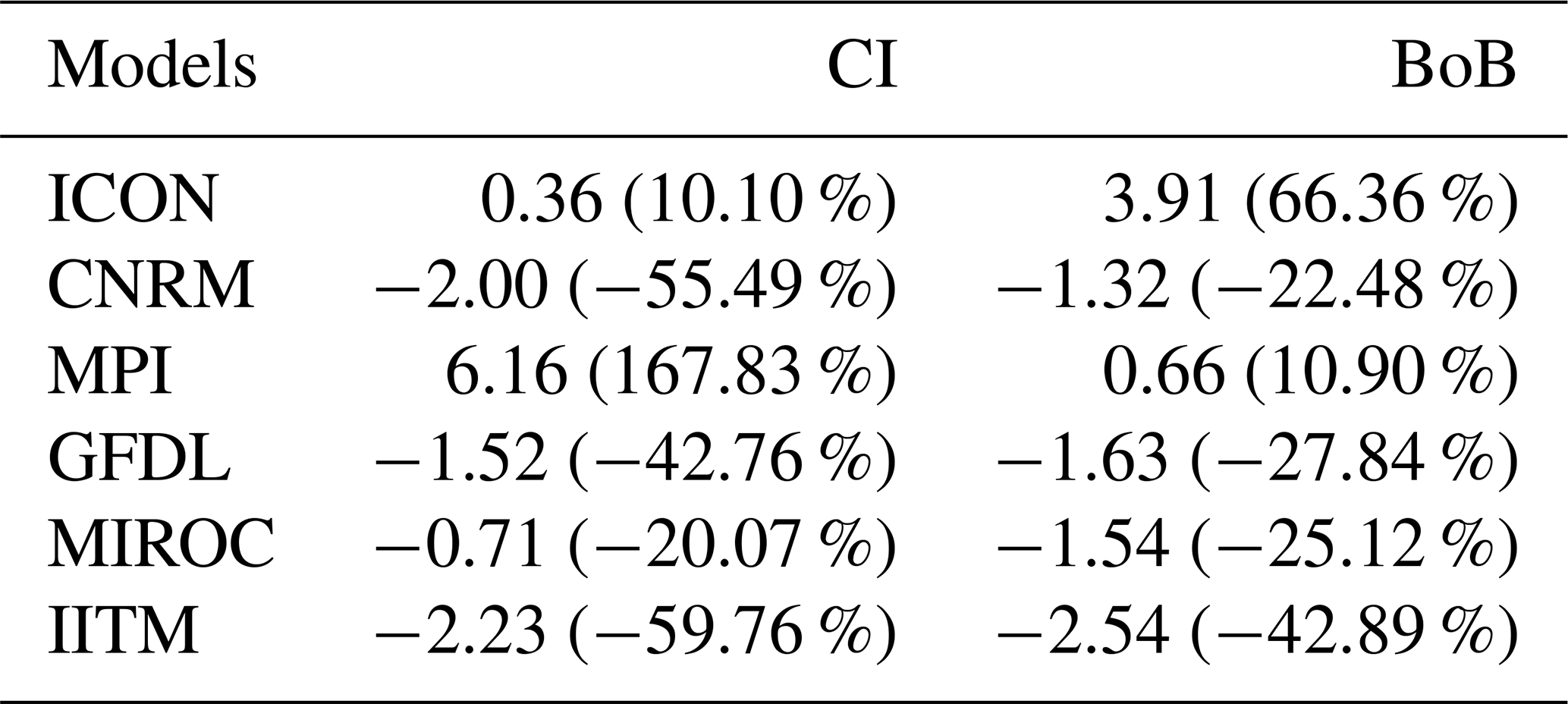
Regional means are calculated over the CI land region (16.5–26.5° N, 74.5–86.5° E; Goswami et al., 2006) and the BoB ocean region (12–22.5° N, 80–99° E; Pokhrel et al., 2018b), as shown in Fig. 2f, and are summarized in Table 2 using both absolute and percentage biases relative to IMERG. ICON shows the smallest positive bias over CI (+0.36 mm d⁻¹; 10.10 %), whereas MPI exhibits the largest positive bias over land (+6.16 mm d⁻¹; 167.83 %). In contrast, over the BoB, ICON shows the largest positive bias (+3.91 mm d⁻¹; 66.36 %), while CNRM, GFDL, MIROC, and IITM-ESM show negative biases ranging from −22.48 % to −42.89 %. Thus, the percentage-bias estimates reinforce the land–ocean contrast: ICON performs well over CI in relative terms, but its diurnal amplitude is substantially overestimated over the BoB. These regional biases show that ICON’s improved spatial organization and phase representation do not translate into uniformly smaller amplitude errors. In particular, its large positive bias over the BoB indicates a substantial overestimation of oceanic diurnal rainfall amplitude, whereas several CMIP6 models show smaller absolute biases over this region.

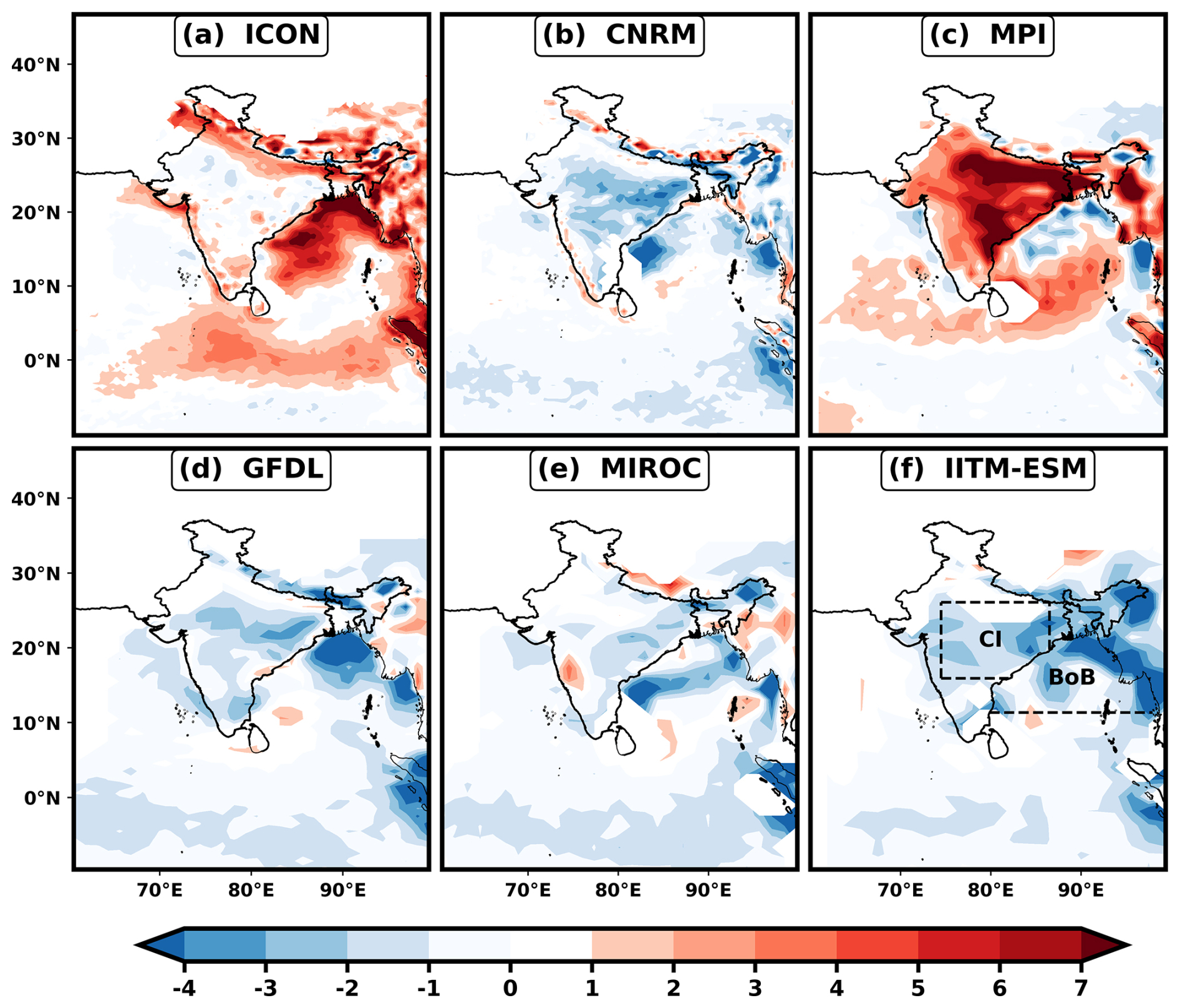
Figure 2 Spatial distribution of JJAS climatological mean diurnal precipitation amplitude bias (mm d⁻¹) relative to IMERG for (a–f) ICON, CNRM, MPI, GFDL, MIROC and IITM-ESM. The two representative regions Central India (CI), and the Bay of Bengal (BoB) used for regional bias analysis (Table 2) are indicated in panel (f). The boxes are bounded by land boundaries and dashed outlines such that CI excludes oceanic grid points and BoB excludes land grid points.

Table 2 Mean diurnal rainfall bias (mm d⁻¹) averaged over the Central India (CI) and Bay of Bengal (BoB) boxes, as defined in Fig. 2f.

The normalized evening (12:00–23:00 LT) minus morning (00:00–11:00 LT) rainfall is used here as a climatological diagnostic to highlight the canonical land–ocean phase contrast of the monsoon region (Fig. 3). In IMERG (Fig. 3g), most of the Indian landmass exhibits a dominant afternoon–evening maximum, whereas adjacent oceanic regions show prevailing morning rainfall, consistent with earlier satellite analyses (Johnson, 2011). Two notable exceptions emerge: (i) the Himalayan foothills, where rainfall peaks during late night to early morning due to nocturnal low-level convergence and orographic effects (Barros and Lang, 2003; Fujinami et al., 2005; Chen, 2020), and (ii) the central BoB, where an afternoon maximum replaces the typical oceanic morning peak, associated with westward-propagating mesoscale convective systems (MCSs) and gravity-wave modulation (Johnson, 2011).

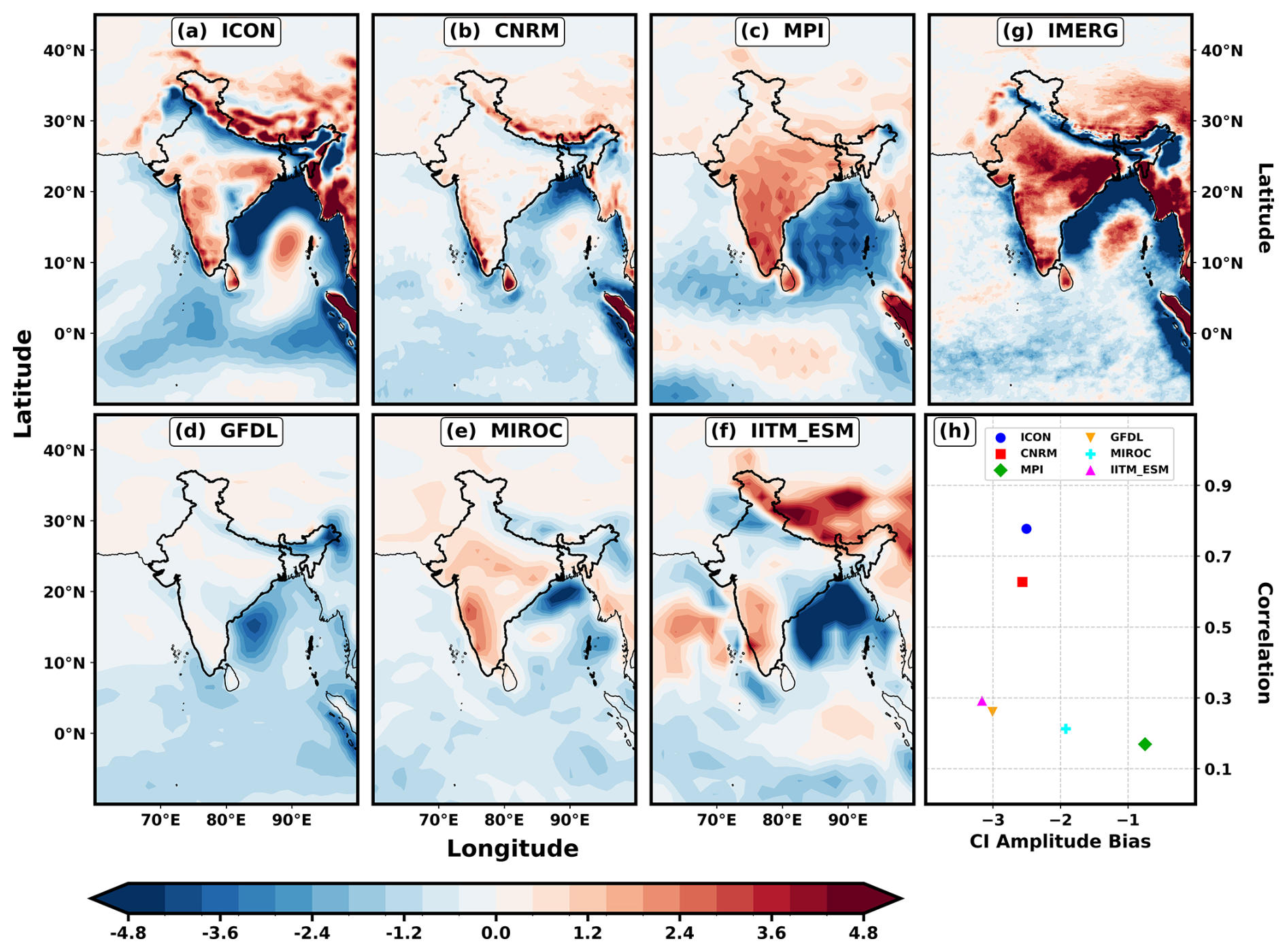
Figure 3 Climatological mean JJAS evening (12:00–23:30 LT) minus morning (00:00–11:30 LT) precipitation, normalized by the JJAS mean rainfall, from (a–f) ICON, CNRM, MPI, GFDL, MIROC, and IITM-ESM model simulations and (g) IMERG observations. The models are shown for 1979–2014, while IMERG is shown for its available observational period used in this analysis. Panel (h) shows the pattern correlation of each model with IMERG and the Central India (CI) mean climatological difference between models and IMERG. Precipitation is expressed in mm d⁻¹.

ICON reproduces the large-scale land–ocean contrast and the key exception regions with relatively high spatial agreement (PCC = 0.79; Fig. 3a). However, the Himalayan morning maximum is displaced southward and an additional morning signal emerges along the eastern Indian coast, leading to a substantial CI phase-related amplitude bias (−2.5 mm d⁻¹). This trade-off between spatial correlation and regional bias is evident in the CI bias–PCC scatter plot (Fig. 3h). Among the CMIP6 models, CNRM shows a comparable magnitude of CI bias despite lower pattern correlation (0.6). In contrast, MPI despite deficiencies in representing regional phase reversals as indicated by the lowest PCC (0.2), it exhibits a smaller CI bias (−0.8 mm d⁻¹), followed by MIROC (−0.2 mm d⁻¹), indicating that reduced structural fidelity does not necessarily imply larger regional amplitude error. Among the remaining models, GFDL and IITM-ESM show very weak diurnal contrast, with limited skill in reproducing the continental timing, as indicated by lower PCC and higher CI bias. IITM-ESM additionally exhibits a southward shift of the BoB signal and an unrealistic evening dominance over parts of the Arabian Sea. MIROC performs comparatively better among the coarser models, capturing the primary contrast and regional phase behaviour, though with reduced intensity. Overall, inter-model differences primarily reflect their ability to capture regional phase reversals and the sharp land–ocean transition, which are critical characteristics of the monsoon diurnal cycle. The subsequent discussion on the spatial phase biases will make it more clear.

To complement the spatial diagnostics, the composite diurnal cycle over CI and the BoB is examined (Fig. S1 in the Supplement). ICON reproduces the observed diurnal cycle over CI with realistic amplitude and minimal phase error, whereas most CMIP6 models exhibit reduced amplitudes and earlier peaks, with MPI showing a pronounced overestimation of amplitude and an unrealistic early peak. Over the BoB, ICON overestimates the diurnal amplitude but captures the phase more accurately than other models, which generally display weaker amplitudes and delayed peaks. The amplitude–phase error characteristics further confirm that ICON performs comparatively better in phase representation across both regions, despite residual amplitude biases, particularly over the ocean. These regional characteristics are further reflected in the spatial distribution of phase biases discussed below.

The diurnal phase of precipitation over the Indian subcontinent remains a significant challenge for state-of-the-art climate models, with both ICON and CMIP6 models exhibiting pervasive systematic biases in rainfall timing (Fig. 4a–f). Over most of the Indian landmass, models tend to produce rainfall prematurely, with an early bias up to 9 h. ICON (Fig. 4a) shows the smallest early bias, whereas MPI (Fig. 4c) exhibits the largest. Along the Himalayan foothills, ICON displays a delayed phase, particularly over the western Gangetaic basin, a feature absent in other models. The relatively reduced early bias in ICON and CNRM suggests some sensitivity to horizontal resolution, while coarser models such as GFDL and MIROC display widespread premature initiation. IITM-ESM, despite its coarse resolution, shows comparatively weaker early bias over parts of CI. Premature convection over land has been widely attributed to deficiencies in convective parameterization schemes, which trigger rainfall near local noon rather than the observed late-afternoon peak (Jha et al., 2022; Sahany, 2009). This early triggering limits the buildup of CAPE, leading to weakened and temporally displaced rainfall maxima (Hunt et al., 2022; Krishnamurti et al., 2007; Krishna et al., 2021). Over the surrounding oceans, models generally exhibit a late phase bias of up to 12 h, consistent with excessive persistence of stratiform precipitation (Pokhrel and Sikka, 2013). The BoB differs from this general oceanic behaviour, with most models producing rainfall too early. ICON shows an average 3 h early bias over the BoB, increasing to 6 h in MPI and GFDL, while MIROC and IITM-ESM display smaller, spatially confined early biases.

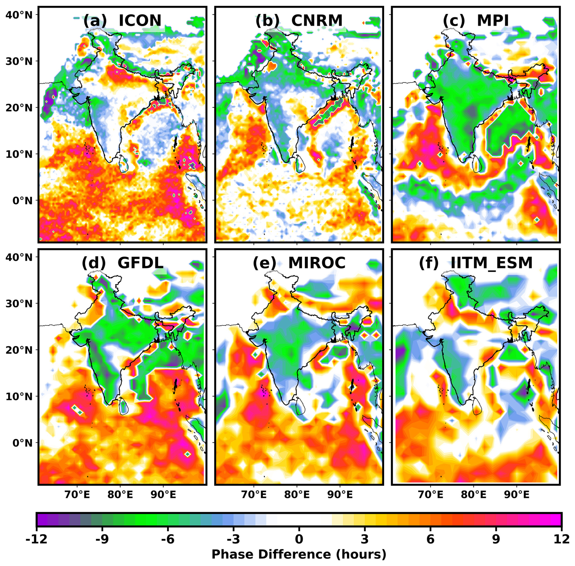
Figure 4 Climatological mean JJAS diurnal phase bias of precipitation (in hours) relative to IMERG from (a–f) ICON, CNRM, MPI, GFDL, MIROC, and IITM-ESM model simulations.

The combined amplitude and phase analyses indicate that ICON shows improved timing and intensity of diurnal rainfall compared to CMIP6 models, notable regional discrepancies persist, particularly over complex terrain and oceanic convection zones. To further examine the spatiotemporal structure of the diurnal signal, an EOF analysis is employed.

3.1.2 EOF analysis of diurnal rainfall

To identify dominant patterns of diurnal rainfall variability, we apply EOF analysis, which efficiently reduces the dimensionality of large datasets while retaining the key physical modes (Hannachi et al., 2007). EOFs are widely used in diurnal cycle studies as they capture coherent spatial–temporal structures that explain most of the observed variance. In high-resolution satellite data, the first two EOF modes typically account for over 80 %–90 % of the total variance (Lee and Wang, 2021). Higher-order modes generally correspond to semidiurnal oscillations (Kikuchi and Wang, 2008) and are not discussed here. Hence, our analysis focuses on the first two EOF modes to evaluate the ability of ICON and CMIP6 models to reproduce the principal diurnal rainfall regimes over the Indian monsoon region.

EOF1

The first EOF spatial mode (EOF1) in IMERG exhibits a pronounced land–ocean contrast, with positive loadings over most of the Indian landmass and negative loadings over adjacent oceanic regions, apart from a few regional exceptions (Fig. 5g). This bipolar structure represents the spatial signature of the diurnal harmonic and reflects differential surface heating arising from contrasting land–sea heat capacities. Such a land–sea contrast pattern is a robust feature of the atmospheric response to daily radiative forcing and has been consistently documented in earlier studies (Kikuchi and Wang, 2008; Lee and Wang, 2021). EOF1 explains approximately 64 % of the total variance, confirming its dominance in diurnal precipitation variability. Enhanced loadings along coastlines and elevated terrain – including the Himalayas, Western Ghats, and Arakan Yoma – indicate intensified diurnal convection linked to localized sea-breeze and valley-breeze convergence. The negative loadings over parts of the Himalayas reflect the nocturnal to early-morning rainfall peak (00:00–06:00 LST), nearly 12 h out of phase with the afternoon maximum over most of the Indian landmass.

The ICON model closely reproduces the observed EOF1 land–ocean contrast pattern (Fig. 5a), including the key regional features seen in IMERG (Fig. 5h), though with slightly weaker intensity over land. The negative loadings along the Himalayas appear broader and exhibit a modest southward displacement, and an additional weak negative center emerges along the eastern coastal landmass, which is absent in the IMERG pattern. Overall, ICON’s EOF1 accounts for 59 % of the total variance, approximately 5 % lower than IMERG, indicating a comparable but slightly weaker representation of the dominant diurnal mode. Among the CMIP6 models, several capture aspects of the land–sea contrast with varying fidelity. The high-resolution CNRM model most closely matches IMERG, both spatially and in variance explained (62 %), although the amplitude of loadings is substantially reduced (Fig. 5b). MPI model produces a stronger-than-observed bipolar contrast (Fig. 5c), explaining nearly 75 % of the variance around 9 % higher than IMERG. Despite its coarser resolution, MIROC realistically captures the spatial structure of the EOF1 mode (Fig. 5e), though with reduced variance (54 %). In contrast, GFDL and IITM-ESM fail to reproduce the characteristic land–ocean structure: GFDL exhibits predominantly negative loadings with weak contrast (Fig. 5d), while IITM-ESM shows widespread negative loadings over land and only weak positive signals over the peninsula.

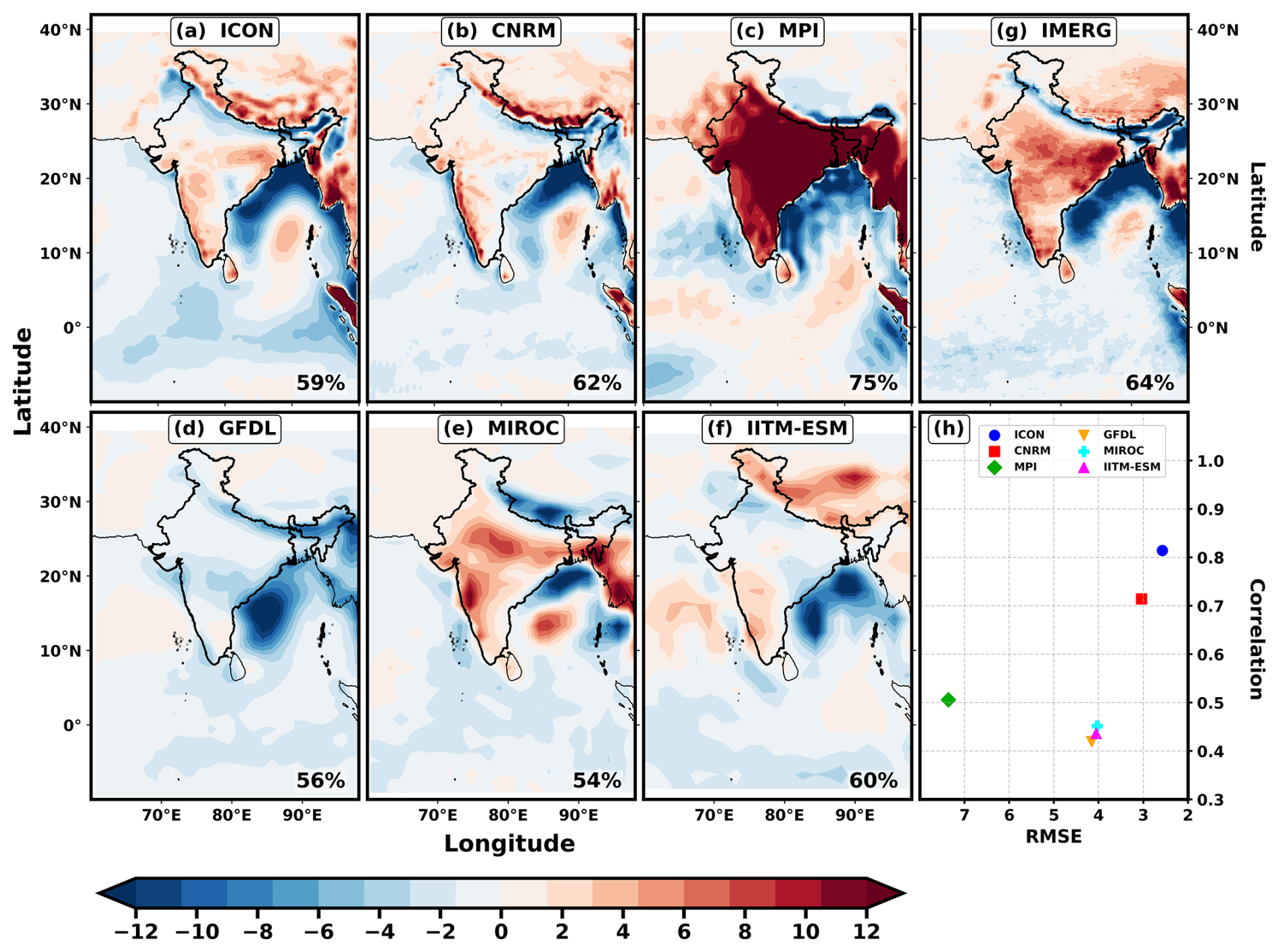
Figure 5 Spatial loading patterns of EOF1 for JJAS diurnal rainfall from (a–f) ICON, CNRM, MPI, GFDL, MIROC, and IITM-ESM model simulations, with (g) IMERG as the observational reference. Panel (h) shows the relationship between the spatial pattern correlation of EOF1 and the RMSE. The number in the lower right corner of each panel denotes the percentage of total variance explained by EOF1.

The comparative performance of these models is further quantified using the pattern correlation coefficient (PCC) and root-mean-square error (RMSE) of the EOF1 spatial distribution relative to IMERG. ICON shows the highest pattern correlation (PCC = 0.83) and lowest RMSE (2.3), followed by CNRM (PCC ≈ 0.7). GFDL, MIROC, and IITM-ESM exhibit comparable skill (PCC ≈ 0.42; RMSE ≈ 4.0). The MPI model, despite its strong spatial contrast, shows the largest RMSE (7) among all models, reflecting its tendency to overamplify the land–ocean gradient.

EOF2

The second EOF mode (EOF2) of diurnal precipitation is often termed as the Transition or the Coastal Mode. It represents the geographical variations that deviate from the universal land–sea contrast as captured by EOF1. While EOF1 explains the direct thermodynamic response to solar forcing, EOF2 classifies the complex diurnal regimes, associated with coastal propagation and topographic influences, including the relative strength of nighttime convection and phase propagation over complex terrain (Kikuchi and Wang, 2008).

In IMERG, EOF2 mode (Fig. 6g) displays distinct zonal and meridional gradients on either side of major coastal and orographic features and explains 27 % of the total variance. Positive loadings appear along the northern BoB and adjoining eastern coastal regions (northern Andhra Pradesh, Odisha, and West Bengal), while negative loadings dominate the southern Bay and southern east coast (southern Andhra Pradesh and Tamil Nadu). Over the Himalayan foothills, contrasting loadings emerge, with negative anomalies over the mountains and positive anomalies immediately southward, consistent with enhanced nocturnal convection in the plains and suppressed activity over elevated terrain. The peninsular interior is characterized largely by negative loadings. Among the models, the representation of this mode shows considerable diversity, reflecting the difficulty in simulating coastal and orographically triggered diurnal convection. The high-resolution models ICON and CNRM reproduce the broad spatial structure, but with some regional differences. ICON provides the closest match to IMERG, explaining 25 % of the total variance, while successfully capturing the alternating loadings along the eastern coastline. However, it reverses the sign of loadings over the Himalayas. CNRM similarly reproduces the eastern coastal features but fails to represent the Himalayan pattern. Among the coarser models, MIROC depicts the coastal–inland gradients reasonably well, while MPI shows partial agreement but with spatial artifacts. GFDL and IITM-ESM display distorted and weak loading structures, indicating limited fidelity. In terms of explained variance, GFDL (39 %), MIROC (35 %), and CNRM (31 %) overestimate the contribution of EOF2, whereas IITM-ESM (22 %) and MPI (17 %) underestimate it. Pattern statistics further distinguish model performance hierarchy with, ICON leading with highest correlation (PCC ≈ 0.6) and lowest RMSE (∼ 2.5 mm d⁻¹), followed by CNRM (PCC ≈ 0.5; RMSE ≈ 2.8 mm d⁻¹). MIROC and MPI show moderate correlation (PCC ≈ 0.4), though MPI retains larger error. GFDL exhibits negative correlation and the highest RMSE, indicating poor representation of this mode, while IITM-ESM, despite low PCC (∼ 0.2), captures some aspects of the propagating structure.

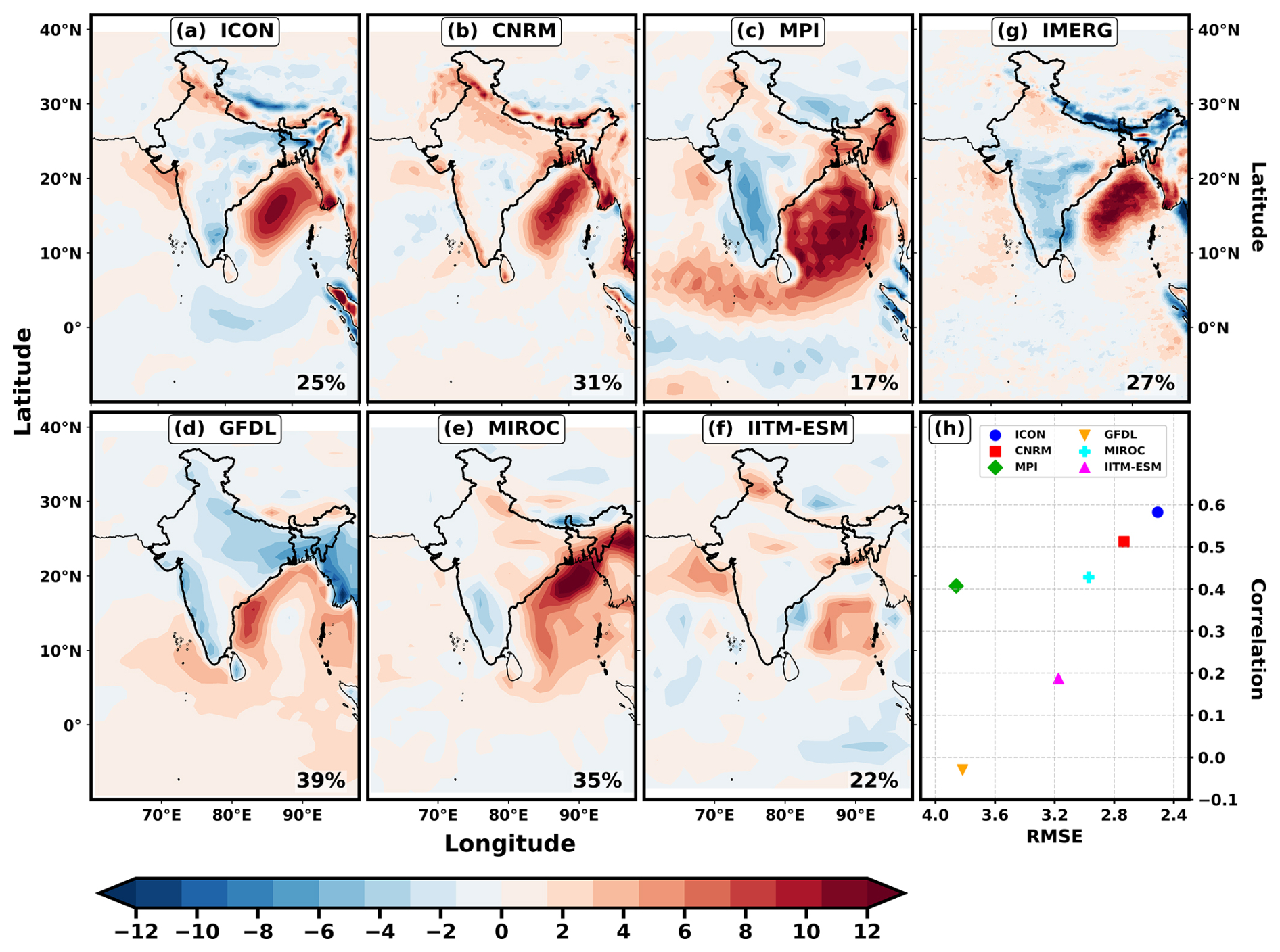
Figure 6 Same as Fig. 5, but for EOF2.

The spatial structure captured by EOF2 underscores the strong influence of coastal and orographic processes on the diurnal organization of rainfall, particularly between the eastern coastline and the BoB. However, the spatial loadings alone do not fully resolve the temporal evolution and migration characteristics embedded within this mode. To examine whether EOF2 represents organized eastward or coastal-propagating convection, a lead–lag regression analysis based on the EOF2 principal component (PC) is conducted in the following section.

To examine the propagation characteristics of diurnal convection, PC2 is regressed against diurnal rainfall anomalies with a ±15 h lead–lag over the latitudinal band 8–16° N, corresponding to the region of eastward-propagating convective systems from the Indian landmass into the BoB, as indicated by the EOF2 spatial pattern. In IMERG (Fig. 7g), a clear eastward propagation is evident. Positive anomalies appear near 80° E at lag −12 h and progressively shift eastward toward ∼ 90° E by lag +5 h, indicating a coherent propagating signal with an estimated phase speed of ∼ 16 m s⁻¹. The timing reflects afternoon convection over land followed by nighttime enhancement over the adjacent ocean, consistent with coastal propagation linked to land–sea-breeze circulations and mesoscale organization over the BoB (Kikuchi and Wang, 2008; Johnson, 2011). Such propagation is understood to arise from a combination of cold-pool-driven density currents, diurnally generated gravity waves, and land–sea thermal contrasts that modulate low-level convergence (Mapes et al., 2003; Yang and Slingo, 2001). Observational studies indicate that these signals typically travel at 8–15 m s⁻¹ over open ocean – faster than over land due to reduced surface drag – and can persist for several hundred kilometers, with the organized rainfall episode lasting longer than individual convective cells (Johnson, 2011).

ICON (Fig. 7a) reproduces the eastward-sloping regression structure and maintains a coherent propagating signal, though with slightly weaker amplitude and marginally faster phase speed than observed. CNRM captures the general eastward tilt but with reduced regression strength, indicating weaker coherence. In contrast, MPI, MIROC, and GFDL primarily exhibit standing or weakly evolving structures with limited longitudinal progression, while IITM-ESM shows low regression amplitude and poorly organized propagation. The relative regression magnitudes (Fig. 7h) further summarize these differences. IMERG exhibits the strongest signal (≈20), followed by ICON (≈15). Although MPI shows comparable amplitude, its pattern lacks clear propagation and is dominated by stationary features. The remaining models display weaker regression coefficients and limited temporal evolution, indicating difficulty in representing the propagating component of the diurnal cycle.

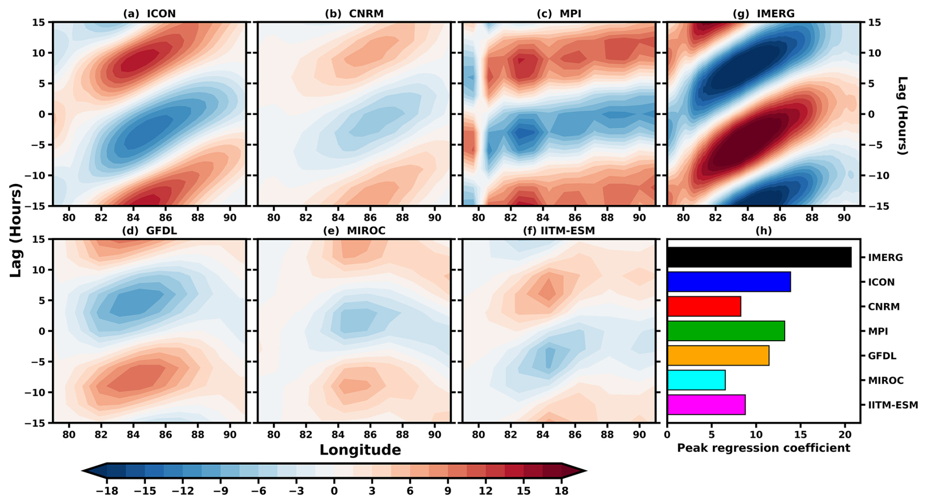
Figure 7 Eastward propagation of diurnal convective systems inferred from lead–lag regression (−15 to +15 h) between EOF2 principal component (PC2) and diurnal rainfall anomalies averaged over 8–16° N. Results are shown for (a–f) ICON, CNRM, MPI, GFDL, MIROC, and IITM-ESM, with (g) IMERG as the observational reference. Panel (h) summarizes the peak regression coefficients for IMERG and all models.

Overall, the lead–lag analysis demonstrates that simulating coastal diurnal propagation requires not only realistic amplitude but also coherent phase progression linked to mesoscale dynamics and land–ocean coupling processes. Differences across models suggest varying abilities to represent these interacting mechanisms.

The comprehensive diurnal-scale assessment indicates that, although several models capture aspects of convective timing, amplitude, and coastal propagation, systematic biases remain particularly over complex terrain and along land–sea transition zones. Errors in phase, amplitude, and mesoscale propagation at the diurnal scale are not isolated deficiencies; they can influence how convection organizes, aggregates, and interacts with larger-scale circulation. This multiscale interaction is corroborated by recent observational evidence demonstrating that the diurnal amplitude of precipitation is actively amplified or suppressed during the wet and dry spells of high- and low-frequency ISOs, respectively (Misra and Jayasankar, 2026). Such biases may subsequently affect the representation of synoptic disturbances, ISOs, and ultimately the seasonal mean monsoon rainfall. To evaluate whether these scale-dependent errors persist or amplify across temporal hierarchies, the following sections examine model performance at synoptic (3–7 d), intraseasonal (10–90 d), and seasonal (> 90 d) timescales.

3.2 Monsoon variability in other scales (Synoptic, intraseasonal, and seasonal)

3.2.1 Power Spectrum

The power spectral density (PSD) of daily rainfall quantifies the distribution of variance across temporal frequencies and provides insight into the temporal organization of monsoon convection (Torrence and Compo, 1998; Wheeler and Kiladis, 1999). Over CI, the IMERG spectrum (Fig. 8g) exhibits well-defined peaks in three characteristic bands: synoptic disturbances (2–7 d), higher-frequency intraseasonal variability (10–20 d), and lower-frequency ISOs (30–60 d), consistent with established characterizations of monsoon variability (Goswami et al., 2006; Saha et al., 2014). The dominant peak occurs near 5.3 d with maximum power of ∼ 18 mm² d⁻² (Fig. 8h), and the spectrum displays the expected red-noise decay toward higher frequencies.

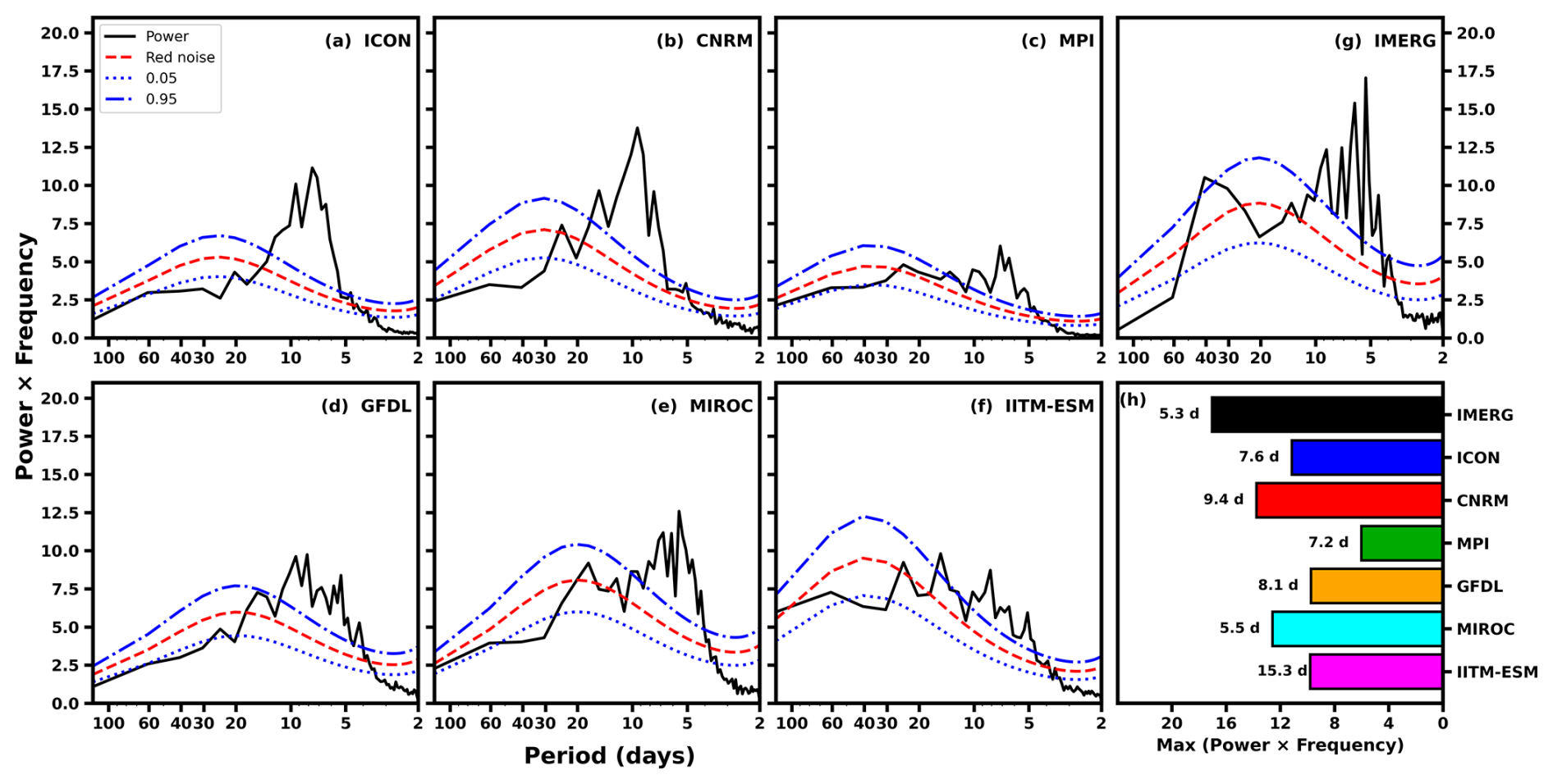
Figure 8 Composite power spectra of JJAS mean daily rainfall anomalies averaged over Indian region 10–25° N, 80–100° E (box ref: Saha et al., 2014) from (a–f) ICON, CNRM, MPI, GFDL, MIROC, and IITM-ESM, with (g) IMERG as observational references. The dashed blue curves denote the 5 % and 95 % confidence levels, and the red dashed curve represents the theoretical red-noise spectrum. Panel (h) summarizes the dominant period and corresponding peak spectral power for IMERG and all models.

ICON (Fig. 8a) reproduces the overall spectral shape and retains a dominant synoptic-scale peak at 7.6 d, though with reduced amplitude (∼ 12–13 mm² d⁻²). A secondary signal appears in the 10–20 d band, marginally above the red-noise background, while the 30–60 d band is substantially underestimated. Thus, although the hierarchical structure of variability is maintained, intraseasonal power remains weakened. CNRM (Fig. 8b) shifts its dominant peak toward the 10–20 d band (∼ 9.4 d), producing one of the higher peak amplitudes among the models (∼ 14 mm² d⁻²), but with comparatively weak synoptic and lower frequency intraseasonal variance. MPI (Fig. 8c) exhibits the lowest overall spectral energy – approximately one-third of IMERG – with its maximum centered ∼ 7.2 d (∼ 6 mm² d⁻²), indicating muted variability across all timescales. Among the coarser-resolution models, MIROC (Fig. 8e) most closely matches the observed dominant period (5.5 d) and produces a reasonable peak amplitude (∼ 14 mm² d⁻²), though intraseasonal power remains underestimated. GFDL (Fig. 8d) retains synoptic-band dominance (∼ 8.1 d) but with weaker amplitude. In contrast, IITM-ESM (Fig. 8f) shifts its primary peak into the 10–20 d band (∼ 15.3 d), with moderate amplitude but limited synoptic-scale variance.

A consistent feature across all simulations is the marked underestimation of lower frequency intraseasonal (30–60 d) variability. Such weakening is commonly reported in AMIP-type integrations, where prescribed monthly SSTs limit two-way ocean–atmosphere feedbacks that are essential for sustaining coupled ISOs (Waliser et al., 2003; Jiang et al., 2020). Reduced synoptic-band power in several models further suggests limited representation of organized MCSs, which contribute substantially to rainfall variance at these periods. Overall, while several models reproduce the broad spectral hierarchy of monsoon rainfall, systematic reductions in variance – particularly in the intraseasonal bands – remain evident. These scale-dependent differences in spectral power provide a dynamical context for the amplitude biases identified earlier and motivate further examination of rainfall intensity distributions.

To complement the spectral analysis, we examine the probability density function (PDF) of daily rainfall to assess how differences in temporal variability translate into biases in rainfall intensity and frequency across models.

3.2.2 Probability Density Function (PDF)

The PDF analysis was performed over the CI region using each model’s native grid resolution. The PDF values were normalized by the total number of grid points within each rainfall bin, ensuring a consistent statistical comparison across models and observations. Figure 9 is divided into three panels: the main panel displays rainfall intensities between 0 and 20 mm d⁻¹, while the two inset panels extend the range to 20–60 and 60–100 mm d⁻¹, respectively.

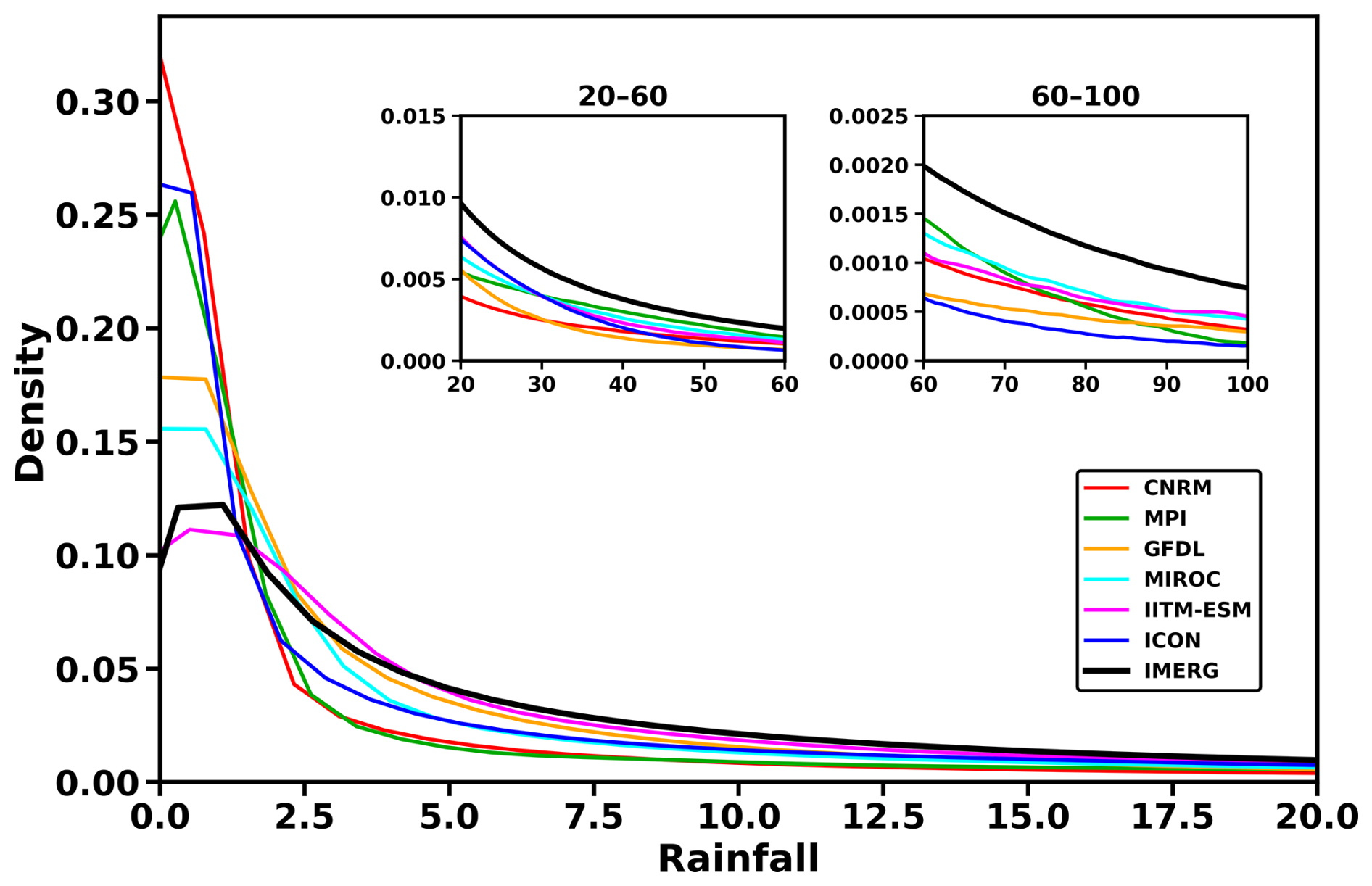
Figure 9 Probability density function (PDF) of JJAS daily rainfall over Central India from ICON and CMIP6 models (CNRM, MPI, GFDL, MIROC, and IITM-ESM), compared with IMERG on each dataset's native grid. The main panel shows 0–20 mm d⁻¹, with inset panels extending to 20–60 and 60–100 mm d⁻¹.

A common feature across most models is an enhanced frequency of light rainfall events (0–2 mm d⁻¹) relative to IMERG, indicative of the well-documented “drizzle bias” associated with parameterized convection (Chen et al., 2021; Dai, 2006; Stephens et al., 2010), although observational uncertainties in light rainfall retrievals remain (Prakash and Srinivasan, 2021). The higher-resolution models (ICON, CNRM, and MPI) exhibit particularly elevated occurrence of weak precipitation, suggesting frequent triggering of shallow or weakly organized convection. In contrast, the coarser-resolution models (GFDL and MIROC) show comparatively reduced drizzle frequency, while IITM-ESM (≈ 190 km) slightly underestimates light rainfall and aligns more closely with IMERG in this narrow range. Beyond light intensities, systematic underestimation of moderate-to-heavy rainfall becomes evident across nearly all models. IMERG consistently shows higher probability across the 5–100 mm d⁻¹ range, underscoring a general model tendency to underrepresent organized and intense convective events. Between 5 and 30 mm d⁻¹, ICON produces higher occurrence than CNRM and MPI but lower than GFDL and MIROC. In the 20–30 mm d⁻¹ range, ICON shows the largest frequency among the higher-resolution models, though its distribution declines rapidly beyond 30 mm d⁻¹. MPI exhibits comparatively larger frequency in the 30–70 mm d⁻¹ range, whereas MIROC extends the heavy-rainfall tail into the 70–100 mm d⁻¹ band, though with lower overall probability than IMERG. Across the 2.5–15 mm d⁻¹ range, coarser models dominate, reflecting a shift of rainfall occurrence toward moderate intensities. Since rainfall PDFs are sensitive to grid spacing, the analysis is repeated after regridding IMERG and all model outputs to a common grid corresponding to the IITM-ESM resolution of approximately 1.9° (Fig. S2). The common-grid comparison modifies the rainfall distributions, particularly at light and moderate intensities, confirming that part of the native-grid behaviour is resolution dependent. After regridding, the frequency of moderate rainfall becomes closer to IMERG in several models, while all models continue to underestimate the heavy-rainfall tail in the 60–100 mm d⁻¹ range. Thus, the common-grid analysis supports a more resolution-consistent comparison, whereas the native-grid PDFs retain information on how each model configuration represents rainfall at its own effective resolution.

These resolution-dependent differences likely arise from contrasting representations of convective organization and grid-scale averaging. At higher resolutions, increased triggering of parameterized convection can lead to frequent but weak rainfall events, thereby enhancing light-rain probabilities while limiting moisture buildup required for intense precipitation (Dai, 2006; Stephens et al., 2010). Conversely, coarse grids spatially smooth rainfall and may artificially aggregate convective activity into moderate intensities, while still underrepresenting extreme events due to limited representation of mesoscale convective systems (MCSs) and subgrid variability (Kendon et al., 2012; Prein et al., 2015). Additionally, the inability of parameterized convection to capture cold-pool dynamics, slantwise overturning circulations within organized MCSs (Moncrieff, 2019), and upscale growth of convective systems can suppress the heavy-rainfall tail across models.

Overall, the native- and common-grid PDFs indicate a systematic redistribution of rainfall toward light-to-moderate intensities and a consistent underrepresentation of heavy rainfall events. The comparison also shows that rainfall-intensity distributions are resolution sensitive, particularly at light and moderate intensities, but important inter-model differences remain even after regridding to a common resolution. When viewed alongside the spectral analysis, these distributional biases reinforce the conclusion that deficiencies in convective parameterization and mesoscale organization affect both the temporal variance and intensity structure of monsoon rainfall. Such biases at daily scales may propagate upward, influencing synoptic aggregation and intraseasonal variability.

3.2.3 Rainfall Variance

The spatial distribution of band-pass filtered rainfall variance in the synoptic (2–7 d) and intraseasonal (10–20 and 20–100 d) bands delineates the regions where these modes are most active and provides insight into the underlying dynamical processes that organize monsoon rainfall. Together, these three frequency bands account for the bulk of the seasonal variability of the Indian Summer Monsoon Rainfall (ISMR), as demonstrated by Saha et al. (2014). Figure 10 presents the variance computed from filtered daily rainfall anomalies across these bands, while Fig. S3 complements the spatial analysis by summarizing the PCC and RMSE of each model relative to IMERG, thereby enabling a quantitative evaluation of model skill across temporal scales.

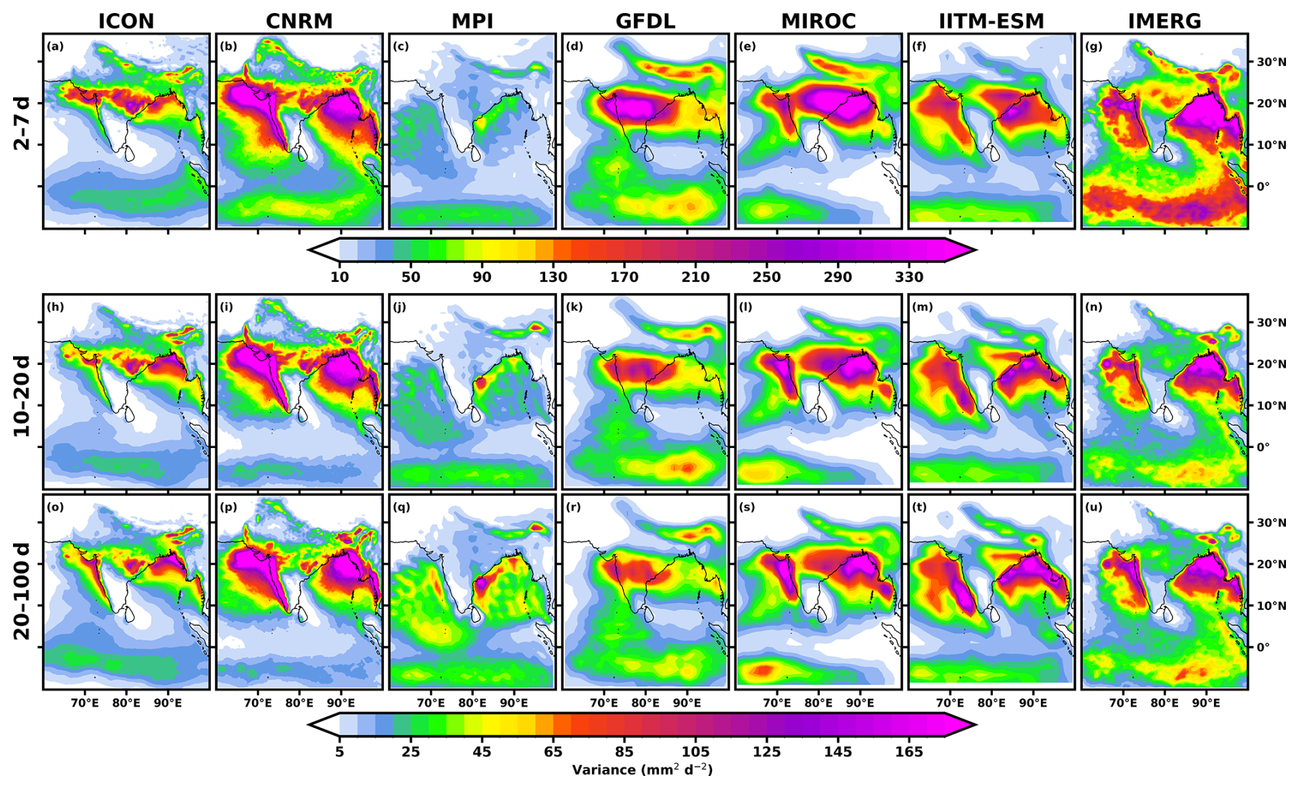
Figure 10 Climatological JJAS rainfall variance in synoptic (2–7 d), higher frequency ISO (10–20 d) and lower frequency ISO (20–100 d) band using filtered daily rainfall anomaly (in mm² d⁻²) from ICON, all the participant CMIP6 (CNRM, MPI, GFDL, MIROC, and IITM-ESM) model simulations, and IMERG as observational reference.

In IMERG (Fig. 10g), the synoptic band accounts for the largest share of seasonal variance (∼ 190 mm² d⁻²), with pronounced maxima along the climatological monsoon trough extending from CI to the head BoB, and secondary centres over the Arabian Sea and Himalayan foothills. This distribution reflects the genesis and westward propagation of monsoon lows and depressions embedded within the trough circulation, as well as terrain-modulated convection along the Western Ghats and Himalayan foothills (e.g. Goswami et al., 2003). The enhanced synoptic variance over the eastern equatorial Indian Ocean likely arises from convectively coupled equatorial wave activity and its interaction with the background monsoon flow, which organizes convection at 2–7 d timescales and contributes to the initiation of larger-scale variability. At intraseasonal timescales, the 10–20 (Fig. 10n) and 20–100 (Fig. 10u) day bands exhibit broadly similar spatial structures, highlighting the multiscale envelope of monsoon variability. Variance maxima remain anchored along the monsoon trough and the head BoB, while the equatorial Indian Ocean emerges as a key centre, particularly in the 20–100 d band consistent with the genesis region of the monsoon intraseasonal oscillation (MISO), which subsequently propagates northward over the subcontinent (e.g. Sikka, 1977; Saha et al., 2014). The enhancement of variance over the equatorial Indian Ocean at 20–100 d underscores the coupled ocean–atmosphere processes central to large-scale intraseasonal organization.

Across models, the gross spatial organization is reproduced, but amplitude and regional fidelity vary. In the synoptic band, both IITM-ESM and CNRM shows the highest spatial agreement with IMERG (PCC ≈ 0.66 and 0.65 respectively) and lowest RMSE (∼ 80 mm² d⁻²) among other models. They are closely followed by MIROC (PCC ≈ 0.58; RMSE ≈ 90 mm² d⁻²). ICON captures the correct trough-aligned structure but with moderate amplitude underestimation, especially over oceanic and orographic regions (PCC ≈ 0.56; RMSE ≈ 130 mm² d⁻²). MPI substantially underestimates variance and misrepresents the trough orientation, while GFDL reproduce the large-scale structure but show moderate displacement of oceanic maxima. Consistent with observation, most models exhibit broadly similar spatial variance distributions in the 10–20 and 20–100 d bands. The primary distinction emerges over the equatorial Indian Ocean, where variance intensifies in the 20–100 d band, consistent with the genesis region of the MISO. An exception is MPI, which produces unrealistically large 20–100 d variance across all ocean basins (Arabian Sea, Bay of Bengal, and equatorial Indian Ocean), suggesting an over-amplified low-frequency oceanic signal. In the 10–20 d band, MIROC exhibits the highest spatial fidelity (PCC ≈ 0.78), followed by ICON and IITM-ESM (PCC ≈ 0.74). In terms of RMSE, the coarser-resolution models (e.g. MIROC and IITM-ESM) show smaller errors, with RMSE values (∼ 20 mm² d⁻²) nearly half of ICON's, primarily due to ICON’s underestimation of oceanic variance. In the 20–100 d band, MIROC again attains the highest PCC (∼ 0.80), followed by ICON (∼ 0.78) and then by IITM-ESM and CNRM (∼ 0.70). Here too higher resolution model (ICON and CNRM) has higher RMSE (∼ 42 mm² d⁻²). The higher RMSE in ICON is consistent with its enhanced variance in the intraseasonal band, as also noted by Pothapakula et al. (2026), who reported higher variability across multiple resolutions (10, 40, and 80 km) over the CI region. The remaining models cluster at substantially lower correlations and higher errors, indicating weaker spatial fidelity and amplitude biases in representing intraseasonal variability.

Synoptic-scale variance is most realistically represented by IITM-ESM and CNRM, whereas MIROC consistently leads in both intraseasonal bands, with ICON performing competitively and IITM-ESM slightly behind at longer timescales. Although most models reproduce the broad spatial organization of multiscale variance, systematic amplitude biases persist, especially over the equatorial Indian Ocean and monsoon trough core regions. These discrepancies underscore ongoing challenges in representing the dynamical coupling between monsoon depressions, ocean–atmosphere feedbacks, and large-scale intraseasonal convection, highlighting the importance of accurately simulating multiscale interactions within the monsoon system.

3.2.4 Rainfall seasonal mean

The seasonal mean rainfall represents the combined effect of processes across shorter timescales from diurnal convection to synoptic systems and ISOs, thereby representing the cumulative outcome of all mechanisms that shape monsoon rainfall. Thus, the seasonal mean serves as an integrated test of model performance, indicating whether skill at shorter timescales translates into realistic seasonal accumulation or whether multiscale biases amplify into systematic errors.

In IMERG (Fig. 11g), the seasonal rainfall pattern aligns closely with the previously identified variance hotspots. Regions characterized by strong synoptic activity and terrain-modulated convection – such as the monsoon trough corridor and major orographic belts – emerge as the principal rainfall maxima. Likewise, the equatorial Indian Ocean, highlighted earlier as a center of intraseasonal variance and MISO genesis (e.g. Yasunari, 1979; Saha et al., 2014), contributes substantially to seasonal accumulation through persistent large-scale convergence and low-frequency modulation. Thus, the climatological mean reflects the spatial imprint of multiscale convective organization rather than independent large-scale forcing alone.

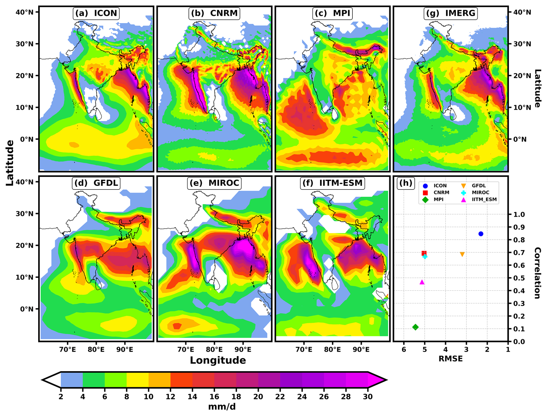
Figure 11 Seasonal (JJAS) averaged climatological mean rainfall (in mm d⁻¹) from (a) ICON, all the participant CMIP6 (b–f: CNRM, MPI, GFDL, MIROC, and IITM-ESM) model simulations, and IMERG (g) as observational reference. Panel (h) shows the scatter between pattern correlation and RMSE.

Model performance at the seasonal scale largely reflects their variance characteristics, while the bias patterns (Fig. S4) clarify how systematic biases accumulate spatially. ICON (Fig. 11a) maintains strong spatial coherence with IMERG (PCC = 0.85; RMSE = 2.3 mm d⁻¹), indicating that its relatively balanced representation of synoptic and intraseasonal variability translates into a realistic seasonal rainfall structure. Its bias field exhibits a weak dipole over land, with alternating wet and dry anomalies across central and peninsular India, while oceanic deviations remain modest (generally within ±3 mm d⁻¹). The limited amplitude of these biases suggests that residual multiscale errors are not strongly amplified in the seasonal integration.

CNRM (Fig. 11b) shows reasonable spatial alignment (PCC ≈ 0.65–0.70; RMSE ≈ 5 mm d⁻¹) but overestimates rainfall along the Western Ghats and parts of the monsoon trough while underestimating over sections of the equatorial Indian Ocean, consistent with its enhanced land-based variance and comparatively weaker low-frequency oceanic variability. MPI (Fig. 11c) displays weak spatial skill (PCC ≈ 0.1; RMSE ≈ 5.5 mm d⁻¹), with widespread oceanic wet biases and dry bias over monsoon trough region, reflecting its excessive low-frequency oceanic variance.

Among the coarser-resolution models, GFDL and MIROC (Fig. 11d, e) display contrasting but systematic bias signatures. GFDL (PCC ≈ 0.65–0.70; RMSE ≈ 3.2 mm d⁻¹) shows a dry bias along the monsoon trough and head BoB but wet anomalies over the Arabian Sea and southern BoB. MIROC, while capturing the broad monsoon envelope, exhibits pronounced wet biases over the Arabian Sea and BoB and a substantial dry bias over the eastern equatorial Indian Ocean, contributing to higher RMSE. These opposing tendencies are consistent with their differing representations of oceanic variance amplitude identified in the previous section. However, IITM-ESM (Fig. 11f) occupies an intermediate position, with alternating wet and dry anomalies along the trough and a marked wet bias over the Arabian Sea coupled with dry conditions over the equatorial Indian Ocean, indicating persistent land–ocean amplitude imbalance despite good synoptic variance skill.

Overall, the seasonal climatology reinforces the multiscale diagnostics: models that more realistically represent synoptic and intraseasonal organization tend to better reproduce the integrated monsoon rainfall pattern. However, systematic oceanic overestimation and regional amplitude biases demonstrate that variance errors do not average out but project coherently onto the seasonal mean. Accurate simulation of ISMR therefore depends critically on balanced cross-scale interactions rather than correct seasonal circulation alone.

3.2.5 Annual Rainfall

The seasonal mean rainfall highlighted the accumulated imprint of multiscale variability and the annual cycle, in contrast, reveals its temporal evolution. By tracing the onset, northward migration, peak, and withdrawal of the monsoon rainband, it provides a dynamic view of how the seasonal state develops. Here we discuss the latitude–time evolution over 70–90° E, enabling assessment of each model’s ability to capture the timing, amplitude, and meridional progression of monsoon rainfall. Most models capture this northward migration pattern with varying degrees of accuracy. Earlier model generations often failed to simulate this evolution realistically (e.g. Pokhrel et al., 2018a).

IMERG (Fig. 12g) clearly captures three distinct rainfall regimes: equatorial precipitation maxima during the pre-monsoon (April–May) and post-monsoon (October–November) seasons, and a pronounced northward migration of convection reaching 25° N during JJAS. This meridional shift reflects the seasonal transition from the OTCZ to the Continental Tropical Convergence Zone (CTCZ), a defining characteristic of the dynamical large-scale monsoon system and closely linked to monsoon intraseasonal variability. The latitude of maximum rainfall (shown in a overlaid black line) remains anchored over the Indian mainland throughout JJAS before retreating southward in September, marking the observed withdrawal phase.

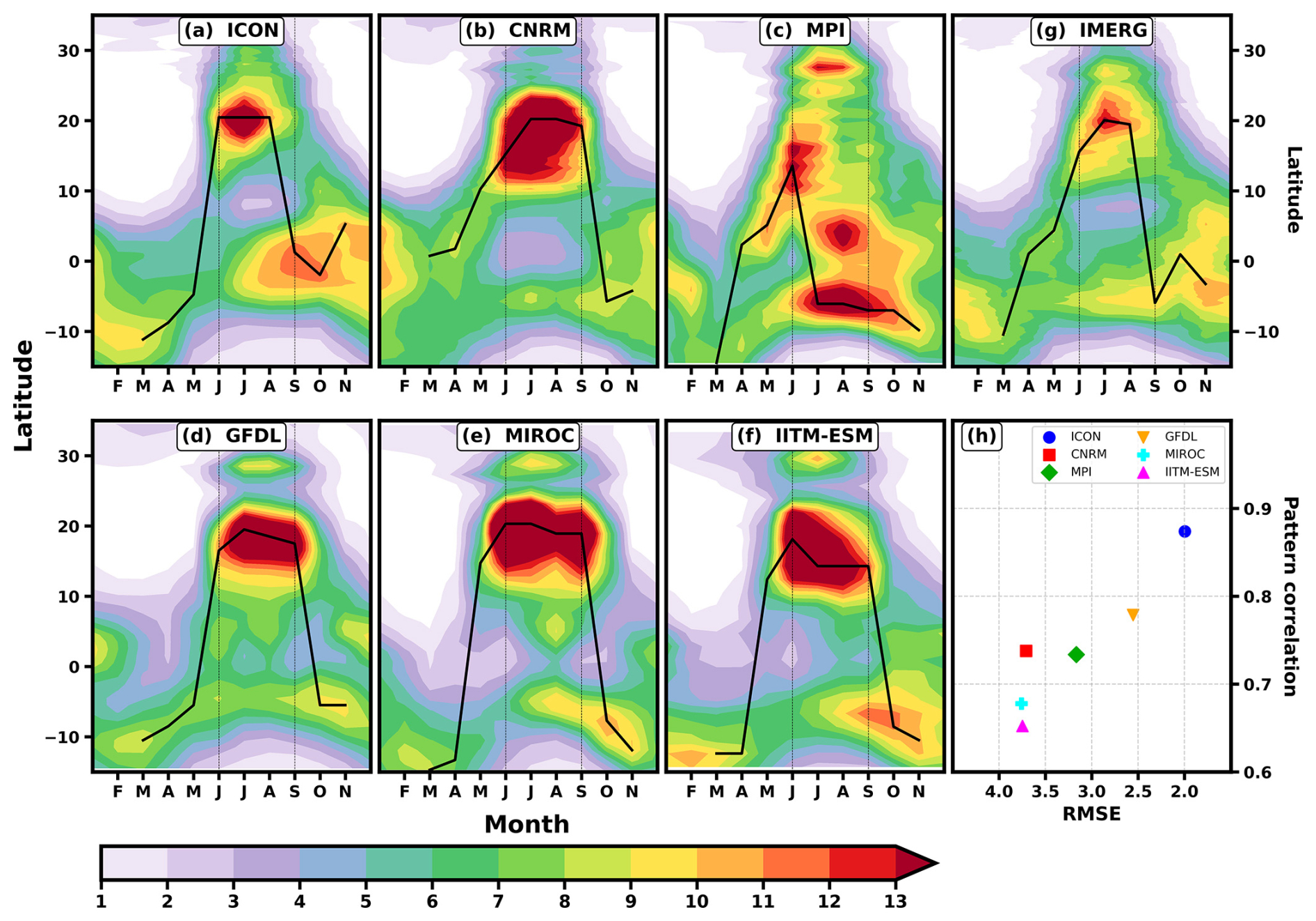
Figure 12 Latitude–time evolution of the climatological mean annual cycle of precipitation (mm d⁻¹) averaged zonally over the Indian monsoon region (70–90°E) from (a–f) ICON, CNRM, MPI, GFDL, MIROC, and IITM-ESM model simulations, with (g) IMERG as observational reference. The overlaid black curve denotes the latitude of maximum precipitation, illustrating the seasonal migration of the monsoon rainband. The faint black dotted lines mark the monsoon season (JJAS). Panel (h) presents the scatter of pattern correlation coefficient (PCC) versus root-mean-square error (RMSE) for all models relative to IMERG.

Most models reproduce the broad northward migration, though with systematic differences in amplitude and timing. Earlier model generations often struggled to simulate this seasonal evolution realistically (e.g. Pokhrel et al., 2018a), but several CMIP6 models and ICON show notable improvement in capturing the transition between oceanic and continental convection. ICON most faithfully reproduces both the seasonal progression and the September withdrawal, consistent with IMERG. In contrast, MPI allows rainfall to extend north of 25° N but retains its core maximum near 15° N, indicating weaker continental convection and excessive OTCZ rainfall; its withdrawal occurs prematurely around July. CNRM, GFDL, MIROC, and IITM-ESM generally overestimate rainfall within the CTCZ while underestimating OTCZ intensity, and most simulate a delayed retreat in October rather than September. Quantitatively, the PCC–RMSE analysis (Fig. 12h) confirms ICON's superior performance (PCC = 0.88; RMSE = 2.0 mm d⁻¹), followed by GFDL (PCC = 0.78; RMSE = 2.5 mm d⁻¹), while the remaining models cluster within PCC = 0.65–0.74 and RMSE = 3.2–3.9 mm d⁻¹.

To further assess seasonal phase evolution, the domain-averaged annual cycle over the Indian land region is examined (Fig. S5). Over land, all models reproduce the observed unimodal structure. ICON and GFDL best simulate onset and peak timing during July–August; however, ICON shows slightly early withdrawal, whereas GFDL exhibits a broader seasonal extent with delayed retreat. MPI closely follows in structure but underestimates peak intensity. CNRM and MIROC overestimate peak rainfall, while IITM-ESM substantially underestimates it. The Taylor diagram (Fig. S5d) reflects this hierarchy: ICON, GFDL, and MPI cluster with 0.99 correlation and realistic variance, whereas MIROC and CNRM overestimate variance by 20 %–30 %, and IITM-ESM underestimates it by 20 %.

Over the extended monsoon region – including adjacent oceanic areas – all models tend to produce higher rainfall than IMERG observations (Fig. S5a). MPI exhibits the largest positive bias, driven by excessive oceanic rainfall despite weaker land precipitation. GFDL shows a wet bias extending beyond September, consistent with its delayed withdrawal. Most models display a broader seasonal distribution than observed, suggesting early onset and/or late retreat tendencies. ICON again remains closest to observations, capturing both seasonal progression and peak intensity. This is corroborated by the Taylor plot (Fig. S5c), where ICON shows 0.99 correlation and accurately reproduces observed variance, closely followed by GFDL (correlation = 0.98). CNRM slightly overestimates variance (correlation = 0.91), while IITM-ESM, MPI, and MIROC overestimate variance by approximately 30 %, 45 %, and 50 %, respectively, despite relatively high correlations (0.96–0.98).

Thus, the annual cycle analysis confirms that a multiscale perspective is essential for interpreting monsoon simulation fidelity. Models that maintain a balanced multiscale variance structure and weaker cross-scale error coupling tend to exhibit improved seasonal migration and annual-cycle fidelity, as further supported by the scale-wise and cross-scale diagnostics discussed in Sect. 3.3. In contrast, models with strongly coupled synoptic and intraseasonal bias structures often show larger seasonal-scale deviations, including premature retreat, broadened seasonal extent, or exaggerated peak intensity. These results show that realistic monsoon simulation depends on consistent cross-scale organization, as errors in variability do not disappear through seasonal averaging but instead project directly onto the evolving seasonal structure.

3.3 Multiscale Rainfall Biases

Do the systematic rainfall biases identified at individual timescales translate into scale-dependent variance biases relative to IMERG? Moreover, does such redistribution differ between land and ocean, where distinct dynamical controls operate? To address these questions, this section examines how models redistribute monsoon variability from higher to lower frequencies using area-averaged diagnostics over two representative regions, CI and the BoB (as shown in Fig. 13f), capturing the contrasting continental and oceanic regimes.

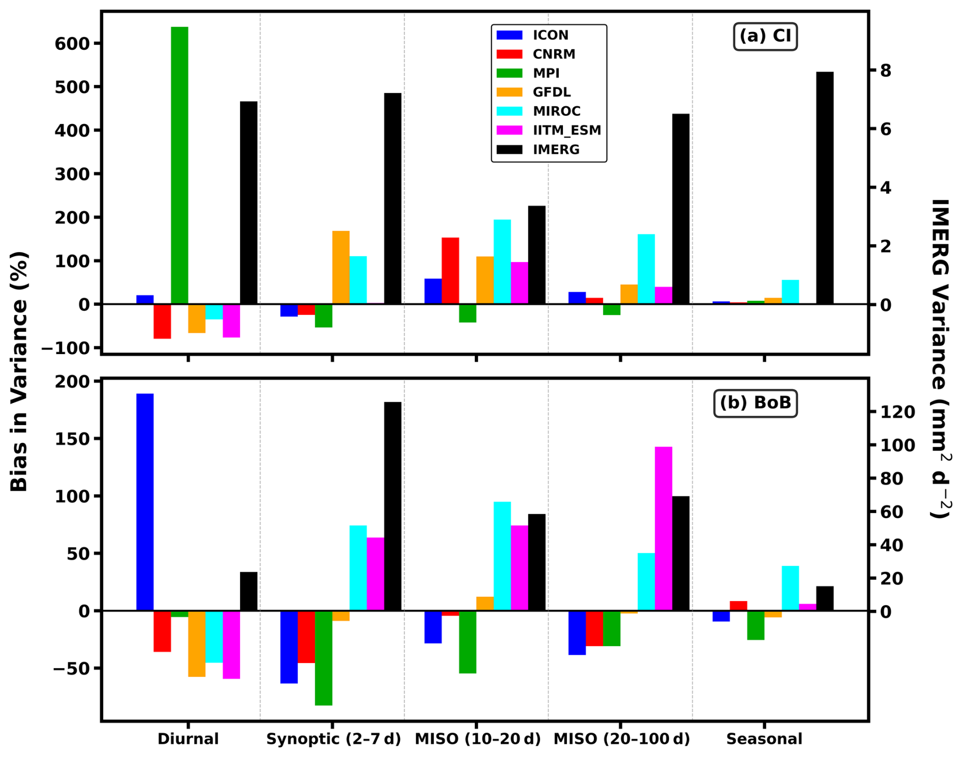
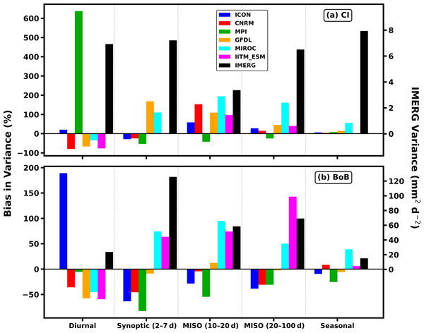
Figure 13 Percentage climatological JJAS rainfall variance bias relative to IMERG, computed as $\left[\left({\mathit{\sigma }}_{\mathrm{model}}^{\mathrm{2}}-{\mathit{\sigma }}_{\mathrm{IMERG}}^{\mathrm{2}}\right)/{\mathit{\sigma }}_{\mathrm{IMERG}}^{\mathrm{2}}\right]\times \mathrm{100}$, for the diurnal, synoptic, higher frequency MISO (10–20 d), lower frequency MISO (20–100 d), and seasonal (JJAS) bands. Results are shown for ICON and CMIP6 AMIP models (CNRM, MPI, GFDL, MIROC, and IITM-ESM) over (a) Central India (CI) and (b) Bay of Bengal (BoB) region. The analysis domains are indicated in Fig. 2.

Over CI, variance biases shows how the models redistribute their continental convective variability across scales. ICON maintains the most balanced structure, with deviations largely within ±50 %, slightly underestimating synoptic variance while modestly enhancing intraseasonal variability. This aligns with earlier findings that it captures the spatial organization of monsoon LPS but underestimates their intensity (e.g. Deoras et al., 2021).

MPI, in contrast, shows extreme amplification of diurnal variance (> 600 %), corresponding to an excess of ∼ 48 mm² d⁻² relative to the observed ∼ 8 mm² d⁻², as also seen in Fig. 2 where it showed the largest diurnal amplitude bias among all models. This behaviour is consistent with excessive high-frequency convection and the well-known “drizzling bias” in global models (Dai, 2006; Zhou et al., 2008; Chen et al., 2021), often linked to premature triggering of deep convection during boundary-layer growth over heated land surfaces. Notably, although both MPI and ICON employ mass-flux-based convective parameterizations, their diurnal biases differ markedly. MPI strongly overestimates land diurnal variance, whereas ICON remains comparatively controlled over land. This contrast suggests that diurnal variance errors arise not from the parameterization framework alone, but from how it interacts with land–atmosphere coupling processes. Most other models, meanwhile, suppress diurnal variance over land, indicating weakened high-frequency convective organization. At synoptic and intraseasonal scales, GFDL and MIROC tend to amplify organized variability, whereas IITM-ESM exhibit more moderate, scale-dependent biases.

Thus, over land, inter-model divergence primarily reflects how energy is partitioned between diurnal convection and organized synoptic–intraseasonal disturbances, shaping the seasonal rainfall structure discussed earlier.

Over the BoB, the bias structure shifts, underscoring the dominant role of ocean–atmosphere interaction. ICON exhibits a pronounced positive diurnal variance bias (∼ 180 %, ∼ 54 mm² d⁻² relative to the observed ∼ 30 mm² d⁻²), consistent with its enhanced oceanic diurnal amplitude noted previously. Unlike over land, this amplification likely reflects an over-responsive coupling of convection to low-level moisture convergence under prescribed SST conditions. In strongly coupled oceanic regions such as the BoB, the absence of two-way air–sea feedback in AMIP simulations can exaggerate atmospheric variability (Pegion and Kirtman, 2008; DeMott et al., 2014). At synoptic and intraseasonal scales, ICON’s biases turn negative but remain within ±60 %, indicating relatively realistic organized variability despite enhanced high-frequency convection. Among CMIP6 models, IITM-ESM shows the strongest amplification at lower frequencies, with ∼ 100 % positive bias in the 20–100 d band (an excess of ∼ 160 mm² d⁻² relative to the observed ∼ 80 mm² d⁻²), followed by ∼ 60 % in the 10–20 d band and ∼ 40 % in the synoptic band, while suppressing diurnal variance (∼ 50 %). MIROC exhibits a similar but slightly weaker enhancement of intraseasonal variance (∼ 80 % in 10–20 d and ∼ 50 % in synoptic bands). In contrast, MPI and CNRM generally suppress synoptic and intraseasonal variability over the ocean, while GFDL remains comparatively balanced, with most biases within ±10 % except for a ∼ 50 % reduction in diurnal variance.

The land–ocean contrast is therefore clear: over land, variance biases are dominated by errors in diurnal–synoptic partitioning and boundary-layer convection coupling, whereas over the ocean, biases primarily reflect misrepresentation of intraseasonal modulation and air–sea interaction. These systematic variance imbalances set the stage for the amplitude biases in the phase-locked diurnal and seasonal cycles discussed next.

Figure 14 isolates rainfall amplitude biases at the two phase-locked endpoints of the temporal spectrum – diurnal and seasonal scales – thereby complementing the variance redistribution diagnosed in Fig. 13. Because these scales are locked to the diurnal and annual cycles, respectively, amplitude biases provide a direct measure of systematic intensity errors rather than variability redistribution.

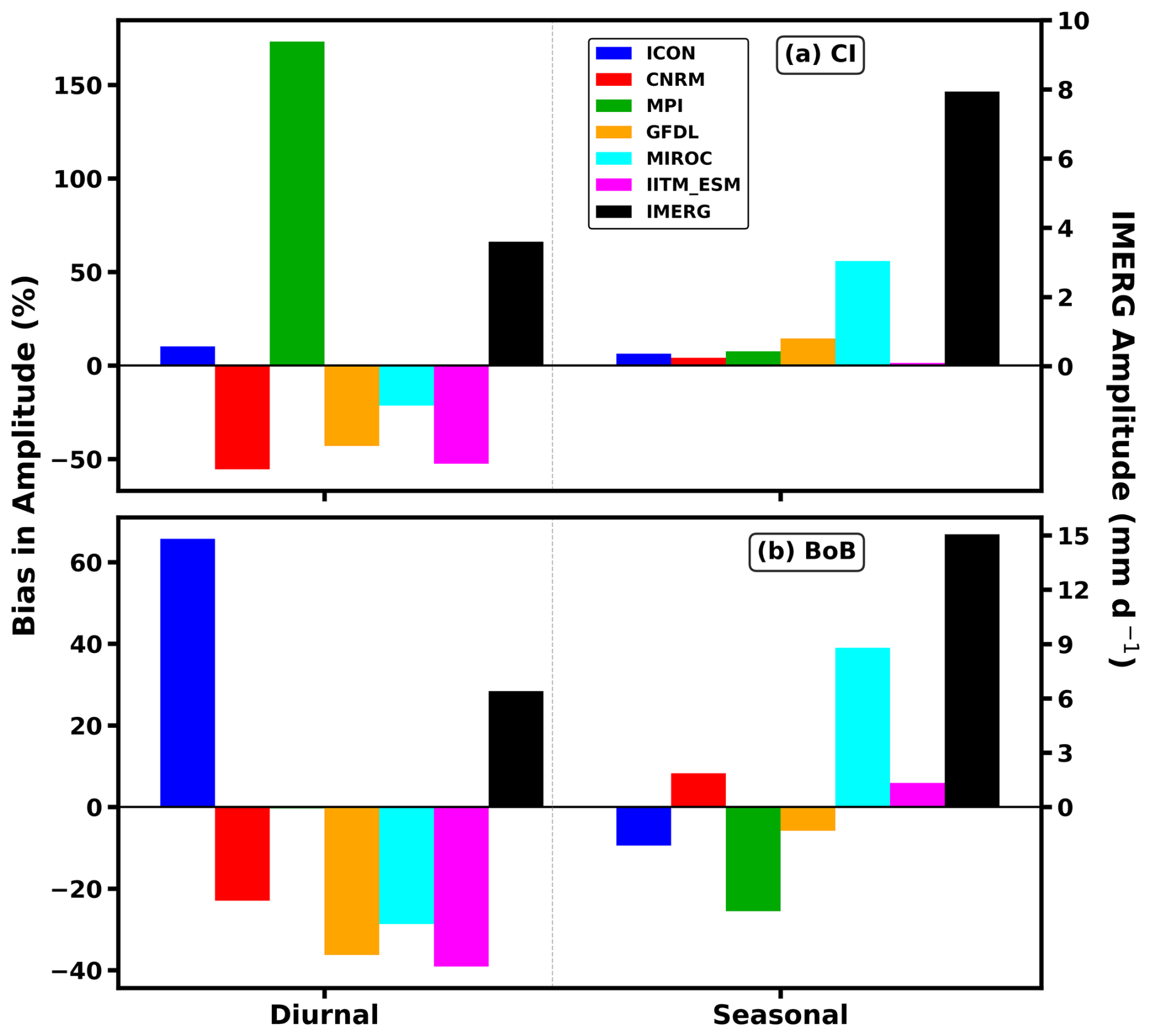
Figure 14 Same as Fig. 13, but for percentage climatological JJAS rainfall amplitude bias relative to IMERG at the diurnal and seasonal (JJAS) timescales, which are phase-locked to the diurnal and annual cycles, respectively.

Over land, ICON exhibits modest amplitude biases at both diurnal and seasonal scales (within ∼ 5 %–10 %), consistent with its relatively balanced multiscale variance structure. In contrast, MPI shows a pronounced overestimation of diurnal amplitude (> 150 %), directly mirroring its excessive diurnal variance and reflecting overly sensitive convective triggering within a mass-flux framework. The remaining models (CNRM, GFDL, MIROC, and IITM-ESM) generally underestimate diurnal amplitude, with the largest reduction in CNRM (∼ 50 %, corresponding to ∼ 2 mm d⁻¹ relative to an observed ∼ 4 mm d⁻¹). Notably, these sub-daily amplitude errors substantially diminish at the seasonal scale, indicating that much of the diurnal bias averages out over the monsoon period. An exception is MIROC, which exhibits a stronger seasonal amplitude bias (∼ 50 %, ∼ 4 mm d⁻¹), consistent with its enhanced lower-frequency variance discussed earlier.

Over the ocean, ICON displays a strong positive diurnal amplitude bias (∼ 60 %) over the BoB, reinforcing the large diurnal variance excess identified in Fig. 13 and its earlier diagnosed diurnal rainfall enhancement. This behavior likely reflects limitations of the AMIP configuration, where prescribed SSTs may exaggerate atmospheric responsiveness in strongly coupled regions. As over land, ICON's amplitude bias reduces substantially at the seasonal scale. Most other CMIP6 models underestimate oceanic diurnal amplitude (10 %–40 %, with MIROC showing the largest reduction), and seasonal biases generally decrease relative to diurnal errors, though MIROC and MPI retain noticeable seasonal-scale deviations.

Taken together, the amplitude diagnostics confirm that errors at the phase-locked endpoints are associated with the distribution of variance across the intermediate synoptic and intraseasonal bands. Models with exaggerated diurnal amplitude often show distorted 2–7 d synoptic and 10–20 d high-frequency MISO variance, whereas amplified seasonal amplitude tends to accompany enhanced lower-frequency intraseasonal variability. Accurate representation of these temporal endpoints is therefore important for maintaining a physically consistent partitioning of monsoon rainfall variability across temporal scales.

It is worth noting that the substantially larger diurnal variance bias relative to the amplitude bias (e.g., ∼ 180 % versus ∼ 60 % over the BoB in ICON) reflects the quadratic relationship between amplitude and variance. Because variance scales with the square of amplitude, even moderate increases in diurnal intensity can produce disproportionately large increases in variability. This indicates that the model enhances day-to-day fluctuations of the diurnal cycle more strongly than the mean diurnal rainfall amount itself, implying an over-responsive high-frequency convective adjustment rather than a simple uniform increase in rainfall.

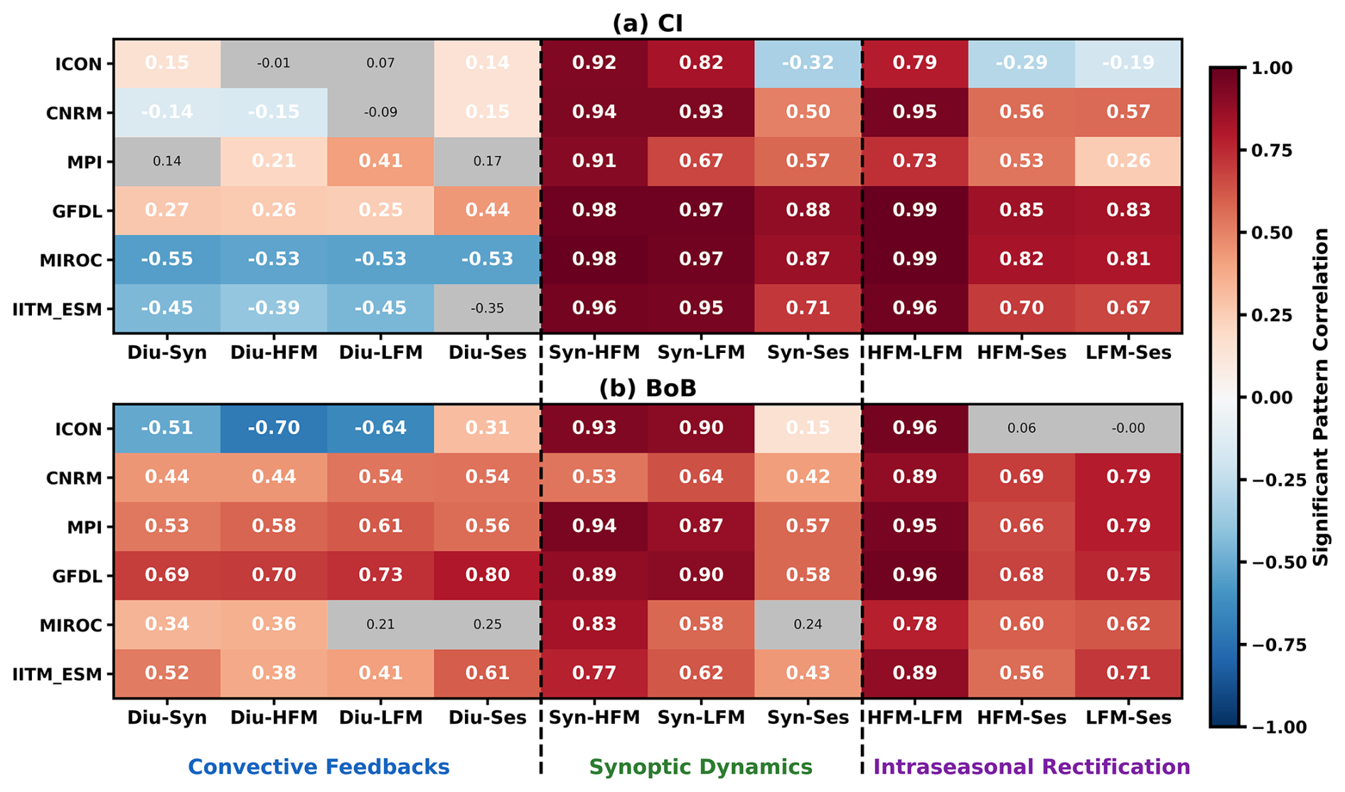
Figure 15 Heatmap of spatial pattern correlation coefficients among the relative bias fields of different scales. Correlations significant at the 95 % confidence level are highlighted in bold white font, while non-significant cells are masked in gray (small black font). For clarity, the heatmap is divided into three scale-dependent regimes: convective, synoptic, and intraseasonal. The abbreviations Diu, Sys, HFM, LFM, and Ses represent the diurnal, synoptic, high-frequency MISO (10–20 d), low-frequency MISO (20–100 d), and seasonal scales, respectively.

To examine whether scale-wise rainfall errors occur independently or as coherent multiscale structures, two complementary diagnostics are used. First, the percentage contribution of each timescale to the total variance bias is shown over CI and BoB to identify the dominant source of error within each model (Fig. S6). This diagnostic shows that the leading contribution differs by model and region, with errors dominated by different scales over CI and the BoB, while seasonal-scale errors generally contribute the least across most cases. Second, spatial pattern correlations among the relative variance-bias fields are shown in Fig. 15 to assess whether errors at different timescales are geographically co-located. The correlations are grouped into three regimes: convective feedbacks, synoptic dynamics, and intraseasonal rectification. In the convective-feedback regime, which links diurnal errors with lower-frequency biases, a clear land–ocean contrast emerges. Over CI, correlations are generally weak, negative, or only slightly positive, indicating that diurnal errors over land are not strongly co-located with synoptic, intraseasonal, or seasonal errors. This behaviour is seen in ICON, CNRM, MIROC, and IITM-ESM, while MPI and GFDL show relatively stronger positive associations. Over the BoB, most models, including CNRM, MPI, GFDL, MIROC, and IITM-ESM, show positive correlations, suggesting that oceanic diurnal errors are more closely aligned with lower-frequency rainfall errors. ICON is an exception, with negative diurnal–synoptic and diurnal–MISO correlations over the BoB, indicating that regions of enhanced diurnal variance tend to coincide with weaker lower-frequency variability.

In the synoptic-dynamics and intraseasonal-rectification regimes, correlations are mostly positive in the CMIP6 models, indicating that synoptic, MISO, and seasonal rainfall errors are generally co-located. This correspondence is particularly evident in GFDL, MIROC, MPI, and IITM-ESM, although the strength of the relationship varies by region and scale pair. ICON shows a different structure, with weak or negative correlations over CI and only weak to moderate positive correlations over the BoB. These relationships should be interpreted as diagnostic spatial associations rather than direct causal pathways. Nevertheless, they indicate that seasonal rainfall errors are not controlled by a single timescale; instead, each model exhibits a distinct partitioning of rainfall variability across diurnal, synoptic, and intraseasonal bands.

4 Summary and Conclusions

This study evaluates the capability of a medium-resolution (40 km), non-hydrostatic global model (ICON) to simulate ISMR arising from complex multiscale interactions spanning diurnal to seasonal timescales. ICON is examined as a test case for next-generation dynamical cores and is systematically compared with a suite of five CMIP6-class models (CNRM, MPI, GFDL, MIROC, and IITM-ESM) having horizontal resolutions from 50 to 190 km. All models are analyzed in AMIP configuration against high-resolution IMERG observations (∼ 10 km) over a common 17-year period (1998–2014), allowing isolation of atmospheric sources of rainfall bias under prescribed SST forcing. The results reveal that monsoon rainfall errors are inherently multiscale and strongly shaped by land–ocean contrasts, indicating that biases emerge differently across convective, synoptic and seasonal regimes. At the diurnal scale, model behavior diverges sharply depending on convective formulation and surface coupling. ICON shows the most realistic continental diurnal cycle, with modest amplitude biases (∼ 5 %–10 %) and limited phase errors that allow coherent afternoon–evening convection over land. However, over the BoB it substantially overestimates diurnal amplitude (∼ 60 %) and variance (∼ 180 %). In the present 40 km configuration, these biases are likely linked to the convective parameterization (Tiedtke–Bechtold mass-flux scheme). Previous studies have shown that convective parameterizations in medium- to coarse-resolution climate models tend to produce overly frequent precipitation and exhibit strong sensitivity to low-level moisture convergence, leading to excessive rainfall and an amplified diurnal cycle (e.g. Tao et al., 2023; Christopoulos and Schneider, 2021). While studies based on convection-permitting (∼ 2.5 km) ICON configurations attribute similar oceanic wet biases to overactive warm-cloud microphysics and excessive rainfall from shallow and congestus clouds (Prein et al., 2026), such mechanisms might not directly applicable here due to the reliance on parameterized convection at coarser resolution.

MPI exhibits the strongest land diurnal bias, with amplitude overestimation exceeding 150 % and an early rainfall phase. These errors arise because convection remains unresolved even at higher resolution, leaving rainfall characteristics largely controlled by resolution-insensitive parameterizations (Hertwig et al., 2015). Previous studies have also reported excessive convective rainfall over the Indian region in earlier versions of MPI (Chaudhari et al., 2019), consistent with the large diurnal-amplitude overestimation seen here. This suggests that higher horizontal resolution alone is insufficient to remove rainfall biases when deep convection remains parameterized. Resolution increases can redistribute rainfall between convective and large-scale components without necessarily improving precipitation timing or intensity, because convective triggering, CAPE buildup, and cloud–microphysical processes remain important controls (Bechtold et al., 2004; Rio et al., 2009; Stevens et al., 2013; Hertwig et al., 2015). Separating the relative roles of large-scale circulation, convective parameterization, and microphysics would require targeted sensitivity experiments and is beyond the scope of the present study. Over ocean, MPI underestimates diurnal variability, indicating weak nocturnal convective organization. CNRM shows premature daytime triggering over land and failure to initiate nocturnal convection above the boundary layer, resulting in weakened evening rainfall (Watters et al., 2021) and over ocean, its relatively smaller phase errors suggest somewhat improved nocturnal organization, though amplitude biases persist. The similar early land convection in GFDL is consistent with the behaviour expected from quasi-equilibrium convective closure, which can trigger rainfall before sufficient boundary-layer moistening and instability have developed. Its nocturnal rainfall deficit further suggests limitations in representing cold-pool dynamics and mesoscale lifting processes that help sustain nighttime convection (Zhang et al., 2024). Over the ocean, additional biases may arise from boundary-layer and cloud-microphysical processes that affect radiative balance and marine convection (Donner et al., 2011).

In MIROC6, biases in precipitation timing and intensity primarily arise from convection parameterizations. Despite the introduction of shallow convection schemes to enhance moisture mixing and reduce low-level cloud biases, these remain key tuning factors for rainfall distribution. Persistent deficiencies in vertical moisture mixing and convective triggering lead to timing errors, including an unrealistically early precipitation peak (Tatebe et al., 2019). IITM-ESM biases stem from its relatively coarse horizontal resolution (∼ 2°) and limitations in cloud and convection parameterizations. Despite improvements from the revised Simplified Arakawa–Schubert (RSAS) scheme, deficiencies in cloud microphysics contribute to a persistent dry bias. Previous studies have also documented a tendency of SAS and RSAS based schemes to produce dry biases over the Indian land region (e.g. Pokhrel et al., 2016; Swapna et al., 2018). In addition, inaccuracies in humidity fields and large-scale tropical circulation weaken moisture transport and convergence, compounded by the poor representation of key regional circulation features essential for realistic monsoon rainfall (Prajeesh et al., 2022). These deficiencies likely contribute to a weaker and less well-phased diurnal cycle in the model.

Together, these results indicate that diurnal rainfall biases are not determined by the parameterization framework alone, but also by its interaction with land–atmosphere processes. Over oceanic regions such as the Bay of Bengal, however, the role of air–sea coupling in modulating diurnal rainfall biases cannot be fully assessed within the prescribed-SST AMIP framework and requires coupled simulations.

At synoptic timescales (2–7 d), observed variance over land is dominated by monsoon low-pressure systems and mesoscale convective systems. ICON maintains realistic spatial organization, though with slightly reduced magnitude, suggesting moderate suppression of organized disturbances. MPI, in contrast, substantially suppresses synoptic variability, consistent with weak representation of organized disturbance growth. The remaining models either redistribute excessive power into intermediate (10–20 d) bands or fail to sustain coherent synoptic-scale evolution. Over the ocean, a similar tendency emerges, with several models underestimating synoptic variance, indicating weak organization of marine convective systems and limited maintenance of large-scale disturbances.

At intraseasonal scales (10–20 and 20–100 d), deficiencies become more systematic, with many CMIP6 models known to exhibit conspicuous phase shifts in low-frequency 30–60 d ISOs that lead to artificially extended early-season dry spells (Singh, 2023). Over land, variance redistribution differs across models but remains secondary to oceanic errors. Over the BoB and equatorial Indian Ocean, most models underestimate the 20–100 d band by ∼ 30 %–60 %, indicating weak low-frequency MISO variability in the prescribed-SST AMIP configurations. The absence of interactive air–sea coupling may contribute to this bias, but testing this hypothesis would require comparison with coupled simulations. Coarser-resolution models tend to amplify intermediate (10–20 d) bands, whereas higher-resolution configurations often underestimate low-frequency variability. These scale-dependent imbalances influence seasonal rainfall accumulation and migration.

Seasonal rainfall emerges as the cumulative imprint of these multiscale imbalances. Models maintaining proportionate energy partitioning across scales, most notably ICON shows strong spatial agreement with IMERG (PCC ≈ 0.85; RMSE ≈ 2.3 mm d⁻¹) and realistic annual migration, including September withdrawal. GFDL also performs reasonably well, though with a slightly broader seasonal extent. MPI underestimates synoptic variability and shows early withdrawal in the annual cycle. MIROC and IITM-ESM exhibit enhanced intermediate-frequency variance that contributes to seasonal amplitude distortions (approaching ∼ 40 %–50 % in some regions). CNRM maintains reasonable timing but overestimates rainfall over key oceanic regions. Amplitude diagnostics indicate that diurnal amplitude biases generally reduce at the seasonal scale, suggesting that sub-daily intensity errors partly average out over the monsoon season. However, models with enhanced intermediate-frequency variance retain noticeable seasonal amplitude deviations.

This study demonstrates that realistic simulation of monsoon variability across weather-to-seasonal timescales depends not only on seasonal-mean rainfall accuracy but also on maintaining physically consistent cross-scale organization. The results further indicate that higher horizontal resolution alone is insufficient to remove rainfall biases when deep convection remains parameterized. Recent ICON sensitivity experiments show that the impact of grid spacing on monsoon rainfall is region-dependent and non-systematic, with some aspects of the diurnal cycle improving while biases in mean precipitation and variability can be amplified (Pothapakula et al., 2026). Thus, differences among the models analysed here should be interpreted in terms of model configuration, including dynamical core, convective parameterization, microphysics, and circulation–rainfall coupling, rather than resolution alone. While non-hydrostatic dynamics at 40 km contribute to improved continental convection, ICON’s performance also reflects its well-tuned physical parameterizations, benefiting from its development within a numerical weather prediction framework, which enables a more realistic representation of mesoscale processes and their interactions with larger scale circulation. However, persistent oceanic biases highlight remaining challenges in convective organization, cloud microphysics, and air–sea coupling. Across the CMIP6 ensemble, biases in convective triggering, shallow-to-deep transition, mesoscale system organization, and boundary-layer–radiative coupling are likely to play an important role in shaping the fidelity of scale interactions. Future progress requires explicit diagnosing of cross-scale interactions rather than scale-isolated evaluation. Approaches such as Multivariate Empirical Mode Decomposition (MEMD) offer a promising framework to diagnose nonlinear variability redistribution among diurnal, synoptic, and intraseasonal modes. Such scale-aware diagnostics can help distinguish locally generated errors from those arising through multiscale interaction, providing targeted guidance for improving convective parameterizations, boundary-layer processes, microphysics, and coupled ocean–atmosphere representation. Advancing these diagnostics is essential for achieving physically consistent and societally relevant prediction of the Indian Summer Monsoon across weather-to-climate timescales.