Interhemispheric perspective on the most extreme surface winds in the storm tracks

Extratropical cyclones occur most frequently over the oceans, where they cause the strongest extreme surface winds. In this study, we investigate extreme surface winds during winter months in the Northern and Southern Hemispheres, when the wind storms are the strongest. The analysis focuses on storm tracks over the North Atlantic, North Pacific and Southern Ocean. We use ERA5 reanalysis data to make composites of extratropical cyclones that cause the top 100 most extreme surface wind events from 1979 until 2020 (“top 100 extremes”). We focus on large-scale atmospheric processes and find that the most prominent large-scale feature of the top 100 extremes in each basin is the presence of a pre-existing downstream cyclone a few days before the time of the maximum surface winds. Pre-existing cyclones are situated poleward and eastward of the top 100 extremes and their presence is consistent with strong upper-level winds and potential vorticity anomalies. Differences between the basins and hemispheres are quantitative. The top 100 extremes in the Northern Hemisphere develop in an environment with higher mid-tropospheric Eady growth rates, higher deepening rates and stronger surface wind speeds around the cyclones than in the Southern Hemisphere. Furthermore, we run the general circulation model ISCA with different boundary conditions to investigate their influence on the basin-wide extreme surface winds. We find a strong positive correlation between basin-wide extremes in mid-tropospheric Eady growth rates and surface winds. Zonalizing sea-surface temperatures across tropical and extratropical regions greatly reduces the differences in extreme surface winds between the North Atlantic and North Pacific; inter-hemispheric differences in extreme surface winds between the North Atlantic and Southern Ocean are greatly reduced when sea-surface temperatures are zonalized globally and made hemispherically symmetric, and orography is flat.

1 Introduction

Extratropical cyclones (hereafter, cyclones) are associated with a variety of extreme weather events, including extreme precipitation and windstorms (e.g. Catto et al., 2012; Pfahl and Wernli, 2012; Dowdy and Catto, 2017). Cyclones most frequently occur over the oceans, in regions known as storm tracks. Surface winds associated with oceanic cyclones are crucial for air-sea interactions, generating ocean waves which help determine surface roughness (Donelan et al., 1993), and controlling turbulent fluxes of energy (Hsiung, 1986) and CO₂ (Wanninkhof and McGillis, 1999) between the atmosphere and the ocean. Oceanic surface winds are also important to marine ecosystems (Lacour et al., 2017) and to economic activities such as wind power generation (Liu et al., 2008) and shipping (Cardone et al., 2015). Moreover, cyclones that develop over the oceanic storm tracks and make landfall pose a major socioeconomic hazard (e.g. Ulbrich et al., 2013a; Shimkus et al., 2017).

Here, our focus is on understanding the large-scale dynamical processes leading to extreme surface winds in midlatitudes. This improved understanding may ultimately help alleviate the biases and uncertainty that affect projections of extreme surface wind changes in future climates (Catto et al., 2019; Seneviratne et al., 2021). We are particularly interested in the relationship between extreme winds and the cyclones that drive them. We focus on the main ocean basins, where cyclones are most plentiful and free from the complexities of interaction with continental topography and surface roughness, making results more statistically significant and simpler to interpret physically.

We take a comparative approach, aiming to gain new insight by investigating similarities and differences between the major storm track regions. While the American and Eurasian landmasses confine the Northern Hemisphere (NH) storm tracks to form distinct North Atlantic (NA) and the North Pacific (NP) storm tracks, the limited land area of the Southern Hemisphere (SH), on the other hand, yields a single Southern Ocean (SO) storm track with weak zonal structure. Cyclones in all these ocean basins arise due to the same basic baroclinic instability process, but differences in surface boundary and upstream conditions in the different storm tracks influence their local statistics.

In particular, bulk metrics such as zonally-averaged, vertically-integrated eddy kinetic energy or median annual surface winds are larger in the SO than in the NH basins, which is why the SO is often considered the stormier hemisphere (Shaw et al., 2022; Chemke et al., 2022). However, extreme surface winds are stronger over the NH storm tracks (Stanković and Caballero, 2025), particularly the NA. This is true across reanalysis and observational products, and mainly stems from stronger extreme winds in the vicinity of winter cyclones in the NH. Hence, at least when measured by their surface wind speeds, extreme cyclone intensities are greater in the NH than in the SH.

Our aim in this study is to better understand the reasons for these opposite inter-hemispheric asymmetries in mean and extreme oceanic winds. We address the following specific questions:

1. What are the large-scale processes leading to the generation of cyclones causing extreme surface winds in each storm track?

2. What differences in these large-scale processes can help explain the greater frequency of extreme surface winds in the Northern than in the Southern Hemisphere?

3. How are these dynamical differences related to differences in surface boundary conditions across the storm track basins?

We address these questions by focusing on winter seasons, when cyclones are the strongest in both hemispheres, and we select the 100 historical cyclones associated with the strongest extreme surface winds in each storm track region (hereafter top 100 extremes). We analyze large-scale fields through time-lagged composite analysis.

We address the last question by using an intermediate-complexity climate model. Use of climate models with varying complexities has long been recognized as a way to deepen the understanding of the climate system (a good overview is provided in Vallis, 2016). Furthermore, climate modeling is also widely applied to study the storm tracks (Shaw et al., 2016). Boundary conditions, such as orography, sea surface temperatures, land-sea contrast and ice cover have been varied to investigate their effects on both the individual and hemispheric storm tracks (e.g. Brayshaw et al., 2009, 2011; Patterson et al., 2020; White et al., 2021; Shaw et al., 2022; Hay et al., 2025). Following these examples, we use a climate model to test whether the boundary conditions documented to be of a general importance for the storm track dynamics also influence the hemispheric differences in extreme surface winds.

The paper is structured as follows. The data and methods we use are described in Sect. 2, after which we present our main results in Sect. 3. We summarize the results, discuss their implications and provide a future outlook in Sect. 4. Finally, we list our main findings in Sect. 5.

2 Data and Methods

2.1 ERA5

We employ the ERA5 global atmospheric reanalysis from the European Centre for Medium Range Weather Forecasts (Hersbach et al., 2020) spanning 1979–2020 to study the most extreme historical cyclones. Even though the ERA5 reanalysis covers the period from 1940 to present day, we focus on the period after 1979 because it assimilates satellite observations which are crucial for robustly representing sparsely observed regions in the SH. On the other hand, we focus our analysis to the period up until 2020 because the output provided by the cyclone-tracking algorithm (described below) ends with 2020. The reanalysis has hourly temporal and 0.25° (∼31 km) spatial resolution. We focus on the analysis of winter seasons, defined as December–February in the NH and June–August in the SH. We use surface windspeed calculated as $(u_{\mathrm{10}}^{\mathrm{2}}+v_{\mathrm{10}}^{\mathrm{2}}{)}^{\mathrm{1}/\mathrm{2}}$, where u₁₀ and v₁₀ are 10-m zonal and meridional wind components taken from ERA5. We additionally consider 250 hPa wind speed, potential vorticity (PV) from 300 to 200 hPa (4 vertical levels) and mean sea level pressure (MSLP). We further calculate the instantaneous, dry Eady growth rate as: $\text{EGR}=\mathrm{0.31}\frac{f}{N}\frac{\partial \left|\mathit{u}\right|}{\partial z}$ between 500–850 hPa, calculated as in Besson et al. (2021); Stanković and Caballero (2025). Here f denotes Coriolis parameter, $\left|\mathit{u}\right|$ the magnitude of horizontal wind speed, z is the vertical coordinate and $N=\sqrt{\frac{g}{\mathit{\theta }}\frac{\partial \mathit{\theta }}{\partial z}}$ the Brunt-Väisälä frequency, commonly used as a measure of static stability, with g being gravitational acceleration and θ potential temperature. We use the instantaneous EGR to avoid biases connected to nonlinearities and covariances observed with time-mean EGR (Simmonds and Lim, 2009). Finally, our analysis includes vertically integrated eddy kinetic energy, $\text{EKE}={\int }_{p_{\mathrm{1}}}^{p_{\mathrm{2}}}\frac{u^{\prime \mathrm{2}}+v^{\prime \mathrm{2}}}{\mathrm{2}g}\mathrm{d}p,$ where u^′ and v^′ are zonal and meridional deviations from local monthly means for each given month at each grid cell, p₁=1000 hPa and p₂=200 hPa. The way we calculate u^′ and v^′ is common in studies like ours (e.g. Park and Kim, 2021; Shaw et al., 2022) and while it can cause some discontinuities for the events that occur at month boundaries, we do not expect these discontinuities to qualitatively alter our results.

2.2 Selection and tracking of top 100 extremes in each basin in ERA5

We identify storm tracks as areas where the annual 98th percentile of daily maximum surface windspeed exceeds 18 m s⁻¹ in ERA5. This is the same criterion used in Stanković and Caballero (2025) and it identifies three separate storm track regions with comparable statistics, one each in the North Atlantic, North Pacific and Southern Ocean (see Fig. 1a). We use this criterion based on surface winds because our main scientific question is the understanding of surface wind extremes, but the storm tracks we identify coincide with storm tracks identified by using other measures (Hoskins and Hodges, 2002, 2005; Shaw et al., 2016). As our focus is on the large-scale dynamics, we repeat the procedure of Stanković and Caballero (2025) and exclude regions that are within 300 km distance from the coasts of Greenland and Antarctica which feature very strong surface winds primarily caused by mesoscale processes.

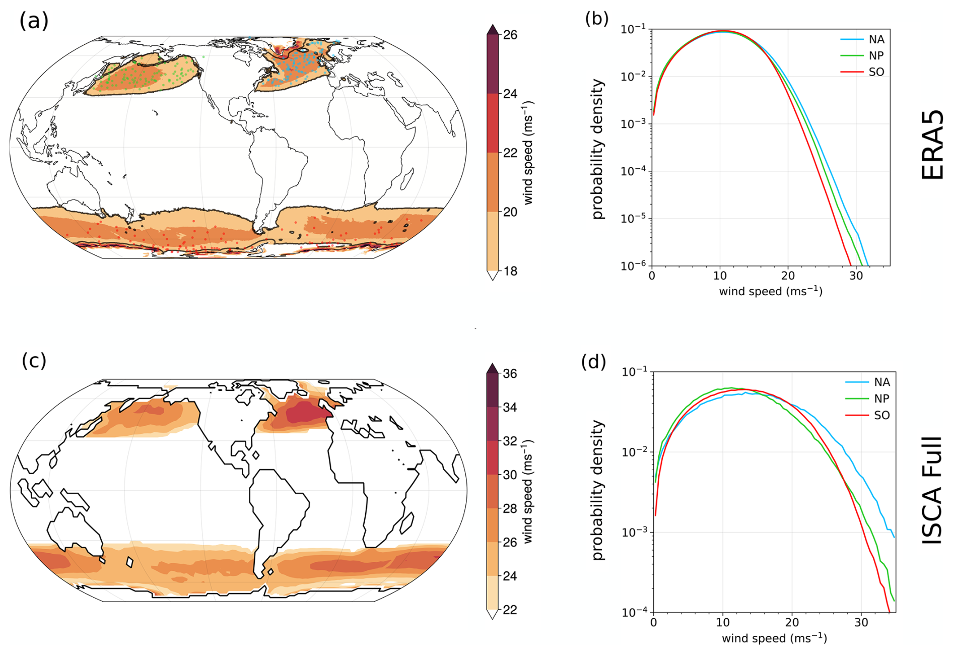
Figure 1 Maps of annual 98th percentile (a, c) and probability density functions (b, d) of daily-maximum and 6-hourly (a, b) 10-m windspeed in ERA5 and (c, d) windspeed at the level closest to the surface in ISCA Full experiment, respectively. Probability density functions are made from windspeed sampled in the regions marked in (a) and (c) in the North Atlantic (NA, blue), North Pacific (NP, green) and Southern Ocean (SO, red). Black contours in (a) show the selected storm track regions used for calculating severity in ERA5, while the selected storm track regions in ISCA correspond to the colored areas in (a). Green, blue and red dots over the storm track regions in (a) show the locations of cyclone centers of the top 100 extremes at the time of maximum severity.

We identify cyclones in ERA5 using cyclone tracks produced by Beran et al. (2024). This feature-tracking algorithm applies topological methods (Engelke et al., 2021; Nilsson et al., 2022) to track MSLP minima in ERA5 and provides hourly global output. It improves the method of Hanley and Caballero (2012a) and it is primarily developed to better represent multi-centre cyclones, which are comprised of several MSLP minima. Therefore, in the event of two cyclones merging, the information about the centres of the merged cyclones is retained and they are collectively seen as a part of the same, multi-centre cyclone structure. The same algorithm was previously used in Stanković and Caballero (2025). The choice of the tracking algorithm could potentially have an influence on the results. However, tracking intercomparison studies consistently show a strong agreement between different tracking algorithms in representing deep, well developed cyclones (Neu et al., 2013; Ulbrich et al., 2013b; Messmer and Simmonds, 2021). Therefore, as our focus lies on some of the most extreme cyclones in each basin, we argue that results should not be overly sensitive to the choice of tracking algorithm.

We find the cyclones associated with the top 100 most extreme wind events in each basin (i.e. top 100 extremes) in two steps. In the first step, we investigate all winter days within the previously defined storm track basins and find the top 100 most extreme wind events. In the second step, we connect these wind events to the cyclones which we further analyze.

The top 100 most extreme wind events are calculated by ranking every winter day in each storm track basin with respect to a wind severity quantified by a meteorological wind severity index. This procedure also consists of two steps. We first calculate a daily meteorological wind severity index for each grid cell within the storm track regions. As the wind severity index is only calculated if the daily maximum windspeed exceeds the local 98th percentile (see the Eq. 1 below), the index is equal to zero over a majority of the grid cells on any given day. An extreme wind footprint is defined as a contiguous region of wind exceedances over the local 98th percentiles, namely an area consisting of connected non-zero grid cells (no minimum area threshold is imposed on the footprint size). Our last step for finding the top 100 most extreme wind events consists of calculating the wind severity index for each wind footprint. As two or more extreme wind-causing cyclones can be simultaneously present in the same basin on a given day, there can be more than one extreme wind footprint. In this case, we only select the footprint with the maximum value of severity for that day (a visual illustration of the method can be found in Fig. 2 of Stanković et al., 2024). Lastly, we choose the 100 d with the highest severities in each basin.

We calculate a meteorological wind severity index (S) as follows:

$$\begin{array}{}\text{(1)}& {\displaystyle }{\displaystyle }\mathrm{S}=\sum _{i\in \text{footprint}}{\left({\displaystyle \frac{v_i}{v_{{\mathrm{98}}_i}}}-\mathrm{1}\right)}^{\mathrm{3}},\end{array}$$

where i indexes all the grid cells within the wind footprint, v_i is daily maximum 10-m wind speed at grid point i, $v_{{\mathrm{98}}_i}$ is the local 98th percentile with respect to the winter climatology from 1979 to 2020. This index, or similar forms of it, have long been used to study windstorms associated with cyclones (e.g. Klawa and Ulbrich, 2003; Leckebusch et al., 2008; Hanley and Caballero, 2012b; Moemken et al., 2024; Flynn et al., 2025). Although the wide-spread use of this index stems from its usefulness in modeling insurance-related windstorm losses, it also has physical grounding as the cube of the wind speed represents the flux of kinetic energy. Furthermore, it is reliant on an extreme percentile threshold which motivates its use for extreme weather analysis. Therefore, we use it to rank extreme wind events even though we are not directly interested in analyzing insurance losses. This same procedure was adopted in Stanković et al. (2024) to identify extreme windstorms over the central North Atlantic.

After finding the top 100 most extreme wind footprints, we connect them to objectively identified cyclones. We examine the wind footprints during each of the top 100 d and find the time and location of the highest daily surface windspeed within them. Then, based on the objectively identified cyclone tracks, we identify the cyclone centre closest to the location of maximum windspeed and use it to follow the cyclone back in time.

2.3 Composite analysis

We compute cyclone-centered composites to identify the main large-scale flow features associated with the top 100 extremes in each basin. The convergence of latitude lines towards the poles necessitates regridding of meteorological fields to radial grids centered on the cyclone centers. To do this, we follow the grid transformation explained in detail in Appendix A of Bengtsson et al. (2007), often applied in studies like ours (e.g. Catto et al., 2010; Dacre et al., 2012; Laurila et al., 2021). Our composite analysis includes both the absolute values of the analyzed fields and their anomalies from the 1979–2020 climatology. We calculate climatologies by computing a 31-d running-mean of the daily means for calendar days of a given variable at every grid point and pressure level of interest. To test whether the anomalies from climatology are statistically significant, we construct for each basin and time step of interest, 100 randomly generated composites, each containing the same number of fields as the original composite. These composites are made by retaining the original cyclone centers but assigning each to a randomly selected winter date. Thus, at t=0 d, the 100 composites collectively sample 10 000 randomly selected dates. Anomalies are deemed statistically significant at the 1 % level after being corrected for false discovery (Wilks, 2016).

2.4 ISCA model and experiment setups

We perform sensitivity experiments using ISCA, an open-source modeling framework developed by Vallis et al. (2018). Our starting point is ISCA's default setup with realistic continents and prescribed sea-surface temperatures (SSTs) and ice fraction (Vallis et al., 2018). Prescribed SSTs and ice fraction used to force the model repeat annually, but vary monthly according to the monthly means of the years used in AMIP (Taylor et al., 2000). The model uses a spectral dynamical core to integrate the primitive equations. We analyze 6-hourly output of the model which we run at T42 horizontal resolution with an atmospheric model timestep of 720 s (12 min). The model parametrizes large-scale condensation and evaporation as in Frierson et al. (2006) and Vallis et al. (2018), radiation as in Clough et al. (2005) and also contains a simple representation of land and sea ice. It does not contain a representation of clouds, and instead assumes immediate precipitation with no explicit condensed water content in the atmosphere (Vallis et al., 2018). ISCA has been widely used to study different climates and is, in general, able to realistically represent Earth's climate (e.g. Vallis et al., 2018; Thomson and Vallis, 2018a, b; Patterson et al., 2020; White et al., 2024). More information about the model configuration is found in Vallis et al. (2018).

We first show that ISCA can be used to study wind extremes, as it represents well the annual and winter climatology of near-surface winds (see Fig. 1 and Sect. 3.2). We then vary boundary conditions to explore the effects they have on surface wind extremes over the storm track regions – a commonly used approach for studying storm track dynamics (e.g. Brayshaw et al., 2009, 2011; Shaw et al., 2016). As discussed in the Sect. 1, the previous literature suggests that the storm tracks are heavily influenced by different distributions of sea surface temperatures and the presence of orography and land surfaces. This motivates our ISCA experiments through which we test how different configurations of these boundary conditions influence climatologies of near-surface winds in different basins. Additionally, we design two experiments to test whether the differences in storm tracks are influenced by the presence of Greenland and its orography, which have previously been shown to influence large-scale circulation in the Northern Hemisphere (e.g. Jung and Rhines, 2007; White et al., 2019).

We run 11 different experiments, which are listed and described in the Supplement. For the brevity, however, we focus our analysis on the three experiments which we find to be the most consequential. We also briefly discuss the most salient conclusions of the additional experiments in the Results section. The three experiments we focus on are:

• Full, which uses the realistic representation of orography and SSTs and is similar to the control set-up used by Patterson et al. (2020);

• ZonalSST, where SSTs are zonalized in both the tropics and extratropics by taking a longitudinal mean across all ocean grid cells over each latitude;

• HemSymFlat, where zonalized SSTs are also hemispherically symmetrized by prescribing SSTs of each latitude in the NH to a corresponding latitude in the SH while respecting seasonality (i.e. latitudes with the same absolute values have same SST values in the NH and in the SH during their respective winters) and orography is made flat.

All experiments are run for 15 years, with the first two years (four in cases where SSTs are hemispherically symmetrized) disregarded as a spin-up time. The prescribed SSTs are shown and discussed in the Results section. The boundary layer parametrization schemes in the ISCA model do not produce 10-m wind speed as the model output. We instead use the windspeed at the level closest to the surface (973.1 hPa corresponds to the lowest full model level, diagnosed from ISCA's native sigma-pressure vertical coordinate) and refer to winds at this level as surface winds when we discuss ISCA results. Storm track masks are constructed similarly to ERA5. However, we expect the near-surface winds in ISCA to be less affected by surface friction, as the effects of the friction are not fully resolved. We therefore use a higher threshold of annual 98th percentile of near-surface winds for ISCA (21 m s⁻¹). Additionally, we do not exclude grid cells that are less than 300 km away from Greenland and Antarctica as in ERA5, since the much coarser resolution of the ISCA model does not resolve mesoscale features of these regions. We calculate a separate storm track mask for each ISCA experiment, in order to account for small changes in storm track areas due to the different boundary conditions.

3 Results

3.1 Composite analysis of top 100 extremes in each basin in ERA5

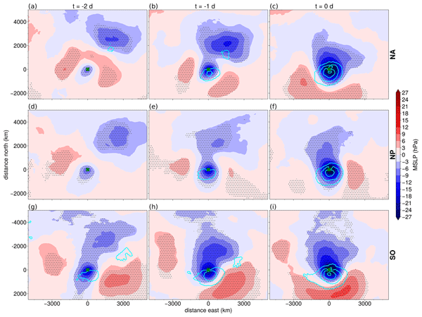
Figure 2 shows the development of the top 100 extremes in each basin as lagged composites of MSLP anomalies from climatology. The figure shows that in each basin and across hemispheres, the development of top 100 extreme cyclones occurs in the presence of a pre-existing cyclone located downstream of the developing extreme cyclone. This result generalizes our previous finding on the presence of pre-existing cyclones around top extremes in the NA (Stanković et al., 2024) to all major storm track basins. Close to the time of cyclogenesis ($t=-\mathrm{2}$ d, Fig. 2a, d, and g), these pre-existing downstream cyclones are poleward (note the reversal of the sign on y axis on Fig. 2g–i for the SO's composites) and eastward of the extreme cyclone (located at the centre of each panel). The extreme cyclones display initially weak and spatially limited anomalies at $t=-\mathrm{2}$ d, which then grow in size and intensity as they approach the pre-existing downstream cyclone. At t=0 d (Fig. 2c, f, and i), the two cyclones form a broad area of large negative MSLP anomalies. Around half of top 100 extremes in each basin form a multi-centre cyclone with pre-existing cyclones (49, 53, and 56 in the NA, NP, and SO, respectively, are classified as multi-centre cyclones by the cyclone tracking algorithm ±6 h around t=0 d). Thus, MSLP anomalies during the development of the top 100 extremes follow the same general pattern in all basins.

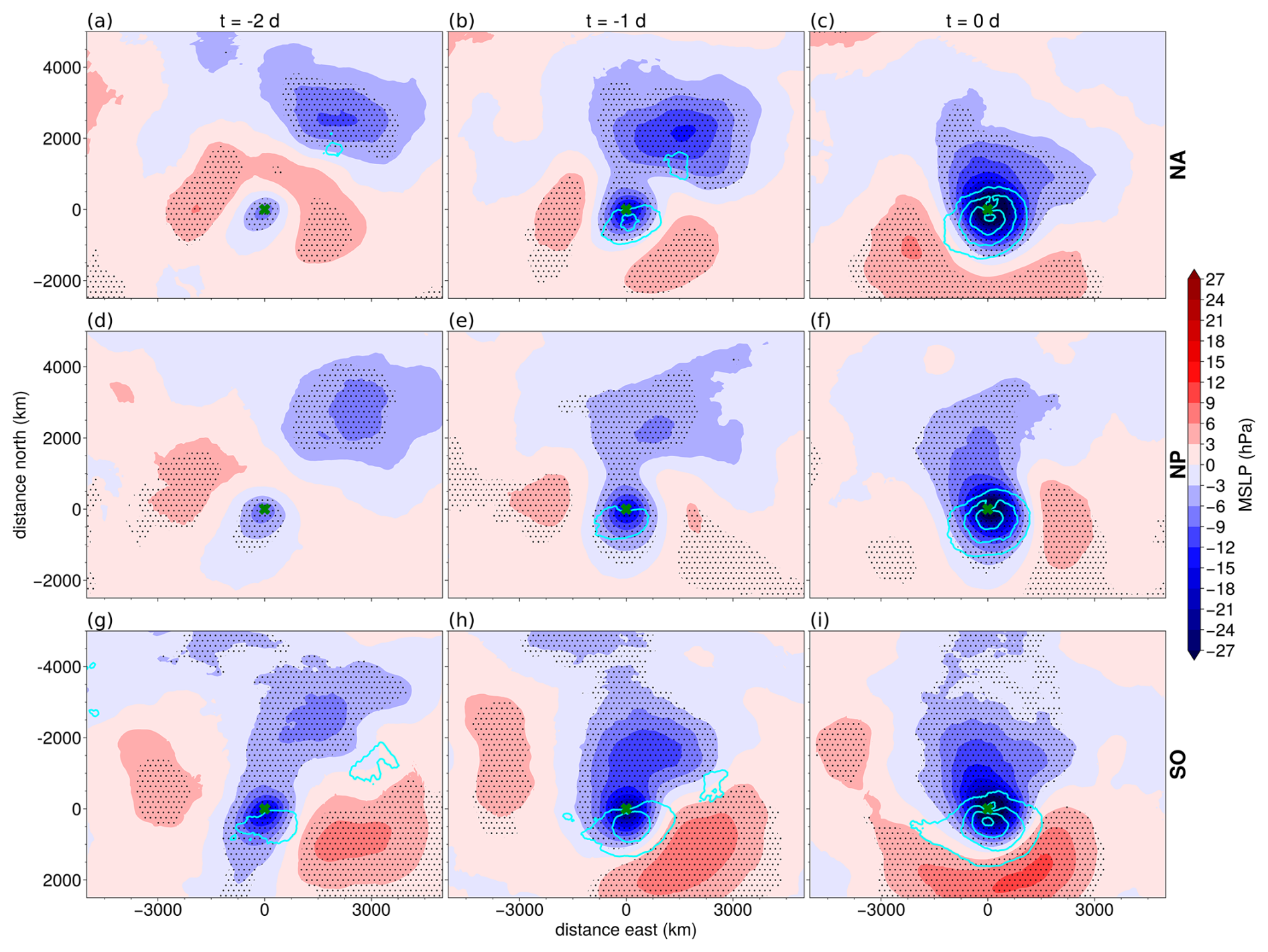
Figure 2 Composite MSLP anomalies in ERA5 relative to the 1979–2020 climatology for top 100 extremes in the NA (a–c), NP (d–f), and SO (g–i) centered on the cyclone locations from $t=-\mathrm{2}$ d to t=0 d. Lags are relative to the time of maximum 10-m wind speeds on the day with maximum severity. Green crosses denote locations of cyclone centers of top 100 extremes. Blue contours show the values of 10-m wind speeds, starting from 12 m s⁻¹ and increasing in steps of 3 m s⁻¹. Black dots show areas where MSLP anomalies are statistically significant at the 1 % level, corrected for false discovery (Wilks, 2016). The y axis for the SO composites (g–i) has been flipped so that the southernmost parts are at the top of the figures.

Figure 2 further shows that the intensification of 10-m wind speeds around top 100 extremes coincides with their deepening. A clearly defined area with 10-m winds exceeding 12 m s⁻¹ is detected equatorward of the cyclone centers at $t=-\mathrm{1}$ d in all basins (Fig. 2b, e, and h), and is already present in a more confined form in the SO at $t=-\mathrm{2}$ d (Fig. 2g). However, the largest intensification of 10-m wind speeds in all basins happens between $t=-\mathrm{1}$ d and t=0 d. At t=0 d (Fig. 2c, f, and i), a large footprint of strong 10-m wind speeds stretches from around 500 km poleward to 1500 km equatorward of the cyclone centres of top 100 extremes. At the same time, the highest values of 10-m wind speeds in all basins are close to and equatorward of the cyclone centres of top 100 extremes (Fig. 2c, f, and i).

Composites of upper-level fields, like their surface counterparts, also show qualitative similarity across basins (Figs. 3 and 4). The pre-existing downstream cyclone advects high-PV air equatorward generating a region of high PV gradients, consistent with positive upper-level PV anomalies around the location of the developing extreme cyclone in the days leading to peak surface winds (Fig. 3). However, quantitative differences between the hemispheres are more prominent than for MSLP (cf. Figs. 2 and 3). Upper-level PV poleward of the top 100 extremes is greater in the NH than in the SH, making the PV gradient in the NH much larger than in the SH. The strongest upper-level PV gradients are found in the NP. Quantitative differences are also observed in the upper-level PV anomalies around cyclone centers of the top 100 extremes, which have larger values in the NH at t=0 d (Fig. 3c, f, and i).

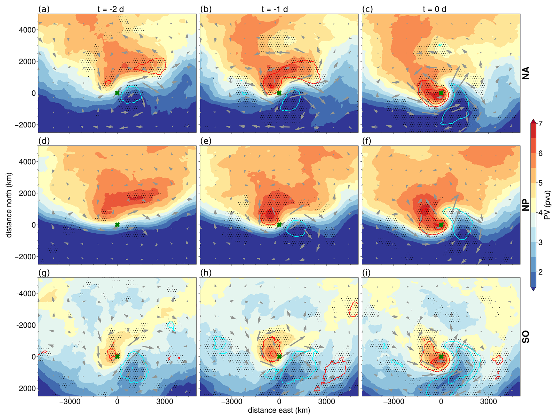
Figure 3 Upper-level composites for top 100 extremes in the NA (a–c), NP (d–f), and SO (g–i) centered on the cyclone locations from $t=-\mathrm{2}$ d to t=0 d. Colors show upper level PV (200–300 hPa mean) values, while red and blue contours show positive and negative upper level PV anomalies relative to the 1979–2020 climatology, respectively, every ±1 pvu and starting from ±1 pvu. Grey arrows show 250 hPa horizontal wind speed anomalies from climatology. Green crosses have the same meaning as in Fig. 2. Black dots show areas where upper level PV anomalies are statistically significant at the 1 % level, corrected for false discovery (Wilks, 2016).

Figure 4 shows further quantitative differences between the basins. Differences in the upper-level PV gradients shown in Fig. 3 translate into different intensities of the upper-level jet streaks (Fig. 4). Jet streaks are stronger in the NH than in the SH from $t=-\mathrm{2}$ d to t=0 d, and the strongest jet streak composites are in the NP. Consistent with higher expected values of wind shear below stronger jet streaks, composites of mid-tropospheric EGR show broader areas of large values in the NH (Fig. 4). Therefore, quantitative differences above the boundary layer are not only confined to around the tropopause, and are instead present throughout the free troposphere.

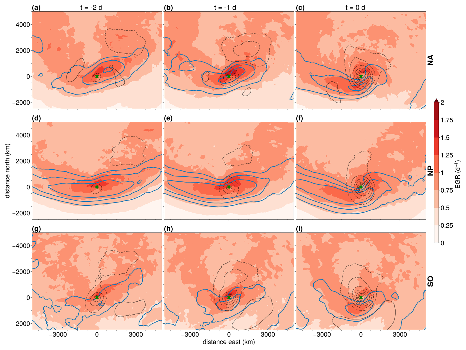
Figure 4 Composites of mid-tropospheric EGRs for top 100 extremes in the NA (a–c), NP (d–f), and SO (g–i) centered on the cyclone locations from $t=-\mathrm{2}$ d to t=0 d. Green crosses have the same meaning as in Figs. 2 and 3. Dark blue contours show the values of 250 hPa wind speeds, starting from 35 m s⁻¹ and increasing in steps of 10 m s⁻¹. Black contours show MSLP anomalies relative to the 1979–2020 climatology, every ±5 hPa and starting from ±5 hPa (dashed for negative anomalies).

In summary, while the extreme cyclones in our sample follow a qualitatively similar large-scale development in all basins, those in the NH are accompanied by larger upper-level PV gradients, stronger jet streaks and larger areas with high values of EGR. Can these differences account for the climatological hemispheric asymmetry in extreme surface winds, characterized by stronger surface winds around NH cyclones (Stanković and Caballero, 2025)? We investigate this by exploring the time-evolution of medians of EGR, EKE and 10-m winds in the 1,000-km footprint around cyclone centers of the top 100 extremes.

As shown in Fig. 5, median values of these fields around the centers of top 100 extreme cyclones indicate that these are more intense in the NH than in the SH, whether measured by column-integrated EKE or 10-m winds. Furthermore, mid-tropospheric EGR in the NH is consistently higher than in the SH in the days leading to peak severity (Fig. 5a). As the EGR is a proxy for the rate with which instabilities grow in a baroclinic atmosphere, higher EGR around a cyclone could, to first order, be understood as a greater potential for rapid intensification. This is supported by the time-evolution of cyclone intensity: the rate with which EKE rises between $t=-\mathrm{2}$ d and t=0 d is much greater in the NH (Fig. 5b). Consistently, there are almost twice as many explosively deepening cyclones among top 100 extremes in the NH than in the SO: 69 % and 75 % in the NA and the NP respectively compared to 38 % in the SO, with explosively deepening cyclones defined as those experiencing a decrease of the normalized values of 24-hourly MSLP greater than 24 hPa (Sanders and Gyakum, 1980).

It appears therefore that the main difference between the top 100 extremes in different basins is a quantitative one, characterized primarily by the mid-tropospheric baroclinicity measured by EGR. The presence of a pre-existing downstream cyclone that acts as to intensify the upper-level PV gradient and the jet steak, as seen in the composite analysis, can consequently also intensify the EGR. However, the absolute values of upper-level PV poleward of pre-existing cyclones are larger in the NH than in the SH (Fig. 3). This is another quantitative difference between the hemispheres which could potentially limit the effectiveness of pre-existing cyclones in increasing the upper-level PV gradients in the SO. This is important as the composites of EGR show that EGR has its highest values around the jet cores (Fig. 4) and stronger jet cores observed in the NH are associated with stronger vertical wind shear. As the vertical wind shear is the main component driving the differences in EGR between the hemispheres (the stability term plays a smaller role, see Supplement), the fact that the number of the top 100 extremes that deepen explosively is almost two times larger in the NH than in the SH can primarily be connected to the differences in the jet steak influenced by the presence of pre-existing downstream cyclones.

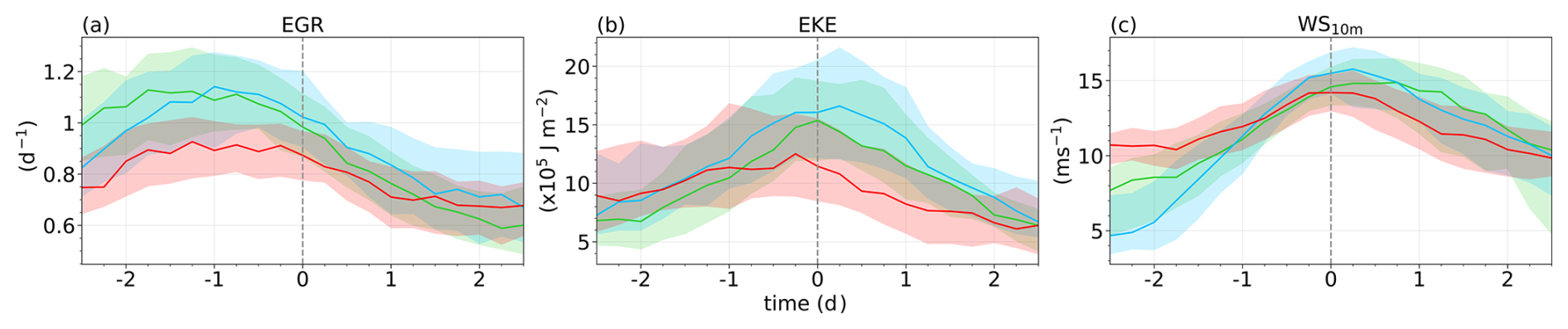
Figure 5 Time-evolution of median values in the 1000-km footprint around top 100 extremes of mid-troposhperic Eady growth rate (a), vertically integrated eddy kinetic energy (b), and 10-m wind speed (c). Colors signify the same basins as in Fig. 1a, while shading in (a–c) shows the area between 25th and 75th percentiles.

From a climatological perspective, winter basin-wide 98th percentiles of EGR correlate well with winter basin-wide 98th percentiles of 10-m winds, having the highest values in the NA, followed by the NP and then the SO (Supplement). Furthermore, to test whether the relationship between EGR and 10-m winds holds more generally, we identify a new group of cyclones in each basin. We find the new group of cyclones by identifying cyclone tracks for which the maximum value of median EGR around the cyclone centers during the cyclones' lifetimes is ≈30 % lower than in the case of top 100 extremes (Fig. 5a). Time-series of 10-m winds around the new group of cyclones confirm our expectation that the cyclones with lower maximum values of EGR also have lower 10-m winds during their lifetime (see Supplement). All of this motivates the usefulness of EGR as a predictor of extreme near surface winds and its use as a diagnostic to interpret differences between the basins in the ISCA experiments in Sect. 3.2.

3.2 ISCA experiments

First, we asses whether ISCA is a useful model to study surface wind extremes in the main storm track regions. We compute the winter PDFs of surface winds in the Full experiment and compare the results to ERA5. Figure 1d shows empirical PDFs of surface winds in the Full experiment. Not only is ISCA able to represent hemispheric asymmetry in extreme winds (i.e. stronger wind extremes in the NH, Fig. 1b), but it also correctly “ranks” the basins according to the strength of their wind extremes: In ISCA, the strongest wind extremes are in the NA, followed by the NP and the SO, as is consistently shown in reanalyses and observational products (Stanković and Caballero, 2025).

Second, we analyze the annual spatial distribution of 98th percentiles of surface winds in ISCA (Fig. 1c) and compare them to 98th percentiles in ERA5 (Fig. 1a). ISCA is able to realistically represent the spatial pattern of extreme winds. For instance, the highest values of the 98th percentiles in the NA are observed in the central NA region in both ERA5 and ISCA. At the same time, there are some spatial discrepancies between representations of storm tracks in ISCA and ERA5. Most notably, when compared to ERA5, the peaks of the 98th percentiles in ISCA are shifted equatorward in the Pacific sector of the SO and eastward in the NA and NP basins. In addition, while ISCA does reproduce the tilt of the NA storm track, the tilt is not as large as in ERA5. Many of the biases that ISCA has are not surprising as they are reminiscent of biases of other, more complex climate models (e.g. Shaw et al., 2016; Koskentausta et al., 2025). Since our goal is to better understand general differences between storm tracks in an idealized setting, we deem ISCA to be a suitable tool for this purpose.

Having built confidence that ISCA reproduces the main characteristics of surface winds in the storm track regions across the basins, we use ISCA to further study differences between the basins. In view of the ERA5 results, the main questions we aim to answer with ISCA experiments are: why are the surface wind extremes in the storm track regions stronger in the NH than in the SH; and why are they the strongest in the NA (and not in the NP)? In particular, how do differences between the boundary conditions which characterize the storm tracks (like the presence of orography or the spatial distribution of SSTs) affect the climatological distributions of the surface wind extremes within each storm track? To address this question, we run ISCA experiments where we change the boundary conditions and test their influence on the surface wind extremes. To quantify the influence of different experiment configurations on the surface wind extremes in the storm tracks, we measure both the absolute values of the winter basin-wide 98th percentiles of near-surface winds and how much the asymmetry between the basins (difference of the basin-wide 98th percentiles of near-surface winds in the NA and SO/NP divided by SO/NP) changes percentage-wise.

Figure 6a shows the absolute values of winter basin-wide 98th percentiles of surface winds for each selected experiment and percentage-wise difference in these values between the NA and the SO (Fig. 6a and b) and the NA and the NP (Fig. 6a and c). The asymmetry between the 98th percentiles in the NA and the SO is almost completely eliminated (reduced by 83 %) in the HemSymFlat experiment compared with the control experiment. The reduction in the asymmetry results from a combination of the 98th percentile decreasing in the NA and increasing in the SO. Half of the asymmetry reduction (41 %) is achieved by only zonalizing SST (ZonalSST experiment) although, in this case, mainly because of a decrease in the NA. Overall, the basin-wide 98th percentile of SO surface winds gradually increases for each new experiment set-up, but the largest increase occurs with HemSymFlat experiment.

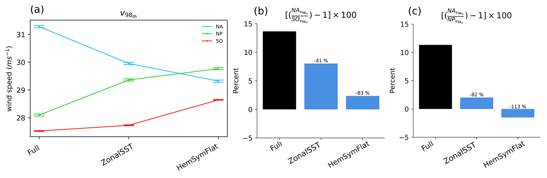
Figure 6 Absolute values of basin-wide 98th percentiles of surface wind speeds (a) and the relative difference in the percentile values between the North Atlantic and the Southern Ocean (b) and the North Atlantic and the North Pacific (c) with the selected ISCA experiments. Colors in (a) signify the same basins as in Figs. 1c and 5, while the horizontal lines above each value show the confidence interval at 1 % significance level computed with resampling 10 000 times. Percentage values above certain bars in (b) and (c) show a percentage difference in asymmetries compared to the Full ISCA experiment.

Differences in extreme winds between the two NH basins (NA and the NP) are almost completely removed (reduced by 82 %) in the ZonalSST experiment. This happens because the basin-wide 98th percentile of surface winds increases in the NP, while it decreases in the NA. Flattening the orography in the HemSymFlat experiment leads to further increases in extreme winds in the NP and decreases in the NA, making the NP have stronger extreme winds than the NA.

Next, we focus on investigating the reasons behind changes in the basin-wide 98th percentiles of surface winds in different basins across the experiments. As the mid-tropospheric EGR was shown to be a good measure of the potential for cyclones to cause extreme near surface winds in ERA5, we calculate it for ISCA experiments in the same way. Figure 7 shows a scatterplot of winter basin-wide 98th percentiles of near surface winds vs. winter basin-wide 98th percentiles of mid-tropospheric EGR across all the experiments in ISCA. The two quantities are tightly correlated, with a Pearson correlation coefficient of r=0.97, significant at 1 % level. This result, together with the physical arguments made in Sect. 3.1, indicates that the extreme values of EGR generally determine how extreme the near surface winds are regardless of the basin. As mentioned in Sect. 3.1, we find the same relationship in ERA5 – although the absolute values of EGR are slightly lower in ISCA (see Supplement).

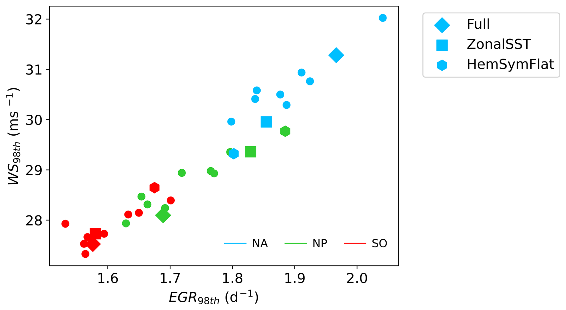
Figure 7 Scatterplot of winter basin-wide 98th percentiles of near-surface wind speed (y axis) vs. winter basin-wide 98th percentiles of mid-tropospheric Eady growth rates (x axis) across 11 different ISCA experiments with varying boundary conditions. Different colors represent different basins (same colors as in Figs. 1c, 5, and 6a), while shapes different than simple dots represent experiments chosen for the analysis. ERA5 values are shown in Fig. S3 in the Supplement.

It therefore appears that the changes in EGR between the experiments point to the characteristics of the basins which are responsible for their surface wind extremes. In more general terms, latent heat release helps to set the mean thermal structure of the troposphere, indirectly affecting EGR. This means that EGR implicitly and at least partly reflects the role of moist processes. For these reasons, we tie our analysis of basin-wide changes in extreme surface winds to changes in EGR and focus on the experiments where they differ the most from the Full experiment.

Zonalizing the SSTs has substantially larger influence on 98th-percentile surface winds in the NH basins than in the SH. This is not surprising, as the basins in the NH are bounded by the continents that, through warm boundary currents, influence SST distribution. However, the response of the NA differs from that of the NP. In the NA, zonalizing SSTs cools most of the NA storm tracks in a way which reduces both meridional and zonal temperature gradients. This is consistent with a weaker jet and decreased EGR in the center of the NA storm track, creating less favorable conditions for the development of extreme winds (see Fig. 8b, e, and h). The basin-wide decrease of EGR in the ZonalSST simulation mainly comes from decreases in the vertical wind shear.

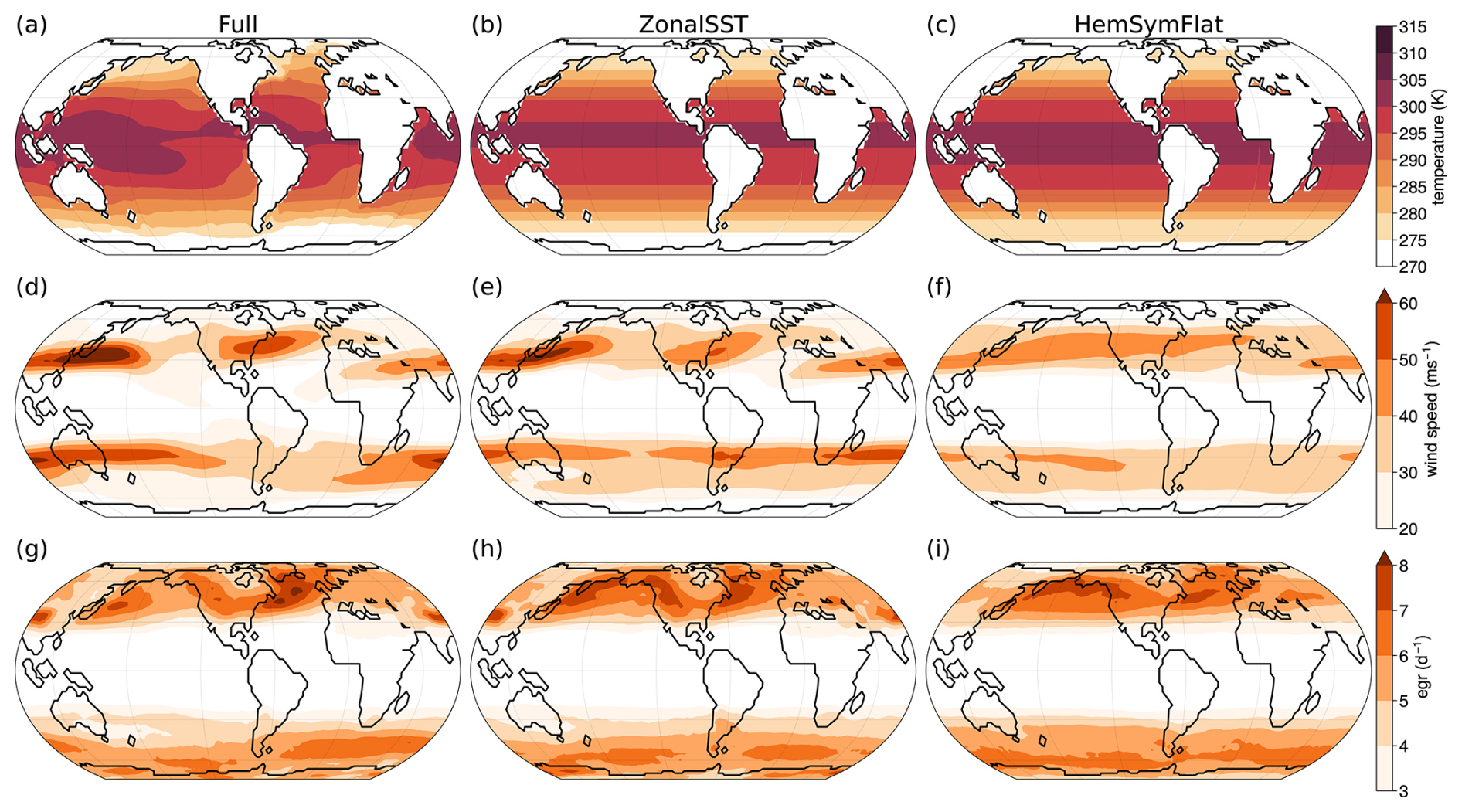
Figure 8 Climatologies of SSTs (a–c), medians of wind speed between 200–300 hPa (d–f), and EGR (g–i) during respective winter seasons across ISCA experiments. (a), (d), (g) show the results from Full, (b), (e), (h) ZonalSST, and (c), (f), (i) HemSymFlat experiments.

On the contrary, zonalization leads to increased SSTs across the NP storm track while warm regions of the tropical Pacific ocean cool (Fig. 8b). Therefore, the previously large meridional temperature gradient in the subtropical western Pacific is reduced, weakening the zonal component of the jet. As a result, the jet becomes more tilted and its orientation starts to resemble that of the NA jet (Fig. 8e). Basin-wide EGR in the NP storm track also increases – mainly as a result of an increase in the stability term, with a contribution from the shear term in some places (Fig. 8h). We conclude that the larger surface wind extremes in the NA than in the NP are mostly due to the differences in tropical and mid-latitudinal SST patterns between the basins.

However, zonalizing the SSTs is not enough to substantially reduce the interhemispheric asymmetry between extreme surface winds in the NA and the SO, which is reduced only in the HemSymFlat experiment. The rise in SO extreme winds in the HemSymFlat experiment compared with the Full experiment is consistent with an increase in EGR across the SO storm track (Fig. 8i). The increase in EGR is comprised of increases in both wind shear and stability terms, although the stability term plays a bigger role. The different SST configurations as compared to the Full experiment lead to a poleward shift of the regions with the strongest meridional temperature gradient and jet intensity (Fig. 8f). The jet also covers a broader region than in the Full and ZonalSST experiments (Fig. 8f). Following this, EGR increases across the whole SO storm track compared to both the Full and ZonalSST experiments. Basin-wide 98th percentiles of EGR and surface winds in the SO are also the largest in the HemSymFlat experiment, which subsequently reduces the interhemispheric asymmetry.

Finally, as the HemSymFlat experiment does not change SSTs in the NH relative to the ZonalSST experiment, the different response that occurs in the extreme EGR and surface winds in the NA and the NP can be primarily be attributed to the orography changes. Flat orography reduces the tilt of the jet and makes it more zonally symmetric in both basins in the NH (Fig. 8d–f). In the NP, this is displayed as a broadening of the area with high winds present in the Full experiment. Meanwhile, the jet in the NA looses its tilt and weakens, consistent with a significant decrease of EGR extremes in the central NA.

Inasmuch as ISCA shows a strong positive correlation between basin-wide extremes in EGR and near-surface winds across the storm tracks, we note that the evolution of ISCA's top 100 most extreme cyclones is not demonstrably connected with pre-existing cyclones. We find the top 100 extremes in the three selected ISCA experiments in the same way as in ERA5 (by applying Eq. 1) and track the cyclones by connecting the MSLP minima across time-steps (i.e. tracking as in Stanković et al., 2024). Although the composites of MSLP anomalies (shown in the Supplement) do show the presence of negative MSLP anomalies downstream of top 100 extremes in the Full experiment, these anomalies are weak, spatially limited and somewhat differently organized between the basins. Therefore, even though ISCA is able to reproduce the climatological correlation between extremes in EGR and near-surface winds, the evolution of the individual most extreme cyclones in ISCA differs from those in ERA5.

4 Summary and discussion

Our study shows that the presence of a pre-existing downstream cyclone is a distinguishing feature of cyclones associated with the top 100 extremes in surface winds in all storm track regions. Composite analysis shows that pre-existing downstream cyclones are accompanied by a strong jet and upper-level PV gradients, commonly observed in cyclones associated with extreme weather (e.g. Gómara et al., 2014; Messori and Caballero, 2015). Our results indicate that there is no qualitative difference in large-scale development of top 100 extremes across the North Atlantic, North Pacific and Southern Ocean storm tracks. Thus, our study generalizes the importance of pre-existing downstream cyclones in the development of cyclones associated with surface wind extremes across the hemispheres, previously documented for the North Atlantic (Stanković et al., 2024).

Quantitatively, however, the top 100 extremes differ across the hemispheres: specifically, in the NH they occur in the presence of stronger upper-level PV gradient, jet streak and mid-tropospheric EGR than the top 100 extremes in the SH. In addition, the percentage of top 100 extremes that develop explosively is almost two times higher in the NH. Clear differences in deepening rates help explain why surface wind extremes are stronger in the NH than in the SH (Stanković and Caballero, 2025). Simply put, a “large-scale recipe” for generating cyclones with the largest surface wind extremes is similar in all storm track regions. The recipe involves the presence of a pre-existing downstream cyclone situated poleward and eastward of an extreme-causing cyclone (as previously found for the North Atlantic in Stanković et al., 2024), whose deepening rate controls how large a surface wind extreme can be achieved. Higher rates of deepening in the NH can be linked to the higher mid-tropospheric EGR than in the SH. The EGR around top 100 extreme cyclones has its highest values around the jet streak, whose strengthening is tied to the presence of pre-existing downstream cyclones.

Simulations with ISCA further support using EGR for the purpose of analyzing surface wind extremes, as the basin-wide extreme values of EGR scale surprisingly well with the surface wind extremes across experiments. The extremes in the NA and the NP converge when extratropical and tropical SSTs are zonalized, and the interhemispheric asymmetry between the NA and the SO is reduced when extratropical and tropical SSTs are zonalized and orography is flattened. When SSTs are zonalized, the jet in the NA weakens while keeping its tilt, and extremes of surface wind and EGR weaken simultaneously. On the other hand, the jet in the NP becomes weaker, while attaining a tilt. In the NP, the new configuration of the jet happens together with the increase in the surface wind extremes, which climatologically become almost as strong as those in the NA (the NA-NP difference in extreme winds is reduced by ≈82 %). The jet core in the NP has climatologically higher values than the jet core in the NA in both ERA5 and ISCA, which could be an important ingredient driving NA-NP storm track differences. For example, Nakamura (1992) argued that a stronger jet core corresponds to more intense development of baroclinic wave activity up to a threshold, which the NP jet core often exceeds, after which a stronger jet core has the opposite effect. Therefore, it might not be surprising that an increase of extreme near-surface winds in the NP happens when its jet core is weaker. This argument is further explored by Hadas and Kaspi (2026), who propose that the larger tilt and weaker wind speeds of the NA jet allow for storms to grow longer there than in the NP, which eventually makes the storms stronger in the NA. Our ISCA experiments discussed above support this argument.

Our results show that the reduction of interhemispheric asymmetry in extreme surface winds between the NA and SO by ≈83 % with flat orography and zonalized, hemispherically symmetric SSTs happens through a decrease in extreme winds in the NA and an increase in the SO, consistent with an increase in EGR over the South Pacific. There are numerous studies that model the flattening of the Antarctic orography exploring a broad range of changes it causes in the SH circulation (e.g. Mechoso, 1980; Walsh et al., 2000; Singh et al., 2016; Patterson et al., 2020). Although there are differences in experiment set-ups between these studies and ours, the increase of extreme winds in the SO we observe could be tied to enhanced poleward energy and momentum transport by baroclinic eddies (Singh et al., 2016) and an increase in high-latitude eddy kinetic energy when the Antarctic orography is removed (Patterson et al., 2020). On the other hand, the further decrease (increase) in the zonalized SST experiment of the extreme winds over the NA (the NP) when the orography is flat shows that the orography also plays a role in shaping the extremes of the NH. The experiment with flat orography, however, exhibits non-linear effects on the NH storm track, as a decrease of extreme winds in the NA, for example, happens only with zonalized SSTs (flat orography and non-zonalized SSTs cause a slight increase in extreme winds over the NA). These results provide insight into how orography might influence NH near-surface wind extremes, thus complementing a vast body of previous work on disentangling the influence of orography on mean characteristics of large-scale circulation in the NH (e.g. Brayshaw et al., 2009; White et al., 2021; Shaw et al., 2022).

The fact that ISCA represents the climatological hemispheric asymmetry in extreme near-surface winds at a coarse resolution (T42) is another useful finding of our study. First, it points out that the hemispheric asymmetry is most likely primarily driven by large- and planetary-scale processes, as finer-scale processes are neither resolved at T42 resolution nor in ISCA's parametrization schemes. Second, documenting the asymmetry at a low resolution with simple parametrizations is a first natural step in studying this phenomenon across a hierarchy of climate models. Moving to more complex models could provide further insights into the hemispheric asymmetry and dynamics of the extreme cyclones by enabling step-wise investigation of processes at increasingly small scales.

It is worth noting some of the limitations of our results. Our focus on the large scales means we do not consider mesoscale or boundary-layer processes which can play an important complementary role in generating surface wind extremes (Hewson and Neu, 2015). In addition, the most prominent feature for the top 100 extremes is the presence of a pre-existing downstream cyclone. Our results mainly focused on the role of this pre-existing cyclone in generating a large-scale environment suitable for development of top 100 extremes, without considering the merging and cyclone-cyclone interaction between extreme and pre-existing cyclones. Further, although the ISCA model is able to represent the main features of the Earth's climate relevant for our study (like PDFs of surface winds in the storm track regions), it does not fully capture the presence of pre-existing downstream cyclones in the evolution of individual cyclones associated with extreme winds. Assessing whether ISCA run at a higher resolution could better represent cyclone-cyclone interactions in top extremes as documented in ERA5 is a potential avenue for future research. ISCA also has some known biases relevant to storm track behavior. For example, like many other climate models (Shaw et al., 2016; Patterson et al., 2020), it has a jet that is too zonal and located more equatorward than in the observations. Finally, ISCA does not have a realistic representation of clouds, which possibly limits an extension of our analysis to project the changes in the storm track with anthropogenic warming, as biases in cloud representation are one of the main uncertainty sources relevant for storm tracks (Shaw et al., 2016).

Finally, there are approaches that can be applied to extend the results from our study. The study could be complemented by the inclusion of other extremes, like precipitation extremes, that often accompany cyclones that cause extreme winds (Pfahl and Sprenger, 2016; Cornér et al., 2025). Although less frequently, some extreme surface winds associated with cyclones happen outside winter seasons (especially in the SH, e.g. Stanković and Caballero, 2025) and an analysis of large-scale characteristics of cyclones in seasons other than winter could generalize the understanding of cyclones that cause extreme surface winds. When it comes to modeling, a next step could be to test whether one of our main results that extreme basin-wide EGR scales with the extreme surface winds holds in more complex, coupled climate models or in climates that greatly differ from the present one. Other approaches, like those applying energetic frameworks, are better suited than EGR-like metrics to represent mean storm track activity in climates of snowball Earth (Shaw and Graham, 2020) or with an intense warming (Shaw et al., 2018). It could be beneficial to contrast usefulness of these zonal-mean metrics in representing surface wind extremes with our analysis focused on basin-wide metrics. Examining how the cyclones that cause surface wind extremes would change with projected future climates could employ the use of models with high resolution (like for e.g. Gentile et al., 2023, 2025), focus on compound extremes related to explosively deepening cyclones (e.g. Lopez-Marti et al., 2025) or leverage understanding that comes from idealized climate simulations (e.g. Sinclair and Catto, 2023; Bouvier et al., 2025).

5 Conclusions

In this study, we analyze historical extratropical cyclones associated with the 100 most extreme surface winds over the North Atlantic, North Pacific and Southern Ocean storm tracks. Our study is motivated by the observation that such surface wind extremes are more intense in the NH, and in particular in the North Atlantic, than in the SH. We employ composite analysis to study the large-scale features of the flow around these cyclones and we perform modeling experiments to examine differences in characteristics of the storm track basins relevant for surface wind extremes. Finally, we answer the questions posed in the Introduction as follows:

1. The presence of a pre-existing downstream cyclone is a key large-scale feature of the development of cyclones associated with the top 100 most extreme surface winds in all storm track basins. Pre-existing cyclones are situated poleward and eastward of developing top 100 extremes and they intensify strong jet streaks and upper-level potential vorticity gradients within which the top 100 extremes develop. After crossing the jet streak, at the time of the maximum surface wind severity, the top 100 extremes merge with pre-existing downstream cyclones to form a large area of negative mean sea-level pressure anomalies.

2. Large-scale differences between the basins are quantitative. Though composite analysis shows qualitatively similar development of the top 100 extremes in different basins, those in the Northern Hemisphere deepen more explosively and are surrounded by higher values of mid-tropospheric Eady growth rates. The highest values of Eady growth rates are primarily found around the jet streaks, which are stronger in the Northern Hemisphere where surface wind extremes are higher.

3. Idealized modeling experiments with different boundary conditions show a strong positive correlation between basin-wide extreme surface winds and basin-wide extreme Eady growth rates. The North Atlantic has the highest extreme winds and Eady growth rates, but they become almost equal to those in the North Pacific when inter-basin sea-surface temperature differences are removed by zonalizing them across the tropics and extratropics. On the other hand, the interhemispheric asymmetry in extreme surface winds between the North Atlantic and the Southern Ocean is greatly reduced once sea-surface temperatures are zonalized, made hemispherically symmetric and the orography is flattened.