Quantifying atmospheric and land drivers of hot temperature extremes through explainable Artificial Intelligence

Different drivers have been shown to play a central role in modulating the occurrence and intensity of summer temperature extremes, yet their individual contributions remain difficult to quantify. In this study, we develop an explainable machine‐learning framework to disentangle the respective influences of large‐scale atmospheric circulation, soil‐moisture anomalies, and rising CO₂ concentrations on boreal‐summer temperature extremes at six locations across Europe and North Africa with different characteristics of land–atmosphere coupling (Córdoba, Lyon, Hannover, Stockholm, Belgrade, and Marrakech). Using SHapley Additive exPlanation (SHAP) values, we find that the atmospheric circulation consistently dominates model explainability across all locations, contributing to 66 %–86 % of the total mean SHAP, with the geopotential at 500 hPa field contributing the most. Soil‐moisture influence exhibits a northward gradient: negligible at Marrakech (0.2 %), moderate at Córdoba (9.4 %), and substantial at Lyon (15.4 %). Additionally, the dominant shallow soil-moisture signal shows an inverse relationship between moisture anomalies and SHAP values, consistent with the amplifying effect of land drying on heat extremes, while attribution for deeper layers is weaker and less robust across locations. We demonstrate the robustness of these findings to a less stringent (80th percentile) extreme definition. Furthermore, the identified driver contributions are consistent when using alternative observational data for temperature extreme definition and for computing SPI/SPEI drought indices as proxies for soil moisture, with SPEI showing a closer alignment to the original ERA5-Land results. We also illustrate the methodology for case studies of two individual events, heatwaves occurring in Córdoba (Spain) 2021 and Hannover (Germany) 2018, which reveal a pronounced spatial pattern in the distribution of SHAP values for the circulation predictors. They also confirm the enhanced role of the land component in regions of Northern Europe and reveal a contribution of the anthropogenic factor through CO₂ concentrations, even for specific events. These results align with the established physical roles of atmospheric circulation and soil moisture modulation for temperature extremes, and demonstrate the methodological potential of explainable artificial intelligence to quantify the relative contributions of these drivers in a data-driven framework.

1 Introduction

Understanding weather extremes is of vital importance due to their impacts on society and ecosystems. Events such as extreme precipitation, severe droughts, and intense heatwaves pose growing threats to biodiversity and sectors like agriculture, energy, health or the economy (e.g., Zscheischler et al., 2018). As the climate warms, evidence from observations and model simulations shows that these events are becoming longer, more intense and more frequent (Intergovernmental Panel On Climate Change, 2023). Consequently, predicting, characterizing, and understanding these events is crucial for the development of early-warning systems and adaptation strategies in a climate change context.

Much progress has been made in identifying the physical processes driving temperature extremes, although many mechanisms are still not well understood due to difficulties in quantifying their interactions and responses to climate change (Barriopedro et al., 2023). The changing behaviour linked to the positive trends in global temperatures poses challenges for establishing a unique definition or common metrics describing hot extremes (Perkins and Alexander, 2013).

Hot extremes are primarily driven by a combination of atmospheric, ocean, and land surface conditions, including persistent high-pressure systems and soil moisture deficits (Barriopedro et al., 2023). In this study, we discard the ocean drivers because we are focusing on the short term variability drivers of hot extremes. Additionally, we include atmospheric CO₂ concentrations to capture the multiyear trend of hot extreme events. Many studies focus on understanding the role of these land–atmosphere interactions, such as the positive soil-moisture–temperature feedback, and its amplification role during high-pressure conditions (Materia et al., 2022; Quesada et al., 2012). This amplification becomes especially relevant in a changing climate due to the evidence of regional shifts of wet, dry and transitional evaporative regimes (Hsu and Dirmeyer, 2023). Seneviratne et al. (2006), for instance, highlight the need of including land–atmosphere interactions in regional simulations to correctly modulate the increase in summer temperature variability (and resulting temperature extremes) in central and Eastern Europe due to increasing greenhouse gas concentrations.

Regarding the role of the atmospheric circulation, many studies show the direct link of hot extremes to atmospheric circulation patterns, such as persistent double jets over Eurasia (Rousi et al., 2022), mid-tropospheric deep depressions over the North–Atlantic (D'Andrea et al., 2024), or episodes of Saharan warm air intrusion in the West Mediterranean (Cos et al., 2025).

In addition, growing attention is being paid to heatwave-driving mechanisms related to other elements of the Earth system, like particular patterns in preceding sea surface temperatures identified as precursors of summer heatwaves in Europe (Beobide‐Arsuaga et al., 2023).

Complementing physical understanding, new tools and methodologies are being actively explored to improve the identification and prediction of temperature extremes. In particular, Artificial Intelligence (AI) and Machine Learning (ML) approaches are emerging as powerful complements to traditional numerical modelling techniques (Camps-Valls et al., 2025). Moreover, ongoing developments in explainable AI (XAI) offer promising pathways to interpret model behaviour, allowing researchers to assess the contribution of individual drivers to extreme events (Materia et al., 2024). This capability is critical not only for attribution purposes, but also for potentially gaining new insights into the underlying physical mechanisms.

For example, Toms et al. (2020) demonstrate how explainable ML methods such as layerwise relevance propagation (LRP) and backward optimization can be used to interpret neural network predictions in climate applications, revealing scientifically meaningful relationships between input patterns and network outputs. Davenport and Diffenbaugh (2021) employ LRP to analyse large-scale circulation patterns associated with extreme precipitation. Other explainable AI (XAI) techniques such as SHAP have also been used to assess the relative importance of different climate drivers; for instance, Uckan et al. (2025) apply SHAP values within a Random Forest framework to quantify the contribution of multiple heatwave drivers at the global scale.

In this study, we aim to disentangle the respective roles of atmospheric circulation, soil moisture and anthropogenic climate change in driving extreme temperature events during the boreal summer (JJA), using an explainable ML modelling framework. With this goal in mind, we aim to develop a framework that is both predictive and diagnostic.

First, we classify daily extreme events using the 90th percentile threshold of the climatological maximum temperature distribution. Then, we build a robust extreme/no-extreme binary classifier using supervised ML, with lagged anomalies of large-scale circulation variables and soil moisture, and atmospheric CO₂ concentrations as inputs. To understand the drivers learned by the ML model during the prediction task, we apply the SHAP explainability technique to quantify the contribution of each input feature to the model's predictions (Lundberg and Lee, 2017a). First, we compute general aggregated SHAP values for each variable to obtain a general characterization of feature relevance. Then, we proceed by analysing specific SHAP explanations for two case studies to investigate region-specific driver behaviour: the August 2021 heatwave in Córdoba and the July 2018 heatwave in Hannover. These events were selected to represent contrasting soil-moisture feedback regimes – dry/transitional versus transitional/wet – with differing soil moisture variability and land-atmosphere coupling strengths (Hsu and Dirmeyer, 2023). We extend our explainable ML analysis to evaluate the robustness of our driver attribution to different extreme thresholds (80th and 95th percentiles) and to the use of alternative observational data for the extreme event classification and the land component features.

In Sect. 2 we discuss the data and methodology, including the datasets used, the domain for circulation data, the selected locations based on different soil-moisture feedback regimes, the deep learning model used and the explainability method. In Sect. 3 we show and discuss the results: we display the extreme classification results, give a statistical assessment of the model, and provide the SHAP explainability results. Lastly, conclusions of the study can be found in Sect. 4.

2 Data and methodology

2.1 Datasets

We use data from ERA5 (Hersbach et al., 2020; Soci et al., 2024), the fifth-generation atmospheric reanalysis from the European Center for Medium-Range Weather Forecasts (ECMWF), which provides globally complete, gridded data from 1940 to the present. The long-term availability and spatial completeness of reanalyses make them suitable for studying climate trends, variability, or extreme events despite substantial uncertainties across datasets (Donat et al., 2014). We use daily data using the spatial domain discussed in Sect. 2.3. We use atmospheric circulation fields that represent the state of the atmosphere and constitute the large-scale variables in the study: Geopotential at 500 hPa (g500) [m² s⁻²], Geopotential at 200 hPa (g200) [m² s⁻²], and Sea Level Pressure (psl) [hPa].

For land-surface variables, we use the ERA5-Land dataset. Soil moisture variability is more consistent in ERA5-Land because it does not assimilate screen-level observations to adjust soil moisture (unlike the ERA5 reanalysis) (Muñoz-Sabater et al., 2021). The variables we use are daily maximum 2 m temperature (TX) to define our target events, and soil moisture at three depth levels (swvl1, swvl2, and swvl3) as predictors. TX from ERA5-Land is only used to define hot extremes, as the prediction target of the ML model. All land-surface variables are taken as the spatial average over a 100 km × 100 km region to avoid focusing on a single grid-point.

Lastly, we include seasonal atmospheric CO₂ concentrations to account for the trend of climate change. We employ U.S. National Oceanic and Atmospheric Administration (NOAA) measurements collected at the Mauna Loa Observatory in Hawaii. The concentrations used have a constant value for each summer and are a seasonal mean. By explicitly including CO₂, our framework controls for the long-term warming trend as a potential additional driver of heat extremes, allowing for a cleaner attribution of the physical drivers.

Circulation and land variables are used as lagged standardized anomalies (explained in Sect. 2.4). For each prediction day, the model is trained on features derived from values recorded on preceding days. For the local-scale, soil moisture is averaged over the previous 7 d to account for its relatively low daily variability (Miloshevich et al., 2023). The values of circulation variables are taken from the day before the prediction, corresponding to a 1 d lag in atmospheric features. The inclusion of up to three lags for the circulation features was tested, but we decided to keep a simpler model because the accuracy did not improve by including more lags (not shown).

Similar variable sets using atmospheric circulation and land features have been used in Koh et al. (2025), where they developed a machine-learning framework combining spatial extreme-value theory and adapted loss functions to study large-scale heat extremes, or in Miloshevich et al. (2023), who predict the probability of occurrence of long-lasting 14 d heatwaves over France.

2.2 Observational data and drought indices

To test the robustness of our results to the data source, we supplement the analysis based on reanalysis with observational data for the daily maximum temperature and the land component. For the atmospheric circulation features, we keep the data from ERA5. For the local-scale daily maximum temperature used in the extreme event definition, we use directly the E-OBS gridded dataset (version 29.0) of TX (Cornes et al., 2018).

Due to the lack of long-term, consistent observational soil moisture records, we employ the Standardized Precipitation Index (SPI) (McKee et al., 1993) and the Standardized Precipitation Evapotranspiration Index (SPEI) (Vicente-Serrano et al., 2010) as proxies for soil moisture anomalies, computed with the E-OBS data. These indices serve to validate the robustness of our ERA5-Land results against observational data, providing a reliable alternative for historical comparison. These indicators have already been assessed as surrogates of in situ and satellite soil moisture observations (Scaini et al., 2015; Wang et al., 2015; Yuan et al., 2020), with generally larger association when potential evapotranspiration is included. We use the Hargreaves method (Masmoudi-Charfi and Habaieb, 2014) for computing the evapotranspiration, essential for the SPEI calculation, and the gamma distribution to standardize the data. Precipitation and temperature data are sourced from the E-OBS dataset. As for soil moisture, both SPI and SPEI grid-points are averaged spatially over a 100 km × 100 km region.

The timescale for the index computation was selected by computing the Spearman correlation of the drought indices with the three soil moisture levels of the original model (see Figs. C1 and C2). Soil moisture is a variable with a memory that extends beyond a few days (Vicente-Serrano et al., 2010), so the drought index must be computed on a scale that reflects this persistence. Based on the correlation analysis, the selected timescale for the SPEI and SPI indices is 30 d (SPEI30d and SPI30d). This timescale shows the best correlation of the indices with swvl1 and swvl2, which we show to be in general the most relevant depth levels in our explainability analysis (see Sect. 3). We also computed the correlation using a 7 d rolling mean of the soil moisture data – the same preprocessing applied before inputting soil moisture to the model – and obtained very similar results, with correlation values not differing more than 0.07. Additionally, we computed the drought indices using ERA5 data to validate the correlations computed with the E-OBS gridded data, with correlation between datasets not differing more than 0.1. In the correlation analysis, we did not lower the timescale of the drought indices computation (e.g. 15 d) to stay within the original monthly definition of the indices (Vicente-Serrano et al., 2010), and to avoid fitting the normalized distribution to data that may not be sufficiently smooth.

2.3 Atmosphere data domain and target locations

With the atmospheric pressure and geopotential height fields, we aim to capture the general circulation influencing the locations where we predict extreme temperature events. The large-scale domain must be large enough to cover the area of interest, but not too large to avoid including unrelated atmospheric variability (Mahlstein et al., 2015). Figure 1 shows the selected domain marked as a red box. The full North Atlantic Ocean is included, since studies link this region to the development of extreme temperature events in various European regions (Bischof et al., 2023). A large part of North Africa is included as well to capture warm and dry intrusions that may enhance the likelihood of extremes (Cos et al., 2025). The northern and eastern limits are extended enough to include synoptic-scale circulation patterns.

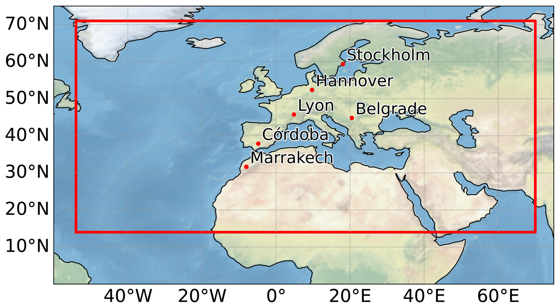
Figure 1 Large-scale data domain and locations selected for the local-scale data in the prediction target. The red box indicates the domain used in the study for the ERA5 data, with longitudes ranging from 54° W to 70° E and latitudes from 14 to 71° N. Locations are illustrative for different climate regimes in Europe.

We study the roles of circulation, soil moisture and anthropogenic climate change during extreme temperature events in six regions around Córdoba, Marrakech, Lyon, Belgrade, Hannover, and Stockholm (see Fig. 1). For each site, local-scale data is averaged over a surrounding 100 km × 100 km region, to smooth out unwanted variations across space. The chosen locations span different evaporative regimes: from water-limited (Marrakech) to energy-limited (Stockholm). Location choice is also partly based on literature: Córdoba and Marrakech are studied in Lemus-Canovas et al. (2024), Stockholm's 2018 heatwave in Wilcke et al. (2020), and Iberia and Central Europe heatwaves in Khodayar Pardo and Paredes-Fortuny (2024). Belgrade was selected to provide a more eastern perspective, potentially influenced by sea surface temperatures and atmospheric anomalies in other regions discussed in Beobide‐Arsuaga et al. (2023).

Lastly, the robustness analysis using observational data (discussed in Sect. 2.2) could not be carried out for Marrakech, due to missing data for several years (see Fig. 4).

2.4 Climatology, anomalies and the extreme temperature definition

Both the climatology and 90th percentile are computed only for the reference period 1950–2000, within the model's training period (1950–2014). This avoids an indirect provision of future information to the model, which would leak evaluation data into training. The training period was extended to 2014 to include a period with a clear trend in the yearly count of extremes (see Fig. 4).

First, we calculate the raw climatology by taking the daily average. Then, as in Mahlstein et al. (2015), we apply a local polynomial regression (LOESS) to obtain a smoothed profile. After a few tests with the window timescale, we selected a 30 d smoothing window for both climatology and standard deviation. Anomalies are computed daily by subtracting the smoothed climatology from the original data, and then standardized using the standard deviation. Subtracting the climatology removes the annual cycle, and applying the LOESS smoothing removes the short-term variability (see Fig. 2 example for Córdoba site). Extended detail on LOESS is given in Appendix A1.

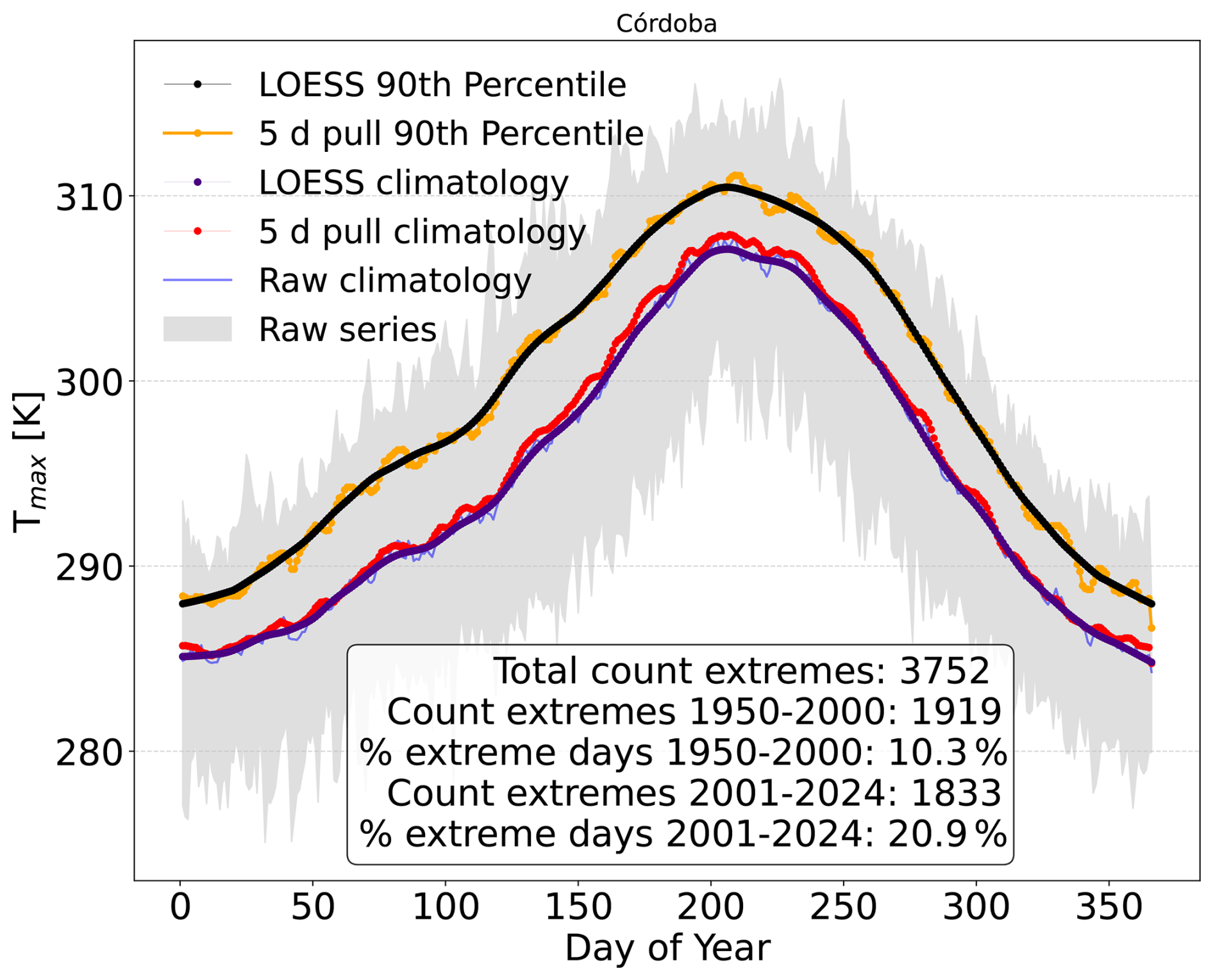
Figure 2 Climatology and percentiles for the region of Córdoba. Day of the year (x-axis) and daily maximum 2 m temperature from ERA5-Land (y-axis). We show the raw climatology and percentiles, together with the 5 d window pull and LOESS smoothing versions. The text box shows the total frequency of heat wave events, and the separated frequencies for the reference period 1950–2000, and the rest of the time series (2001–2024).

Using the extreme definition in Perkins and Alexander (2013) an extreme event is defined when the daily mean maximum temperature exceeds a specified percentile of the climatological distribution. Following Beobide‐Arsuaga et al. (2023), the percentile is calculated over a centered 5 d window using the reference period, and then we apply LOESS smoothing with a 30 d window. We use a 5 d rolling window prior to the LOESS smoothing to increase the number of samples available for estimating the 90th percentile for each calendar day. The window is centered in the day for which the percentile is computed. The primary analysis in this study uses the 90th percentile, but to test the robustness of our results to the extreme event definition, we conduct additional analyses using the 80th and 95th percentiles, and all are computed following the same procedure.

2.5 The deep learning model

The model is trained on data from 1950 to 2013. Validation years are chosen by randomly selecting contiguous blocks of years (see Table B1), while the testing period spans 2014 to 2024. Extreme days are defined using the 90th percentile threshold (i.e., approximately 10 % of all days), which results in a class imbalance between extreme and non-extreme days (see Table B1). This imbalance represents a central challenge during model training, as machine learning algorithms may default to predicting the majority (non-extreme) class if no specific strategy is used to address it. At the same time, the relatively limited number of extreme cases increases the risk of overfitting in this binary classification problem when using models with many parameters. This constraint needs to be considered when designing the model architecture and training procedure. The imbalance issue becomes even more pronounced when higher percentile thresholds are used to define extremes, as the number of available training samples decreases further. (see Table B1). In this study, we treat the class imbalance by training the model with a weighted loss function. By doing this, we penalize more the wrongly classified extreme samples.

The main contributor to high parameter dimensionality are the large-scale fields, which include spatial dimensions at 0.25° resolution, unlike local-scale data that is area-averaged and provides time-only vectors. Flattening large-scale data would result in $n_{\mathrm{var}}\cdot n_{\mathrm{lags}}\cdot n_{\mathrm{lat}}\cdot n_{\mathrm{lon}}$ inputs, making the model overly complex. We first reduce dimensionality by re-gridding large-scale data to 1°, directly reducing computational cost and overfitting risk. We think this coarser resolution still captures atmospheric circulation features for extreme temperatures.

We use a model architecture designed to capture land–atmosphere coupling (see Fig. 3). It includes a Multi Layer Perceptron (MLP) for land and CO₂ data, and a ConvNeXt convolutional neural network (CNN) (Liu et al., 2022) for spatial features from circulation, which, to our knowledge, has not been used before in driver quantification studies. Their outputs are concatenated and passed to a final MLP for binary classification of extreme or non-extreme on a daily basis. This architecture is hereafter referred to as the CombinedModel.

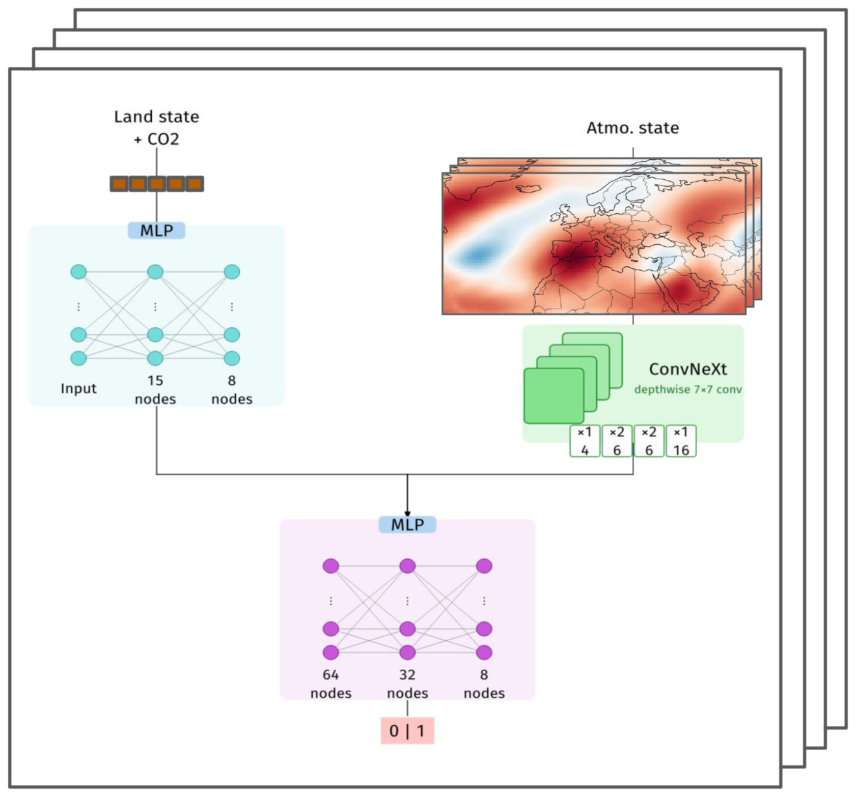
Figure 3 Diagram of the Combined Model. Includes a simple MLP for the Land-State plus a ConvNeXt model for the Atmosphere state, which are then combined using a final MLP that does the binary classification. An ensemble of 20 members is used during training to add robustness and treat the model's epistemic uncertainty.

The MLP for the Land State + CO₂ inputs receives an input vector of dimension d_in, followed by two hidden layers of 15 and 8 nodes. The final classification MLP then takes the concatenated outputs from the Local and Large-scale branches (with dimensions 8 and 16, respectively) as its input. These features are processed through three hidden layers of 64, 32, and 8 nodes before reaching the final output layer. For the spatial feature extraction, a custom ConvNeXt architecture is employed. The model accepts input tensors with C channels (corresponding to the number of Large Scale features) and utilizes a patch size of 4. The ConvNeXt here consists of four stages with depths of $[\mathrm{1},\mathrm{2},\mathrm{2},\mathrm{1}]$ and corresponding layer dimensions (channels) of $[\mathrm{4},\mathrm{6},\mathrm{6},\mathrm{16}]$. A dropout rate of 0.05 is applied to prevent overfitting during training. The architecture of the ConvNeXt model is explained in detail in Liu et al. (2022). ReLU is used as activation function in the MLPs, and softmax applied at the output to yield probabilities (Goodfellow et al., 2016). A 0.5 threshold determines the predicted class, kept constant throughout the study. Additionally, we use a 20-member ensemble to filter out noise and handle part of the epistemic uncertainty of the model. These ensembles are generated by changing the initial random seed (detailed in Sect. 2.7). Similar hybrid model architectures have been used in the past (Gordon et al., 2023; Mayer et al., 2024).

The optimizer used for the CombinedModel is the AdamW optimizer (Loshchilov and Hutter, 2019). We train the model with an 80 % and 20 % random split of the samples for the training and validation respectively, and apply a random shuffle. The Cross-Entropy Loss function is used (see Sect. A2), with specific weights applied to the non-extreme and extreme classes to address the class imbalance. The Optuna Python package is used for the tuning of the following hyperparameters of the ML model: batch size, learning rate, weight decay and class weights of the predicted classes. The model is trained for 75 epochs unless validation loss increases for a total of five epochs. The score used in the hyperparameter tuning process is the balanced accuracy minus the final validation loss, which is the best validation loss found before early-stopping.

2.6 Explainability of the machine learning model using SHapley Additive exPlanation values

To quantify the contribution of each input feature to the model's predictions, we use SHapley Additive exPlanations (SHAP), a game-theoretic approach that explains the output of any machine learning model by attributing it to the input features (Lundberg and Lee, 2017a).

Positive SHAP values mean a positive influence on the likelihood of the predicted class by the model, while a negative SHAP value means that the feature decreases the likelihood of predicting the class. The magnitude of the value quantifies the influence of the feature, and SHAP values are zero for irrelevant. SHAP values are an additive feature attribution method, meaning that the contribution of each feature can be computed independently, and all values summed up.

The sum of the SHAP values across all features equals the model output (prediction) minus the expected (baseline) prediction:

$$\begin{array}{}\text{(1)}& f\left(x\right)={\mathit{\varphi }}_{\mathrm{0}}+\sum _i^N{\mathit{\varphi }}_i,\end{array}$$

where f(x) is the model prediction for the input x, ϕ₀ is the baseline (computed by averaging the model prediction over training and validation data), ϕ_i is the SHAP value for the feature i and N is the total number of features in the model. The additive nature of SHAP values allows us to compute a value per grid-point, highlighting the regions the model finds most important, and to spatially aggregate these values into global importance or combine them across features, as we do in Sect. 3.2.

We compute SHAP values in the testing period (years 2014–2024) using GradientExplainer (Lundberg and Lee, 2017b), which is designed for differentiable models, such as deep neural networks, and estimates them by using an extension of the integrated gradients method (Sundararajan et al., 2017). We believe this choice to be appropriate given the evaluation metrics results for the Integrated Gradients method shown in Bommer et al. (2024), though no XAI method evaluation was carried out for our study. Additionally, the method requires selecting a baseline to serve as a reference in the SHAP computation. Following best practices suggested by Mamalakis et al. (2023a), the baseline was constructed by selecting the samples from the training and validation period that had non-extreme labels. Using only non-extreme days for the baseline is appropriate in this study, as our focus is on identifying the drivers of predicted extreme events with the aforementioned ML model.

2.7 Creating robust explanations

Since our focus is to study the contribution of the atmospheric circulation, the soil moisture, and atmospheric CO₂ concentrations during extreme temperature events, we want to ensure that our explanations are done for predictions for which our model is confident. To do so, we take an ensemble of trained models with twenty members, adding robustness to our output probabilities and computed SHAP values. The members are created by setting deterministically twenty different seeds, initializing the random processes present in the framework. On top of that, we analyse the general explainability results for a certain percentage of top most confident predictions, following the approach of studies like Mayer and Barnes (2021).

We assess model performance using balanced accuracy (BA) and the Area Under the Receiver Operating Characteristic Curve (AUC), which are well-suited for imbalanced classification tasks.

3 Results and discussion

Figure 4 shows the yearly count of summer extremes (true labels) for the six selected locations, resulting from the extreme definition given in Sect. 2.4. We show the results of the extreme classification both for the ERA5-Land and E-OBS datasets. Clear warming trends are apparent for Córdoba and Lyon regions. Belgrade region also shows a visible trend after approximately 1960. To quantify these observations, we performed a formal linear trend analysis across different time windows (see Fig. B1). A generalized acceleration in the frequency of extremes is visible when comparing the full record against the period starting in 1980. In the most recent period (since 2000), a slight decrease in the trend magnitude – and a corresponding loss of statistical significance – is observed in Lyon, Marrakech, and Belgrade. A similar slight decrease in magnitude is noted for Córdoba when compared to the 1990–onwards period, though the trend there remains statistically significant. The average count during summer for the period 1950–2000 is approximately 10 for all locations, which is expected considering our 90th percentile definition of extreme. When comparing the classification results for ERA5-Land and E-OBS datasets, we see a general agreement except for some periods and locations like the 1950s decade in Córdoba, or the years 1950 and 1952 in Belgrade.

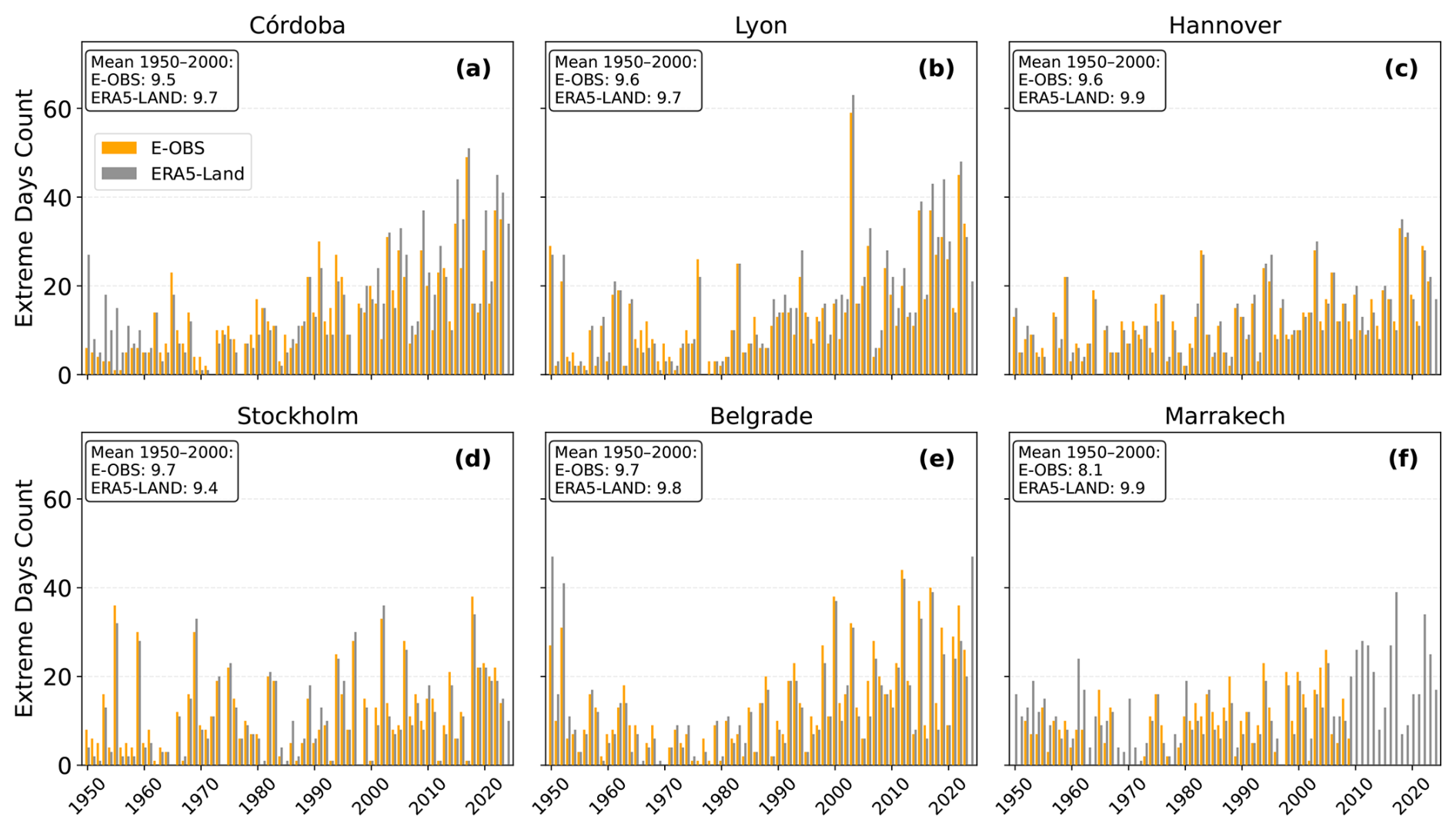
Figure 4 Extremes yearly count for the six locations for both ERA5-Land and E-OBS data. Yearly extreme count for the full period of used data in ERA5 and (1950–2024) E-OBS (1950–2023 for E-OBS). Years in the x-axis and count (number of extreme days) in the y-axis. The text box shows the mean count for the period 1950–2000 to verify the percentile definition of extreme in both datasets.

3.1 Prediction and statistical assessment of the models

For the primary analysis using the 90th percentile threshold (see Table 1) gives relevant statistics of the trained CombinedModel on the test data using the 50 % most confident predictions. Figure B2 shows how we assess the CombinedModel model robustness by plotting the evolution of accuracies when varying the confidence threshold. For each member individually, the CombinedModel shows a smooth increase in both balanced and extreme accuracy across all locations. The improvement in both accuracy measures with increasing network confidence is an expected behavior. For some locations, low percentages of confidence (see Fig. B2) show a trade-off between extreme and non-extreme accuracies, with the former increasing and the latter decreasing, until a minimum is reached and non-extreme accuracy starts improving again. We did not explore this behaviour in depth, but it may be related to how we handle class imbalance.

Table 1 Statistical assessment of the CombinedModel for the different locations, considering the 50 % most confident predictions. For the test data, we show the extreme class accuracy (EA), the non-extreme class accuracy (NEA), and the balanced accuracy (BA), which accounts for false positives and false negatives. TP, FP, TN, and FN stand for true positives, false positives, true negatives, and false negatives respectively. The last column shows the area under the ROC curve (AUC).

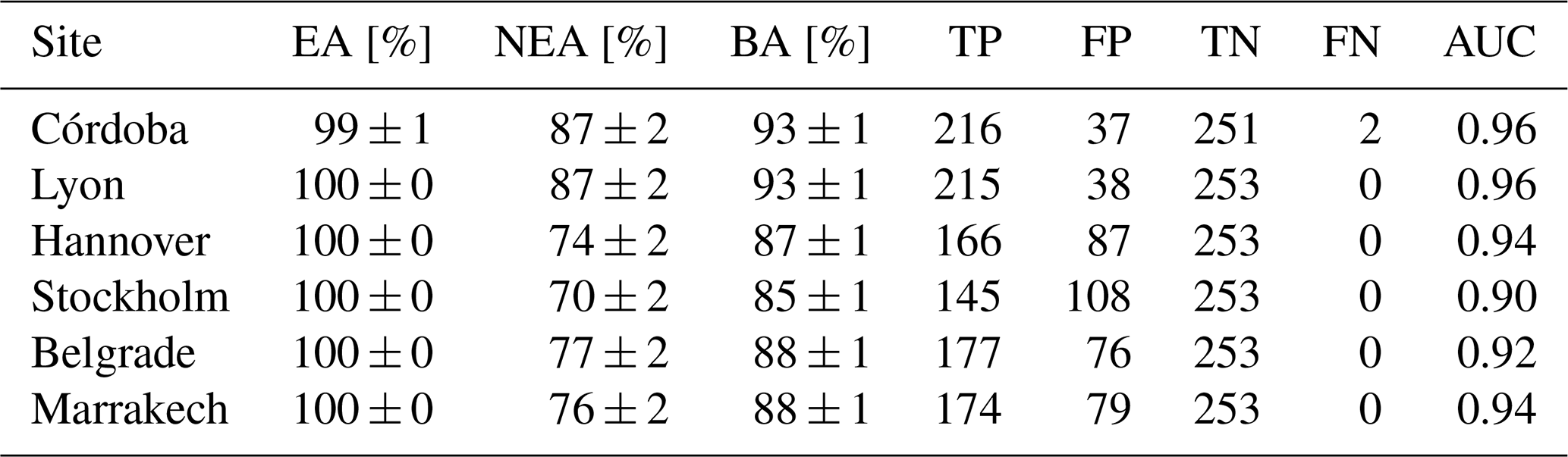
In Fig. B3 we show the ROC curve change when changing the percentage of confidence. When using the ensemble of 20 members, most locations show a displacement towards area under the ROC curve equal to 1.

The model trained on the 80th percentile definition shows a similar statistical robustness for the accuracies and ROC curves (Fig. B4). The increased number of extreme events mitigates class imbalance, resulting in smooth and consistent improvements in balanced accuracy and AUC values as the confidence threshold increases. This indicates the model is well-trained, and its predictions are reliable for this definition. In contrast, the model performance for the 95th percentile definition is notably weaker for most locations, with the balanced accuracy behaving poorly when increasing the percentage of confidence in the predictions. The drastically reduced number of extreme events (see Table 1) presents a significant challenge for training, leading to less stable behavior in accuracy metrics and ROC curves due to the strong class imbalance (see Fig. B5). The class imbalance and lack of extreme events samples is a known issue in ML application for weather extremes (Miloshevich et al., 2023; Sha et al., 2025), so the results using the 95th percentile are not surprising. Due to this lack of robust predictive skill, we do not consider the explainability results for the 95th percentile definition to be trustworthy.

Finally, the model trained with observational TX and SPI/SPEI indices for the 90th percentile also demonstrates robust predictive performance, providing confidence in the reliability of its explanatory outputs (not shown).

3.2 SHAP values

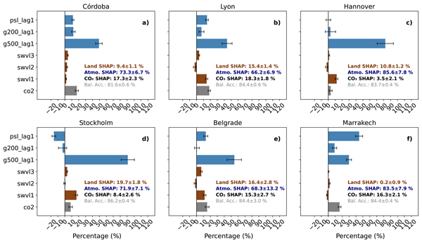
Taking the 50 % most confident extreme predictions, Fig. 5 shows the mean SHAP values across samples in the test dataset for each of the features in the model. The results are not sensitive to the confidence threshold. We calculate a global SHAP value for the Land and Atmosphere compounds by summing the contributions of their respective features, which can be done thanks to SHAP values being an additive feature attribution method. To determine the SHAP percentage for a feature, we first calculate the mean of its absolute SHAP values over the entire time series. This time-averaged mean is then expressed as a percentage of the total mean SHAP value contributed by all features.

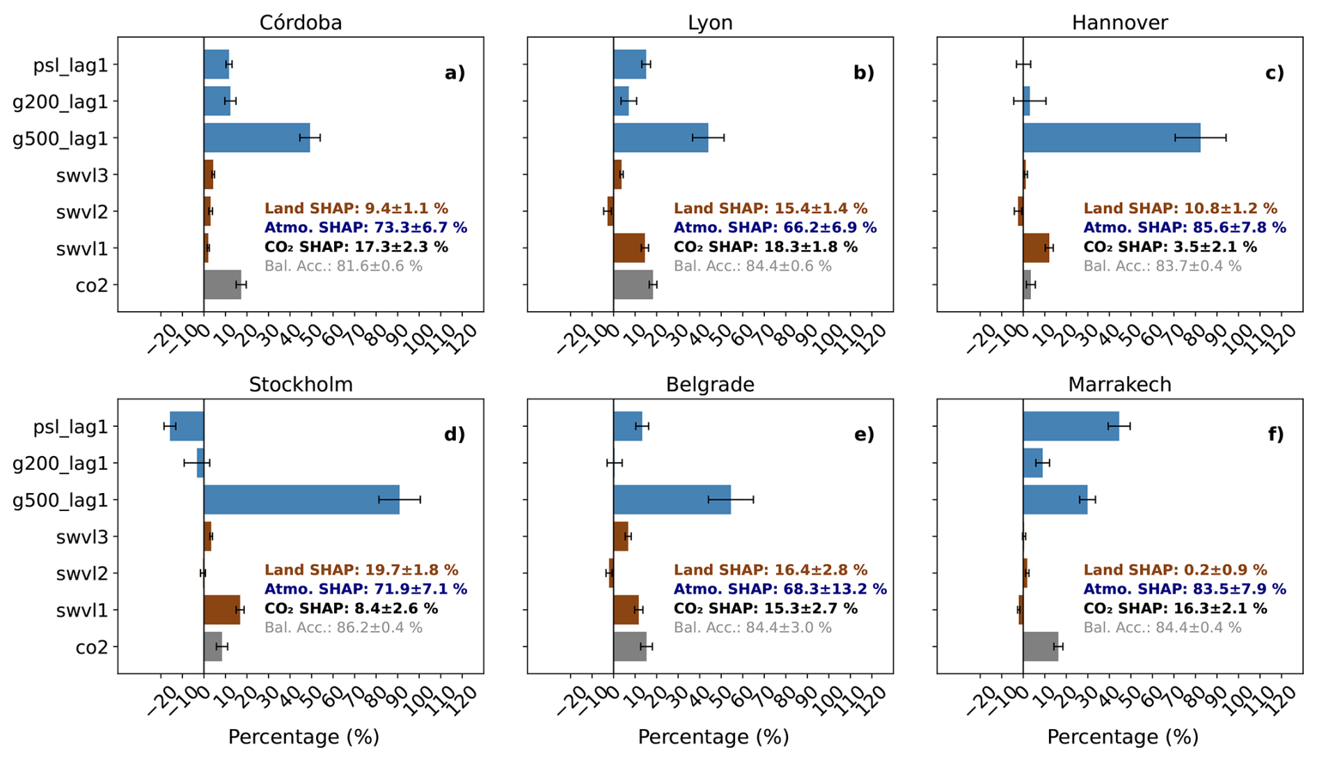
Figure 5 Extreme class prediction mean SHAP value percentage for all locations using the CombinedModel taking the 50 % most confident predictions. The x-axis represents the percentage contribution of each feature relative to the total sum of mean absolute SHAP values. Error bars indicate the Standard Error of the Mean (SEM) derived from the 20-member ensemble, representing the uncertainty across different model initializations. The colored text box provides the aggregated percentage contributions for Land and Atmospheric components, as well as the CO₂ contribution, with associated ensemble uncertainties (±SEM). The balanced accuracy of the model is also indicated.

The atmospheric circulation has the largest importance (66 %–86 %) at all locations. Apart from being intuitive, this result is in line with for instance Uckan et al. (2025), who show that geopotential height at 500 hPa is the dominant driver of hot extremes worldwide, particularly in mid-latitudes, and that the relevance of atmospheric drivers increases with the duration of the hot event. The Land SHAP value is more important in northern regions. In Marrakech, the land SHAP percentage is very small (0.2 %), which is reasonable given the region is generally very dry during the summer, therefore the interannual variability of soil moisture is low and consequently coupling with atmosphere very little. Córdoba shows a higher percentage (9.4 %) explained by the land SHAP compared to Marrakech. The importance of swvl3 in Córdoba is slightly larger than swv1 and swvl2, consistent with top soil layers being fully dissicated in summer. The land SHAP value increases for higher-latitude locations, being specially important in Lyon. This result is in line with Jach et al. (2022), who assessed how changes in the mean temperature and moisture influence the land–atmosphere coupling strength over Europe.

As for the large-scale fields, there is a predominance of the geopotential at 500 hPa, with only Marrakech having sea level pressure being more important than the atmospheric fields at higher altitude.

The atmospheric CO₂ feature has a higher importance in regions that exhibit a stronger trend in extreme temperature days (see Fig. 4). Except for Hannover, the importance of the CO₂ feature is generally high (> 10 %). These differences among locations align with the work of Sippel et al. (2020) in that different regions show different responses to climate change, with the forced fingerprint manifesting through varying signal-to-noise ratios across the globe.

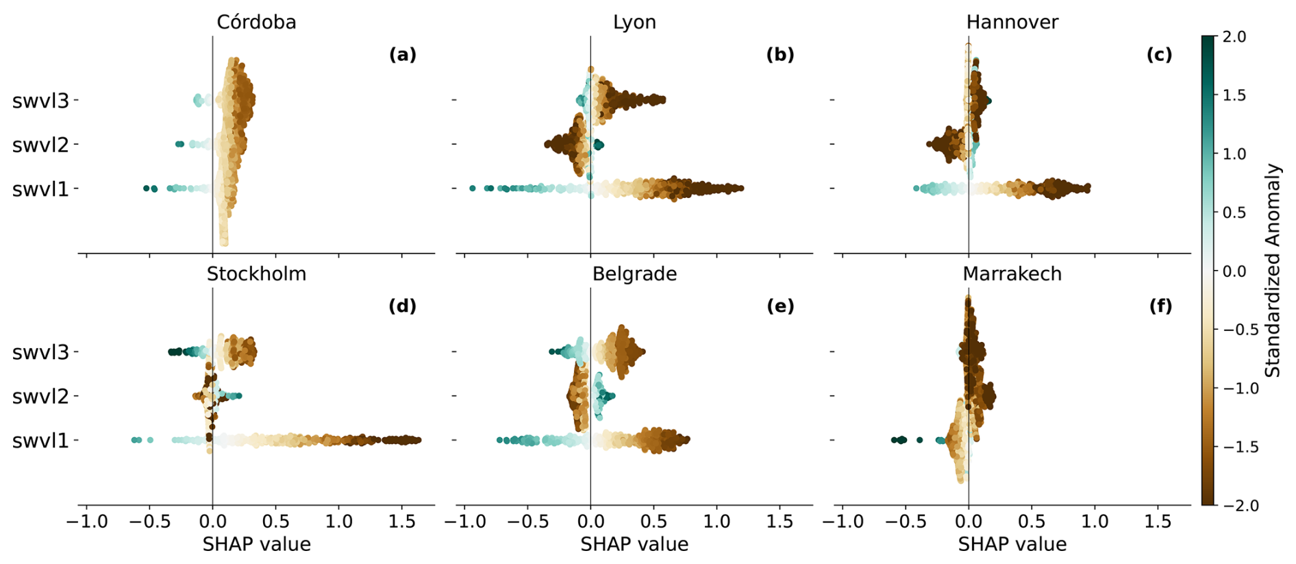
Figure 6 SHAP values swvl[1,2,3] across samples test phase for the 50 % most confident predictions and extreme class. The x-axis represents the SHAP value of the sample and the y-axis the soil moisture level feature used in the model. The colour bar shows the value of the standardized anomalies of the soil moisture level.

Lastly, Fig. 6 illustrates how SHAP values vary with standardized anomalies of the soil-moisture predictors. For the upper soil layer (swvl1), negative anomalies are generally associated with positive SHAP contributions to the extreme class, consistent with the expected amplifying role of surface drying on hot extremes. In contrast, the relationship for the intermediate layer (swvl2) is less robust across locations, with weak mean contributions and substantial uncertainty. This behaviour likely reflects the strong correlation between neighbouring soil layers, which limits the model's ability to uniquely attribute predictive skill to swvl2 independently of swvl1. The deepest layer (swvl3) shows a more location-dependent behaviour, with a clearer contribution in Córdoba. The inverse SHAP–anomaly relationship identified for the dominant shallow soil-moisture contribution is also found in the 80th percentile model (not shown) and the model using SPEI (see Fig. D3), further confirming the robustness of the land-drying feedback mechanism identified by the model across different methodological choices.

The discussed explainability results are robust to the definition of an extreme event. For the 80th percentile model, the SHAP values (see Fig. D2) show the same main characteristics: the circulation component remains dominant (63.9 %–83.7 %), and the land component still exhibits a northward gradient in importance, though less pronounced. Except for Córdoba and Marrakech, the relative contribution of soil moisture is, however, generally smaller than for the 90th percentile model. This would suggest a more marginal role of soil moisture in less severe heat events for which the land–atmosphere feedbacks, a key amplifier of extreme temperatures, may not be fully activated. The fact that the land component contribution is similar for Marrakech and Córdoba in the two extreme definitions might be an indication of the land–atmosphere coupling being rarely activated there in summer due to the scarce coupling in very dry conditions, independently of the extreme definition. Land variables could play an even more important roles for more restrictive percentiles like the 95th percentile. However, as mentioned in Sect. 3.1, we do not show the explainability results for this case due to the lack of stability in the accuracy metrics when using this higher percentile as threshold to identify extremes.

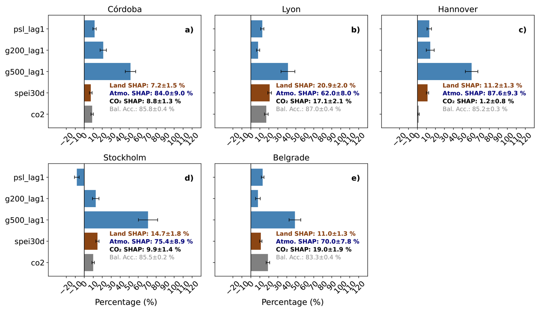
Figure 7 Same plot as in Fig. 5 but for the model using E-OBS observational data and the SPEI30d index as a proxy for the soil moisture feature. The 90th percentile is still used for the extreme event definition.

To further constrain our analysis with observational records and evaluate the framework's performance beyond reanalysis data, we examine the SHAP results using observational data from E-OBS for TX and the SPEI30d drought index as a proxy for soil moisture (Fig. 7).

The driver contributions are overall consistent when using observational data from E-OBS instead of ERA5-Land for TX and the SPEI drought index as a proxy for the soil moisture variables. In general, the XAI results reproduce the established north–south gradient in land driver importance and the dominant importance of the atmospheric circulation component (see Fig. 7). In Fig. D3 we see that we also have a negative correlation between SHAP value and SPEI30d feature values.

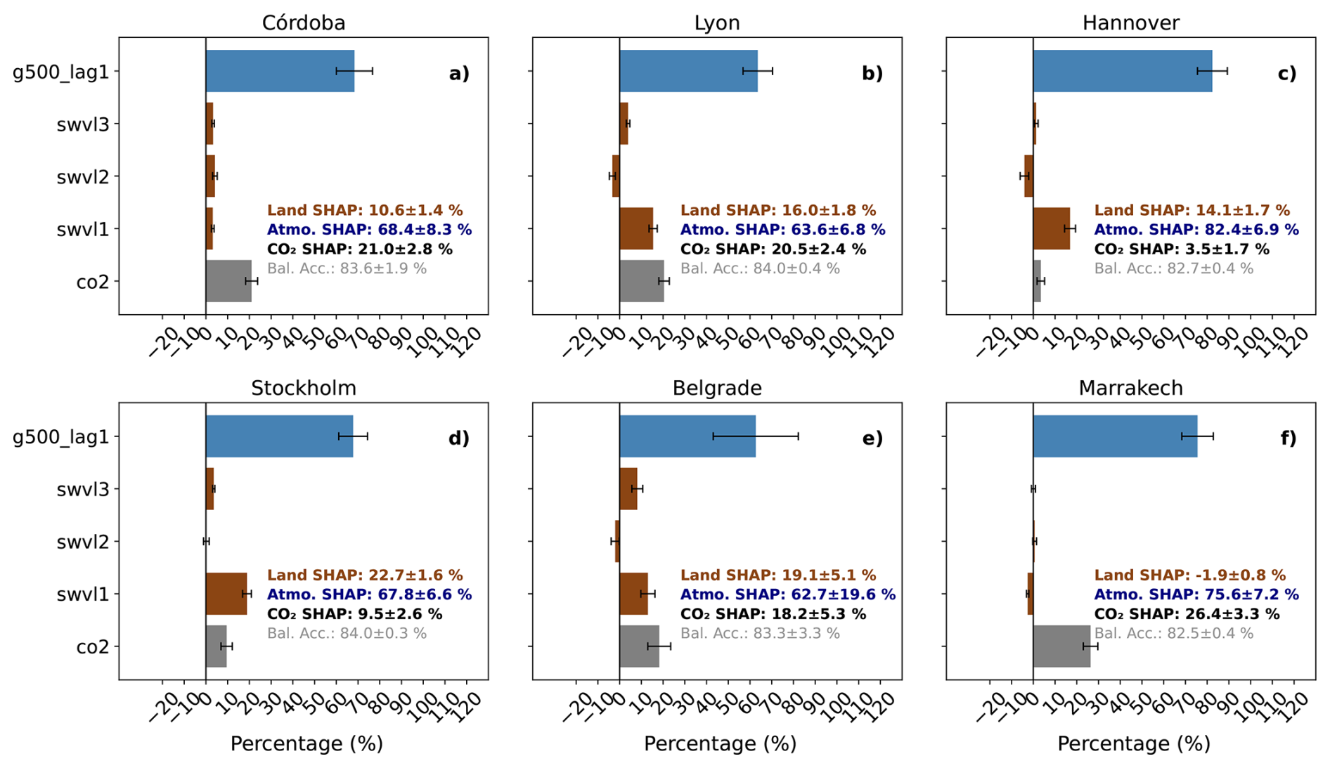
When using the SPI index, the XAI results for the land component are less similar to the original ERA5-Land soil moisture results (see Fig. D4). Although a correlation analysis between the indices and soil moisture shows that SPEI generally correlated slightly better with soil moisture than SPI (see Fig. C1), the differences are relatively small. Nevertheless, the XAI outcomes reveal that SPI captures less of the original soil moisture signal. This aligns with physical understanding, as SPEI, by incorporating evapotranspiration, provides a more comprehensive representation of surface moisture balance and its coupling with the atmosphere than SPI, which is based solely on precipitation. This suggests that for the future application of this framework to climate models, SPEI is a suitable proxy that avoids inter-model differences in representation of soil layers, and therefore allows more consistent evaluation of the relationships across different models and observations/reanalysis.

is a suitable proxy that avoids inter-model differences in representation of soil layers in therefore allows more consistent evaluation of the relationships across different models and observations/reanalysis

Overall, the feature with the largest importance shown by the XAI results for the g500 field. As a result, we decided to test the robustness of the model when using only this field to represent the atmospheric circulation features, obtaining similar results to the ones discussed above (see Fig. D5). The predominance of the g500 field is not surprising, as it is known to have a key role in determining the state and evolution of the troposphere, as well as a key indicator of the climate change response (Christidis and Stott, 2015). Lemus-Canovas et al. (2024) and Quesada et al. (2012) also show the important role of the atmospheric circulation component in triggering the heatwave event, and the land compound acting as an amplifier of extreme conditions. Moreover, Wilcke et al. (2020) highlight the importance of circulation in the 2018 summer heatwave over Stockholm, and its capability to force warm, long-lasting conditions without much contribution of surface feedbacks.

3.3 Case study: Summer heatwave Córdoba 2021

For the first case study, we test the CombinedModel during the period 10 to 20 August 2021 in the Córdoba region, when a record-shattering heatwave struck the Iberian Peninsula. During this period, temperatures up to 47.6 °C were registered in La Rambla (Córdoba) (AEMET, 2021).

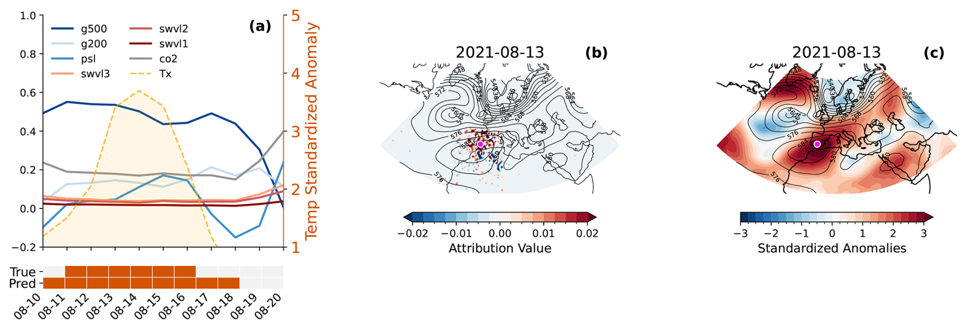
Figure 8 SHAP values for extreme class predictions for the Córdoba case study. (a) SHAP values temporal evolution for the circulation features and the three soil moisture levels. We additionally include temperature standardized anomalies (shaded orange area). The true and predicted labels are shown at the bottom, with orange indicating and extreme (class 1) and gray indicating a non-extreme day (class 0). (b) SHAP spatial distribution for the peak-day of temperature anomaly (14 August). SHAP values with absolute magnitude smaller than 0.008 are masked to improve visual clarity. g500 contours for the day prior to the peak are included. (c) Standardized anomalies of geopotential at 500 hPa in colour and data in contours for the geopotential at 500 hPa for the day prior to the temperature anomaly peak (13 August). The magenta dot in panels (b) and (c) marks the location of Córdoba.

Figure 8a shows the temporal evolution of the extreme class SHAP values for the atmospheric circulation features in terms of mean absolute SHAP (spatially aggregated), and the three soil moisture levels. Additionally, it shows the standardized temperature anomalies and the true and predicted labels. By looking at the predicted labels, we can see that the model correctly predicts all the true positives of this event but yields false positives at the developing and decaying stages of the heatwave event. Figure 8b shows the SHAP values for the g500 feature at the temperature anomaly peak identified in Fig. 8a (14 August 2026). Grid points with |SHAP| < 0.008 are masked out for clarity. Lastly, Fig. 8c displays the standardized anomalies for the lag1 (13 August 2021) of the g500 field (colours) and the geopotential height at 500 hPa data (black contours). During the thirteenth of August, the positive anomalies and anticyclonic pattern are right above the Iberian Peninsula, and our model gives mainly positive SHAP values for that region, showing strong locality around the predicted location. This signal starts to be strong and positive when the positive anomalies reach the predicted location (Fig. 8a).

The soil moisture anomalies during this event are negative but not especially low (not shown), resulting in SHAP values for the soil moisture levels being small and remaining quite constant. A curious result is the CO₂ being generally the second most important feature. This suggests that even for a specific extreme event like this one, we can identify a clear anthropogenic contribution.

3.4 Case study: Summer heatwave Hannover 2018

We select the Hannover region for the second case study to represent a different land–atmosphere coupling regime, characterized by higher soil water content, compared to the Córdoba region (Seneviratne et al., 2006). We focus on the 2018 European heatwave, which was an exceptional climatic event that brought prolonged periods of extreme heat and drought to much of Northern and Central Europe, including Germany.

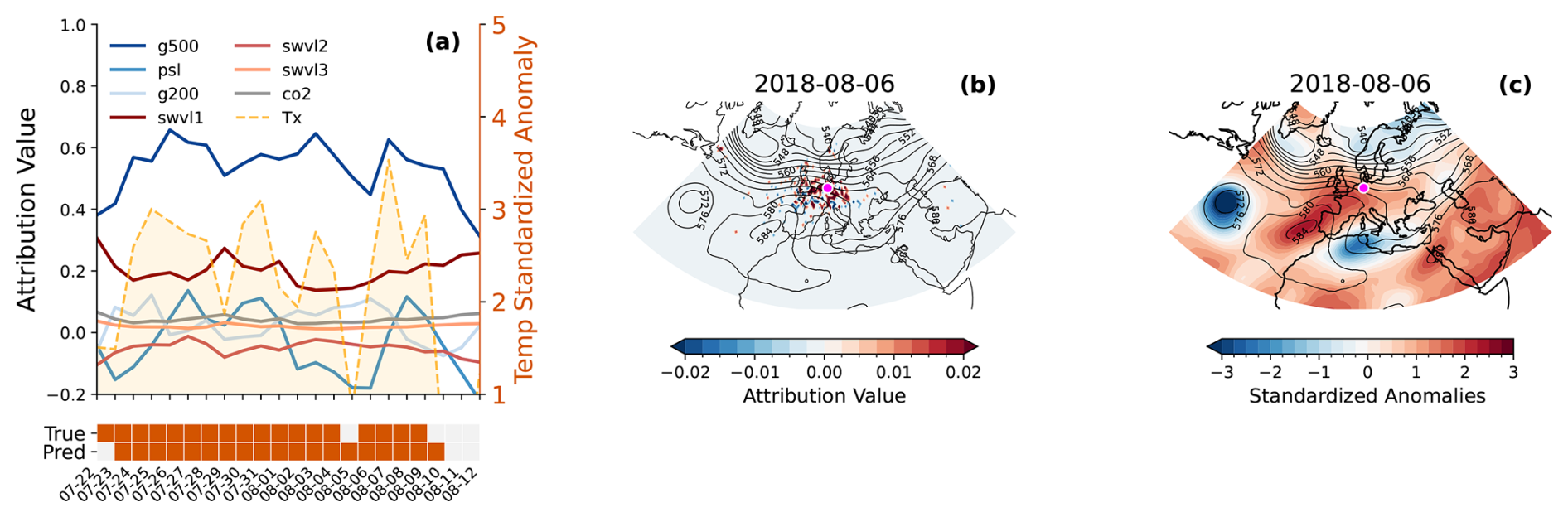
Figure 9 SHAP values for extreme class predictions for the Hannover case study. (a) SHAP values temporal evolution for the circulation features and the three soil moisture levels. We additionally include temperature standardized anomalies (shaded orange area). The true and predicted labels are shown at the bottom, with orange indicating and extreme (class 1) and gray indicating a non-extreme day (class 0). (b) SHAP spatial distribution for the peak-day of temperature anomaly (7 August). SHAP values with absolute magnitude smaller than 0.008 are masked to improve visual clarity. g500 contours for the day prior to the peak are included. (c) Standardized anomalies of geopotential at 500 hPa in colour and data in contours for the geopotential at 500 hPa for the day prior to the temperature anomaly peak (6 August). The magenta dot in panel (b) marks the location of Hannover.

The period selected is 22 July 2018 to 12 August 2018. In Fig. 9 we show the same type of plots as in the former case study, with the same filtering for the SHAP values applied in Fig. 9b. Again we see a strong locality in the spatial SHAP values for g500, with positive values surrounding the predicted location, where the positive anomalies are located. The spatial distributions are noisy for the rest of circulation variables, but they all explain less than 10 % of the total mean absolute SHAP value. In Fig. 9a we can see that in this case the level one of soil moisture plays a more important role compared to the Córdoba event. The soil moisture at level one has positive SHAP values during the whole period, which is comparable to g500 in magnitude for some of the days. Regarding the CO₂ concentrations, in this case its relevance is much lower compared to the Córdoba case.

4 Conclusions

In this study, we quantify the contribution of soil moisture, atmospheric circulation and CO₂ forcing to extreme temperature events during the boreal summer using an explainable ML approach. We focus on six locations with different evaporative regimes. Based on a percentile definition of extremes, we find an increasing trend in the yearly count of extreme days during summer for Córdoba, Lyon, Belgrade, and Marrakech regions.

To ensure the robustness of the model predictions, we train an ensemble of 20 members and analyse the 50 % most confident predictions across all observed cases. Balanced accuracy increases consistently with the percentage of confidence using the CombinedModel, indicating stable predictive skill. The area under the ROC curve also improves with confidence. We further tested this robustness by applying our framework to different extreme definitions and data sources. The model trained on the 80th percentile definition showed equally robust predictive performance, while the model trained on the more stringent 95th percentile definition exhibited less stable behaviour due to the high class imbalance, leading us to disregard its explainability outputs. Furthermore, the framework demonstrated reliable performance when using observational data for TX and for computing SPI/SPEI drought indices as proxys for soil moisture, with SPEI giving qualitatively more similar results to the model using ERA5 data for the atmospheric circulation and the soil moisture levels.

To help interpret the model prediction, we use SHAP values, which allows us to assess the marginal contributions of the atmospheric circulation, land and atmopspheric CO₂ features. The reader must keep in mind that the explainability results represent the interpretations done by the model, and we cannot assume that these results represent the reality. We are ensuring a treatment of part of the existing epistemic uncertainty when using this model, but different architectures or different models might differ in the results. The explainability results show that circulation features, especially the geopotential at 500 hPa, dominate the prediction of extreme events across all locations (66.2 %–85.6 %). The land component shows a regional differing behaviour: its importance increases in temperate and northern regions (10.8 %–19.7 %), while remaining negligible or moderate in a dry/transitional location like Córdoba and a dry one like Marrakech (Hsu and Dirmeyer, 2023), representing 9.4 % and 0.2 % of the total SHAP respectively.

The dominant soil-moisture contributions – particularly from the uper layer – show an inverse relationship between moisture anomalies and SHAP values, consistent with the well-documented role of dry conditions in enhancing the probability of extreme heat events (Hirschi et al., 2011; Seneviratne et al., 2006). Attribution for the intermediate layer is weaker and less robust, likely because strong inter-layer correlations make its independent contribution difficult to isolate. The land component importance increases from the 80th to the 90th percentile extreme definition. This suggests that land variables could play an even more important role for more extreme events (e.g. using a 95th percentile extreme definition). This could not be analysed with the presented methodology due to class imbalance. CO₂ SHAP contributions are substantial in locations where we detect a trend in the yearly extreme count, suggesting that the model captures the long-term forcing signal.

Furthermore, the core patterns of driver contributions identified by the model are robust to a different definition of the extreme events and to the use of observational data from E-OBS instead of ERA5-Land. The north–south gradient in land driver importance and the dominance of atmospheric circulation are consistently reproduced in the analysis using the 80th percentile extreme definition, albeit with a reduced relative contribution from soil moisture, likely due to the inclusion of less severe events. Moreover, the regionality of the land component is robustly recovered when using observational temperature data and the SPEI drought index as a proxy for soil moisture. The SPI index, which lacks the evapotranspiration component of SPEI, resulted in a weaker land signal, underscoring the importance of representing more accurately surface water balance for capturing land–atmosphere feedbacks and confirming that SPEI provides a more physically comprehensive proxy for this purpose.

We also analyse two case studies to provide further insights on the networks predictive behaviour. For the 2021 Córdoba heatwave, the model attributes the dominant contribution to the atmospheric circulation, with a mainly positive SHAP signal over the Iberian Peninsula when positive 500 hPa geopotential are placed in the region. We identify a clear anthropogenic contribution due to the high CO₂ SHAP value in this event. The land variables play a minor role in this case, with anomalies close to zero for the three soil moisture levels. During the 2018 Hannover heatwave, we see an enhanced importance of the land component, especially the first soil moisture level, with positive SHAP values comparable to the g500 circulation feature during the first days of the event. Again, we see a strong locality in the spatial distribution of SHAP values. In this second case study, CO₂ plays a minor role.

These results are consistent with findings about the central role of atmospheric circulation in driving extreme temperature events and highlight the regionally dependent modulation by soil moisture (Fischer et al., 2007; Barriopedro et al., 2023; Quesada et al., 2012). The explainability technique used allows us to attribute data-driven predictions to physical drivers, offering a diagnostic framework that can assess the contribution of individual components to extreme events. We have demonstrated that this framework and its conclusions are robust to the choice of extreme event threshold (if the class imbalance is not too strong) and to the use of observational data instead of reanalysis data.

Our findings on the role of atmospheric circulation in driving daily temperature extremes support the findings of Uckan et al. (2025), who showed that the geopotential field is the most relevant feature over 59.9 % of global land at a 1 d scale and 67.9 % at a 7 d scale. We confirm the importance of the atmospheric circulation using a different ML architecture, adding robustness to this result. Additionally, using a ConvNeXt model for atmospheric fields allows us to identify the spatial regions to which the model attributes higher importance, further demonstrating the ability of XAI to reveal spatial patterns in weather and climate problems, as shown by Davenport and Diffenbaugh (2021) and Mayer and Barnes (2021) using LRP. While recent studies have increasingly employed XAI to identify regional climate drivers and sources of predictability (e.g., Zhang et al., 2024; Van Straaten et al., 2023; Mamalakis et al., 2023b), our work specifically leverages XAI to disentangle the relative roles of atmospheric circulation and land-surface conditions in driving localized hot temperature extreme events.

The role of soil moisture in modulating the occurrence of extremes has been highlighted by Materia et al. (2022) and Seneviratne et al. (2006), showing that dry soils intensify and prolong heat extremes, while wet soils suppress heatwaves. Here, we support these findings on the modulating effect of the land–atmosphere coupling by analysing the correlation between soil moisture anomalies and corresponding SHAP values. Our work contributes to disentangling the components of this coupling and quantifying their roles using XAI. We further quantify the influence of soil moisture at three different depth levels and find that, on weather time scales, the level closest to the surface plays the largest role for humid/transitional regions, whereas the bottom layer is more important for a dry/transitional location like Córdoba.

Finally, we include a quantification of the role of atmospheric CO₂. Including this feature allows us to account for the trend in the occurrence of hot extremes due to global warming, without encountering the complications of detrending the data when splitting it into training, validation, and testing sets in ML studies.

Future work should include testing the robustness of the results across different model architectures. Analysing additional locations in future work may help gain insights into the regional variability of the results. Including variables like humidity fluxes or information on aerosol composition in each location could also provide complementary information on the physical processes modulating temperature extremes during boreal summer. The presented XAI methodology could also be applied to evaluate the importance of the different drivers in CMIP6 dynamical models or in Subseasonal to Seasonal to Decadal Prediction Systems.

Overall, this study provides a physically interpretable, data-driven framework to disentangle the contributions of atmospheric circulation, land surface conditions, and anthropogenic forcing to summer temperature extremes. By combining a robust machine learning method with an ML explainability technique,we provide a framework that can support model development and climate attribution efforts. Our results underscore the dominant influence of atmospheric circulation and the modulating role of soil moisture, revealing consistent regional signals across different locations. These findings highlight the potential of explainable machine learning as a complementary tool for climate diagnostics and pave the way for more comprehensive, process-based assessments of future temperature extremes.

Appendix A

A1 LOESS smoothing

To improve the robustness of daily climatology percentiles estimates, we use a local polynomial regression (LOESS) as proposed in Mahlstein et al. (2015). This method smooths the raw climatology by fitting a regression locally at each point using a subset of neighbouring days weighted by distance. The weights w_i applied to each point in the local window are based on their normalized distance d_i to the estimation point, using the tricubic function:

$$w_i=\left\{\begin{array}{ll}{\left(\mathrm{1}-|d_i{|}^{\mathrm{3}}\right)}^{\mathrm{3}},& \text{if }\left|d_i\right|\le \mathrm{1}\\ \mathrm{0},& \text{if }\left|d_i\right|>\mathrm{1}\end{array}\right.$$

where $d_i=\frac{x_i-x}{h}$ is the distance between the input point x_i and the target point x, scaled by the distance h to the farthest neighbour in the local window. This ensures that the weights smoothly decay to zero at the edges of the window and are strictly zero beyond it.

In practice, this means we apply LOESS to the raw daily climatology or percentile values to obtain a smoother and more stable annual profile. This is particularly important when dealing with small sample sizes or high daily variability, where simple averaging can lead to noisy or misleading estimates. This smoothing step ensures that the resulting threshold and climatology estimates are not overly influenced by isolated values or short-term fluctuations, which is especially relevant for extreme event detection on a daily basis.

A2 Cross-entropy loss function

The Cross Entropy Loss function is defined as:

$$\begin{array}{}\text{(A1)}& \mathcal{L}={\displaystyle \frac{-\mathrm{1}}{N}}\sum _i{y}_i\cdot \log \left(p_i\right)+(\mathrm{1}-y_i)\cdot \log (\mathrm{1}-p_i)\end{array}$$

where p_i is the probability of class 1, (1−p_i) the probability of class 0, and y_i is the true label. This loss function is widely used in binary classification tasks in ML.

Appendix B: Statistical and robustness results

Table B1 Summary of extreme event counts by site and period for different extreme definitions. Yearly extreme count sum is shown for the different locations, for the training (80 % of 1950–2013), validation (20 % of 1950–2013) and test (2014–2024) periods. E corresponds to the extreme class and NE to the non-extreme class. Additionally, we show the randomly selected years for the training and validation sets.

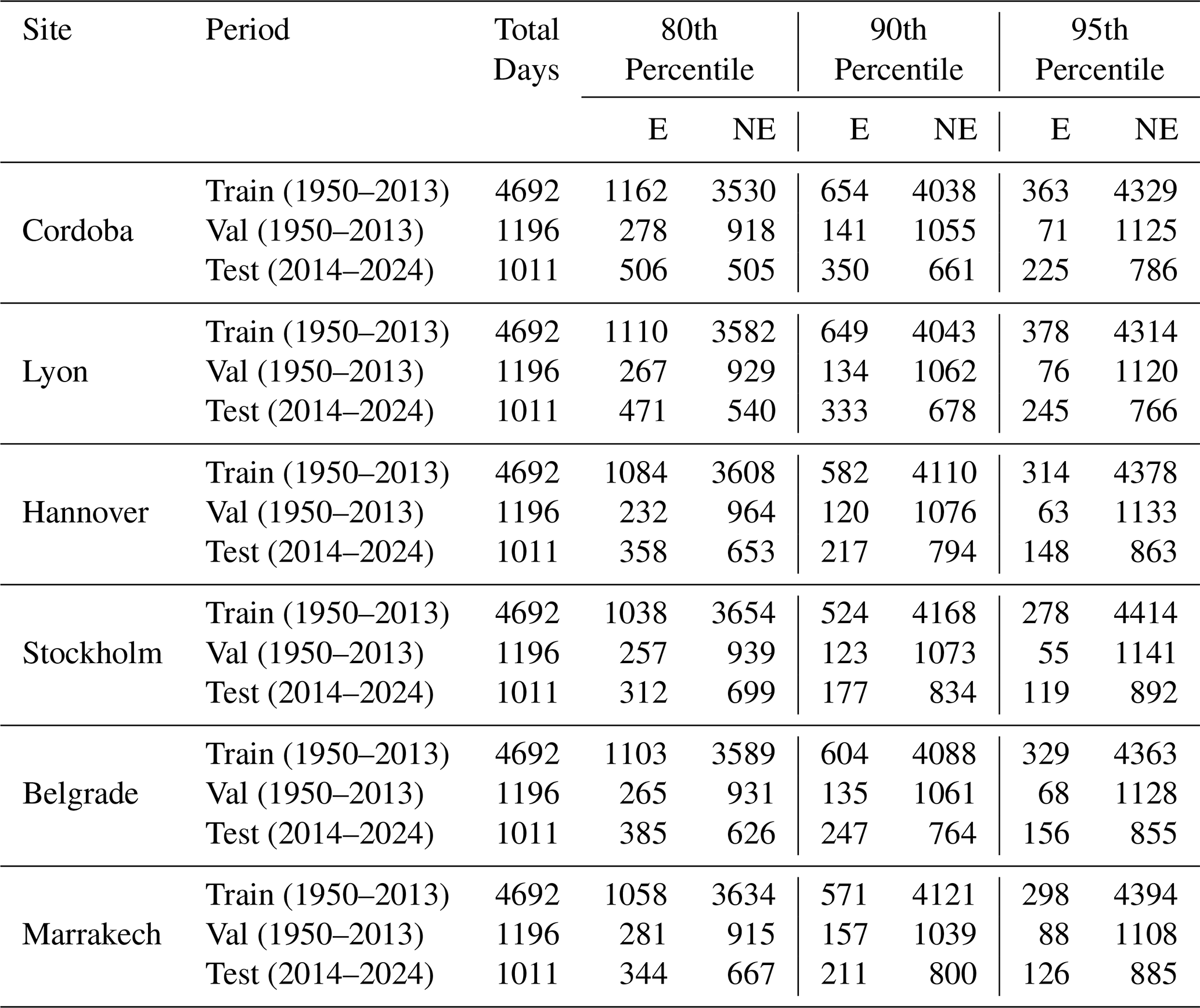
Training years: 1951, 1953, 1954, 1958–1986, 1988–1991, 1993, 1995–1998, 2000, 2002–2005, 2007, 2009, 2011–2013.
Validation years: 1950, 1952, 1955, 1956, 1957, 1987, 1992, 1994, 1999, 2001, 2006, 2008, 2010.

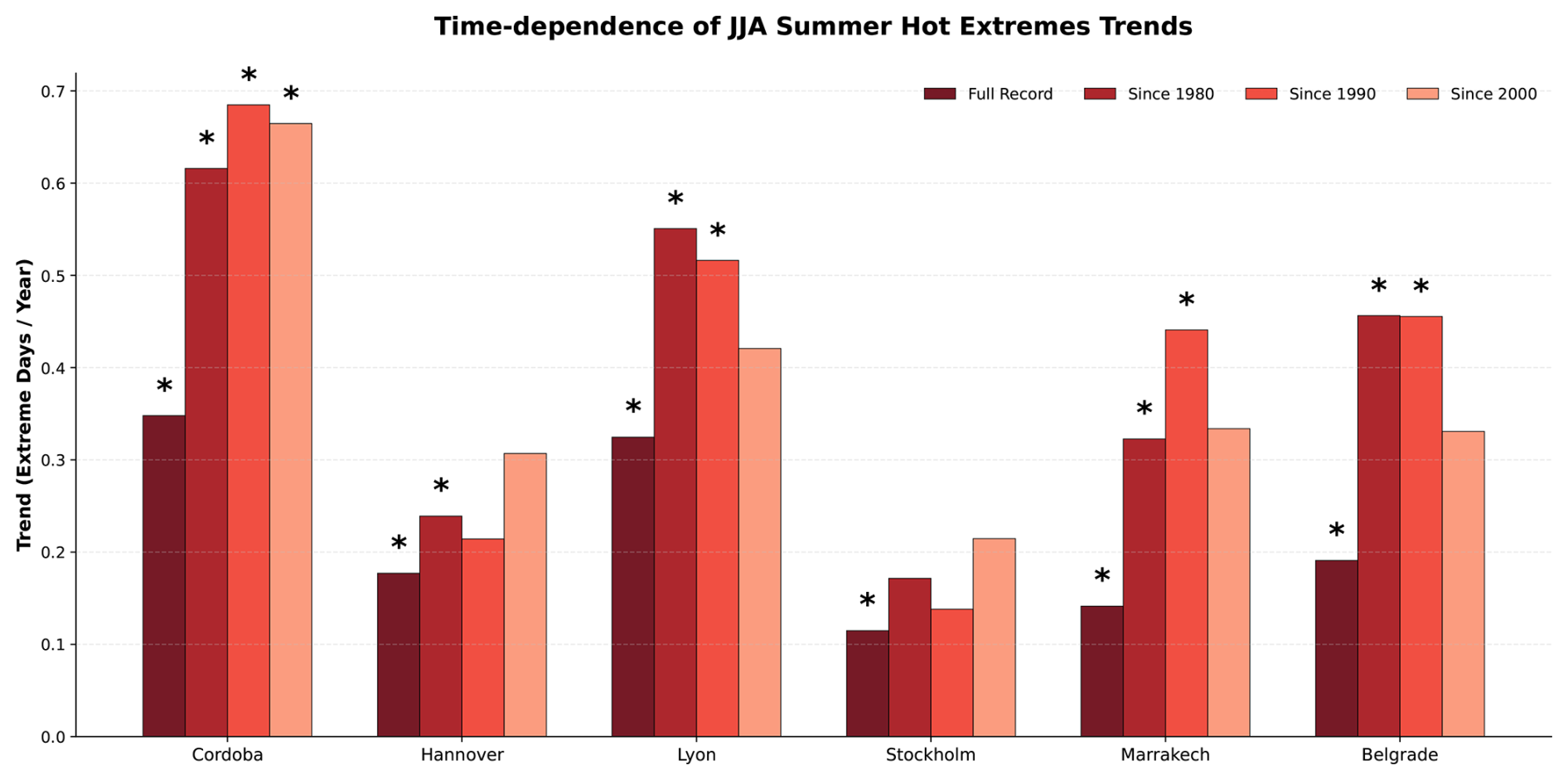
Figure B1 Trends in JJA Summer Hot Extremes across different time periods. Bars represent the slope coefficient (trend magnitude) of a linear regression applied to the yearly count of extreme days for four periods: the full available record (dark red), since 1980 (red), since 1990 (light red), and since 2000 (lightest red). Asterisks (^∗) indicate trends that are statistically significant at the 95 % confidence level, determined using a t-test on the slope coefficient.

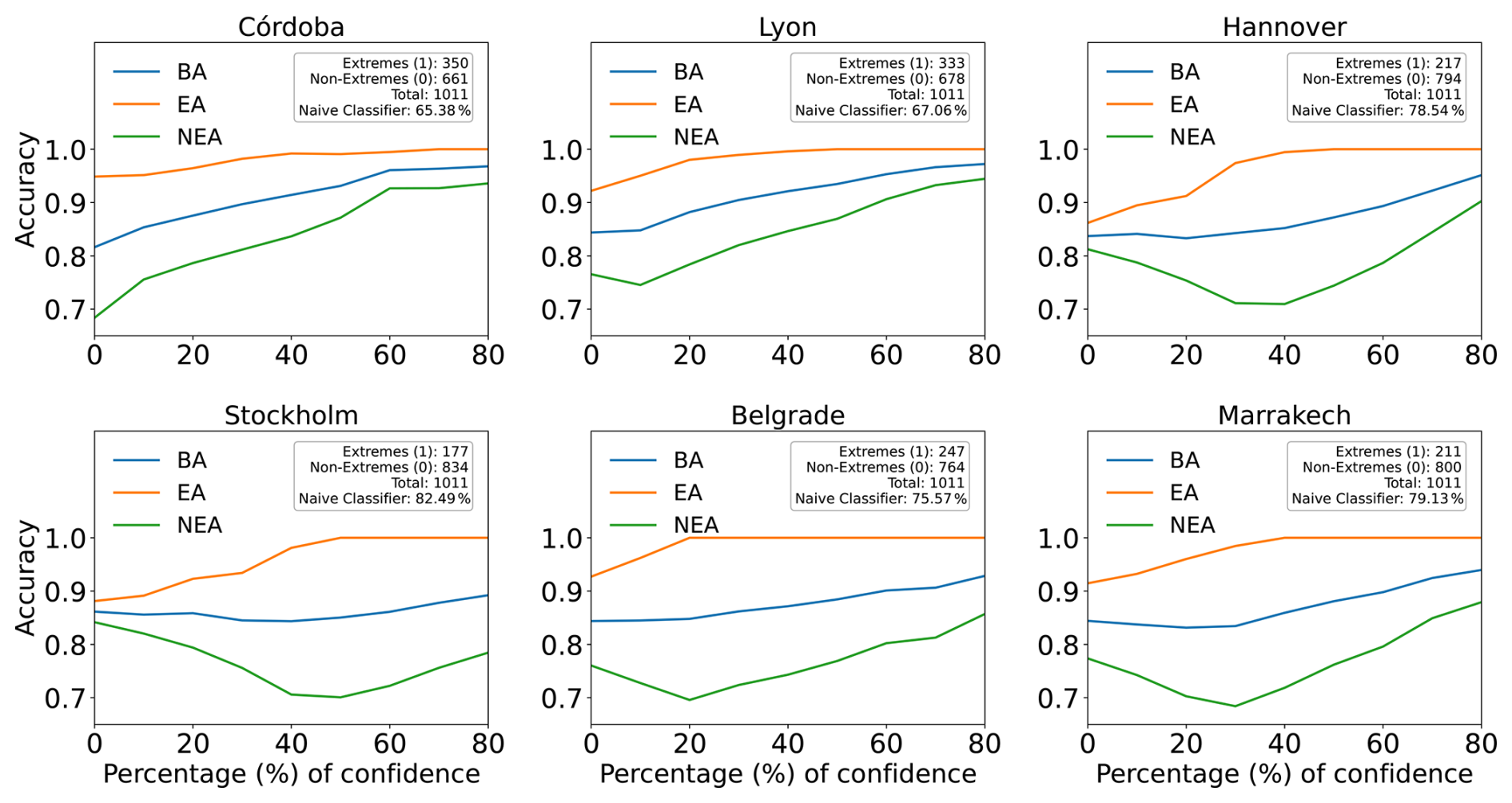
Figure B2 Change in accuracies for the Combined Model for different percentages of confidence using the 90th percentile extreme definition. In the x-axis the percentage of confidence taken, and in the y-axis the accuracies. EA, NEA and BA in the legend stand for extreme accuracy, non-extreme accuracy and balanced accuracy respectively. The text box shows the sample size and the random chance of the naive classifier.

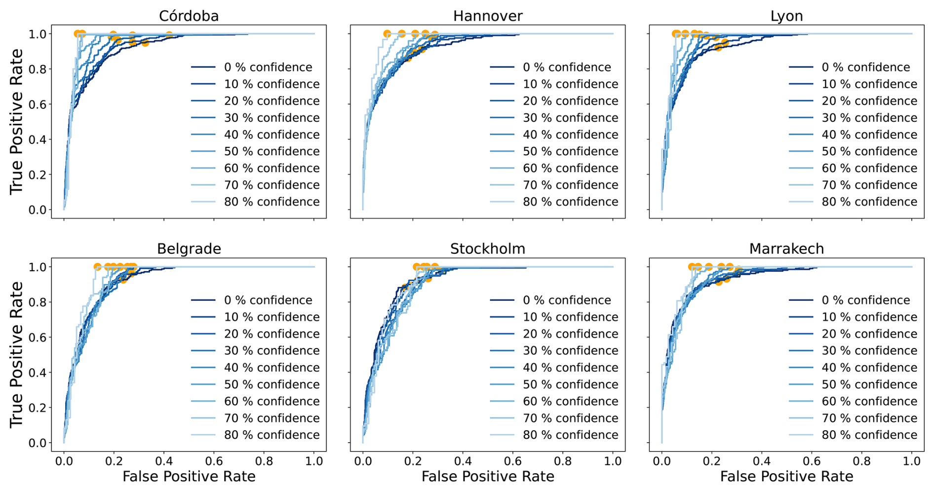
Figure B3 Change in ROC curves for the Combined Model for different percentages of confidence using the 90th percentile extreme definition. In the x-axis the false positive rate and in the y-axis the true positive rate. The legend shows the different percentages of confidence taken.

Figure B4 Same plot as in Fig. B2 but for the 80th percentile definition of extreme.

Figure B5 Same plot as in Fig. B2 but for the 95th percentile definition of extreme.

Appendix C: Drought indices correlations

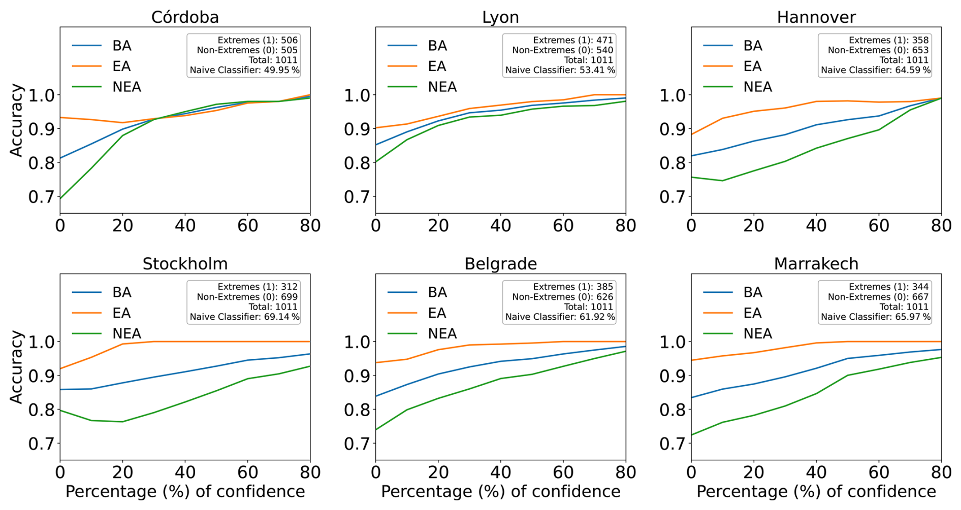
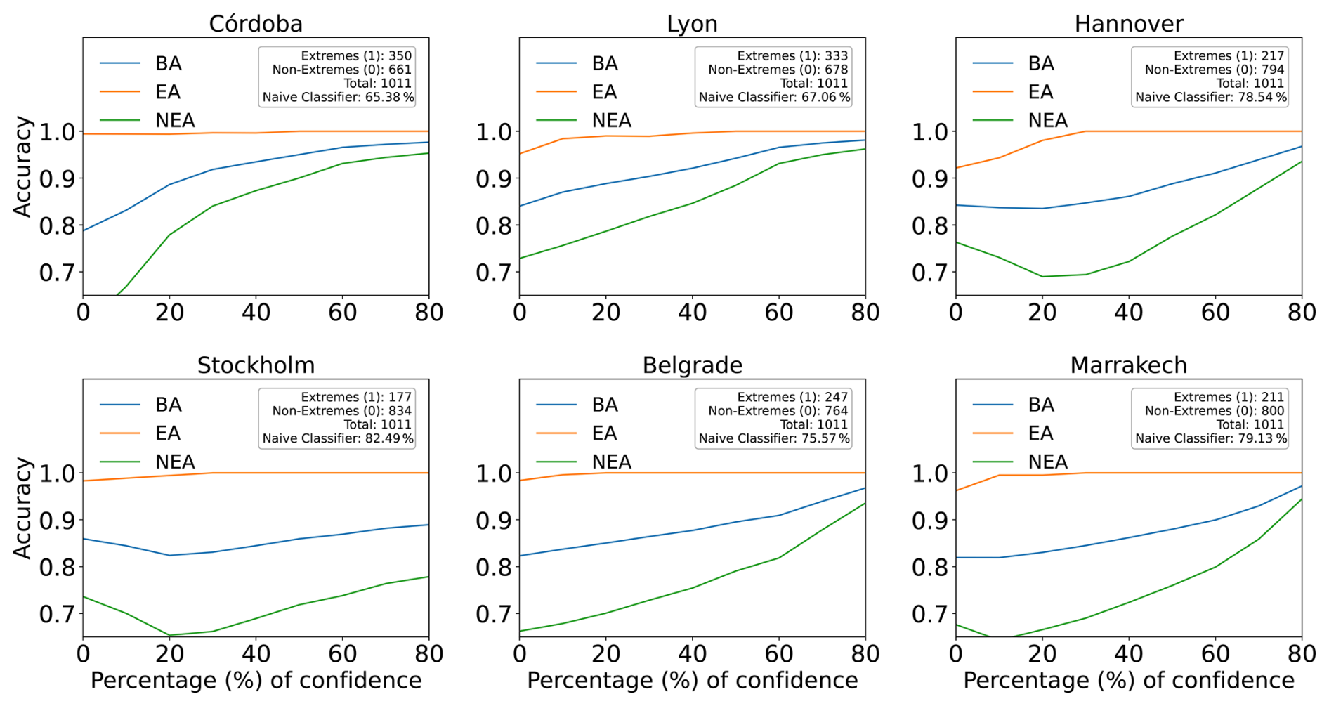
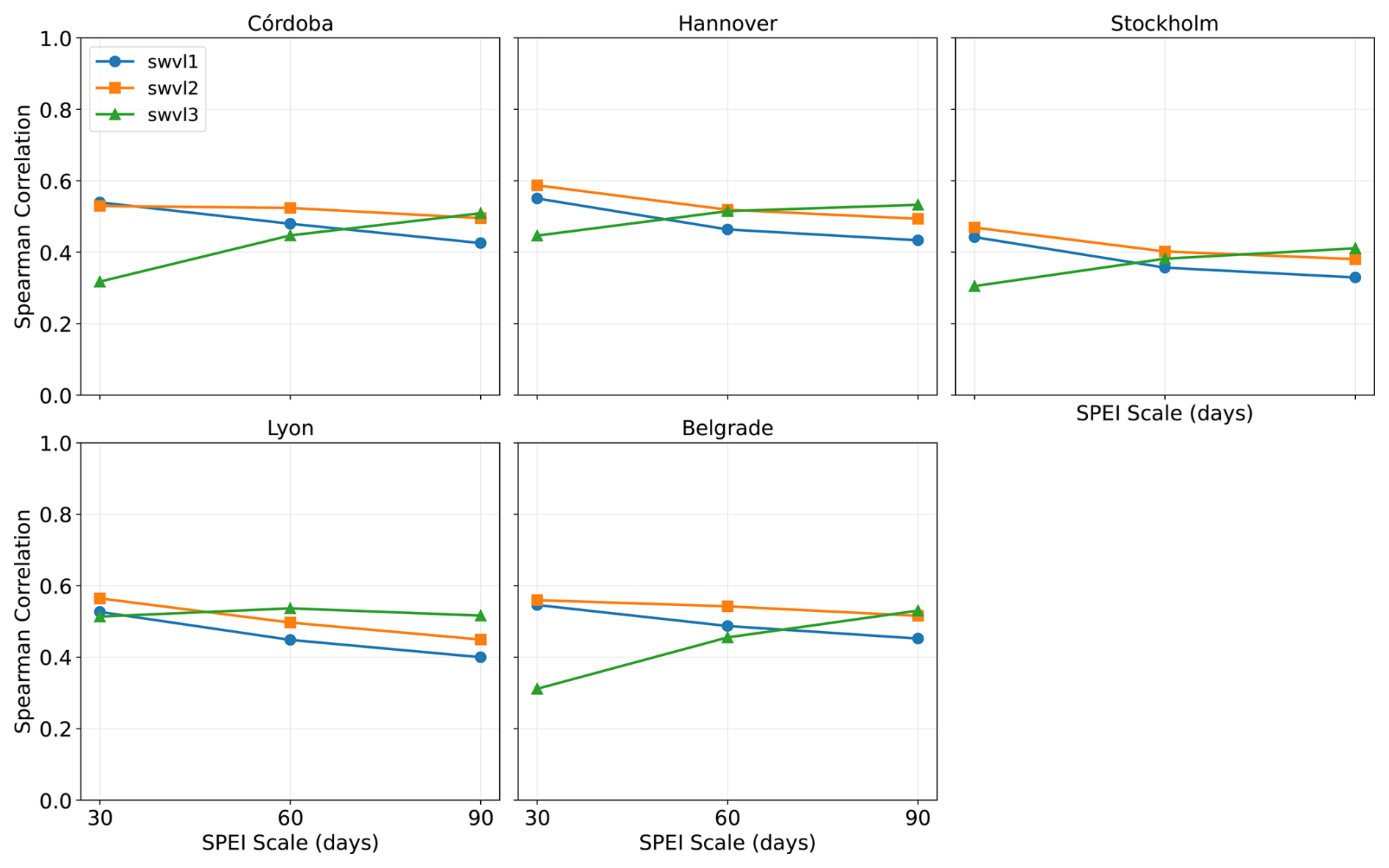
Figure C1 Spearman correlation between the three soil moisture levels (swvl1, swvl2, swvl3) and the SPEI index computed at three different time scale using the E-OBS gridded data. In the x-axis the scale used to compute the SPEI index and in the y-axis the resulting spearman correlation. The legend indicates the three original soi moisture levels used in the DL model.

Figure C2 Same plot as Fig. C1 but using the SPI drought index instead.

Appendix D: XAI results

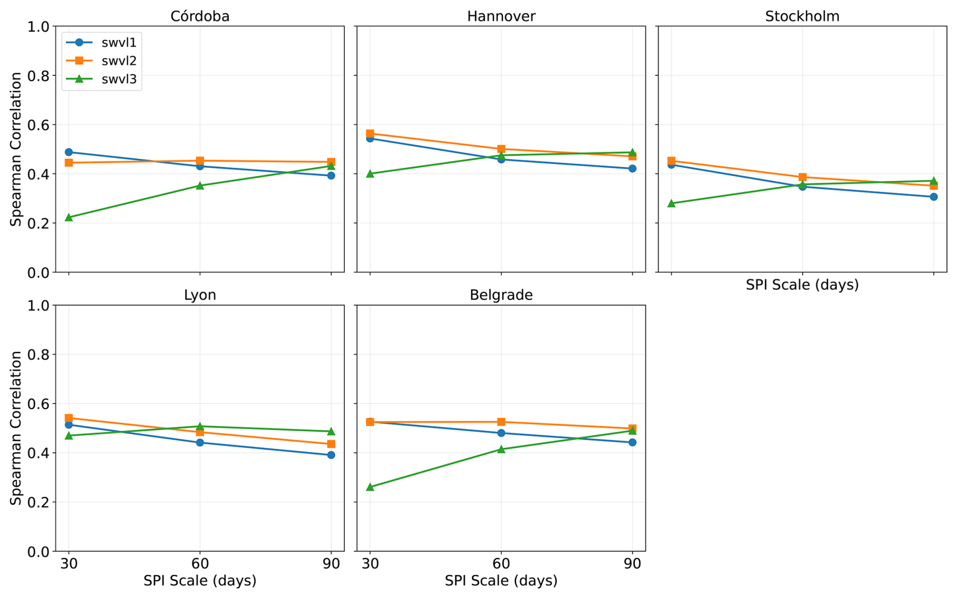
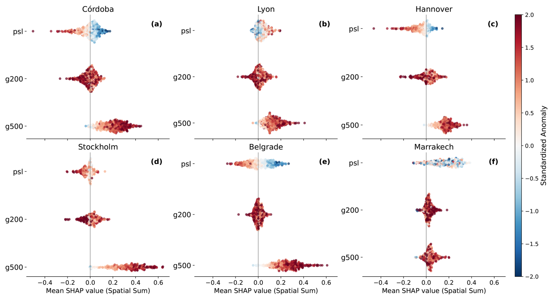
Figure D1 Same plot as in Fig. 6 but for the atmospheric circulation features. We sum up the SHAP values and averaged the standardized anomalies of the circulation variables in a 400 km by 400 km region surrounding the target location.

Figure D2 Same plot as in Fig. 5 but for the 80th percentile definition of extreme.

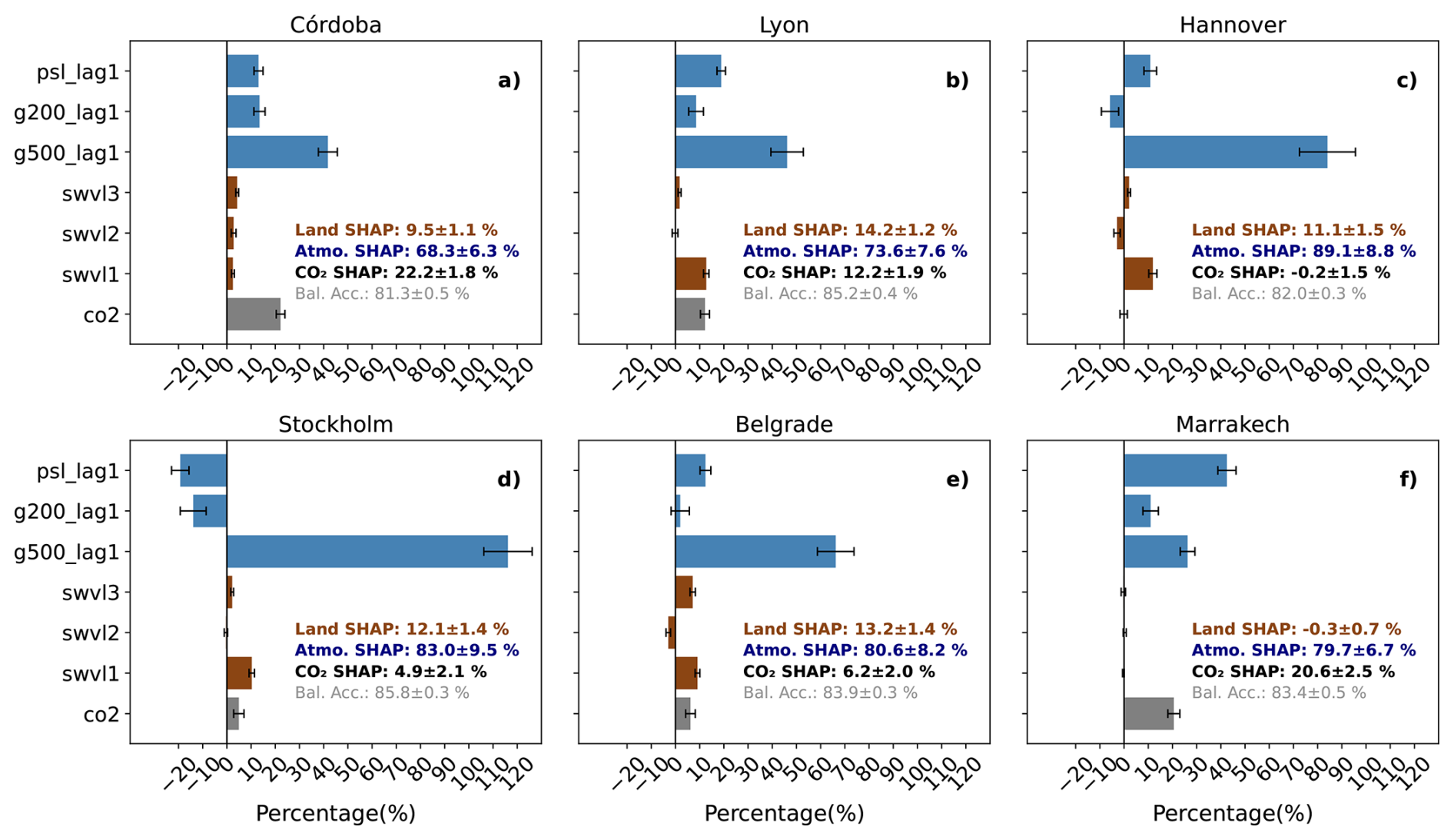
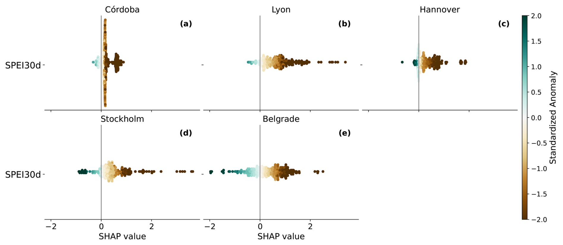
Figure D3 Same plot as in Fig. 6 but for the model using E-OBS observational data and the SPEI 30 d index as a proxy for the soil moisture feature.

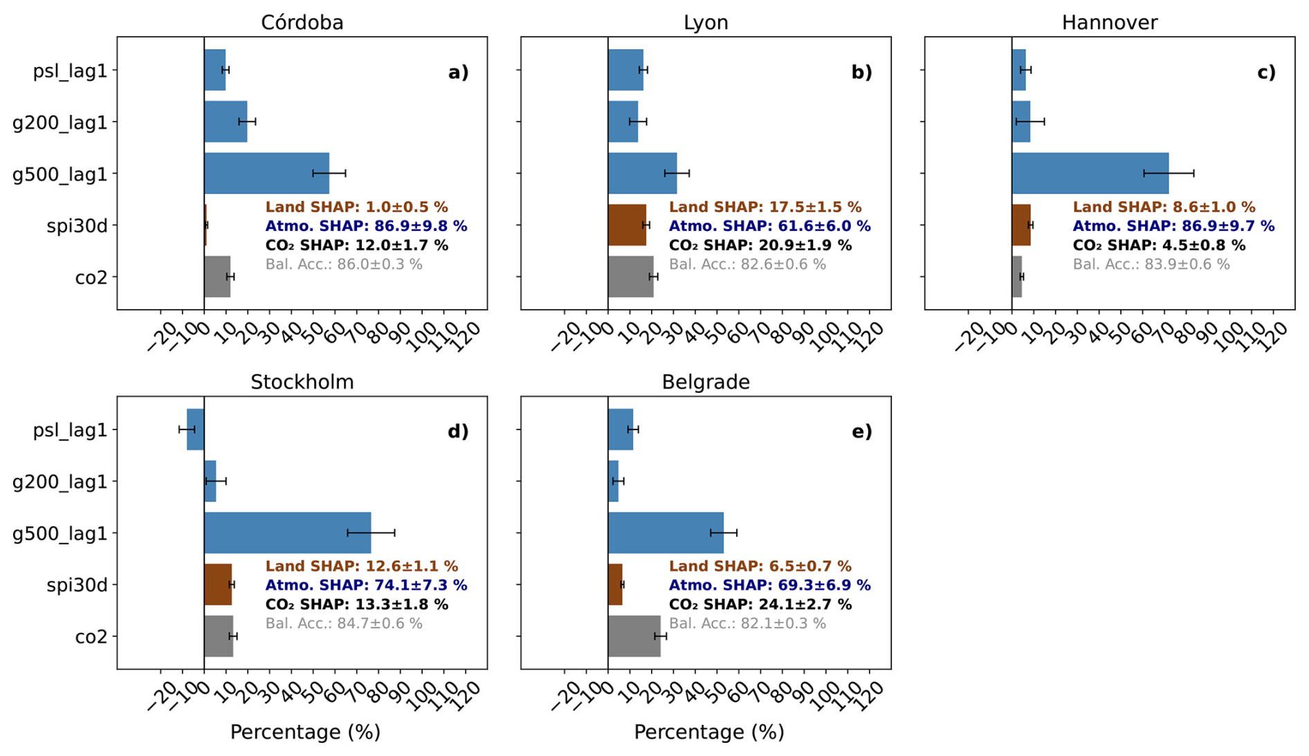
Figure D4 Same plot as in Fig. 5 but for the model using E-OBS observational data and the SPI 30 d index as a proxy for the soil moisture feature.

Figure D5 Same plot as in Fig. 5 but for the model using only g500 in the atmospheric circulation features.