Global shifts in mountain wave turbulence within high resolution climate models

Using a multi-model approach, this paper quantifies global changes in moderate or greater mountain wave turbulence (MWT) within a high-end warming scenario by 2050. We first show that simulated MWT changes depend on model resolution and therefore select three high resolution global climate model experiments for further analysis; HadGEM3-GC3.1-HM (25 km), EC-Earth-3P-HR (36 km) and MPI-ESM1.2-XR (34 km). The wide model and index uncertainty across continental average projections lead to a sub-continental 28 area approach. Using this method, we determined MWT is projected to increase over North America as a whole but decrease over the Rocky Mountains. An increase in MWT is projected for other regions including the Antarctic, Greenland, Georgia, Azerbaijan and parts of Chile and Argentina. A decline in MWT is projected for the Alps, Atlas and northern and central Andes. We also explore the modelled relationship of 10 m wind speed and MWT production; there is a positive correlation between the projected changes of MWT and surface wind speed. The aviation sector should be aware of the future projections in MWT, particularly for regions where a large increase in MWT is projected, such as the Antarctic and Greenland.

1 Introduction

Mountains impact the atmosphere from increasing localised precipitation events to generating vertical and horizontal propagating atmospheric gravity waves. Mountain waves grow, as they travel into higher altitudes with lower air density (Kim et al., 2018), steepen and eventually overturn breaking down into turbulent flow around the tropopause. The tropopause is a boundary between the troposphere and stratosphere with enhanced turbulent mixing of ozone, water vapour and aerosols (Whiteway et al., 2003; Lane et al., 2009) at 9–17 km above the surface. This is an altitude often used by cruising aircraft, a segment of the flight where passengers and crew are commonly not wearing seatbelts (Kim et al., 2018). Mountain Wave Turbulence (MWT) is the most significant mechanisms that impacts aircraft safety near mountains (Lane et al., 2009). In general, atmospheric turbulence has a dangerous and damaging cost on the aviation sector. Delays, injuries and fatalities have a huge economic loss worth millions of US dollars a year (Wolff and Sharman, 2008). Types of upper-level turbulence are defined by the features which develop them, for example turbulence that develops in vertically deep convective cloud is referred to convectively induced turbulence (CIT) (Wolff and Sharman, 2008). MWT, unlike in-cloud CIT, is not detectable by on-board RADAR equipment (Sharman and Lane, 2016). Here CIT relates to in-cloud formation, not near-cloud turbulence (NCT) which can develop from 5 to 200 kms away from active convective systems (Chun and Kim, 2008). MWT can impact a flight with little warning, leading to serious injuries and damages. Clear Air Turbulence (CAT), coined due to its formation without any convective features, is also not delectable. CAT often forms in the presence of an upper level frontal system, a jet core or jet stream. MWT and NCT are often included within CAT, due to their cloud-free, stratified development (Clark et al., 2000).

Global tropospheric warming has an impact on the frequency of CAT production in both observations and projected modelled data, with a global increase concluded in several studies (Williams and Joshi, 2013; Storer et al., 2017; Kim et al., 2023; Prosser et al., 2023; Smith et al., 2023; Foudad et al., 2024). Upper-level jet streams are shifting in speed and momentum with global temperature gradients altered, resulting in an increase in CAT production. However, new areas of research are trying to quantify the impact of global warming on MWT. Any future change to MWT will be equated to a shift in low level wind speed or a change in upper-level dynamical features suppressing or energising the breaking of inertial gravity waves. Kim et al. (2023), using a high-end SSP climate scenario, investigated the change in MWT between 1970–2014 and 2056–2101. Their paper used 14 different diagnostics to represent MWT within model data, with several indices and regions projecting an increase in the probability of encountering strong turbulence. The regions with a decline in MWT also had near-surface winds projected to weaken in time. Observations have shown a global slowing in surface winds over previous decades, referred to in literature as terrestrial stilling (TS). Despite TS shifting with several modes of climate variability (Zeng et al., 2019), it is projected to continue in many areas of the globe, including the Northern Hemisphere (NH) mid latitudes, in both middle to high warming projections (Deng et al., 2022). Kim et al. (2023) overall found an increase in MWT over two thirds of the globe, with large variations over the tropical regions.

Global climate models (GCM) are commonly used to investigate the changes in CAT and MWT in time (Williams and Joshi, 2013; Storer et al., 2017; Kim et al., 2023; Prosser et al., 2023; Smith et al., 2023; Foudad et al., 2024; Kim et al., 2023), with GCMs turbulence representation in the atmosphere as capable as re-analysis data (Williams and Storer, 2022). The spatial and temporal resolution in a GCM is an advantage, compared to, for example, verbal pilot reports (PIREPs). Aircraft encountering turbulence are required to record the time, location and severity of the event (PIREPs). PIREPs datasets are effective for turbulent climatology research but are not always reliable in their location or timing (Gill and Buchanan, 2018), with median uncertainties of around 50 km horizontally, 70 m vertically and 200 s temporally out (Sharman et al., 2014, 2006). The latest phase of Coupled Model Intercomparison Project (CMIP6) has a subsection of high resolution GCMs (HighResMIP) developed purely to investigate global meteorological dynamical processes and to bridge the resolution gap between numerical weather predictions (NWP) and climate models (Haarsma et al., 2016; Smith, et al., 2023). To test the capability of these HighResMIP models, and to add to Kim et al. (2023), our project explores global and seasonal MWT trends between 1950 to 2050, and the uncertainties and differences that can arise using a multi-model approach. Due to the surface wind speed findings in Kim et al. (2023), we too explore if shifts in wind speeds are the cause of projected MWT variations over the 101-year study period. Our next section, the methodology, discusses models and indices used to diagnose MWT, and all data processing techniques. Next comes our results and discussion and finally concluding remarks. The model and index uncertainties are highlighted in the continental analysis in Sect. 3.2 of the results, with a multi-model and index mean used for sub-continental, mountain range dependent analysis (Sect. 3.3).

2 Methodology and Data

2.1 CMIP6 HighResMIP global climate models

MWT is difficult to forecast, with the theory very well understood, but complicated to capture due to its small scale nature (Gill and Stirling, 2012). Within this paper, we make the assumption that large scale eddies will eventually cascade down the inertial sub-range into micro-scale sizes and into turbulent kinetic energy (Lester, 1993; Sharman and Lane, 2016), allowing us to use a range of model resolutions for this investigation. Our study uses a multi-model approach with 3 GCMs spanning 7 horizontal grid size domains. All models are part of CMIP6 HighResMIP simulations (Haarsma et al., 2020). These GCMs are HadGEM3-GC3.1, with 3 domains available (-HM; 25 km, -MM; 60 km, -LL; 135 km) (Roberts et al., 2019), MPI-ESM1.2 with 2 domains (-XR; 34 km, -HR; 67 km) (Gutjahr et al., 2019) and EC-Earth with 2 domains (-3P-HR; 36 km, -3P; 71 km) (Haarsma et al., 2020). The finer sub-models may start to resolve patches of turbulence, which climatology suggests are around 60 km wide and 1 km deep (Sharman et al., 2014). Due to this 1 km vertical depth, we focus on the model horizontal resolution, with thickness representation currently unattainable on our modelled vertical levels. These finer horizontal resolutions are used for the majority of the paper, discussed further in Sect. 3.1. This study uses the historically forced coupled climate and ocean experiments (1950–2014) with the future projected forcing of 2015–2050, simulating the high end SSP8.5 scenario (Haarsma et al., 2016). The benefits of using these CMIP6 GCMs relates to the global variability of our data, and the finer spatial resolution (relative to other global models). There are some limitations such as the smoothed topography limiting our ability to detect the complex MWT generation. This limitation means that not all MWT prone zones, found through observations, are detected by our approach (Fig. 1). This issue is also related to our dependency on terrain gradient discussed next. Our approach is done to explore the capability of our models, but future work could apply NWP modelled terrain to quantify further complexities.

Figure 1 Areas of the globe in which our GCMs project MWT, averaged over three GCMs; HadGEM3-GC3.1-HM, MPI-ESM1.2-XR and EC-Earth-3P-HR, across all indices; MWT_FD, MWT_FDWS, MWT_WS, MWT_HTG, MWT_FF, MWT_DIV.

2.2 Diagnosing turbulence

To diagnose regions of turbulence, a number of indices, linked closely to atmospheric instability, are applied to our CMIP6 GCMs simulations. MWT and CAT share similarities in their formation, so previous literature has applied CAT indices to represent MWT in the atmosphere. Sharman and Pearson (2017) and Kim et al.(2023) combine CAT diagnostics with certain surface and terrain variables to create an index that just represents MWT;

$${\text{Index}}_{\text{MWT}}={\text{Index}}_{\text{CAT}}\times \text{Ds}$$

Ds is a non-zero near-surface element that's model and index dependent. Within this paper, Ds = surface height (> 200 m) multiplied by both terrain gradient (> 0.5 km m⁻¹) and maximum low-level wind speed (< 1 km). Ds values differ across each model, with terrain gradient model dependent. Sharman and Pearson (2017) determined, through experimentation, that these three variables within Ds combined with a CAT diagnostics represented MWT effectively. Kim et al. (2023) tested using vertical velocity within Ds, instead of low-level horizontal wind speed, but found a poorer statistical evaluation. This method of calculating MWT was deemed skilful against PIREP data, in comparison to a orthographic gravity wave parametrisation scheme (Kim et al., 2018). In our study, we apply six indices used previously to diagnose the presence of CAT (Williams and Joshi, 2013). These CAT indices are horizontal temperature gradient (HTG), frontogenesis function (FF), the divergence of horizontal wind (DIV), 200 hPa wind speed (WS), flow deformation (FD) and finally a combination of flow deformation and wind speed (FDWS). Each MWT index is denoted with the subscript of their CAT index contributions, for example MWT_HTG is the product of horizontal temperature gradient and Ds. Sharman and Pearson (2017) found that these 6 indices, with 8 others, are very well at representing MWT at high altitudes and particularly good at avoiding false alarms situations, with a probability of detection for non-events (PODN) at 98.9 %. Horizontal temperature gradient (combined with Ds) on its own also has a PODN 99.1 %. However, Sharman and Pearson (2017) only focuses on the contiguous united states of America (CONUS).

Following recent MWT literature (Kim et al., 2023), our study assumes moderate or greater (MOG) turbulence is arising globally at the 98th percentile value of each index and focuses on the atmospheric pressure of 200 hPa (native vertical levels from projections). These threshold values are index but also model, and ensemble member dependent. Further information found within Appendix C. To statistically determine the change in projected MWT, our results use a linear regression fit, with a confidence interval of 95 %. Trends that do not meet this confidence interval are removed from the multi-model and index averages. As an extra research question, this paper looks at the average and maximum 10 m wind speeds for participial regions to explore TS in our models. Since our analysis is related to the change in MWT over the century, using both the average and maximum helps equate the general trend in time (average) and if there are more instances of rapid wind speeds that lead to further MWT generation (maximum). Within results Sect. 3.3, MWT variations in 28 regions of the globe are investigated. These zones were picked through initially exploring areas in which MWT arose, and further breaking down these areas into zones that generally projected one trend in time.

3 Results and Discussion

As discussed, terrain height and gradient are applied to CAT indices to identify MWT. The importance of terrain gradient is highlighted effectively in Fig. 1, which portrays the areas where our models diagnosed MWT. Regions of the globe with large plateaus, such as Greenland and the Tibetan Plateau, are enclosed by areas of MWT with these steep slopes dominating. As expected, MWT is most prominent over large mountain ranges, such as the Andes, Rocky and Himalayas.

3.1 Two decade comparison

The MOG MWT decadal difference between 1950–1960 and 2040–2050 is displayed within Fig. 2. Here this relative change in MWT is shown for all models domain sizes averaged across the six indices. A definitive lack of detail is evident within mid-range/coarser sub-models, clearly shown by HadGEM3-GC3.1-LL (Fig. 2i) with few MWT zones. PIREP analysis suggests that there are considerable more regions where aircraft have experienced MWT (Sharman et al., 2014), for example North America projected MWT is non-existent within this 135 km grid spaced model. Our coarser models fail to represent MWT in several locations, with a key limiting attribute our terrain gradient threshold and the unfortunate smoothing of terrain implemented in climate models. This creates a model resolution criterion for our MWT analysis. It may differ in other studies that imported terrain from a NWP model, but our study is to highlight the uncertainties on representing MWT in GCMs. Interestingly, the mid-range sub-models project similar MWT changes, when compared to their finer counterparts. This is shown effectively within Fig. 2g and h, which display the average across the models, regridded to 36 and 71 km, respectively. Both subplots have a separate steep increase or decrease over Greenland and northern South America. However, there are differences in the amount of “white” patches, which simply project “no-change” but the occurrence of MWT. The agreement across model resolutions, adds weight to the confidence in MWT projections, however, due to the increase detail in fine grid domain models, this paper progresses with the three finer models shown in Fig. 2a, c, and e.

Figure 2 Decade difference in MWT between 1950–1959 and 2040–2049, for all seven resolutions; HadGEM3-GC3.1-HM 25 km, -MM 60 km (a, b), -LL 135 km (i), EC-Earth-3P-HR 36 km, -3P 71 km (c, d) and MPI-ESM1.2-XR 34 km, HR- 67 km (e, f). Subplots (g, h) show average across finer and mid-range GCMs. Conservative regridding method, modifying data into 36 and 71 km across the finer and mid-range domains.

3.2 Continental index and model variability in seasonal MWT projections

This section explores the variability in the three modelled projections, and the MWT index uncertainty, over each continent. Tables 1 and 2 discuss all seven continents with Figs. 3–5 showing results for North America, South America and Asia. These figures have also been repeated with the remaining continents and can be found in the Appendix. For clarity, insignificant linear regression trends (less than a 95th confidence level) within season or model are greyed out of figure legends. All four season are individually processed, with a final annual yearly median taken and plotted. As expected, all annual averages reside in the middle of their seasons. These results focus on the change each year in MWT compared to a global threshold for MOG (98th percentile) turbulence found using all years (and seasons) with the 1950–1960 decade. Using a global threshold provides information on the most turbulent projected regions of the globe, evident through analysis of the y axis in all subplots in aforementioned figures.

Table 1 Seasonal and annual median slope values across each GCM, including standard deviation for medians and ranges for North and South America, Europe and Africa. The number of statistically significant positive slopes, at 95 % confidence interval, are highlighted in bold.

Table 2 Seasonal and annual median slope values across each GCM, including standard deviation for medians and ranges for Asia, Australia, and Antarctic. The number of statistically significant positive slopes, at 95 % confidence interval, are highlighted in bold.

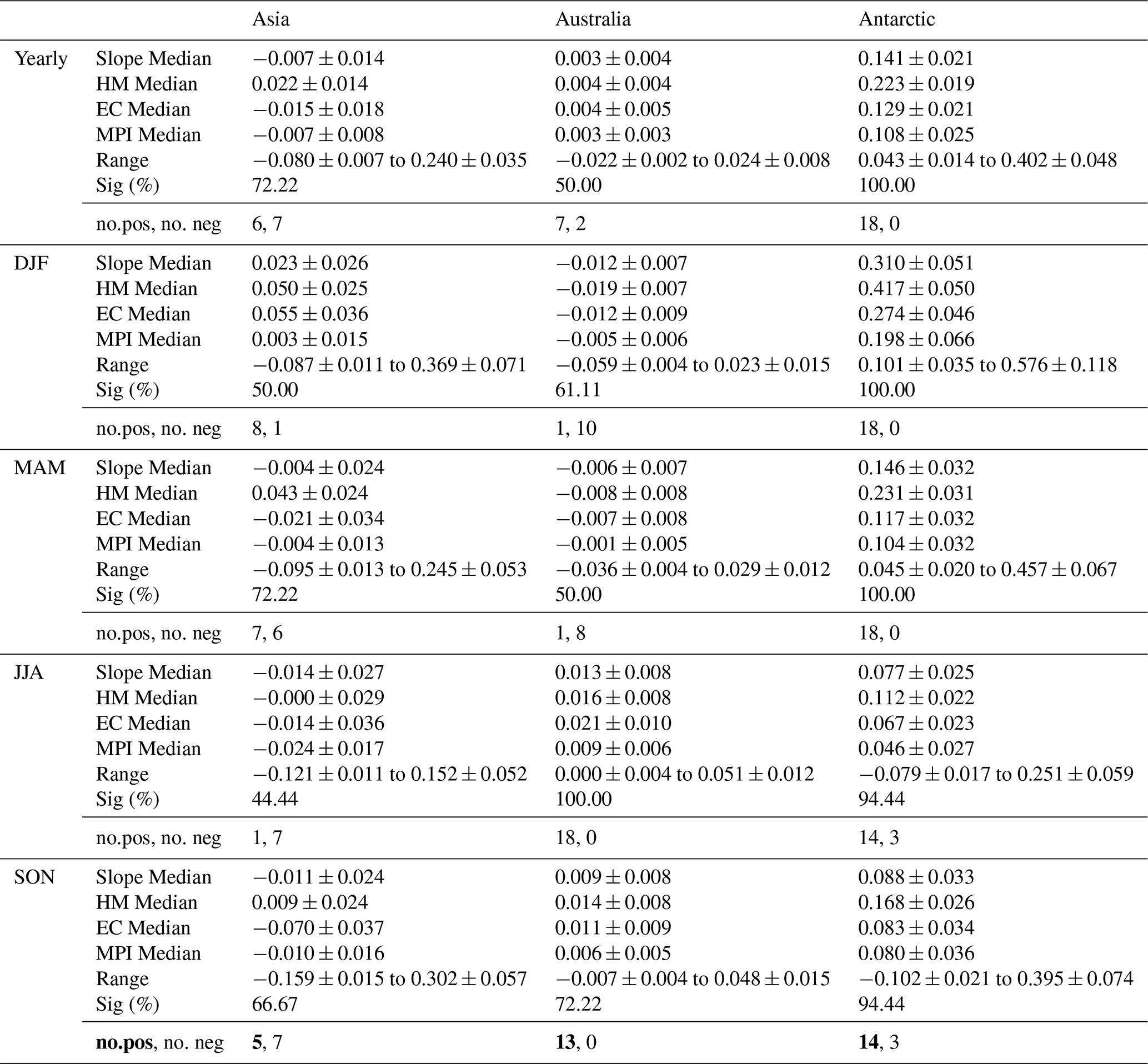
Figure 3 Line plots of relative percentage change over North America for each year and season compared to a 1950 decadal global references, for each GCM; HadGEM3-GC3.1-HM, EC-Earth-3P-HR, and MPI-ESM1.2-XR and for each individual index. Line colour and marking differ for each season, with DJF blue and dashed, MAM green and dash dotted, JJA red and soild, SON purple and dotted. Annual change, which includes all seasons is black and solid.

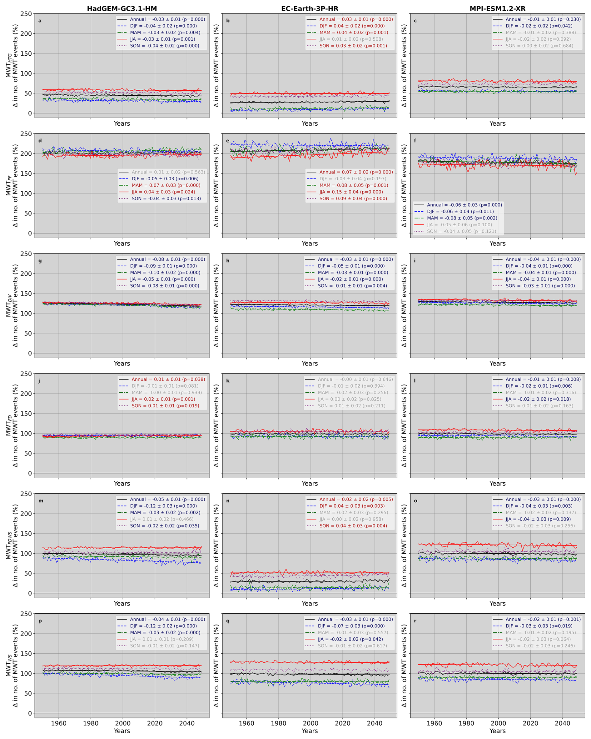
Figure 4 Line plots of relative percentage change over South America for each year and season compared to a 1950 decadal global references, for each GCM; HadGEM3-GC3.1-HM, EC-Earth-3P-HR, and MPI-ESM1.2-XR and for each individual index. Line colour and marking differ for each season, with DJF blue and dashed, MAM green and dash dotted, JJA red and soild, SON purple and dotted. Annual change, which includes all seasons is black and solid.

Figure 5 Line plots of relative percentage change over the Asian continent for each year and season compared to a 1950 decadal global references, for each GCM; HadGEM3-GC3.1-HM, EC-Earth-3P-HR, and MPI-ESM1.2-XR and for each individual index. Line colour and marking differ for each season, with DJF blue and dashed, MAM green and dash dotted, JJA red and soild, SON purple and dotted. Annual change, which includes all seasons is black and solid.

This paper includes Greenland within North America. Greenland has large increases in MWT, evident in Figs. 2 to 3 and within Sect. 3.3 where it is discussed further. This may skew an increase in MWT within this sub section, with variability across North America previously shown. There are seasonal differences in the amount of projected MWT in North America, with a comparably large amount in DJF (December, January, February) within Fig. 3's HadGEM3-GC3.1 and EC-Earth-3P subplots. This is expected with NH winter favourable for MWT generation over USA and Canada, with lowered tropopause heights and peak surface westerlies crossing mountain ranges perpendicularly (Guarino et al., 2018). MPI-ESM1.2 DJF and SON (September, October, November) projections are similar in MWT_FD, MWT_FDWS, MWT_WS within Fig. 3, with DJF at times below that of SON and other seasons. A double peak in maxima has been shown in some climatology MWT North America studies. Wolff and Sharman (2008), using PIREP data to find trends in MWT on the United States of America, found peaks in DJF and NH spring (MAM; March, April, May) but not necessarily SON.

Over North America, our three high resolution models agree strongly that MWT has increased over the 101-year period, with an average over all seasons at 0.063, 0.05 and 0.046 % yr⁻¹ for HadGEM-GC3.1-HM, EC-Earth-3P-HR and MPI-ESM1.2-XR. These slopes, and other for each season and continent can be sourced from Table 1. This projected increase in MWT was evident in all but two indices, with MWT_HTG and MWT_FDWS SON projecting a drop in MWT. Apart from these two slopes there is good agreement across the indices and a similar trend across seasons. There are some seasons that have a greater number of significant slopes (p<0.05) than others. For example, North America MAM only has 4 significant slopes, whereas SON has 13 (11 increase, 2 negatives; Table 1) and the largest average slope of 0.08 % yr⁻¹ which equates to 8.08 % over the projected period.

The annual and seasonal percentage changes in MWT over South America are displayed in Fig. 4. Index variability is clearly visible within this figure (y-axis spread), with MWT_FDWS (Fig. 4n) values around the 0 %–50 % range and MWT_FF around the 180 %–250 % range (Fig. 4d–f). This means the indices project a different amount of MWT over the region and are not capturing similar MWT generation situations. This is not an issue, as the purpose of using 6 indices is to capture the many situations in which MWT may occur, but interesting that this is evident within the South America projections. The remaining diagnostics sit at around +100 %. This is an index variation, rather than a model disagreement, with all models preforming similarly. However, models do differ on trends over the period, for example MWT_HTG decreases in HadGEM-GC3.1-HM (Fig. 4a) but increases in EC-Earth-3P-HR (Fig. 4b) and in MWT_FDWS there is a decreases in HadGEM-GC3.1-HM (Fig. 4m) and MPI-ESM1.2-XR (Fig. 4o) yet an increases again in EC-Earth-3P-HR (Fig. 4n). The projected trends, over South America, differ across the seasons, models and indices. On average, a decrease in MWT is projected for South America, with the largest decline (with a high number of slopes, 13:2) in DJF (SH summer) by 0.044 % yr⁻¹ or 4.44 % over the period.

Due to the Himalayan Mountains and many other steep mountain ranges over Asia, the MWT percentages on the y axis in Fig. 5 are the largest compared to any other continent. The seasonality of MWT is very interesting over Asia, with different indices projecting MAM, JJA or DJF to have the maxima in MWT across their retrospective subplots. Further explored in our regional analysis (Sect. 3.3). Interestingly, MPI-ESM1.2-XR projection are all around 150 % (y axis) no matter the index, whereas there’s a wider spread across the seasons and indices for the remaining models. In terms of trends over the period there is a mix depending on season, index and model. For MWT_HTG, strong model agreements that a decrease in MWT is evident in all seasons but DJF. Again high model agreement in MWT_DIV. There is high confidence in the JJA and DJF projections with 8:1 (positive:negative) and 1:7 slopes over Asia (Table 2). Overall, an increase in MWT is projected for DJF over asia, and a decline is projected in JJA by 0.023 and −0.014 % yr⁻¹, respectively.

Europe's MWT rates are much smaller than over Asia or South America, and so the MWT percentages are often negative (Appendix B). The projected trends in Europe are strongly index dependent, despite robust model agreement (excluding MWT_FDWS). The index variation leads to competing slopes and low overall-multi-model projections. The number of confident slopes is relatively small compared to the other continents with only one index (MWT_HTG) significant in MPI-ESM1.2-XR projections. Summer in Europe (JJA) had the highest relative percentage of significant slopes with a decline average of −2.323 %. by the end of the 101-year period.

Over Africa, a similar index dependent picture as previously seen in South America (Fig. 4), develops for the amount of MWT. With MWT measures ranging from −75 % in MWT_FDWS, −50 % in MWT_FD, −25 % in MWT_WS, MWT_DIV, MWT_FDWS and +50 % in MWT_FF. The amount of projected MWT in Africa is similar to that in Europe (highlighted in appendix). For trends over the period, like Europe, a general decrease in MWT develops, however with more confident negative slopes. A clear decline in DJF, JJA and SON with a mix in MAM. Strong model agreement within this continent, with largest variation due to index differences. It should be noted that strong model agreement is only between EC-Earth-3P-HR and HadGEM-GC3.1-HM, with MPI-ESM1.2-XR results all insignificant. This could be due to the number of ensemble members within this simulation. As mentioned in our methods, only 1 ensemble for this run is used.

A strong seasonal response arose in the slopes over the Australian continent, with a clear decrease in MWT over DJF (1:10; positive:negative slopes) and MAM (1:8) and an evident increase for JJA (18:0) and SON (13:0) (Table 2). In fact, JJA has strong model and index agreement with all producing significant increasing trends with an average of 0.013 % yr⁻¹. SON too has a very similar agreement and trend but a lower number of significant slopes, at 72.22 %. For the remaining seasons, there is good model and index agreement on trend with just MWT_FF EC-Earth-3P-HR projections projecting an increase in DJF and MAM MWT, with all the rest suggesting a decline. The Australian continent does not have a high amount of projected MWT compared to the others and is the least turbulent modelled continent in this study.

There is a clear seasonality in the amount of MWT over the Antarctic, with JJA and DJF being the most and least turbulent season. The large JJA (winter) MWT values place this continent second, after Asia, with the amount of projected MWT with the GCMs. Within this figure, only 6 projections suggest a decrease in MWT with 3 lines in JJA and 3 lines in SON across MWT_HTG and MWT_FDWS projections. Despite this, there is quite strong model and index agreement, with all other indices, across all GCMs, projecting a significant increase in MWT. The greatest increase is evident in DJF projections with a large rise of 0.31 % yr⁻¹ or 31.3 % over the 101 year period. Few airlines travel over the Antarctic but this result does put those few airlines at risk travelling, particularly in SH summer.

Continent summary

An overview of the slope distribution is highlighted in Fig. 6. As you can see the greatest increase in MWT is projected over the Antarctic by 0.52 % yr⁻¹ or 52.52 % over the 101-year period. The average is considerably lower at 0.14 % yr⁻¹. The average seasonal trend for each continent and the number significant positive trends vs negative slopes are listed below and above the box-plots. For the Antarctic, all seasonal averages project an increase in MWT, with a ratio of 82 to 6, positive to negative slopes found in Fig. 6. The second highest slope is the maximum trend over Asia at 0.31 % yr⁻¹, although on average, there is a decrease by −0.005 % yr⁻¹. This is due to the different seasonal trends, with a decrease in JJA and SON and a rise in DJF and MAM. North and South America and Europe have a similar maximum slope of 0.16, 0.15 and 0.17 % yr⁻¹, respectively. Over the three interestingly, the largest decrease in MWT is evident in Europe at −0.18 % yr⁻¹ and then in South America at −0.12 % yr⁻¹. With North America minimum (−0.04 % yr⁻¹) in the same range as Africa (−0.09 % yr⁻¹) and Australia (−0.052 % yr⁻¹). The projected average changes in MWT for North America, South America, Europe, Africa and Australia are 0.032, −0.019, 0.004, −0.006 and 0.004 % yr⁻¹, respectively. These average shifts only equate to 0.4 % to 3 % over the 101-year period due to the large biases in averaging over such a wider area. To determine regional differences, our next section breaks down into sub-continental zones.

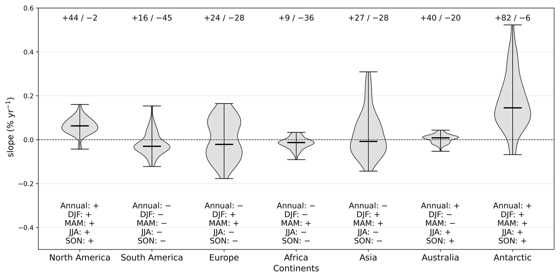
Figure 6 Distribution of all slopes for each continent (Figs. 3–5 and Appendix Figs. B1–B4), with the number of positive or negative significant (at 95th confidence level) slopes written above each violin plot, and the overall trend of slope (i.e. positive or negative) for each season written below each plot.

3.3 Multi-model mean MWT regional analysis

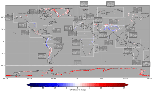
The projected MWT trends across 28 sub-continental regions are highlighted in Fig. 7. This figure shows the difference between 1950–1960 and 2040–2050, as done in Fig. 2, averaged over the GCMs and indices. The maximum, mean and minimum % of MWT over the 101 year period, relative to the 1950s decade (same as Sect. 3.2) for each region is also displayed within this figure. The linear fit slope over each region can be found in Fig. 8.

Figure 7 The map is coloured by the difference between the first decade of our period 1950–1960 against our final decade 2040–2050. The boxes are used to highlight the 28 sub-continental regions used within our analysis. The textbox show the average, min and max amount of MWT in percentage (relative to global 1950's decade) within each box.

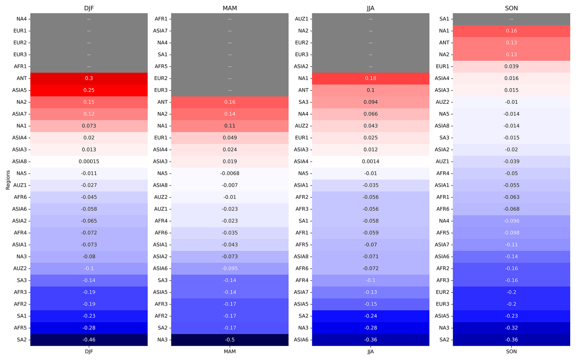
Figure 8 For each of our 28 regions, the linear regression slope between 1950 to 2050 for each season is displayed, with an average taken over the three high resolution GCMs; HadGEM-GC3.1, MPI-ESM1.2-XR and EC-Earth3P-HR. The area in which each region represents is found on Fig. 7.

The Antarctic, as clearly shown in Figs. 7 and 8, is a region of the globe with a relatively significant increase in MWT, at most by 0.3 % yr⁻¹ in DJF. This increase is evident in all models but particularly in HadGEM3-GC3.1. The average amount of projected MWT over the Antarctic, across the indices, is just greater than the Alps (EUR2) and around a similar range as found in SA1 over the north Andes. This is highlighted within Fig. 7, with the max, mean and min percentage of MWT over the period. These boxes help to infer the projected most turbulent regions, compared to our global threshold. The regions with the greatest amount of turbulence are ASIA6 over the Himalayas, SA3 over the southern Andes, ASIA5 over Turkey and the middle east and then NA3 over the Rockies (Fig. 7).

There are two notable regions in North America, NA1 and NA2, that project a large rise in MWT across all seasons (Fig. 8). The North American continent is broken down into five regional areas. Region NA1 covers Greenland, Iceland and Canada north to north-east of the Hudson Bay. Aircraft are known to travel through this region, particularly over southern Greenland, when flying from Europe to North America and vice versa (Lane et al., 2009; Doyle et al., 2005). MWT formation over Greenland is often associated with the passage of a surface cyclone, due to progression of easterly or south easterly wind flow over the mountain’s terrain, with 40 % of all significant turbulent events linked with this type of generation (Lane et al., 2009). NA1 is the second most turbulent region in North America. Greenland is a known turbulent region of the globe, with every fourth day having at least one MOG turbulent PIREP (Lane et al., 2009). In terms of seasonality, literature suggest MWT frequency is like contiguous United States (CONUS), where some winter months (January) have had rates four times the amount of MOG MWT compared to spring months (May) (Lane et al., 2009; Wolff and Sharman, 2008). Once averaged over all GCMs and indices (Fig. 8), it’s a projected increase of 18.2 %, 16.2 % 11.1 %, 7.4 % for JJA, SON, MAM and DJF over the period (1950 to 2050).

NA2 covers central and western Canada and Alaska has a larger relative increase in MWT compared to the rest of the globe, with an average increase of 15.2 % (DJF), 14.1 % (MAM), 13.1 % (SON). Insignificant trends over the period for JJA. NA3 covers part of the Rocky Mountain range and is the projected most turbulent (mountain generated) region of North America (+648 % at max, Fig. 7). The Rocky Mountains are a well-documented turbulent area with MWT the major source of turbulence over the western half of the USA (Wolff and Sharman, 2008). This papers limitations in terrain gradient resolution means only parts of the Rocky Mountains are represented. This has unfortunately lead to key areas in the western US, which have been found to be very turbulent (Kim et al., 2019; Park et al., 2016), not represented within our paper. This should be taken into consideration when referencing results. In contrast to the other North America regions, there is a projected decrease in the amount of MWT over NA3 with DJF, MAM, JJA and SON −8.1 % −50.5 %, −28.3 %,-32.3 %. This significant decline MAM is the greatest decrease globally of all our projected trends.

The 2nd greatest global decrease is found in South America in SA2 in DJF by −46.5 %. Within this region, all other seasons follow this trend decreasing by −17.2 %, −24.2 %, −36.4 % in MAM, JJA and SON. There are three regions in South America shown in Fig. 1, that break down the Andes mountain range into northern (SA1), central (SA2) and southern (SA3) sections. Findings suggest the southern parts of the Andes in SH winter (JJA) could become considerably more turbulent. Figure 7 shows the difference between 2050 and 1950, and highlights an evident MWT increase for SA3 for all seasons. However, this is decadal variability, as the trend over the century only projects JJA to increase in MWT by 9.5 %. Such an increase may seem relatively small, compared to other slopes, but it is already the second most turbulent region of the study (mean of 670.4 %, Fig. 7). The remaining seasons in SA3, and all within SA1 and SA2 project a decrease in the amount of MWT.

The 3rd greatest global decrease in MWT is within Asia in ASIA6, with a drop of −36.4 % over the century in JJA. Over Asia, eight zones were chosen for further analysis with ASIA6 encompassing Indian and Sri Lanka. Note that some regions have parts of Europe and the Australian continent within them. The remaining seasons too project a drop in MWT for AISA6 but by considerably lower amounts with −5.7 % in DJF, −9.6 % in MAM and −14.1 % in SON. The largest amount of projected MWT is found in Asia in zone ASIA4. This area includes the Himalayan mountain range and Tibetan plateau within it. There are disagreeing trends across the model projections for this region. One should take a moment to notice that despite a decrease in decadal difference between 1950 and 2050 (Fig. 7), a trend over the period is increasing by a small amount of 2 %, 2.4 % 1.4 % and 1.6 % in DJF, MAM, JJA and SON. This is due to EC-Earth-3P-XR projecting a significant increase and monopolising the average trend, despite two out of the three projecting a decrease.

ASIA5 and ASIA3 are the 2nd and 3rd most turbulent regions in the Asia. ASIA5, which covers Azerbaijan, Georgia, Turkey and parts of Iran, Kazakhstan and Turkmenistan, has a relatively large increase in MWT over DJF with a 25.3 % projected rise from 1950 to 2050. Despite this rise, a decline is projected for the remaining seasons by 1.4 % in MAM, −1.5 % in JJA and −23.3 % in SON. Clear seasonal dependence on the trend in time for this region. In contrast ASIA3, projects an increase in all seasons by around 1 %–2 % over the period.

AFR5 in Africa has joint 6th greatest decline (joint with NA3 in JJA) with a drop of −28.3 % in DJF. Africa is split into six regions, with AFR1 slightly cutting off the bottom of Spain and Italy but primarily covering Morocco, Algeria, Tunisia and Libya. AFR1 is technically projected most turbulent region in Africa, bur AFR3 is a close second. AFR3 includes regions in the Middle East (Asia). AFR2, AFR4, AFR5 and AFR6 have a much smaller amount of MWT compared to AFR1 and AFR3. A decrease in MWT is projected in all regions in Africa, in all seasons on average. EC-Earth-3P-HR projects an increase in some regions, which wins the tug of war in trends for the decadal difference between 1950 and 2040 (Fig. 7), but not the overall trend (slope) over the century (Fig. 8). Kim et al. (2023) which did a similar study but using more indices, and different models, found a decrease in summertime MWT agreeing with our trend. However, this paper also found a sharp rise in wintertime MWT, differing to our projections.

There are three regions of Europe included in this sub-continent analysis. Only EUR1 projects an increase in MWT, with a shift of 2.5 %–5 % across seasons excluding DJF. Interestingly, there are no significant trends in time over winter across Europe. Please note that there are some European countries included in the Asia overlap, due to wide boxes. EUR1 covers the Scandinavian counties, with this increase arising around the Scandinavian Peninsula (Scandes) and over Svalbard. Another region of interest is EUR2 which covers the Alps, the Pyrenees and Apennines mountain ranges. Results are only significant in SON, due to large variability in indices and models. A significant decrease of −20 % was projected in this climatology turbulent season.

There are technically three regions within the Australian continents, with ASIA8 covering both Asia and the Australian continent. AUZ1 and AUZ2 are located south of ASI8 over Australia and New Zealand. AUZ1, which includes areas in the Australian country like New South Wales, Victoria and Tasmania has a slight decrease over the period by −1 % to −4 % over all seasons. There are greater season differences in AUZ2, which covers New Zealand. An increase of 4.3 % in JJA but a decline by −10 % in DJF, −2.3 % in MAM, −1 % in SON. Interestingly, the amount of MWT in this box is greater than many regions in Asia and Africa.

Figure 9 The average and maximum low-level wind speed trends within each region. Highlighted in red and blue if change in wind speed is the same as shift in MWT within the same area.

As is highlighted clearly on Fig. 8, there are more places in the globe projecting a drop in the MWT than increase. Kim et al. (2023) projected an increase in MWT in the mid to high latitudes and a decline usually in the Tropics. This is somewhat the case within our projections, although South America and the Rockies project a decline in line with the tropical regions. Kim et al. (2023) found that their changes in MWT were linked to low-level wind change. Figure 9 shows if any regions have a similar confident trend in time for both MWT projections and mean or maximum 10 m wind speed variation in time. The Antarctic trends in DJF and JJA are linked to an increase in the average and maximum low-level winds. The British Antarctic Survey found surface winds strengthen by 15 % since 1980. The mean JJA winds and maximum SON winds over NA2 are increasing over the period, this agrees with our change over Canada and Alaska. Over North America, the decrease in MWT over the Rockies in SON is linked to a decrease in the maximum wind speeds. The decrease over India and Sri Lanka is also associated with the decrease but in the average low-level wind. The choice to include the average and maximum wind speed was done to encapsulate if the wind speed on average was increasing, rather than just if the number of maximum wind speeds increased.

4 Conclusions

Using three HighRes-MIP CMIP6 GCMs, this study investigated the modelled projections of global MWT turbulence over a 101-year period. Through an initial comparison between the 1950–1960 and 2040–2050 decade, we found coarser models could not detect as much detail as their finer counterparts. This was linked to improved gradient and terrain height information. This study continued only with three higher resolution models; HadGEM3-GC3.1-HM (25 km), EC-Earth-3P-HR(36 km) and MPI-ESM1.2-XR (34 km). Each MWT index was broken down and analysed initially through continental yearly analysis (Figs. 3 to 9). Regional dependencies arose around model and index agreement, with seasonal components an important contributor to results. Finally, a sub-regional approach was discussed, where seasonal MWT and surface wind speed trends were analysed.

On average, the North American continent had an increase in MWT. However, a lot of the trends in time were not significant. On further sub-continental analysis, the zone encapsulating the Rocky Mountain range was shown to be decreasing in the amount of MWT in all seasons. Greenland, a region used often for transatlantic travel, had increased in the amount of MWT, with its greatest shift in JJA by +18.2 %. Over South America, a decrease in MWT was evident from initial analysis. This decline in MWT continued into further sub-continental analysis, with strong model agreement on northern and central regions of the Andes projecting a decline. Southern Andes projects an increase in SH winter by 9.5 % but over remaining seasons a decrease was evident.

This decrease in projected MWT continued across Africa, with the greatest decline over the Madagascar in DJF by 28.3 %. Strong agreement across all seasons for a decline in MWT over this continent. In comparison, Europe's projections suggested a decrease in just one region covering the Alps and other central European mountain ranges in MAM. MAM was the only season with a significant trend in time, this was due to a wide spread of index and model trends. However, a rise in MWT evident in Scandinavia and the Arctic circle in Svalbard.

An increase in MWT was projected in one model over the Himalayan mountain range and Tibetan plateau (region; ASIA4) which lead to an on average increase in MWT. However, the remaining two projected a smaller relative decline. This is a limitation of the final summary results in our sub continental results, with averages over models and indices taken. As discussed in our continental review, there are often disagreements between GCMS and the methods to diagnose MWT.

Limitations and future work

This paper acknowledges that modelled atmospheric and ocean data is used, with all projections based on a future SSP-8.5 scenario. This is an extreme climate warming scenario with no action, little mitigation or adaptation (Deng et al., 2022). As discussed in methodology, one limitation within previous work (Sharman and Pearson, 2017; Kim et al., 2023) that continues within this paper is that MWT often occurs downstream from mountain ranges (Wilms et al., 2020). Our region should encapsulate source of the downstream MWT due to our inclusion of slope gradient, but may miss MWT which travels far distances due to certain meteorological conditions (Lane et al., 2009). Our terrain is sourced from our models, and not a secondary source with higher ground resolution. Future studies could apply such resolutions to fully capture other regions of MWT. Our 28 zones are based on regions within the continents that on average over time, model and indices had similar trends in time, so we could really see if these trends were apparent in each season, model etc. For future work, breaking down these zones into meteorological characterises that impact the area could be the next step, and may reduce some uncertainty in our results.

Appendix A: Breakdown into Indices; Two decadal comparison

Figures A1–A3 display the decade difference for HadGEM3-GC3.1-HM, EC-Earth-3P-HR and MPI-ESM1.2-XR individually, for each index, rather than averaged (Fig. 2). These figures also include the decade difference in daily maximum (Figs. A1g–A3g) and median (Figs. A1h–A3h) surface wind speeds. As mentioned in Sect. 2; Methodology and Data, low-level wind speed is a variable within our MWT indices. One area of investigation is to understand if a shift in MWT is linked to possible changes in surface winds. Deng et al. (2022), using different, coarser CMIP6 GCMs and observational data, found CMIP6 GCMs correctly reproduced the decreasing trends (between 1980–2010 and 2070–2099) in near surface winds in North America, Europe and East Asia. They did on average simulate faster wind speeds at coastal areas than inland, and have shown seasonal variations. Please note these wind speed percentage change only displays results over regions in which MWT arises, other areas excluded for ease of comparison.

Within the HadGEM3-GC3.1-HM (25 km) model, a general increase in maximum wind speed is apparent in Fig. A1g, with a larger percentage change compared to the change in average surface wind speed (Fig. A1h). The maximum surface winds have relatively large percentage shifts over Greenland, the Antarctic and Asia. These regional increases correlate the rise in MWT frequency in many indices within this figure. Interestingly, average wind speed has more regions that project decrease over the continents, than maximum wind speed, particularly interesting is the decline on the coastlines of the Antarctic between 60–180° E. One could argue the changes in wind speed, in both maximum and average, correlate to projected MWT percentage differences in such indices as MWT_FD, MWT_FDWS,MWT_WS. Within this figure, the projected outcomes from these indices are relative similar within the HadGEM3-GC3.1-HM model.

Interestingly, MWT_DIV (Fig. A1c) projects a very notable MWT decline across the globe, including southern Greenland, the North America Rocky, Central and Southern Andes and the Himalayas. A decline in maximum wind speeds arises over the Antarctic and north west Greenland, regions where MWT_DIV projects a drop in MWT frequency between the two decades. MWT_HTG (Fig. A1a) is an index shown to effectively represent MWT over North America (Sharman and Pearson, 2017). This index projects either no change or a decline in MWT over southern Greenland, USA and Canada. Despite similarities to MWT_DIV, MWT_HTG differs over the African and Asian contentment, with an increase in turbulence at the southern edge of the Tibetan Plateau. The most notable index within Fig. A1 is MWT_FF, with a pronounced decline projected over the northern Andes, eastern Africa, the Himalayas and Indonesia and a substantial increase projected in other regions of the globe. Except for similarities in North America, MWT_FF and MWT_HTG have almost opposite projections. A weakening in MWT_HTG projections may be associated with polar amplification weakening the meridional temperature gradient.

The EC-Earth-3P-HR (36 km) and MPI-ESM1.2-XR (34 km) too have the most notable change found within MWT_FF. These two models project a greater overall increase over Asia than HadGEM3-GC3.1-HM within this index. There is a notable drop in the number of regions producing MWT within MPI-ESM1.2-XR projections. However, in comparison to the mid-range and coarser models, a large percentage of the globe is still incorporated. MWT_DIV within Fig. A3 projects a similar decrease to that evident in HadGEM3-GC3.1-HM (Fig. A1c) results, over the regions available. Interestingly, EC-Earth-3P-HR projects a decrease in some regions, using MWT_DIV, but a much smaller percentage change. In some cases MWT_DIV project a slight increase in areas which decreased in Fig. A1 (North/South America). Despite these difference, these spatial maps from Figs. A1 to A5 suggest a greater variation in trends in the indices than GCMs.

The change in surface wind speed marginally differs across the GCMs. Although, EC-Earth-3P-HR compared to HadGEM3-GC3.1-HM projects weaker winds inland over Asia, Greenland and North America, for change in average wind speeds. MPI-ESM1.2-XR also projects weaker winds over Asia within Fig. A3h. These differences highlight the impact of the average surface wind on MWT_FD, MWT_FDWS, MWT_WS projections. These weaker winds link to negative changes in MWT, particularly over Asia.

Figure A1 The decade percentage difference in MWT between 1950–1959 and 2040–2049, for the six MWT indices using the Met. Office Model HadGEM3-GC3.1-HM with grid spacing domain of 25 km, averaged over three ensemble member runs (a–f). The change in maximum and median wind speed, between these two previous mentioned decades, within HadGEM3-GC3.1-HM is highlighted in subplots (g) and (h), respectively.

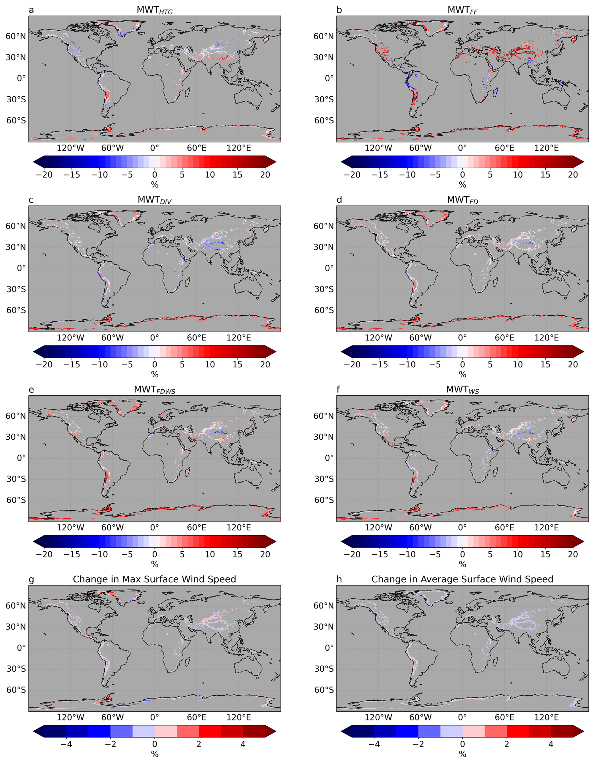
Figure A2 The decade percentage difference in MWT between 11950–1959 and 2040–2049, for the six MWT indices using EC-Earth-3P-HR with grid spacing domain of 36 km, averaged over two ensemble member runs.

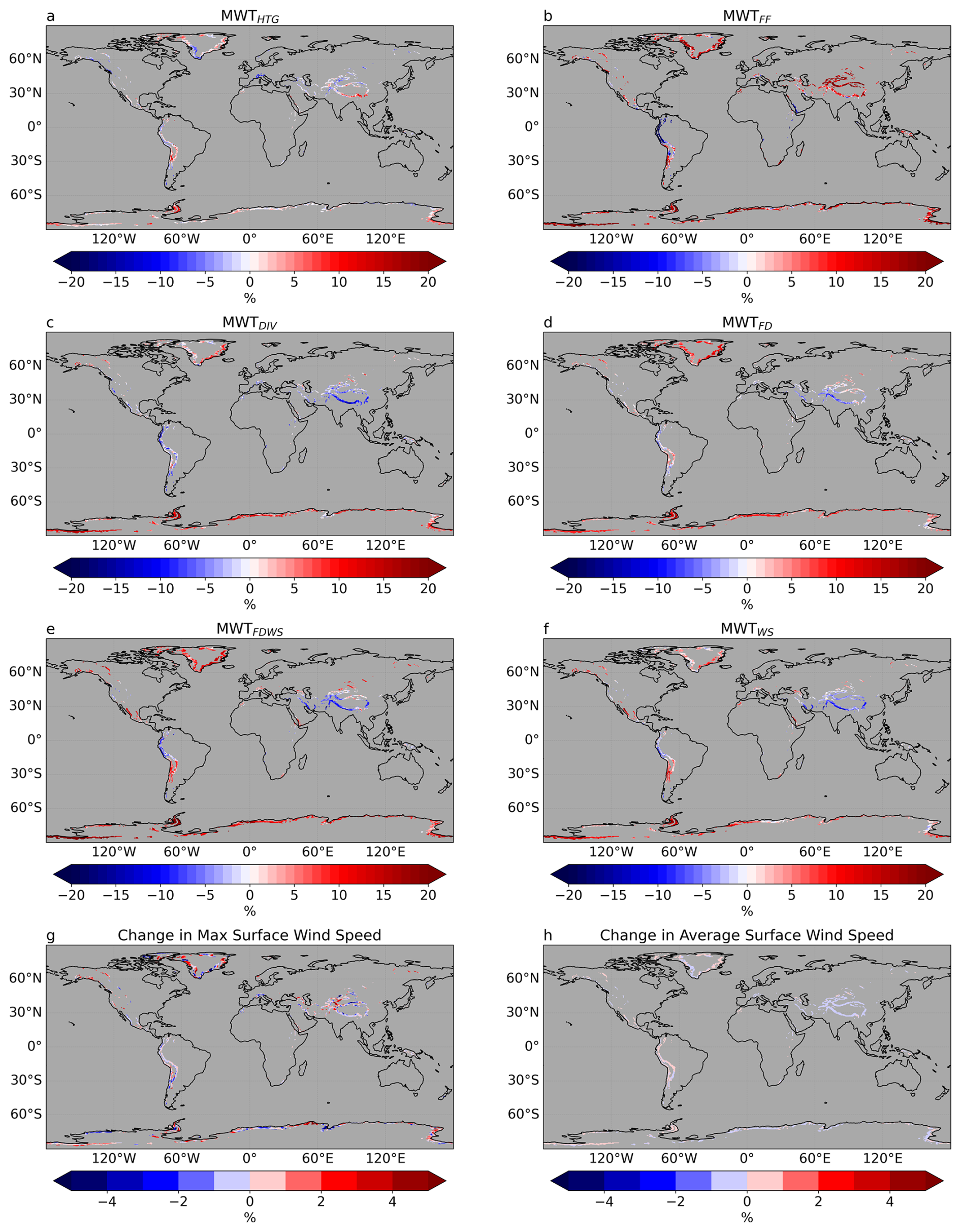
Figure A3 The decade percentage difference in MWT between 1950–1959 and 2040–2049 for the six MWT indices using Max-Planck Institute GCM MPI-ESM1.2-XR with grid spacing domain of 34 km.

Appendix B: Continental index and model variability in seasonal MWT projections for Europe, Africa, Australian Continent and Antarctic

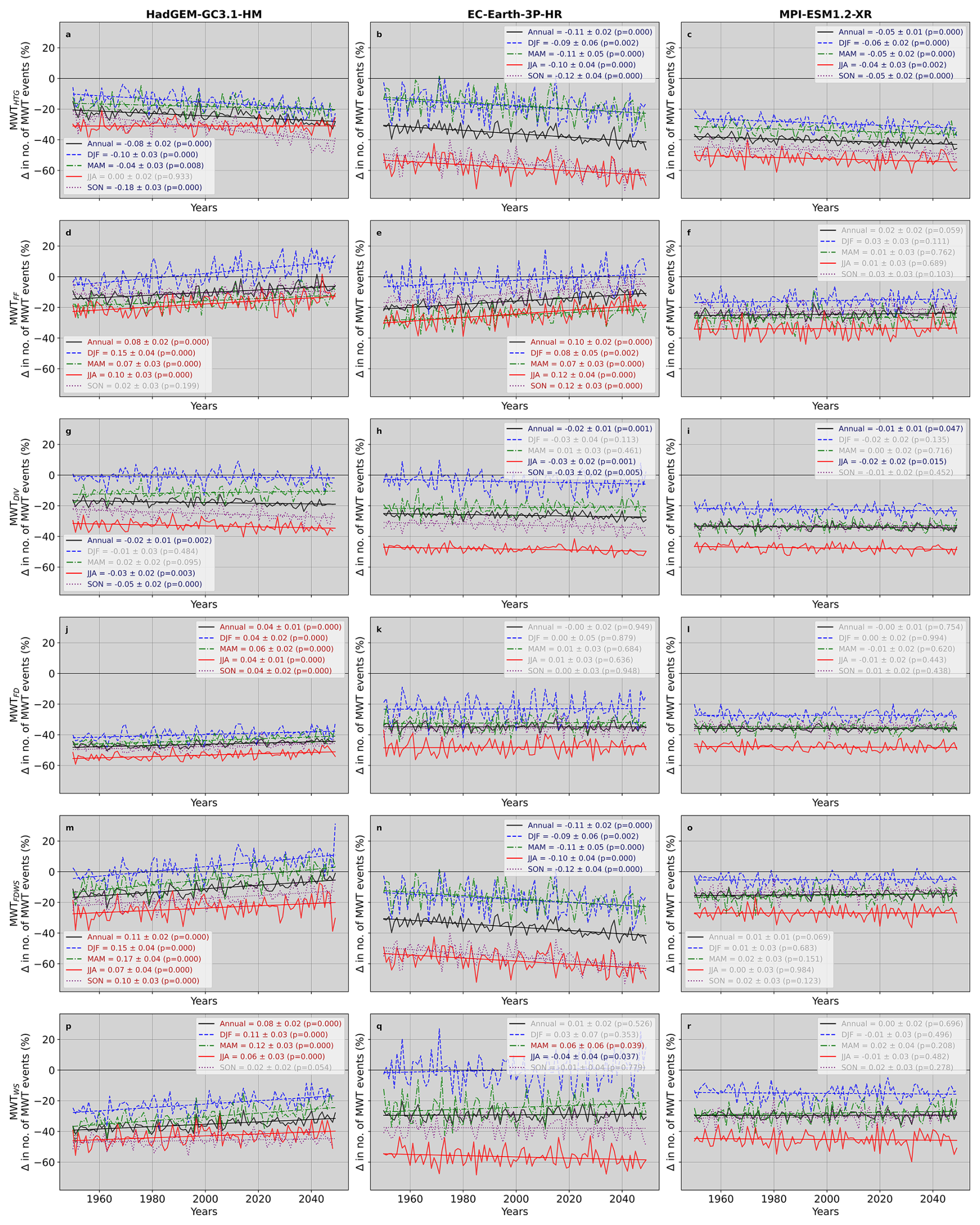
Figure B1 Line plots of relative percentage change over Europe for each year and season compared to a 1950 decadal global references, for each GCM; HadGEM3-GC3.1-HM, EC-Earth-3P-HR, and MPI-ESM1.2-XR and for each index. Line colour and marking differ for each season, with DJF blue and dashed, MAM green and dash dotted, JJA red and soild, SON purple and dotted. Annual change, which includes all seasons is black and solid.

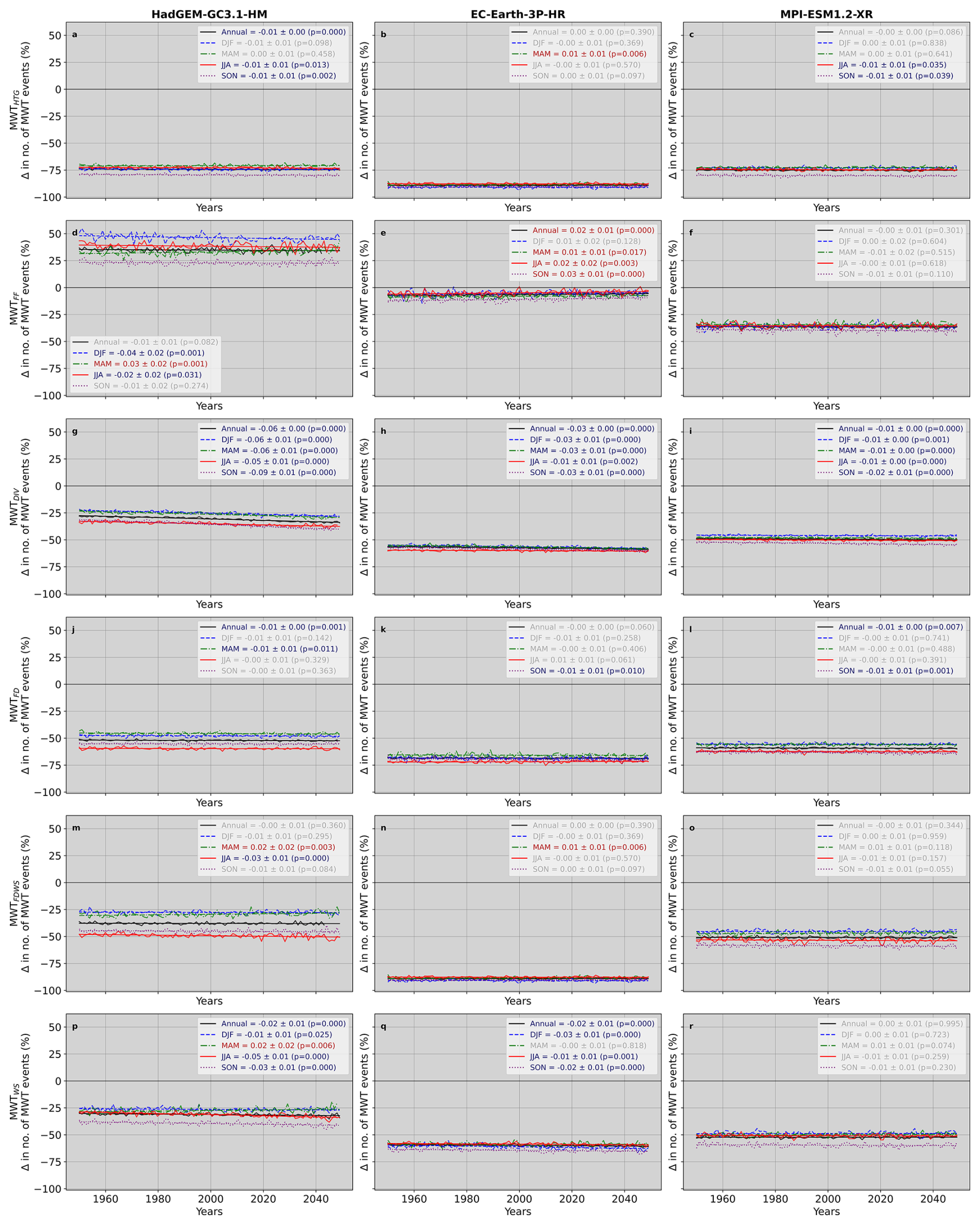
Figure B2 Line plots of relative percentage change over Africa for each year and individual season compared to a 1950 decadal global references, for each GCM; HadGEM3-GC3.1-HM, EC-Earth-3P-HR, and MPI-ESM1.2-XR and for each index. Line colour and marking differ for each season, with DJF blue and dashed, MAM green and dash dotted, JJA red and soild, SON purple and dotted. Annual change, which includes all seasons is black and solid.

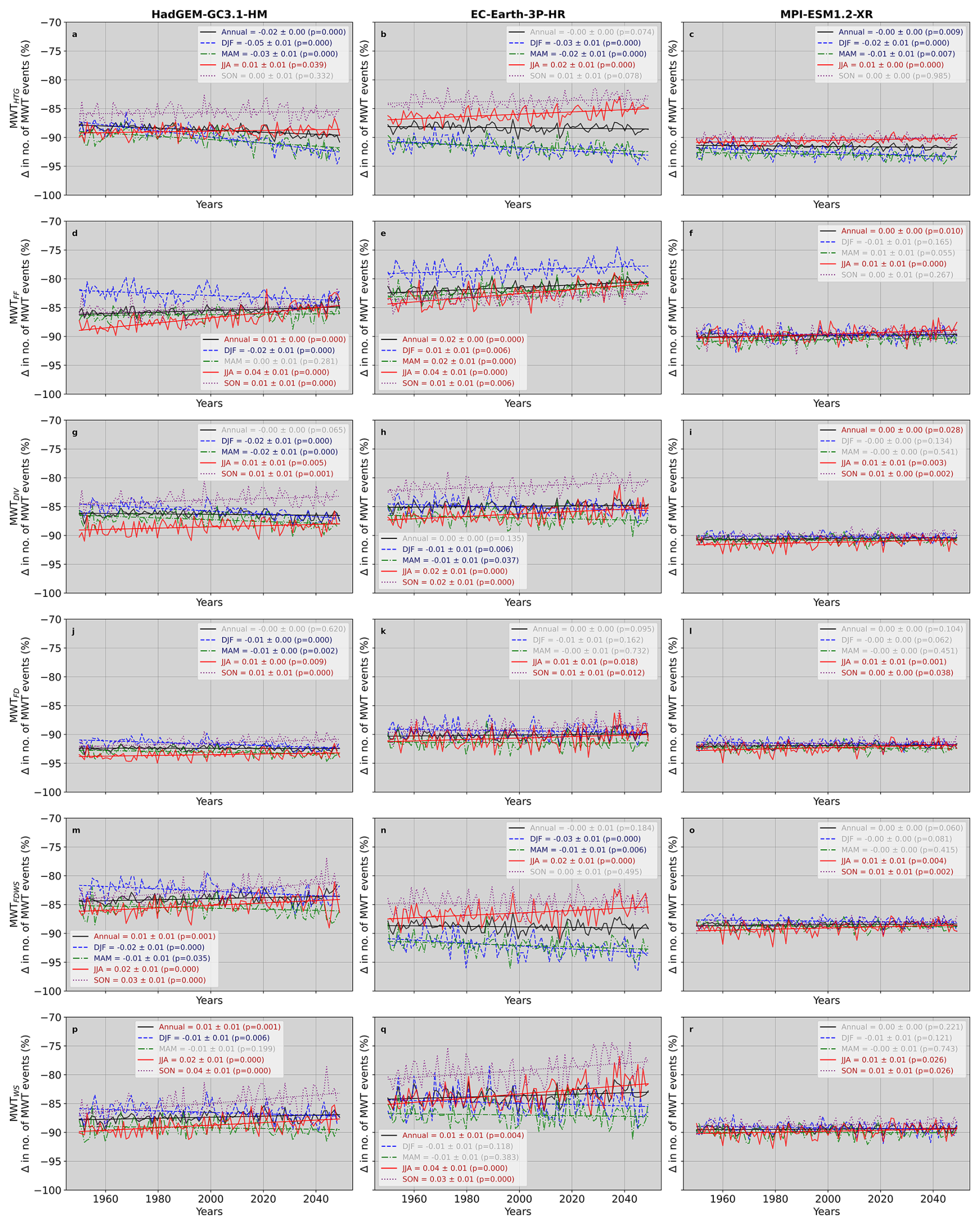
Figure B3 Line plots of relative percentage change over the Australian continent for each year and season compared to a 1950 decadal global references, for each GCM; HadGEM3-GC3.1-HM, EC-Earth-3P-HR, and MPI-ESM1.2-XR and for each individual index. Line colour and marking differ for each season, with DJF blue and dashed, MAM green and dash dotted, JJA red and solid, SON purple and dotted. Annual change, which includes all seasons is black and solid.

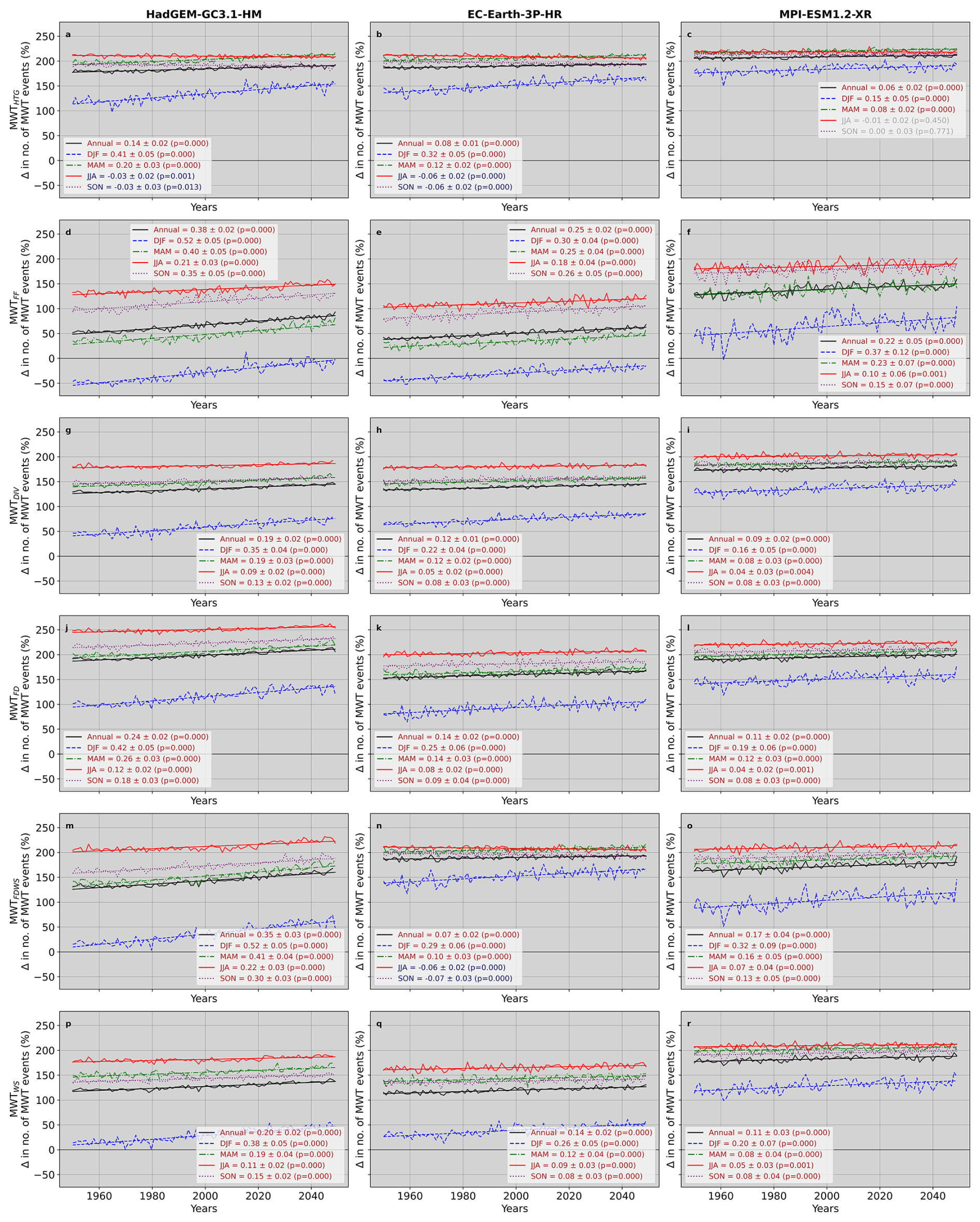
Figure B4 Line plots of relative percentage change over the Antarctic for each year and season compared to a 1950 decadal global references, for each GCM; HadGEM3-GC3.1-HM, EC-Earth-3P-HR, and MPI-ESM1.2-XR and for each individual index. Line colour and marking differ for each season, with DJF blue and dashed, MAM green and dash dotted, JJA red and soild, SON purple and dotted. Annual change, which includes all seasons is black and solid.

Appendix C: Clear air turbulence indices

These are the indices used in combination with our terrain height, gradient and wind speed requirements to calculate mountain wave turbulence. As mentioned in methodology we focus on 200 hPa, note some indices use a vertical component and spread from 250 to 150 hPa. These indices are combined with Ds to create MWT indices (Sect. 2.1).

Wind speed

$$\sqrt{u^{\mathrm{2}}+v^{\mathrm{2}}}$$

Magnitude of horizontal temperature gradient

$$\sqrt{{\left({\displaystyle \frac{\mathrm{d}T}{\mathrm{d}x}}\right)}^{\mathrm{2}}+{\left({\displaystyle \frac{\mathrm{d}T}{\mathrm{d}y}}\right)}^{\mathrm{2}}}$$

Magnitude of horizontal divergence

$$\left|{\displaystyle \frac{\mathrm{d}u}{\mathrm{d}x}}+{\displaystyle \frac{\mathrm{d}v}{\mathrm{d}y}}\right|$$

Flow deformation

$$\sqrt{{\left({\displaystyle \frac{\mathrm{d}v}{\mathrm{d}x}}+{\displaystyle \frac{\mathrm{d}u}{\mathrm{d}y}}\right)}^{\mathrm{2}}+{\left({\displaystyle \frac{\mathrm{d}u}{\mathrm{d}x}}-{\displaystyle \frac{\mathrm{d}v}{\mathrm{d}y}}\right)}^{\mathrm{2}}}$$

Flow deformation times wind speed

$$\sqrt{{\left({\displaystyle \frac{\mathrm{d}v}{\mathrm{d}x}}+{\displaystyle \frac{\mathrm{d}u}{\mathrm{d}y}}\right)}^{\mathrm{2}}+{\left({\displaystyle \frac{\mathrm{d}u}{\mathrm{d}x}}-{\displaystyle \frac{\mathrm{d}v}{\mathrm{d}y}}\right)}^{\mathrm{2}}}\cdot \sqrt{u^{\mathrm{2}}+v^{\mathrm{2}}}$$

Frontogenesis function

$${\displaystyle \frac{\mathrm{d}u}{\mathrm{d}\mathit{\theta }}}\left({\displaystyle \frac{\mathrm{d}v}{\mathrm{d}\mathit{\theta }}}{\displaystyle \frac{\mathrm{d}u}{\mathrm{d}x}}+{\displaystyle \frac{\mathrm{d}v}{\mathrm{d}\mathit{\theta }}}{\displaystyle \frac{\mathrm{d}u}{\mathrm{d}y}}\right)+{\displaystyle \frac{\mathrm{d}v}{\mathrm{d}\mathit{\theta }}}\left({\displaystyle \frac{\mathrm{d}u}{\mathrm{d}\mathit{\theta }}}{\displaystyle \frac{\mathrm{d}v}{\mathrm{d}x}}+{\displaystyle \frac{\mathrm{d}u}{\mathrm{d}\mathit{\theta }}}{\displaystyle \frac{\mathrm{d}v}{\mathrm{d}y}}\right)$$