Spread/error relationship and spatial error representation in precipitation nowcasting: comparison of STEPS and generative AI

The predictability of the generative AI-based nowcasting model LDCast is evaluated over Belgium, together with the pysteps implementation of the nowcasting algorithm STEPS. Neither STEPS nor LDCast were fine-tuned for the Belgian region, so both models are evaluated under conditions in which they will most likely be used in practice at national weather offices. STEPS and LDCast are slightly underdispersive, but the ensemble spread provides an estimation of the error at almost all scales. Both models adapt the properties of their ensembles to the type of event, either convective or stratiform. The spatial scores of the STEPS and LDCast ensembles are compared with those of surrogate ensembles, revealing that both STEPS and LDCast have very little ability to spatially localise the error of the ensemble mean. This suggests that the content of STEPS and LDCast ensembles is informative in terms of statistics, but not in terms of dynamics.

1 Introduction

Many artificial intelligence (AI) models for weather and climate have been developed recently. However, detailed evaluations of these models remain limited and are often done from a statistical point of view, using general scores such as the RMSE between a single forecast (or the ensemble mean) and the observations. In order to be used by forecasters in operational activities, the consistency of the meteorological characteristics of their nowcasts must be assessed (Bouallègue et al., 2024; Radford et al., 2025; Bröcker et al., 2026).

Since the dawn of General Circulation Models (GCMs), there have been many in-depth analyses of their dynamics and predictability in the past 70 years (e.g. Kalnay, 2003; Bauer et al., 2015). Recently, Artificial Intelligence Weather Prediction (AIWP) models such as Pangu-Weather, GraphCast, and FourCastNet were developed, and their forecasts for various events of interest have been compared in detail with those from Numerical Weather Prediction (NWP) models (Olivetti and Messori, 2024; Charlton-Perez et al., 2024; Pasche et al., 2025; Hua et al., 2025). Baño-Medina et al. (2025) also conducted a sensitivity analysis of initial conditions on the Spherical Fourier Neural Operator (SFNO) in a storm environment, finding properties similar to an NWP model.

Methods for estimating uncertainties in AI model forecasts are still under development. Bred vectors for AIWP models were constructed by Baño-Medina et al. (2025), Mahesh et al. (2025) and Almeida et al. (2026), and a similar method was developed by Pu et al. (2025). On the other hand, the uncertainty could also be represented naturally by generative models as illustrated in Lang et al. (2026). These models produce nondeterministic forecasts, which makes it easy to create ensembles. Generative models such as DGMR (Ravuri et al., 2021) and LDCast (Leinonen et al., 2023) can also be trained to produce realistic forecasts that retain sharpness instead of being smoothed out due to the loss of predictability with increasing lead time.

However, the relevance of ensemble properties of generative models for operational activities has not been sufficiently investigated. Indeed, these model ensembles are primarily evaluated over the whole dataset using global scores (Lang et al., 2026) or global rank histograms (Price et al., 2023; Leinonen et al., 2023). Some models are also evaluated on a few selected events through a meteorologist's comparison and ranking of the outputs of different models (Ravuri et al., 2021; Zhang et al., 2023).

These evaluation methods are necessary first steps, but a deeper understanding of the characteristics of generative models is needed. This includes their dynamical properties, as well as their particular behavior and biases for different weather types or spatial scales. The central question of this paper is therefore to characterize the information contained in the ensembles generated by a generative nowcasting model, with a focus on the error representation in the ensembles (both in size and in localization).

This work aims to provide this characterization for LDCast (Leinonen et al., 2023), a generative model for rainfall nowcasting. It is evaluated using the Belgian radar composite RADCLIM (Goudenhoofdt and Delobbe, 2016; Journée et al., 2023), but it has not been retrained on this dataset. Therefore, the model weights are the original ones, and the model can be considered pre-trained for rainfall nowcasting. The pysteps implementation of the nowcasting algorithm STEPS (Bowler et al., 2006; Seed et al., 2013; Pulkkinen et al., 2019) is evaluated in parallel to clarify which approach is best in producing rainfall forecasts for both convective and stratiform rainfall cases.

2 Data and methods

2.1 Data and preprocessing

The radar product on which STEPS and LDCast are evaluated in this work is RADCLIM (Goudenhoofdt and Delobbe, 2016; Journée et al., 2023): it is a quantitative precipitation estimation product based on radar measurements, which are merged with rain gauge measures. Several techniques exist for this merging: the product used in this study was obtained with the Kriging with External Drift (KED) technique. The time resolution is 5 min and the spatial resolution is 1 km × 1 km. The evaluation domain is a 320 px × 320 px square in the radar frame.

Ten stratiform and ten convective events were selected based on the convective precipitation and the mean large-scale precipitation derived from ERA5 (Hersbach et al., 2023). Events are considered convective if their mean convective precipitation was greater than 10⁻⁴ mm h⁻¹ and their large-scale precipitation was less than 10⁻⁶ mm h⁻¹. Similarly, stratiform events were selected as those with a mean convective precipitation below 10⁻⁷ mm h⁻¹ and a large-scale precipitation above 8.07 × 10⁻⁴ mm h⁻¹.

As both STEPS and LDCast transform the rain rate to a logarithmic scale, all computations in this work are done with a similar scale. The transformation used in this work is

$$\begin{array}{}\text{(1)}& f\left(R\right)=\left\{\begin{array}{cc}\mathrm{10}{\log }_{\mathrm{10}}\left(R\right)& \text{for}R\ge \mathrm{0.1}\mathrm{mm}{\mathrm{h}}^{-\mathrm{1}}\\ -\mathrm{15}& \text{for}R<\mathrm{0.1}\mathrm{mm}{\mathrm{h}}^{-\mathrm{1}}\end{array}\right.\end{array}$$

The unit after this transformation is dBR.

2.2 Models

The two nowcasting models considered in this work are STEPS and LDCast. STEPS is built on Lagrangian persistence (Zawadzki et al., 1994), which consists in advecting the rainfall field with a motion field estimated through an optical flow algorithm. In STEPS, the rainfall field is in addition decomposed into fields of different spatial scales via a cascade, and each of the levels of the cascade evolves according to an auto-regressive (AR) process, usually of order 2. There are two sources of perturbation in STEPS: the motion field is stochastically perturbed via the method designed in Bowler et al. (2006) (named BPS in the pysteps library; Pulkkinen et al., 2019), and the field intensities are perturbed via the noise component of the AR(2) processes (Bowler et al., 2006). The noise itself was originally generated with a parametric method, but the nonparametric method developed in Seed et al. (2013) is now more commonly used. STEPS is implemented at the Royal Meteorological Institute of Belgium (RMI) with pysteps (Pulkkinen et al., 2019).

In STEPS, there is no value for the pixels for which the value should come from the advection of pixel values out of the radar frame. To avoid as much as possible this problem, STEPS nowcasts were produced using the whole available radar domain of RADCLIM (see Sect. 2.1), and the analysis presented in this work was performed on a smaller 320 px × 320 px square extracted from this domain. There were still some pixels with missing values after doing this, and these were assigned the no-rain value of −15 dBR. In stratiform STEPS ensembles, the fraction of those pixels in an ensemble at a given lead time is at most 3 % and it is smaller than 1 % for convective STEPS ensembles. The effects of such missing values in STEPS nowcasts are therefore supposed to be negligible.

LDCast is a latent diffusion model, meaning that a sequence of rainfall fields is first encoded to a latent space learned by the variational autoencoder of the model. The forecaster network then predicts the latent representation of future rainfall fields. Conditionally to this output, the denoiser stack produces different members, which are finally transformed back from the latent space to rainfall fields (Leinonen et al., 2023).

LDCast was trained on the radar product with code RZC, which uses only data from the radar themselves, while the RADCLIM dataset used in this work includes a merging with rain gauges. Merging with rain gauges is known to smooth out small scales (Ochoa-Rodriguez et al., 2019), so that a difference between the nowcasts of LDCast and the radar observations at small scales can be expected.

The LDCast nowcasts were first produced on a 416 px × 416 px area extracted from the radar domain. The nowcasts were then cropped to the 320 px × 320 px square used to evaluate the models.

3 Results

Ensembles of nowcasts were produced with STEPS and with LDCast for the selected events (Sect. 2.1), in order to analyze their behavior in dynamically different situations. The members of the ensembles are denoted $\mathit{\{}{\mathit{x}}_i{\mathit{\}}}_{i=\mathrm{1},\mathrm{\dots },N}$ with N = 50. The time dependence is omitted in the notation for simplicity.

The ensemble mean is computed pixel-wise as

$$\begin{array}{}\text{(2)}& \stackrel{\mathrm{‾}}{\mathit{x}}={\displaystyle \frac{\mathrm{1}}{N}}\sum _{i=\mathrm{1}}^N{\mathit{x}}_i.\end{array}$$

The observations (radar images) are denoted by y, and the pixel-wise error is

$$\begin{array}{}\text{(3)}& \mathit{e}=\mathit{y}-\stackrel{\mathrm{‾}}{\mathit{x}}.\end{array}$$

The residual vectors v_i of the members with respect to the mean are defined as

$$\begin{array}{}\text{(4)}& {\mathit{v}}_i={\mathit{x}}_i-\stackrel{\mathrm{‾}}{\mathit{x}}.\end{array}$$

The power spectrum of a field x, at a scale $\mathrm{1}/k$, is

$$\begin{array}{}\text{(5)}& \text{PS}(\mathit{x}{)}_k=\langle |X_{\mathit{k}}{|}^{\mathrm{2}}{\rangle }_{\left|\mathit{k}\right|=k},\end{array}$$

where X_k is the Fourier coefficient of x at wavevector k and $\langle \cdot {\rangle }_{\left|\mathit{k}\right|=k}$ denotes the average over the wavevectors with norm equal to k.

The analysis of the ensembles of nowcasts is presented below. Examples of nowcasts produced with STEPS and LDCast, as well as well a spatial representation of the mean error and of the spatial standard deviation in the ensembles, are provided in the Supplement (Figs. S1, S2, S3 and S4).

3.1 Spectral error and spectral variance

The spectral error is computed as the power spectrum of the pixel-wise error e. It is a scale-by-scale decomposition of the mean squared error of the ensemble mean. On the other hand, the spectral variance is defined as

$$\begin{array}{}\text{(6)}& {\mathit{\sigma }}_k^{\mathrm{2}}={\displaystyle \frac{\mathrm{1}}{N-\mathrm{1}}}\sum _{i=\mathrm{1}}^N\text{PS}{\left({\mathit{x}}_i-\stackrel{\mathrm{‾}}{\mathit{x}}\right)}_k\end{array}$$

and is often called the spread in meteorological applications.

The spectral error and spectral variance for STEPS and for LDCast, together with the power spectra of observations, are displayed in Fig. 1 (average over the selected events). The color of the curves represents the lead time at which the spread and the error are computed.

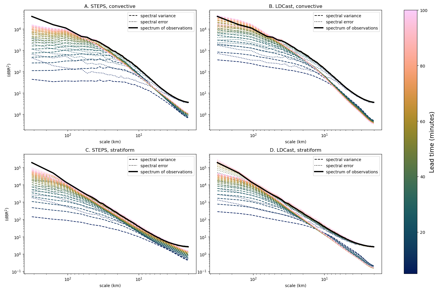
Figure 1 Spectral error and spectral variance, for STEPS and for LDCast, and for convective and for stratiform events (averaged over events). Dashed lines display the spectral variance and dotted lines display the spectral error. The color represents the lead time. The power spectra of observations are represented by thick black lines.

Both the spectral error and the spectral variance increase with lead time and eventually saturate to the power spectrum of the observation (see Appendix B). The error at some scales is immediately saturated (Pulkkinen et al., 2019): depending on the model and on the event type, the largest saturated scale after 5 min is between 5 and 10 km.

For a well-calibrated ensemble, the error and the spread should be equal, provided the ensemble mean is not biased (Fortin et al., 2014). Whether STEPS and LDCast ensembles are well-calibrated is assessed more precisely with Fig. 2, where the scale-by-scale ratio of the spectral variance over the de-biased spectral error is displayed. A ratio smaller than 1 indicates underdispersion, while there is overdispersion when it is larger than 1. The spread $/$ error ratio in Fig. 2 was computed with the de-biased error, meaning that a small bias of the ensemble mean was removed in Eq. (3).

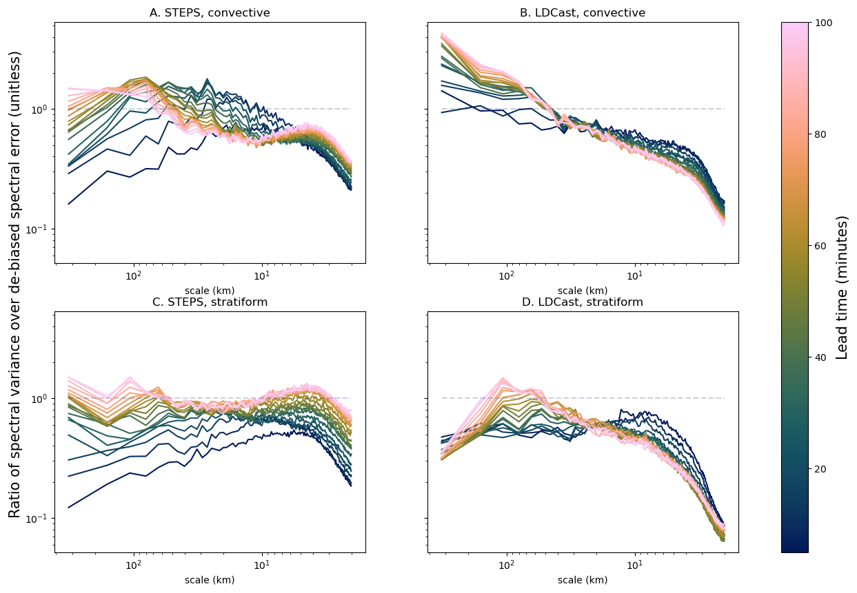
Figure 2 Ratios of the spectral variance over the de-biased spectral error, for STEPS and LDCast, and for convective and stratiform events (averaged over the events). The color represents the lead time. Horizontal dashed grey lines mark where the ratio is 1. Ratio < 1: underdispersion, ratio > 1: overdispersion.

Overall, both models have variance $/$ error ratios close to 1 for scales above 5 km. LDCast is slightly underdispersive, except for the larger scales in convective events, where it is rather overdispersive. On the other hand, for stratiform events, STEPS ensembles are underdispersive for short lead times but become well calibrated for longer lead times. In convective cases, STEPS is either underdispersive or overdispersive depending on the lead time and the scale.

The spectral error and the power spectrum of observations flatten out for scales smaller than 5 km. This is however not the case for the spectral variance of STEPS and LDCast, so that the ensembles seem to be underdispersed. However, the power spectrum of radar images is known to flatten due to white noise contamination at these scales due to non-meteorological sources (Seed et al., 2013). Merging with rain gauge, as is done for the radar data used in this work, is also known to smooth the small scales (Ochoa-Rodriguez et al., 2019), and that explains the shape of the corresponding part of the spectral error. Therefore, the flattening of the power spectrum of radar images can be considered as not physical, and this underdispersion should not be identified as a weakness of the ensembles. This occurs at scales for which the error is immediately saturated, so that this is anyway irrelevant from a forecasting point of view.

It is not clear why the spectral variance of STEPS is not as large as the spectral error, since STEPS mainly extrapolates radar observations. On the other hand, LDCast was trained on a radar product without rain gauge merging, so that it can be expected that its nowcasts behave differently at small scales than the radar observations used in this work.

3.2 Morphology of STEPS and LDCast ensembles

The ensemble covariance matrix and its eigenvalues and eigenvectors are used in this section to investigate the morphology of the ensembles. If the ensemble is considered as a cloud of points in phase space, the eigenvectors of the covariance matrix point in the directions in which the ensemble is the most extended (as measured by the variance in these directions, which are given by the associated eigenvalues). The method is therefore equivalent to Principal Component Analysis where all components are kept. This tool was originally introduced by Patil et al. (2001) and then by Oczkowski et al. (2005) to estimate the dimension of ensemble of forecasts (“E dimension”), reducing the information in the covariance matrix to one number. Other works (Satterfield and Szunyogh, 2011; Ono, 2025) followed in that direction. On the other hand, the full eigenvalue spectrum of the covariance of ensemble members was used by Snyder et al. (2003) in an idealized model.

Some of the authors who developed the “E dimension” have also later used the information in the eigenvectors of the ensemble covariance matrix, by using the fraction of error explained by the eigenvectors as a metric to evaluate ensembles of forecasts (Szunyogh et al., 2005; Satterfield and Szunyogh, 2010).

The covariance matrix is largely singular since the ensemble members have 320² = 102 400 components, while the ensembles have only 50 members. Actually, the covariance matrix has only 49 non-zero eigenvalues because it is constructed out of the residual vectors v_i, which satisfy ∑_iv_i = 0 (and it was supposed that this is the only relationship between them). The eigenvalues of the covariance matrix are denoted λ_i, and the eigenvectors u_i are also called perturbation modes (PM). Example of eigenvectors of covariance matrices are shown in the Supplement (Figs. S5 to S12).

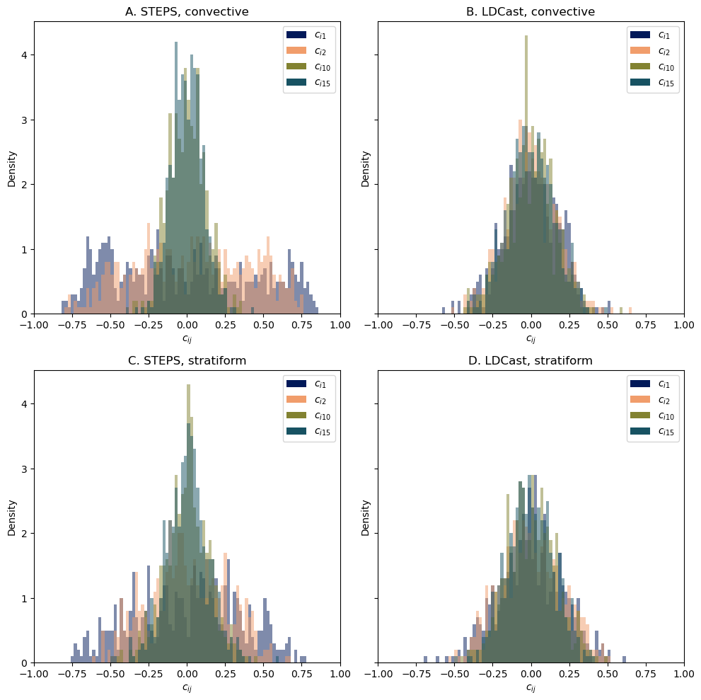
Panels (A) and (B) of Fig. 3 display the eigenvalues λ_i of the covariance matrix for both models, averaged over events. A few eigenvalues largely dominate the others, especially in convective STEPS ensembles (panel A). To investigate the geometry of these ensembles, the residual vectors v_i of the members with respect to the ensemble mean were considered (see Eq. 4). There are roughly speaking two different geometries that could explain this: (a) the v_i have comparable norms but they align along the directions of the first eigenvectors of the covariance matrix or (b) the v_i are each pointing in different directions but some of them have much larger norms. In order to determine which of the two geometries is actually realized in this case, the cosine c_ij of the angle between the residual vector v_i and u_j was computed for all i and j. It is computed as

$$\begin{array}{}\text{(7)}& c_{ij}={\displaystyle \frac{{\mathit{v}}_i\cdot {\mathit{u}}_j}{\left|{\mathit{v}}_i\right|}}\end{array}$$

since the eigenvector u_j has a unit norm.

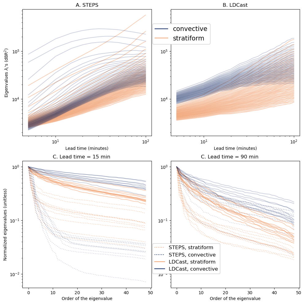
Figure 3 Eigenvalues λ_i of the covariance matrix. Evolution of the eigenvalues for convective and stratiform events for STEPS (A) and LDCast (B). Normalized eigenvalues for convective and stratiform events, for STEPS and LDCast, after 15 min (C) and after 90 min (D) (each line is the eigenvalue spectrum for one event).

Figure 4 represents the histograms of values of c_ij for $j=\mathrm{1},\mathrm{2},\mathrm{10}$ and 15, for a lead time of 15 min. In convective STEPS ensembles (panel A), the distributions of c_i1 and c_i2 contain much higher values than the distributions of c_i10 and c_i15, meaning that the v_i project much more on the first and the second eigenvectors than on the 10th and the 15th. This is also the case for stratiform STEPS ensemble, albeit to a lesser extent. The conclusion is that the v_i in these ensembles align along the first eigenvectors (option a).

Figure 4 Histograms of the c_ij for $j=\mathrm{1},\mathrm{5},\mathrm{10}$ and 15 (for all events) after 15 min.

The evolution of eigenvalues λ_i of the covariance matrix for stratiform events is comparable for STEPS and LDCast: the eigenvalues increase steadily following power laws of the lead time (Fig. 3, panels A and B). This is also the case for convective LDCast ensembles. These power laws should be connected with the theoretical time that an error, initially located at small scales, needs to reach a given larger scale. Indeed, the fact that the error grows as power law of the time is consistent with the limited predictability at the nowcasting scales. This limited predictability is related to the structure of the energy spectrum of atmospheric fields at these scales, following closely a $-\mathrm{5}/\mathrm{3}$ power law (Rotunno and Snyder, 2008).

Panels (C) and (D) of Fig. 3 show, for two different lead times, the spectrum of the normalized eigenvalues. These are the eigenvalues divided by the highest one in the ensemble at that lead time, and they allow to better understand the relative sizes of the perturbation modes. Consistent with the panels (A) and (B), it appears that LDCast ensembles have generally more homogeneous eigenvalue spectra (i.e. have more eigenvalues of similar size) than STEPS ensembles. Convective LDCast ensembles exhibit more homogeneous eigenvalue spectra than stratiform LDCast ensembles, especially at long lead times. As already noted from panel (A), it is also obvious that STEPS ensembles are largely dominated by a few eigenvalues: convective STEPS ensembles are dominated by ∼ 10 eigenvalues, while stratiform STEPS ensembles are dominated by ∼ 5 eigenvalues. However, the relative size of higher-order eigenvalues (order > 5 in stratiform ensembles, order > 10 in convective ensembles) is larger in stratiform STEPS ensembles than in convective STEPS ensembles.

The power spectra of the eigenvectors of the covariance matrix are displayed in Fig. 5, for different lead times, for stratiform and convective events. The color represents the associated eigenvalues λ_i. Overall, the perturbation modes gradually develop over larger scales, while the spectrum profile remains the same for small scales. This shows that the directions of perturbation evolve in phase space with the lead time: at long lead times, the perturbations are vectors pointing in directions corresponding to larger scales than at the beginning of the nowcast.

It also appears that eigenvectors with higher eigenvalues have more power at large scales. This leads to a hierarchy: perturbations with larger amplitudes affect the large scales more. This is in agreement with the fact that, for a given scale, there is a maximum size for the error (see Fig. 1), so that once a perturbation reaches the saturation value at a given scale, it propagates to larger scales.

For both STEPS and LDCast, the eigenvectors of stratiform ensembles (especially the eigenvectors associated with the highest eigenvalues) have more power at larger scales than those of convective ensembles. This means that the perturbations contained in stratiform ensembles are at larger scales than those in convective ensembles.

The curves standing out in the top row (A) of Fig. 5 for short and intermediate lead times are those of the power spectra of the eigenvectors that largely dominate the STEPS ensembles in convective cases (panel A of Fig. 3). Similar power spectra are also present in stratiform STEPS ensembles.

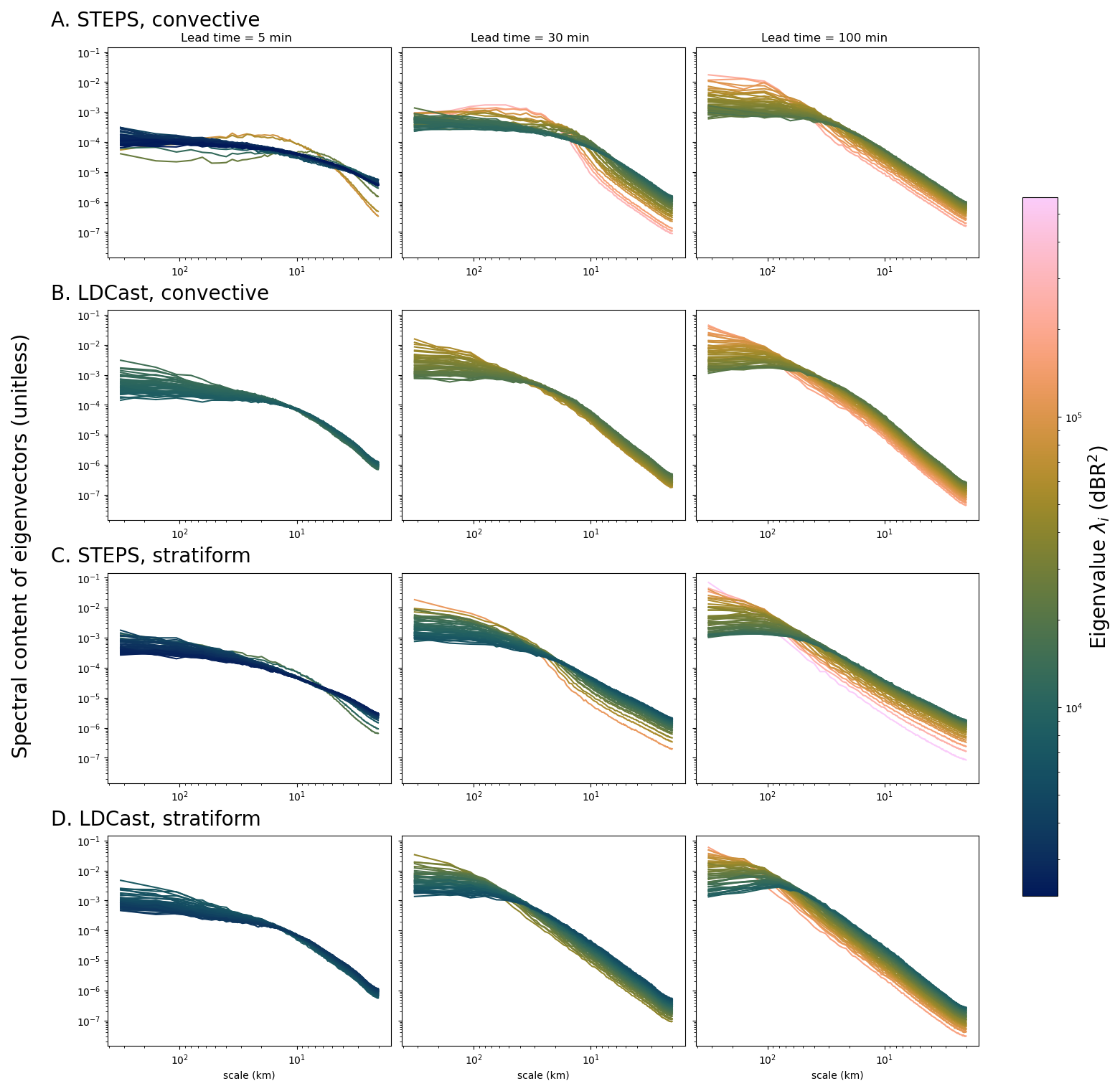
Figure 5 Evolution of the spectra of the eigenvectors for convective and stratiform events, for LDCast and STEPS ensembles. The spectra are averaged over all events. The color represents the corresponding eigenvalue.

Note that the eigenvectors have unit norm so that values in a power spectrum are only meaningful relative to other values in that power spectrum. For example, the spectra of LDCast eigenvectors at small scales seem to decrease with lead time, but this is not due to an absolute decrease in the small-scale variability. It is rather due to a decrease in the small-scale variability relative to the large-scale variability in the same vectors.

3.3 Spatial skill of STEPS and LDCast ensembles

This section presents results assessing the skill of ensemble members to spatially represent the error. The focus is particularly on evaluating whether the ensembles contain any spatial information beyond that present in the ensemble mean.

Two metrics are considered. The first is the Perturbation versus Error Correlation Analysis (PECA) score (Wei and Toth, 2003), which is called cos γ(e,p) here in order to emphasize its geometric interpretation in phase space. Indeed, it is the cosine of the angle between the error e and its projection p on the subspace spanned by the residual vectors v_i. Using the fact that the eigenvectors of the covariance matrix are orthonormal and span the same subspace as the v_i, p can be written as

$$\begin{array}{}\text{(8)}& \mathit{p}=\sum _i({\mathit{u}}_i\cdot \mathit{e}){\mathit{u}}_i\end{array}$$

and its norm is $\left|\mathit{p}\right|$ = $\sqrt{{\sum }_i({\mathit{u}}_i\cdot \mathit{e}{)}^{\mathrm{2}}}$. So cos γ(e,p) can be computed in terms of the scalar product between e and p as

$$\begin{array}{}\text{(9)}& \cos \mathit{\gamma }(\mathit{e},\mathit{p})={\displaystyle \frac{\mathit{e}\cdot \mathit{p}}{\left|\mathit{e}\right|\left|\mathit{p}\right|}},\end{array}$$

or in terms of the ratio between the norm of p and the norm of e:

$$\begin{array}{}\text{(10)}& \cos \mathit{\gamma }(\mathit{e},\mathit{p})={\displaystyle \frac{\left|\mathit{p}\right|}{\left|\mathit{e}\right|}}\end{array}$$

since e⋅p = ${\sum }_i({\mathit{u}}_i\cdot \mathit{e}{)}^{\mathrm{2}}$ = $|\mathit{p}{|}^{\mathrm{2}}$. These expressions show that cos γ(e,p) indicates the extent to which the error is captured by the ensemble members.

This metric is indeed equal to the PECA score, except that the error and the perturbations are computed with respect to a control run for the PECA score. Apart from that, minimizing the L₂-norm of $\mathit{e}-{\sum }_i{\mathit{\alpha }}_i{\mathit{v}}_i$ amounts to constructing the projection of e on the space spanned by the v_i.

The same quantity was also introduced independently by Szunyogh et al. (2005) and Satterfield and Szunyogh (2010) as the Explained Variance (EV) to evaluate the efficiency of data assimilation schemes to provide initial conditions leading, under the perfect model hypothesis, to ensembles of forecasts capturing the error. Finally, Uboldi and Trevisan (2015) also considered that metric to estimate the ability of breeding vectors of a realistic model to capture the error growth in a convective situation.

The second metric considered is the Fraction Skill Score (FSS), which was introduced by Roberts and Lean (2008) as a metric for the spatial accuracy of a deterministic forecast. With respect to the mean square error, it mitigates displacement errors by comparing the forecast and the observation over neighborhoods of different scales. Necker et al. (2024) recently compared different versions of the FSS for ensemble verification, and recommended the “probabilistic FSS” proposed in Schwartz et al. (2010), which is the one used in the current work.

The two metrics are computed for STEPS and LDCast ensembles and compared to those of three types of surrogate ensembles. Surrogate ensembles are generated as follows:

• HIST ensembles: for each member x_i in the original ensemble, a HIST surrogate z_i is generated by shuffling all the pixel values of x_i (x_i and z_i have thus the same histogram of values);

• SPEC ensembles: for each x_i (that we decompose as $\stackrel{\mathrm{‾}}{\mathit{x}}+{\mathit{v}}_i$), a SPEC surrogate is generated as $\stackrel{\mathrm{‾}}{\mathit{x}}+{\mathit{w}}_i$, where w_i has the same power spectrum as v_i but with random Fourier phases (SPEC surrogates do not have the same histogram of values as the original members);

• MAAFT ensembles: for each x_i, a MAAFT surrogate is built in such a way that it has the same histogram of pixel values as x_i and the same power spectrum for its residual vector as v_i. The name stands for Modified Amplitude Adjusted Fourier Transform.

MAAFT surrogates are inspired from the Iterated Amplitude-Adjusted Fourier Transform (IAAFT) of Schreiber and Schmitz (1996). The construction of SPEC and MAAFT ensembles is detailed in Appendix A.

3.3.1 Using cos γ(e,p)

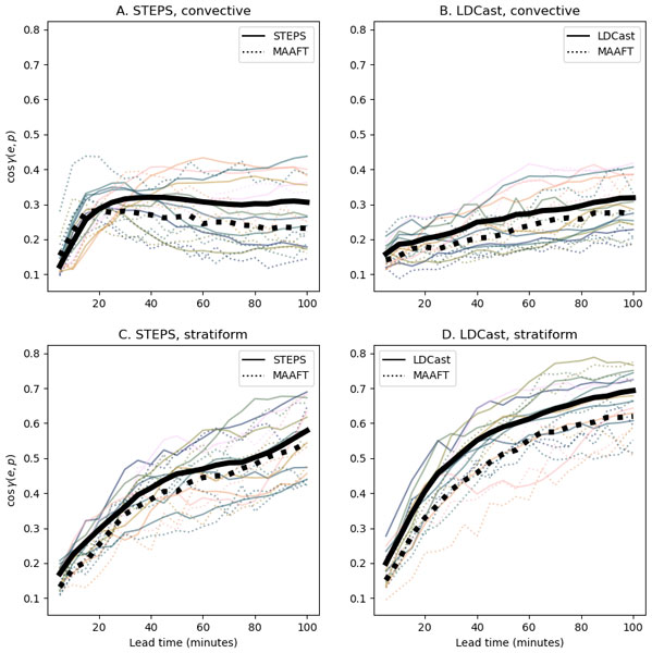
The cosine of the angle between the error e and its projection p on the STEPS and LDCast residual vectors v_i is represented by solid lines in the panels of Fig. 6. The thin lines depict this cosine for each event, and the thick line shows the mean of this quantity over the events. The dotted lines represent the same quantity for the MAAFT ensembles constructed from the original STEPS and LDCast ensembles.

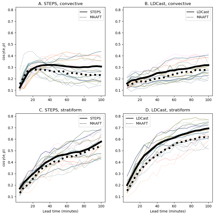
Figure 6 Comparison of cos γ(e,p) of the error and its projection on STEPS/LDCast ensembles (solid lines) with the cos γ(e,p) for the corresponding MAAFT ensembles (dotted lines), for all lead times. Thin lines depict cos γ(e,p) for each event and thick lines represent the event average. The MAAFT ensembles whose scores are presented in panels (A) and (C) are built from the corresponding STEPS ensembles, while those whose scores are presented in panels (B) and (D) are built from the corresponding LDCast ensembles.

The cos γ(e,p) values of the surrogate MAAFT ensembles are very close to those of the corresponding STEPS and LDCast ensembles. The reason for this is the shape of the Fourier spectra of the perturbations. Indeed, it was verified that SPEC ensembles (surrogates generated without the constraint on the distribution of values, only imposing the power spectra of residual vectors, see Sect. A) lead to similar values for cos γ(e,p) (Fig. S13). In particular, the spatial localization of the perturbations contained in the v_i of STEPS and LDCast ensembles does not explain the values of cos γ(e,p) of the error with these ensembles, since the same values are reached for surrogate ensembles with random residual vectors where no constraint is imposed on the spatial localization.

One way to understand this is by expressing cos γ(e,p) in terms of Fourier modes: if E_k and V_k are respectively the Fourier coefficients of e and of a residual vector v (of a STEPS, LDCast or MAAFT ensemble) and ${\mathit{\varphi }}_{\mathit{k}}^e$ and ${\mathit{\varphi }}_{\mathit{k}}^v$ the complex phases of these coefficients, the terms in the projection of e on the v_i is proportional to the scalar product of e and v, which is of the form $\left|E_{\mathit{k}}\right|\left|V_{\mathit{k}}\right|\left({\mathit{\varphi }}_{\mathit{k}}^e{\mathit{\varphi }}_{\mathit{k}}^{v*}+{\mathit{\varphi }}_{\mathit{k}}^{e*}{\mathit{\varphi }}_{\mathit{k}}^v\right)$. The moduli $\left|V_{\mathit{k}}\right|$ are imposed when constructing MAAFT ensembles and the complex phases ${\mathit{\varphi }}_{\mathit{k}}^v$ are precisely random. The fact that the values of cos γ(e,p) for a STEPS or an LDCast ensemble are the same as with the corresponding MAAFT ensemble shows that the complex phases ${\mathit{\varphi }}_{\mathit{k}}^v$ are also random for STEPS and LDCast ensembles. Since the spatial localization of the structures of a field is contained in the complex phases of its Fourier coefficients, the fact that the complex phases for the Fourier coefficients of the v_i are random indeed means that the localization of the structures they contain is random.

The value of cos γ(e,p) increases with the lead time and this can be explained by the evolution of the power spectra of the vectors v_i. When the lead time increases, these vectors progressively represent larger perturbations. Because of this, it can be expected that it becomes easier for ensembles to cover the whole domain with independent perturbations of a given scale, and thus to spatially capture the actual instability.

Interestingly, Feng et al. (2024) argued that the error at convective scales always has a negligible projection onto the perturbation modes of an ensemble. While this is always the case at short lead times in Fig. 6, the projection is largely non-negligible for intermediate and long lead times, especially for stratiform events. However, this is because the perturbation modes develop large-scale components that eventually cover the entire domain.

3.3.2 Using the FSS

Figure 7 depicts the FSS averaged over events, for STEPS/LDCast ensembles and for the corresponding MAAFT ensembles, by solid and dotted lines, respectively. The thick black lines (HIST lines) in this figure represent the FSS of the surrogate HIST ensemble (surrogates constructed by simply shuffling the pixel values, without power-spectrum adjustment, see Sect. A). This score remains relatively constant over time, so that only the time average is represented in Fig. 7. This FSS is the one of a random prediction given the distribution of values in the nowcast. For the smallest scales, this FSS is analogous to the random FSS in Roberts and Lean (2008). For the largest scale, it corresponds to their Asymptotic Fraction Skill Score (AFSS) (Roberts and Lean, 2008).

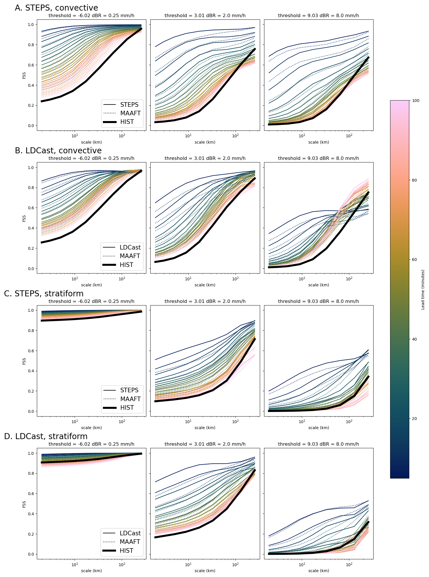
Figure 7 Fraction Skill Scores (FSSs) as functions of scale for (a) convective events and (b) stratiform events, with the time dependence represented by the color. The thin solid lines represent the LDCast FSSs, the dotted lines represent the MAAFT FSSs while the thick solid line represents the HIST FSSs (no time dependence shown). The x axis represents the scale for which the FSS was computed, and is reversed with respect to the previous figures.

The LDCast and the corresponding MAAFT scores saturate with lead time to a value close to the HIST value. Interestingly, the LDCast and STEPS values of the FSS saturate more slowly than the spectral variance in Fig. 1: even at the smallest scales, the FSS saturates after 40 min, whereas the spectral variance is immediately saturated at those scales. The other intriguing feature in this figure is the behavior of LDCast for the highest threshold: for the highest scales for which it is computed, the FSS scores increase with lead time. At the highest scale, the FSS score merely assesses whether there is a correct number (over the whole radar frame) of values above the chosen threshold. In this case, the number of high-intensity values is better estimated as the lead time increases.

The MAAFT FSSs are quite close to STEPS and LDCast FSSs, showing again that the FSS scores of STEPS and LDCast ensembles are mainly due to their statistical properties, but not to the spatial localization of the perturbations in the ensembles.

4 Conclusions

This work investigates the spectral and spatial properties of STEPS ensembles and a pre-trained version of LDCast. In particular, it shows that LDCast and STEPS residual vectors v_i have appropriate sizes with respect to the error since the spread/skill relationships are close to 1. But the directions of v_i in phase space (and thus their localizations in real space) are random, as measured by cos γ and the FSS.

The spreads of ensembles of both models saturate from small to large scales and overall, they provide an estimation of the error for most scales even though the models were not fine-tuned for Belgium. The latter observation extends the conclusion of Leinonen et al. (2023) in the case of LDCast. Depending on the event type, STEPS and LDCast adapt the perturbation modes of their ensembles, as well as the distribution of perturbation sizes. STEPS ensemble members, however, tend to align along a few directions in phase space. This implies that STEPS ensembles have only a few modes of variability, and that the members are quite similar to each other.

Spatial scores were computed to assess STEPS's and LDCast's ability to capture the error in the ensembles. The surrogate MAAFT ensembles were designed to have similar statistical properties to those of the original ensembles, allowing to challenge the scores of the models. MAAFT ensembles and original ensembles have very close scores, demonstrating that the skill of STEPS and this version of LDCast is largely due to the statistical properties of the ensembles, and not to the localization of the error and spread. Appropriate power spectra are sufficient to reproduce the values of the cosine of the angle between the error and original ensembles, while an adequate distribution of pixel values is also needed to reproduce the FSS.

According to the metrics used in this work (cos γ(e,p) and the FSS), these results show that the ensembles of STEPS and of this version of LDCast do not have any dynamical information on the spatial localization of the error. The results could be different for a version of LDCast which is specifically trained for the Belgian domain. The results in this work are of practical interest, since most AI models will very probably be used without retraining. Indeed, proper retraining requires time and an archive of data on which to fine-tune the model, so users (as forecasters from national weather offices) will likely use the outputs of several non-retrained models for operational activities.

The domain on which the models were evaluated was chosen to be smaller than the region over which the nowcasts were computed (see Sect. 2.2) in order to avoid having missing values in STEPS nowcasts. However, the fact that STEPS has missing values in its nowcasts can also be seen as an advantage of the model: these missing values explicitly show where information was missing to produce the nowcast. In contrast, it is more difficult to spot where a generative model like LDCast has completely invented the values.

There is a number of possible directions open for future work. First, it should include the same type of analysis for a version of LDCast that has been fine-tuned over the Belgian region. Huge improvements are not necessarily expected from this retraining, since Leinonen et al. (2023) found that evaluating LDCast outside of its training region did not significantly degrade its global scores. If the model is retrained over a fixed region of fixed size without data augmentation, some improvement in the quality of the nowcasts could come from the fact that the model learned features specific to the training region (such as orography-induced rainfall), if it is evaluated and used over that region. A more promising approach is to inform or blend the nowcasting model with NWP forecasts, such as the NWP-blended version of pysteps (Imhoff et al., 2023).

Other generative models for nowcasting should also be evaluated: for example, DGMR produces less diverse members than LDCast (Leinonen et al., 2023) so that its ensemble spread might be not as good at estimating the error of the ensemble mean. Less diverse members in ensembles could also lead to a smaller projection of the error on the ensemble (smaller cos γ(e,p)). It would be interesting to see if the ensembles also have similar properties in Fourier space. This might not be the case for all models, depending on their architectures. Without additional context from local geography and atmospheric variables, we do not expect other pretrained generative AI model ensembles to dynamically capture the spatial error patterns.

The specific structure of STEPS ensembles should also be further investigated to understand the origin of the alignment of the v_i and whether some correction should be applied. This work focused on the spatial localization of the perturbations, but did not evaluate the spatial correlations in the fields themselves. It is important for some downstream applications (such as hydrological simulations) to have nowcasts correctly representing the current anisotropy of the rainfall fields in the ensemble members. The nonparametric method for generating noise (Seed et al., 2013) in STEPS ensembles allows to generate members with the appropriate spatial correlation, but it is not known how LDCast members are in this regard. The results in this study point to the fact that, in the case where the spatial anisotropy is correctly represented in the nowcasts (which is the case in STEPS nowcasts when the nonparametric method is used), the structures are not better localized for the members than for the ensemble mean.

The mechanism proposed in Sect. 3.3 to explain the increase of cos γ(e,p) over time (Fig. 6) seems to imply that there is a relationship between the ensemble size, the domain size and the scale at which cos γ(e,p) saturates. It would be interesting to quantify this relationship more precisely by varying the ensemble size.

Appendix A: Surrogate ensembles

The construction of the surrogates used in this work are detailed in this appendix.

Surrogate ensembles are generated member by member and lead time by lead time. As explained in the text, HIST ensembles are generated by shuffling the pixel values of each original member x_i. The original member and its surrogate have exactly the same distribution of values.

SPEC surrogates are generated for each original member x_i by

1. initializing a surrogate z_i by shuffling all the values of x_i (as for a HIST surrogate);

2. computing the residual of z_i with respect to the mean as ${\mathit{w}}_i={\mathit{z}}_i-\stackrel{\mathrm{‾}}{\mathit{x}}$;

3. constructing ${\mathit{w}}_i^{\prime }$ by adjusting the power spectrum of w_i to that of ${\mathit{v}}_i={\mathit{x}}_i-\stackrel{\mathrm{‾}}{\mathit{x}}$: the Fourier coefficients W_i,k of w_i are replaced by $\left|V_{i,\mathit{k}}\right|{\mathit{\varphi }}_{\mathit{k}}$, where V_i,k are the Fourier coefficients of v_i and ${\mathit{\varphi }}_{\mathit{k}}=W_{i,\mathit{k}}/\left|W_{i,k}\right|$ contains the complex phase of W_i,k;

4. constructing the new version of the surrogate as ${\mathit{z}}_i^{\prime }={\mathit{w}}_i^{\prime }+\stackrel{\mathrm{‾}}{\mathit{x}}$.

The residual vectors of SPEC surrogates have thus the same power spectra than the v_i, but the distributions of values are not the same.

MAAFT surrogates are built in order to share both the distribution of values of the original members and the power spectrum of the residual vectors. The construction starts as for SPEC surrogates and adds a fifth step:

• 5.

  constructing ${\mathit{z}}_i^{\prime \prime }$ by adjusting the distribution of values of ${\mathit{z}}_i^{\prime }$ to that of x_i: the highest value in ${\mathit{z}}_i^{\prime }$ is replaced by the highest value in x_i, the second highest in ${\mathit{z}}_i^{\prime }$ by the second highest in x_i, and so on.

Steps 2 to 5 are then cycled through for 30 iterations, using ${\mathit{z}}_i^{\prime \prime }$ of step 5 as the z_i of the next step 2.

This technique to generate surrogates is inspired from the Iterated Amplitude-Adjusted Fourier Transform (IAAFT) (Schreiber and Schmitz, 1996), and the only difference is that the power spectrum and the distribution adjustments are not done on the same quantity: the distribution is adjusted on the surrogate member z_i itself, while the power spectrum is adjusted on the residual w_i = ${\mathit{z}}_i-\stackrel{\mathrm{‾}}{\mathit{x}}$ of the surrogate with respect to the ensemble mean. This allows to construct surrogate ensembles with the same power spectrum as the v_i and the same distribution of values for each member while keeping the information of the mean in the ensemble.

Note that the power spectrum adjustment technique is already used in nowcasting contexts, for example to create the noise of the AR(2) processes in the STEPS nowcasting algorithm (Seed et al., 2013).

Appendix B: Error saturation

Both the spectral error and spectral variance in Fig. 1 reach a maximum scale-dependent value during the nowcast. This saturation value is close to the power spectrum of the rain field itself.

The spectral error is close to the power spectrum of observations because the ensemble mean has much less power at saturation than the observations (often one order of magnitude smaller, cf. Fig. B1). This means that the Fourier coefficients of the ensemble mean are small with respect to those of the observation, so that the latter provide the main contribution to the error: e ≈ y (cf. Eq. 3).

For the spectral variance, at saturation, the power spectrum of the ensemble mean is small with respect to the power spectra of ensemble members, which themselves remain similar to that of the observation. All the terms in the sum in Eq. (6) are therefore also of the same order as the power spectrum of the observation.

Note that, when the error is computed as the difference between any two ensemble members, it is on average equal to twice the variance:

$$\begin{array}{}\text{(B1)}& \begin{array}{rl}& {\displaystyle \frac{\mathrm{1}}{N(N-\mathrm{1})}}\sum _{i,j=\mathrm{1}}^N\text{PS}({\mathit{x}}_i-{\mathit{x}}_j{)}_k\\ & ={\displaystyle \frac{\mathrm{1}}{N(N-\mathrm{1})}}\sum _{i,j=\mathrm{1}}^N\langle {\left|\left(X_{i,\mathit{k}}-{\stackrel{\mathrm{‾}}{X}}_{\mathit{k}}\right)-\left(X_{j,\mathit{k}}-{\stackrel{\mathrm{‾}}{X}}_{\mathit{k}}\right)\right|}^{\mathrm{2}}{\rangle }_{\left|\mathit{k}\right|=k}\\ & ={\displaystyle \frac{\mathrm{2}}{N-\mathrm{1}}}\sum _{i=\mathrm{1}}^N\langle {\left|X_{i,\mathit{k}}-{\stackrel{\mathrm{‾}}{X}}_{\mathit{k}}\right|}^{\mathrm{2}}{\rangle }_{\left|\mathit{k}\right|=k}\\ & -{\displaystyle \frac{\mathrm{2}}{N(N-\mathrm{1})}}\sum _{i,j=\mathrm{1}}^N\langle {\left(X_{i,\mathit{k}}-{\stackrel{\mathrm{‾}}{X}}_{\mathit{k}}\right)}^{*}\left(X_{j,\mathit{k}}-{\stackrel{\mathrm{‾}}{X}}_{\mathit{k}}\right){\rangle }_{\left|\mathit{k}\right|=k}\\ & =\mathrm{2}{\mathit{\sigma }}_k^{\mathrm{2}}\end{array}\end{array}$$

The second term of the second line vanishes because ${\sum }_{i=\mathrm{1}}^N(X_{i,\mathit{k}}-{\stackrel{\mathrm{‾}}{X}}_{\mathit{k}})$ = 0. Therefore, if the error is taken to be the difference between two members (and not the difference between a member and the mean), it saturates in average to 2PS(x)_k (since ${\mathit{\sigma }}_k^{\mathrm{2}}$ saturates to PS(x)_k).

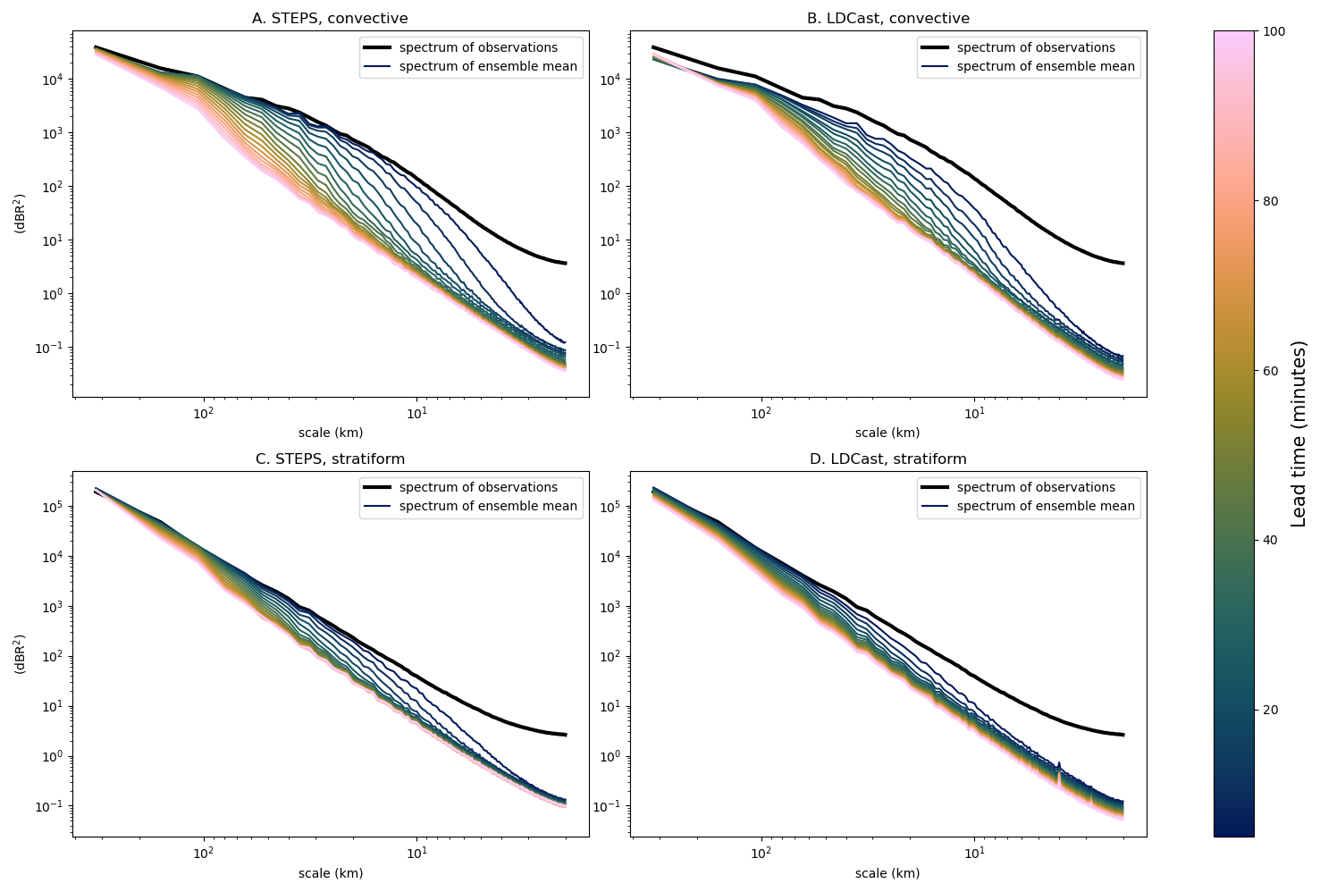
Figure B1 Comparison of power spectra of ensemble means averaged over events (thin colored lines) with the mean power spectrum of observations (thick black lines) for convective and stratiform cases, and for STEPS and LDCast. The color represents the lead time.