Grid-spacing sensitivity of Rossby wave breaking to mesoscale diabatic processes

Forecast busts – episodes of abnormally low forecast skill – remain a persistent challenge for numerical weather prediction despite steady improvements in forecasting skill. Previous studies have highlighted the roles of moist mesoscale processes and diabatically generated potential vorticity (PV) anomalies in triggering rapid error growth and downstream circulation misrepresentation, processes whose representation is highly sensitive to model grid spacing. In this study, we select three events that were classified as forecast busts in the Integrated Forecasting System (IFS) and investigate their sensitivity to horizontal grid spacing. The cases comprise (i) the explosive cyclogenesis of Storm Dennis (February 2020), (ii) a blocking event following the extratropical transition of Hurricane Franklin (September 2023), and (iii) a June 2020 event characterized by ridge amplification due to a warm conveyor belt (WCB) over the North Atlantic. For each case, we use IFS initial conditions and perform global ICON ( Icosahedral Non-hydrostatic model) ensemble forecasts with horizontal grid spacings ranging from 40 to 2.5 km. We evaluate forecast skill against ERA5 reanalysis using anomaly correlation coefficients (ACC) of 500 hPa geopotential height. Across all cases, forecast busts are consistently linked to diabatically generated upper-level negative PV anomalies originating from strong latent heat release in organized convection, including mesoscale convective systems (MCSs), extratropical cyclones, and WCB ascent. These PV anomalies modify the upper-level waveguide, perturb the jet stream, and amplify downstream Rossby wave packets, degrading medium-range predictability. Decreasing horizontal grid spacing systematically improves the representation of diabatic processes, enhances the spatial extent and intensity of upper-level negative PV anomalies, and reduces wave-amplitude error growth. We observe that kilometer-scale simulations with horizontal grid spacing ≤5 km consistently yield the highest forecast skill, with substantial ACC improvements relative to coarser-resolution simulations. All three case studies systematically show that mesoscale diabatic processes are a primary source of forecast error in bust situations, and that kilometer-scale global simulations significantly improve the representation of scale interactions governing Rossby wave amplification. These findings underscore the importance of kilometer-scale simulations for reliably representing scale interactions in strongly diabatic flow regimes. They are not only important for weather forecasting but also for climate simulations which feature long-standing deficiencies in capturing Rossby wave breaking and associate extreme weather events.

1 Introduction

Despite steady improvements in numerical weather prediction (NWP) over recent decades – driven by enhanced observational coverage, improved model capabilities and data assimilation, and increased computational power – forecast skill can still decrease dramatically for specific events (Palmer, 2000; Rodwell et al., 2013). These episodes of abnormally low forecast skill, referred to as ”forecast busts”, are characterized by large discrepancies between predicted and observed atmospheric states and were first documented by Rodwell et al. (2013). Subsequent studies have shown that such busts often arise from the rapid growth and downstream propagation of relatively localized initial errors, leading to large-scale misrepresentations of the atmospheric circulation several days later (Magnusson, 2017; Grams et al., 2018; Lojko et al., 2022). From a broader perspective, forecast busts often occur during periods of large-scale flow reorganization (Hauser et al., 2026). Lillo and Parsons (2017) demonstrated that busts tend to coincide with regime transitions. Under these conditions, even small misrepresentations of moist processes can induce bifurcations in model trajectories, thereby reducing downstream predictability.

The role of moist mesoscale processes has emerged as a recurring theme in the literature on forecast busts. Numerous case studies have demonstrated that, for busts over Europe, errors originating in regions of deep convection – particularly over North America and the North Atlantic can upscale and propagate downstream with the large-scale flow (Martínez-Alvarado et al., 2016; Lojko et al., 2022; Parsons et al., 2019). In particular, the model misrepresentation of mesoscale convective systems (MCSs) has been identified as a major source of initial forecast error. Difficulties in representing the timing, intensity, and organization of convection can lead to substantial errors in diabatic heating (latent heat release from condensation), which in turn modify the upper-level potential vorticity (PV) distribution and the structure of Rossby wave packets (Rodwell et al., 2013; Baumgart et al., 2018; Parsons et al., 2019). Similarly, long lived organized convective systems, such as tropical cyclones, can act as sustained sources of diabatic heating and initiate error growth that propagates downstream in a comparable way to MCSs. It has been shown (Willison et al., 2013) that coarse-resolution models systematically underestimate diabatic heating, thereby failing to capture the resulting downstream ridge amplification and flow evolution.

Beyond MCSs, Warm Conveyor Belts (WCBs) – coherent, rapidly ascending airstreams embedded in extratropical cyclones – have been identified as a particularly effective pathway for upscale error growth. WCB ascent is highly sensitive to environmental baroclinicity, moisture availability, and cloud diabatic processes. Improper representation of diabatic processes such as latent heat release can strongly amplify initial errors and project them onto the upper-tropospheric Rossby wave pattern (Martínez-Alvarado et al., 2016; Grams et al., 2018). Several studies have shown that forecast busts are frequently associated with enhanced WCB activity and strongly amplified large-scale flow patterns, especially over the North Atlantic and Europe (Pickl et al., 2023; Portmann et al., 2020). Blanchard et al. (2021) emphasized the importance of resolving the upper-level negative PV field to accurately represent the jet stream evolution, combining observational data with kilometer-scale regional model simulations. They focused on the role of embedded convection as a source of error in predicting the downstream atmospheric circulation in global models. WCBs have also been shown to be closely linked to Rossby wave breaking (Madonna et al., 2014a), with most WCB outflows co-occurring with PV streamers, underscoring the importance of diabatic processes for downstream wave breaking. Building on these results, Vishnupriya et al. (2025) documented different modes of WCB interaction with the waveguide and showed that WCBs characterized by stronger negative PV anomalies, deeper ascent, and stronger interaction with the waveguide can not only amplify ridges but also contribute to the formation of blocking events and cut-off lows. Together, these studies highlight the central role of WCBs in shaping Rossby wave breaking and downstream flow evolution.

1.1 PV modification by mesoscale processes

Several studies demonstrated that the outflow associated from these mesoscale processes can form pronounced negative PV anomalies that modify the upper-level flow (Grams and Blumer, 2015; Portmann et al., 2020; Bosart et al., 2017; Oertel et al., 2023). These studies not only identified negative PV anomalies but also reported negative PV values in the northern hemisphere. Harvey et al. (2020) examined in detail how negative PV values are generated within the jet environment. Specifically, they showed that latent heat release within a WCB – typically occurring beneath the jet core – induces substantial vertical PV redistribution and lateral PV transport away from the jet axis. This diabatic modification enhances negative PV on the equatorward flank of the jet and produces a characteristic PV dipole structure. The dipole is characterized by low or negative PV on the jet stream flank and positive values further away on the equatorward flank. The negative PV anomaly increases anticyclonic shear, thereby strengthening the jet maximum wind speed and sharpening horizontal PV gradients (Blanchard et al., 2021; Oertel et al., 2020). The magnitude of the negative PV anomaly is directly linked to the intensity of latent heat release; stronger diabatic heating leads to more pronounced PV destruction and thus to more intense negative PV signatures. In this context, negative PV can be interpreted as a dynamical proxy for the strength of convective systems such as MCSs. More intense convection implies enhanced latent heat release and a stronger imprint on the upper-level PV field, often expressed as amplified negative PV anomalies and more distinct dipole structures.

While the above mechanism applies to WCB ascent more generally, embedded convective (quasi-vertical) ascent can amplify this PV redistribution and produce more localized and intense PV anomalies. In particular, the presence of strong vertical wind shear within the WCB is essential: localized diabatic heating in such a sheared environment generates upper-level horizontal PV dipoles centered around the convective updraft and aligned with the horizontal vorticity vector (Oertel et al., 2020). By categorizing WCB trajectories into classical slantwise ascents and quasi-vertical ascents (termed convective ascents), they found that the latter exert a substantially stronger influence on the upper-level PV structure, possibly generating negative PV values and PV dipoles. Thus, embedded convection within WCBs can substantially modulate mesoscale PV structures and, through them, the evolution of the larger-scale flow. Such dipole structures are not unique to WCBs; similar patterns have been documented in association with MCSs (Hitchman and Rowe, 2017; Clarke et al., 2019; Lojko et al., 2022). In cases of intense, localized diabatic heating from rapidly ascending air parcels, horizontal gradients of diabatic heating become dynamically relevant and cannot be neglected, underscoring the importance of fine grid spacing simulations to capture these processes.

These diabatically generated PV anomalies can significantly displace key dynamical features, including jet streams, PV filaments, wave-breaking regions, and cut-off lows, thereby altering downstream Rossby wave propagation and contributing to downstream atmospheric regime shifts and large forecast errors (Davies and Didone, 2013). In particular, low-PV outflows frequently intrude into pre-existing upper-level ridges, promoting ridge amplification and modifying the downstream wave pattern (Grams et al., 2014).

1.2 Aim and outline

The prevalence of moist-process-driven forecast errors highlights persistent limitations in current weather forecasting and climate modeling systems. Many large-scale circulation features – such as atmospheric blocking or Rossby wave breaking – are systematically biased in models operating at coarse horizontal resolution (Davini and D’Andrea, 2020; Luo et al., 2022; Judt and Rios-Berrios, 2021). These biases are closely linked to the inadequate representation of convection and associated diabatic heating since state-of-the-art global weather forecasting and climate modeling systems operating on coarse grid spacing rely on deep convective parameterizations (Prein et al., 2015; Clark et al., 2016).

Importantly, the representation of MCSs and WCBs has been shown to be sensitive to microphysical and convective parameterizations, as well as to horizontal grid spacing, underscoring the difficulty of simulating these processes accurately in coarse-resolution models (Choudhary and Voigt, 2022; Martínez-Alvarado et al., 2014). Several studies have shown that decreasing grid spacing leads to a more realistic representation of WCBs, diabatic heating, cyclone development, MCSs, and deep convection in general, thereby improving the coupling between mesoscale and synoptic-scale dynamics (Willison et al., 2013; Choudhary and Voigt, 2022; Prein et al., 2020). These improvements are particularly relevant for extreme weather events, where intense convection, heavy precipitation, and strong localized diabatic heating are often major sources of forecast error. Despite this growing body of evidence, relatively few studies have systematically assessed the added value of kilometer-scale models for investigating forecast busts. In particular, the degree to which increased model resolution reduces the misrepresentation of mesoscale processes – and constrains the amplification and downstream propagation of forecast errors – has not yet been quantified systematically. Addressing this research gap is increasingly important in a warming climate, where the frequency and intensity of high-impact weather events are projected to increase (Prein et al., 2017).

The objective of this study is to assess if explicitly simulating upstream mesoscale diabatic processes improves non-linear downstream responses, thus improving the forecast skill of a numerical weather prediction model during forecast bust events. Therefore, we perform global ensemble simulations with the ICOsahedral Nonhydrostatic (ICON) model (Zängl et al., 2015) at different grid spacings and test its ability to mitigate recent forecasts busts in the Integrated Forecasting System (IFS) of the European Centre for Medium-Range Weather Forecasts (ECMWF). We evaluate the sensitivity to grid spacing of forecast skill and assess potential sources of improved forecast skill at fine grid spacings.

The main questions that we address in this study are:

1. Can the explicit simulation of upstream mesoscale processes at fine grid spacings in ICON mitigate large-scale forecast errors in IFS?

2. How does horizontal grid spacing modulate the intensity, spatial scale, and vertical structure of moist mesoscale processes?

3. To what extent do these processes modify the upper-level waveguide and how does this affect Rossby wave breaking?

The paper is structured as follows: Sect. 2 introduces the experimental design, the evaluation data and analysis methods. Sect. 3 presents the results from the three case studies of forecast busts analyzed. We discuss the results and compare the cases, and summarize the key findings in Sect. 4.

2 Methods

2.1 Data and model

In this study, both IFS and ICON simulations are evaluated against the fifth generation ECMWF reanalysis dataset, ERA5 (Hersbach et al., 2020). ERA5 has a horizontal grid spacing of approximately 0.25° (spectral resolution T369), 137 vertical levels, and provides data at hourly intervals. We use the ERA5 reanalysis, as it is widely regarded as one of the most reliable reanalysis datasets currently available (Soci et al., 2024). We note, however, that ERA5 is not fully independent from IFS (as it is based from data assimilation using IFS), and this should be taken into account when interpreting the evaluation results. Furthermore, although ERA5 does not explicitly resolve mesoscale dynamics (Li et al., 2024), its data assimilation enables it to capture their upscale impacts on the large-scale flow – which is not the case for IFS, which depends only on initial conditions.

Deterministic and ensemble forecasts from ECMWF are used to identify forecast-bust cases and evaluate forecast skill. The ensemble members are further employed to assess ensemble spread. Since the selected cases are sampled from different years, different operational versions of the IFS with different grid spacings were used. For the first and last cases (in 2020), the ensemble product uses an horizontal grid spacing of approximately 18 km (Cycle 46r1) whereas it is 9 km in the second case study (Cycle 48r1). All ECMWF forecast products are downloaded on a 0.5° × 0.5° latitude–longitude grid, which is sufficient to evaluate the large scale features of the forecast. We also include data from the version 7 of the Integrated Multi-sattelitE Retrievals for GPM (IMERG) product to evaluate precipitation, downloaded on a 0.1° latitude-longitude grid at 30 min time resolution (Huffman et al., 2015).

The IFS forecasts are compared with global ensemble simulations performed using the ICON model. We employ the blue line version of the ICON Model with a GT4Py (GridTools for Python) dynamical core developed in the EXCLAIM project (icon-exclaim v0.2.0) (Dipankar et al., 2026; Lapillonne et al., 2026). For each of the three selected cases, the simulations are integrated for 8 d. ICON is initialized from the IFS analysis, with initial-condition given by the 50 IFS ensemble perturbations. Sea surface temperatures and sea ice data are taken from the Climate Data Record (CDR) produced by the European Space Agency (ESA) Climate Change Initiative Sea Surface Temperature project, which provides daily mean values on a 0.05° latitude-longitude grid (Good and Embury, 2024). The model uses 120 vertical levels extending up to 85 km from the model surface, employing a terrain-following hybrid vertical coordinate with the smooth level vertical (SLEVE) formulation (Schär et al., 2002). Cloud microphysical processes are represented using a one-moment scheme following Seifert (2008) and Doms et al. (2011), which predicts cloud water, cloud ice, snow, graupel, and rain. Radiative transfer is parameterized using the ecRad scheme (Hogan and Bozzo, 2018). Land surface processes are represented by the soil–vegetation–atmosphere transfer model TERRA (Schulz and Vogel, 2020). Soil initial conditions are taken from the IFS. We use the Monitoring Atmospheric Composition and Climate (MACC) ozone climatologies (Katragkou et al., 2015) and the global Max-Planck-Institute Aerosol Climatology version 2 (MAC-v2) dataset with 1° grid spacing at a monthly temporal frequency (Kinne, 2019). This ICON configuration closely resembles that used in the DYAMOND (DYnamics of the Atmospheric general circulation Modeled On Non-hydrostatic Domains) simulations described by Prein et al. (2026) and Pothapakula et al. (2026).

Five horizontal grid spacings are considered: 40 km (R02B06), 20 km (R02B07), 10 km (R02B08), 5 km (R02B09), and 2.5 km (R02B10). This allows to sample a variety of grid spacing, from coarse simulations up to convecting permitting setups. For each selected case, we simulate 50 ensemble members for the grid spacings of 40 and 20 km, 20 members for 10 km, 10 members for 5 km, and between 3 and 5 members for 2.5 km (depending on computing resources). Multiple methods were considered to select the ensembles at fine grid spacings (with configurations with fewer than 50 members) following Khain et al. (2023). To maintain consistent initial conditions across different grid spacings, we matched ensemble members by index (i.e., corresponding ensemble members across all resolution runs share identical initial states). To ensure that these subsets are representative of the full ensemble distribution, we performed bootstrap resampling which confirmed that the selected members capture the overall distribution of forecast skill at day 6. Nevertheless, the reduced number of members at 2.5 km limits the statistical robustness of the results. Overall, the ICON simulation uses the same initial conditions as ECMWF forecast, except for the observational SST and sea ice data, which follow the simulation set-up from Prein et al. (2026). Deep and shallow convection are parameterized in the 40, 20, and 10 km simulations using the Tiedtke-Bechtold bulk mass flux convection scheme (Tiedtke, 1989; Bechtold et al., 2008). In addition, simulations at 10 km grid spacing are performed with only shallow convection parameterized, referred to 10 km conv. off from here on. This configuration is consistent with previous studies (Panosetti et al., 2019, 2020; Vergara-Temprado et al., 2020), which demonstrated that bulk convergence is already resolved at these scales. At grid spacings of 5 and 2.5 km, both convection parameterizations are switched off. Finally, subgrid-scale orographic drag and non-orographic gravity wave drag parameterizations are disabled for the 5 and 2.5 km simulations, in order to use minimal parameterization schemes. All simulations and observational products are interpolated on a 0.5° × 0.5° latitude–longitude grid for evaluation. We perform a conservative remapping for precipitation and vertical velocities and a bilinear remapping for other quantities.

2.2 Forecast busts and evaluation

As described in the previous section, forecast busts are identified using IFS operational forecasts with a 6 d lead time. Following Rodwell et al. (2013), two complementary metrics are applied to define a forecast bust: the anomaly correlation coefficient (ACC) and the root-mean-square error (RMSE) of 500 hPa geopotential height (Z500) over a specified region. A forecast is classified as a bust when the ACC falls below 0.4 and the RMSE exceeds 60 m. The ACC is computed following Hauser et al. (2026)

$$\begin{array}{}\text{(1)}& \mathrm{ACC}={\displaystyle \frac{\frac{\mathrm{1}}{N}{\sum }_{n=\mathrm{1}}^N\left(f_n^{\prime }-{\stackrel{\mathrm{‾}}{f}}^{\prime }\right)\left(a_n^{\prime }-{\stackrel{\mathrm{‾}}{a}}^{\prime }\right)}{\sqrt{\frac{\mathrm{1}}{N}{\sum }_{n=\mathrm{1}}^N{\left(f_n^{\prime }-{\stackrel{\mathrm{‾}}{f}}^{\prime }\right)}^{\mathrm{2}}\frac{\mathrm{1}}{N}{\sum }_{n=\mathrm{1}}^N{\left(a_n^{\prime }-{\stackrel{\mathrm{‾}}{a}}^{\prime }\right)}^{\mathrm{2}}}}},\end{array}$$

where $f_n^{\prime }$ and $a_n^{\prime }$ denote forecast and ERA5 reanalysis anomalies, respectively, and n spans over all considered grid-cells N. These anomalies are obtained by subtracting a 30 d centered running-mean climatology of ERA5 500 hPa geopotential height from 1979 to 2024. The overbars ${\stackrel{\mathrm{‾}}{f}}^{\prime }$ and ${\stackrel{\mathrm{‾}}{a}}^{\prime }$ indicate area-weighted spatial averages over the verification domain (varying between cases). The spatial averages are subtracted from the anomalies to account for possible systematic biases in the input fields. The RMSE is defined as

$$\begin{array}{}\text{(2)}& \mathrm{RMSE}=\sqrt{{\displaystyle \frac{\mathrm{1}}{N}}\sum _{n=\mathrm{1}}^N(f_n-a_n{)}^{\mathrm{2}}},\end{array}$$

where f_n is the forecast value and a_n the reanalysis value at grid-cell n.

Case studies are selected based on the simultaneous satisfaction of these two criteria. Their combined use ensures that busts exhibit both a substantial phase error, as captured by the ACC, and a significant amplitude error, as quantified by the RMSE. This approach targets a specific subset of forecast busts characterized by both phase and amplitude errors, rather than encompassing the full spectrum of forecast busts (such as those driven mainly by phase errors despite high RMSE). For the first case study, the selection criteria were applied to the deterministic IFS forecast to evaluate a classic deterministic forecast bust. For the two subsequent cases, the selection methodology was expanded to additionally require that the IFS ensemble mean satisfied both criteria. This ensures that the poor forecast performance reflects a systematic shift or bias across the entire ensemble distribution, rather than a scenario where the deterministic run simply diverged along a less likely forecast. In addition, we select cases representing different synoptic situations, seasons, and underlying processes to enhance the generalizability of the results. For conciseness, only ACC results are shown, as the RMSE exhibits very similar behavior.

2.3 Warm Conveyor Belts identification

We identify WCBs following a methodology similar to that of Heitmann et al. (2024) and Madonna et al. (2014b). Lagrangian air parcels trajectories are computed using the LAGRANTO analysis tool (Wernli and Davies, 1997; Sprenger and Wernli, 2015) applied to ICON simulated data. Trajectories are initialized every 6 h in time and every 0.5° within a region of interest between 1050 and 790 hPa, with a vertical spacing of 20 hPa, and are propagated 48 h forward in time.

WCB trajectories are defined as air parcels that ascend by at least 600 hPa within 48 h (Wernli and Davies, 1997; Madonna et al., 2014b). The trajectories are further classified by pressure level into inflow (>800 hPa), ascent (800–500 hPa), and outflow (<400 hPa) phases. Based on these WCB trajectories, 2-D WCB masks are constructed following Heitmann et al. (2024). To smooth the resulting masks, each air parcel is inflated into a circle with radius 1° (see Fig. 2 in Heitmann et al., 2024).

We use the ascent area, number of ascending trajectories, and the ascent velocity as proxies for WCB intensity (Choudhary and Voigt, 2022; Heitmann et al., 2024).

2.4 Wave Amplitude Error analysis

To study the upscaling growth of forecast errors in the simulations, we first identify their initial sources. Following Parsons et al. (2019), we quantify a phase-independent error amplitude based on the streamfunction ψ. The streamfunction is derived from the horizontal wind error at upper levels (250 hPa), using ERA5 as the reference dataset. The zonal and meridional wind errors are defined as $u_{\mathrm{e}}=u_{\text{forecast}}-u_{\text{ERA}}$ and $v_{\mathrm{e}}=v_{\text{forecast}}-v_{\text{ERA}}$, respectively. From these, the vorticity error is computed as ${\mathit{\zeta }}_{\mathrm{e}}=\frac{\partial v_{\mathrm{e}}}{\partial x}-\frac{\partial u_{\mathrm{e}}}{\partial y}$. The corresponding error streamfunction, ψ_e is obtained by solving the Poisson equation ∇²ψ_e=ζ_e. Based on these quantities, the Wave-Amplitude Error (WAE) is defined as

$$\begin{array}{}\text{(3)}& E={\displaystyle \frac{\mathrm{1}}{\mathrm{2}}}\left[{\left({\displaystyle \frac{\partial {\mathit{\psi }}_{\mathrm{e}}}{\partial x}}\right)}^{\mathrm{2}}+{\left({\displaystyle \frac{\partial {\mathit{\psi }}_{\mathrm{e}}}{\partial y}}\right)}^{\mathrm{2}}-{\mathit{\psi }}_{\mathrm{e}}\left({\displaystyle \frac{{\partial }^{\mathrm{2}}{\mathit{\psi }}_{\mathrm{e}}}{\partial x^{\mathrm{2}}}}+{\displaystyle \frac{{\partial }^{\mathrm{2}}{\mathit{\psi }}_{\mathrm{e}}}{\partial y^{\mathrm{2}}}}\right)\right],\end{array}$$

This metric isolates the error amplitude independently of its phase and is therefore well suited to tracking wave-like error packets, such as Rossby wave packets. Examining the spatial and temporal evolution of the WAE enables us to pinpoint the location of initial error growth and to trace its subsequent development along the upper-level jet stream.

3 Results

In this section, we present the results of the three case studies. Each case is briefly introduced, followed by an in-depth analysis. A synthesis of the commonalities among the cases is presented in Sect. 4.

3.1 Case 1: Storm Dennis, February 2020

3.1.1 Case overview and error development

As a first case study, we examine the extratropical storm Dennis, one of the deepest Atlantic depressions on record, reaching a minimum pressure of 922 hPa (Davies and Didone, 2013). Dennis formed off the northeastern coast of the United States on 12 February 2020, at 12:00 UTC and propagated across the North Atlantic, merging with an atmospheric river south of Iceland on 15 February. The storm produced the third-highest daily rainfall total in the UK since 1891 (Kendon and McCarthy, 2021).

Figure 1 summarizes the evolution of Storm Dennis and the stages of error growth identified in the simulations. (i) An MCS over the central US (10 February) with intense convection was observed over the southeastern US between 10 and 12 February (day 2 to 4 of the forecast), accompanied by extreme wind, tornadoes, and substantial precipitation (Fig. 1a). (ii) This convection interacted with the jet stream, influencing the exact position and evolution of a trough that formed over northeastern North America. (iii) A subsequent WCB moved across the Atlantic resulting in the formation of a ridge over the UK and Iceland on 14 February 00:00 UTC (6 d of lead time) (Fig. 1b).

This case was poorly forecasted by the deterministic IFS operational forecast, initialized on 8 February at 00:00 UTC, with an ACC value of only 0.29 on 14 February 00:00 UTC. The misrepresentation of the intense convection over the southeastern US in IFS led to errors in its upper-level jet, which caused the misplacement of the trough on 12 February around 12:00–15:00 UTC. Errors in both phase and amplitude grew downstream and led to different storm tracks between ERA5 and IFS (Fig. 2b). The shading shows the differences in mean sea level pressure, reaching values of up to about 40 hPa. Figure 2a shows the 2 PVU contour from ERA5 and the IFS forecast, highlighting differences in the ridge position over Iceland. A trajectory analysis using LAGRANTO (not shown) confirms that the ERA5 WCB outflow was shifted relative to the IFS, directly linking these discrepancies in ridge positioning to differences in the WCB outflow. For illustration, we also include the best and worst member (in terms of ACC) from the ICON ensemble, demonstrating the range of possible upper-level evolutions.

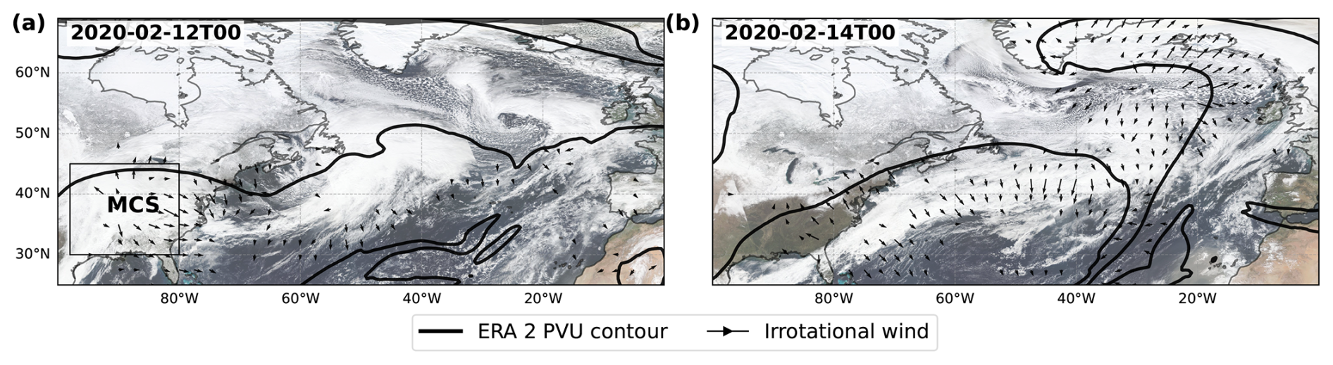
Figure 1 NOAA VIIRS satellite data, overlayed with ERA5 irrotational wind vectors (above 5 m s⁻¹) and potential vorticity (PV; black) at 250 hPa. Data is shown on 12 February at 00:00 UTC (a) and on the 14 at 00:00 UTC (b) (4 and 6 d lead times). The box shown in panel (a) represents the area affected by the MCS, defined as (−105 to 80° W, 30 to 45° N).

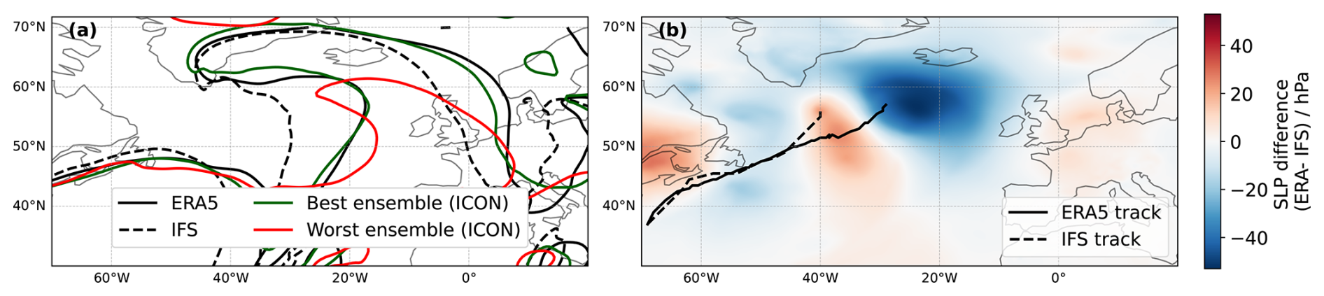
Figure 2 (a) 2 PVU line at 250 hPa for ERA5 (black solid line), IFS forecast (black dashed line), and the best (green) and worst (red) ICON simulations on 14 February 2020 00:00 UTC (6 d lead time). (b) Sea level pressure (SLP) difference between ERA and IFS on 14 February 2020 00:00 UTC (shading), and storm Dennis tracks for IFS (solid black line) and ERA5 (dashed black line) until 14 February 2020 00:00 UTC, tracked from minimum MSLP.

3.1.2 Grid spacing sensitivity

Global ICON ensemble simulations are initialized on 8 February 2020 at 00:00 UTC, six days before the bust happened. From these simulations, the MCS in the southeastern US appears to be a primary source of error. The MCS is identified with the Multi-Object Analysis of Atmospheric Phenomenon (MOAAP) tracking algorithm (Prein et al., 2023) based on IMERG satellite remote sensing data. Figure 3a shows the outline of the identified MCS derived on 10 February at 12:00 UTC (2 d lead time). This long-lived system produces a large area covered with heavy precipitation, indicating substantial latent heat release. Subsequently, the MCS generates negative PV in the upper troposphere, influencing the jet stream and enhancing the WAE at 250 hPa. Individual ensemble members simulate the MCS with varying intensity, which in turn affect the waveguide differently. The variability in MCS representation is reflected in the WAE standard deviation (green shading in Fig. 3a), highlighting an enhanced ensemble spread at the location of the MCS. This MCS is located near the jet stream and injects low-PV air at upper-levels which strengthens the PV gradient and amplifies the downstream Rossby response.

Figure 3b shows the negative PV area on 10 February at 18:00 UTC for ERA5 and ICON, for each ensemble and grid spacing. We use negative PV area as a proxy for MCS intensity: stronger convection leads to enhanced latent heat release and thus more pronounced upper-tropospheric negative PV. Analyzing other variables, such as upper-level divergence and vertical wind speed, produced results consistent with those for negative PV (not shown), highlighting both the consistency of our findings and the suitability of the negative PV area as a proxy for MCS intensity. Finer grid spacing generally increases negative PV area, with ensemble-mean values approaching those of ERA5 in the 2.5 km ensembles. The 40 km ICON ensembles are not shown, as the simulated MCS was weak with very limited negative PV production, highlighting the limitations of coarse grid spacing simulations. Beyond generating stronger outflow, finer grid spacings also produce outflows at higher altitudes than coarser resolutions (not shown). Consistently, the associated heavy precipitation is also better captured at finer grid spacing (Fig. 3c). Reducing the grid spacing from 10 to 5 km largely improves the representation of intense precipitation, while the 2.5 km distribution most closely resembles IMERG observations, despite regridding all the ICON simulations on a 0.5° grid. The results from the negative PV area and precipitation distributions demonstrate that higher-resolution simulations better resolve the intense MCS convection in this region, ultimately leading to lower WAE. Figure A1 shows the percentage of ensemble members exceeding 80 mm of accumulated precipitation over the evaluation period across all model grid spacings (consistent with Fig. 3b). As grid spacing decreases, precipitation becomes less widespread and more spatially localized and intense, bringing the simulations into better agreement with IMERG satellite observations. These findings are not sensitive to the accumulated precipitation threshold and align with the conclusions of the preceding analysis.

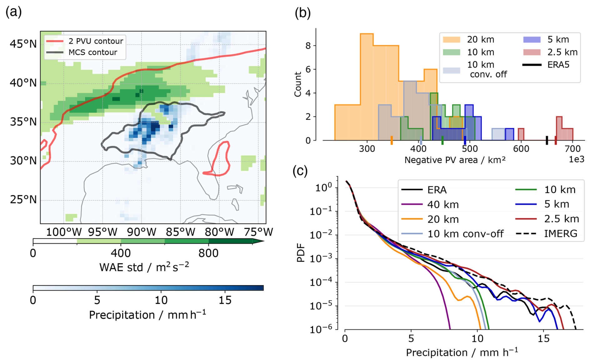
Figure 3 (a) Standard deviation of Wave Amplitude Error (WAE) for all ICON ensembles at a grid spacing of 10 km (green shading), hourly precipitation (blue shading) from IMERG, ERA5 2 PVU contour (red line) and MCS contour (black contour) on 10 February at 12:00 UTC over the southeastern US. (b) Negative PV area at 250 hPa within the box shown in Fig. 1a, on 10 February at 18:00 UTC (2 d lead time). The count corresponds to the number of ensemble members in each bin. The vertical ticks on the x-axis are the means over each grid spacing ensemble as well as ERA5 (black tick). (c) Probability density function (PDF) of precipitation within the domain (105 to 70° W, 25 to 50° N) between the 10 and the 12 February. The PDFs were computed separately and averaged over all ensembles members. We also include ERA5 (solid black line) and IMERG (dashed black line) data.

The explicit simulation of the MCS is crucial, as it influences the position and speed of the jet stream. Errors in their representation are propagated downstream, affecting the formation of a trough along the eastern coast of the US. We find that simulations with lower WAE tend to produce deeper troughs. To quantify this relationship, we compute the mean PV at 250 hPa within the trough region on 12 February at 15:00 UTC and correlate it with the mean WAE at the same time (Fig. A2). A negative correlation of −0.68 indicates that simulations with higher WAE generally correspond to weaker troughs. Furthermore, we also find a correlation of −0.65 between the WAE on 12 February at 15:00 UTC (2 d lead time), and the ACC on day 6 (Fig. A3), demonstrating that the error propagates downstream: simulations with lower initial WAE tend to achieve higher ACC at later lead times.

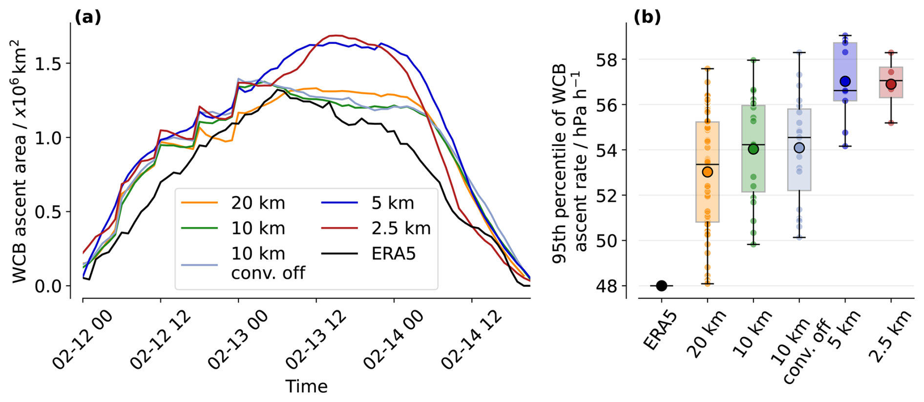
Figure 4 (a) WCB ascent area over time from ERA5 (solid black line) and the ICON simulations (colored lines). Ensemble mean values are shown for the ICON simulations. The area was computed using the Eulerian mask described in the Sect. 2. (b) Box plots of 95th percentile of ascent velocity for each ensemble and each grid spacing and ERA5.

This error, both in phase and amplitude of the trough, creates initial conditions differences in the formation and development of the WCB whose outflow contributes to the formation of the ridge on day 6 of the forecast (Fig. 1b). To evaluate the WCB, we analyze its ascent area and ascent velocity as proxies for the spatial extent and intensity of ascent (Choudhary and Voigt, 2022; Lojko et al., 2025a) (Fig. 4). We find a systematic increase in ascent velocity (Fig. 4b) in the 95th percentile of fastest ascending trajectories, indicating that higher horizontal resolution captures more intense ascent even when coarsened to a 0.5° grid. This behavior is consistent with the findings of Choudhary and Voigt (2022), who reported enhanced diabatic heating at finer grid spacings. In contrast, we find only a weak sensitivity of ascent velocity to the parameterization of deep convection in the 10 km simulations. Moreover, ERA5 consistently underestimate the ascent velocity compared to ICON simulations. Evaluating the ascent area of the WCBs across different grid spacings leads to similar grid spacing sensitivity. Up until day 6 of the forecast (14 February), the ascent area increases systematically with decreasing grid spacing (Fig. 4a). Once again, the ERA5 values are consistently lower than the ICON simulations. This discrepancy may arise because ERA5 underestimates vertical velocities, resulting in a smaller ascent area. Such discrepancies in ERA5 vertical velocities have previously been reported by Uma et al. (2021). However, we did not observe any differences in WCB outflow height with varying grid spacings. Overall, these results indicate that finer grid spacings resolve more intense ascent and larger WCB. This WCB contributes to the formation of a ridge on forecast day 6, leading to a large error in the IFS forecast of the Z500 field.

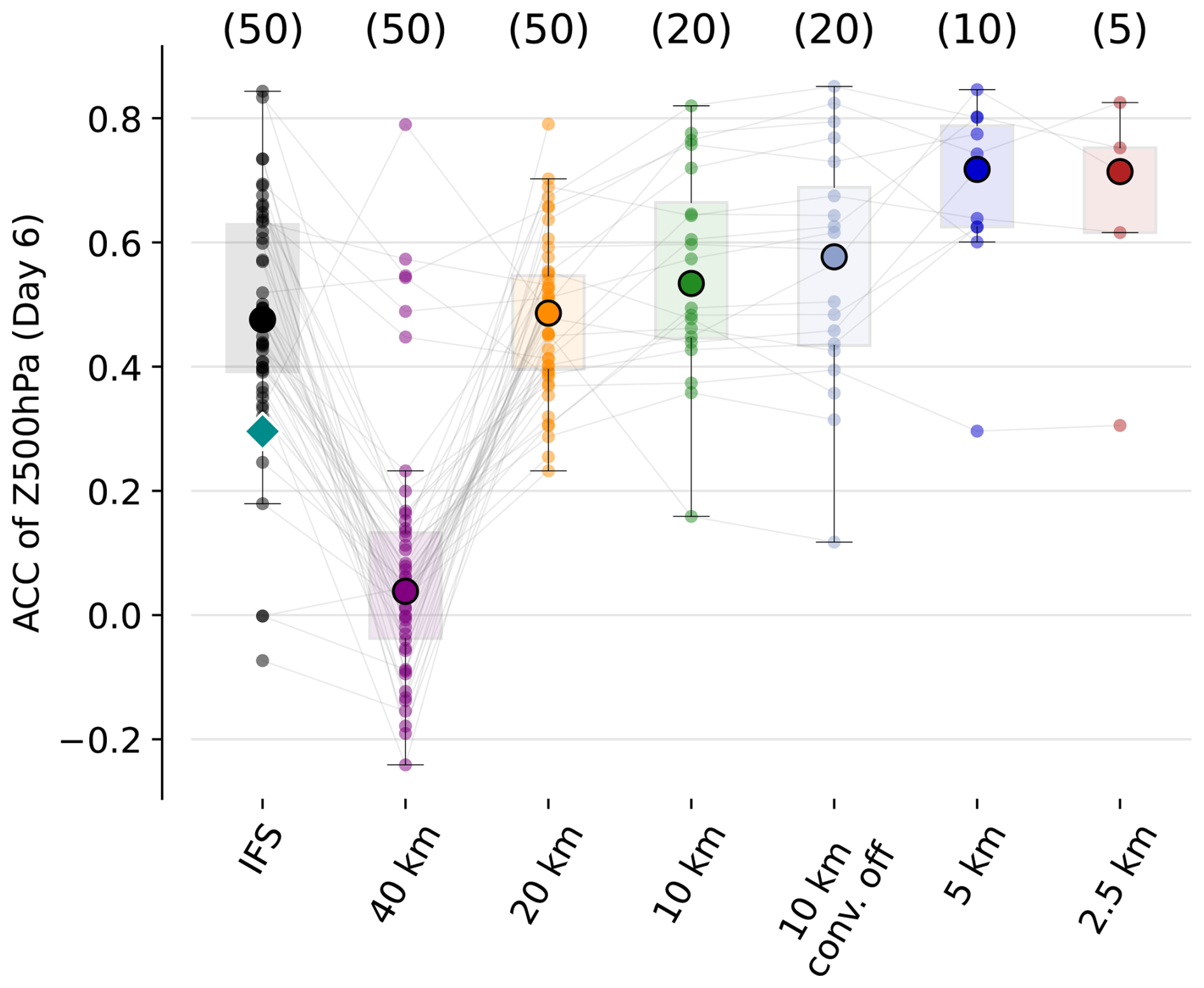
Figure 5 Anomaly correlation coefficient (ACC) over the North Atlantic/European sector (−13 to 40° E, 35 to 75° N) on 14 February 2020, 00:00 UTC computed for each ensemble member (spread) across all grid spacings ICON and for IFS. The larger round markers show the ensemble median, boxes show the interquartile range (25th–75th percentiles), and whiskers extend to 1.5 times the interquartile range of ensemble ACC values. The colored small circles indicate individual ensemble members. The dark cyan diamond shows the deterministic forecast of IFS. The thin black lines between markers connect simulations with the same initial conditions. Numbers in parentheses indicate the number of ensembles at each grid spacing.

The dynamical error growth described above is reflected in the day 6 ACC over the North Atlantic/European sector (−13 to 40° E, 35 to 75° N). Figure 5 shows the ACC for all ICON simulations, together with the IFS ensemble forecasts. As noted earlier, the deterministic IFS forecast exhibits an ACC substantially lower than the ensemble median. At 40 km resolution, ICON yields very low ACC values (slightly above zero). These ensemble members fail to simulate the MCS and trough development and therefore do not capture the subsequent WCB evolution and ridge amplification. Reducing the grid spacing to 20 km increases the ACC to values comparable to the IFS ensemble median, with this improvement being statistically significant using a bootstrap test with 95 % confidence. Further refining the resolution to 10 km provides only marginal additional improvement. Turning off the parameterization of deep convection at 10 km leads to a slight increase in forecast quality (from 0.53 to 0.58) but also a larger forecast spread. A more pronounced improvement is obtained at kilometer-scale grid spacings of 5 and 2.5 km, being statistically significant, with only minor differences between these two grid spacings. The thin black lines connecting ensemble members across different grid spacing show the importance of initial conditions: members exhibiting low ACC at coarse resolution generally retain comparatively low ACC values at finer resolutions. For most members with the same initial conditions, we observe a gradual increase in ACC as the grid spacing decreases. While a few coarse-grid-spacing simulations (e.g., 40 or 20 km) also exhibit high ACC values, these cases do not reflect an improved representation of the underlying physical processes. They are rather outliers within the ensemble where specific initial-condition perturbations compensated for errors related to the coarse resolution, driving the correct synoptic development. Therefore, while the resulting forecast is accurate, it is achieved for the wrong physical reasons and lacks the consistent physical fidelity seen at km-scale grid spacings.

3.2 Case 2: Atmospheric blocking, September 2023

3.2.1 Case overview and error development

As a second case study, we investigate the extreme weather event that affected Europe in early September 2023, which followed the northward propagation and extratropical transition of Hurricane Franklin in late August. Franklin formed on 20 August over the eastern Caribbean Sea and moved poleward, undergoing extratropical transition as it reached the mid-latitudes. The resulting extratropical cyclone interacted with the upper-level jet stream, promoting the development of a pronounced warm conveyor belt, which contributed to Rossby wave breaking in early September. This wave breaking led to the establishment of a persistent omega blocking pattern, associated with the formation of two low-pressure systems: one over the Iberian Peninsula and another over the Mediterranean Sea (Couto et al., 2024; Flaounas et al., 2025). The Mediterranean cyclone intensified and evolved into Storm Daniel, causing catastrophic impacts across Greece, Bulgaria, Turkey, and Libya (UNHCR, 2024).

As in the previous case, the IFS deterministic forecast failed to accurately predict the blocking event. When initialized on 30 August 2023, the operational forecast reached an ACC of −0.24 on day 6 (5 September), while the ensemble median was 0.11, well below the 0.4 threshold. Figure 6a shows a geopotential contour at 500 hPa for the deterministic IFS forecast, highlighting the discrepancies with the ERA5 reanalysis. The forecast displayed a pronounced wave activity, with a ridge over Europe and troughs over the Iberian Peninsula and over Turkey and Greece. However, both the trough and ridge amplitudes were underestimated. The figure also includes contours from the best ICON ensemble member, that successfully captures the Rossby wave breaking and the subsequent block formation, and the worst one, exhibiting weak wave activity, limited wave breaking, and no ridge amplification. The forecast bust from IFS resulted in substantial differences in 850 hPa temperature, displayed in Fig. 6b. In the forecast, the ridge did not extend as far north as in ERA5, leading to pronounced negative temperature anomalies over northern Europe. Moreover, the ridge is displaced eastward relative to the reanalysis, producing positive temperature anomalies across much of the Mediterranean region. As previously, we analyze the different stages of error growth and investigate the sensitivity of the results to horizontal grid spacing using global ICON ensemble simulations.

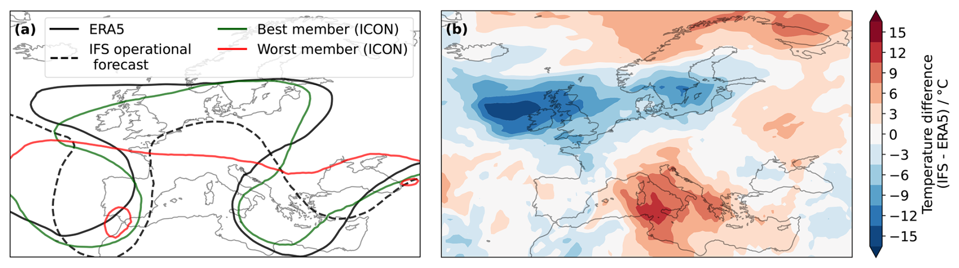
Figure 6 (a) Geopotential contour of 5800 m at 500 hPa for ERA5 (black solid line), IFS forecast (black dashed line), and the best (green line) and worst (red line) ICON ensemble members (all grid spacing considered) on 5 September 2023 00:00 UTC. (b) Temperature difference (IFS–ERA5) at 850 hPa on 5 September 2023 00:00 UTC (6 d lead time).

3.2.2 Cyclone–jet stream interactions

To study error growth in this case, we focus on three main aspects identified as potential sources and drivers of error growth: cyclone Franklin‘s track after its extratropical transition, its interaction with the jet stream, and the subsequent Rossby wave breaking.

Figure 7a shows cyclone Franklin tracks, following its sea level pressure minima, for all ensemble members and horizontal grid spacings up to 4 September 2023. To characterize the diversity of cyclone evolutions, we apply a K-means clustering algorithm to the cyclone tracks. To this end, each track is represented by a vector spanning from the initial cyclone position at the beginning of the simulation (30 August) to its position at the end of the tracking period. From this, three distinct clusters are identified. The first cluster comprises cyclones that propagate slowly and remain nearly stationary; hereafter, this cluster is referred to as the Quasi-stationary cluster. The second cluster follows a north-eastward (NE) track with a moderate propagation speed and exhibits a path closely resembling the ERA5 cyclone track; this cluster is referred to as the Moderate NE cluster. The third cluster comprises cyclones that move much more rapidly towards higher latitudes and is referred to as the Strong poleward cluster.

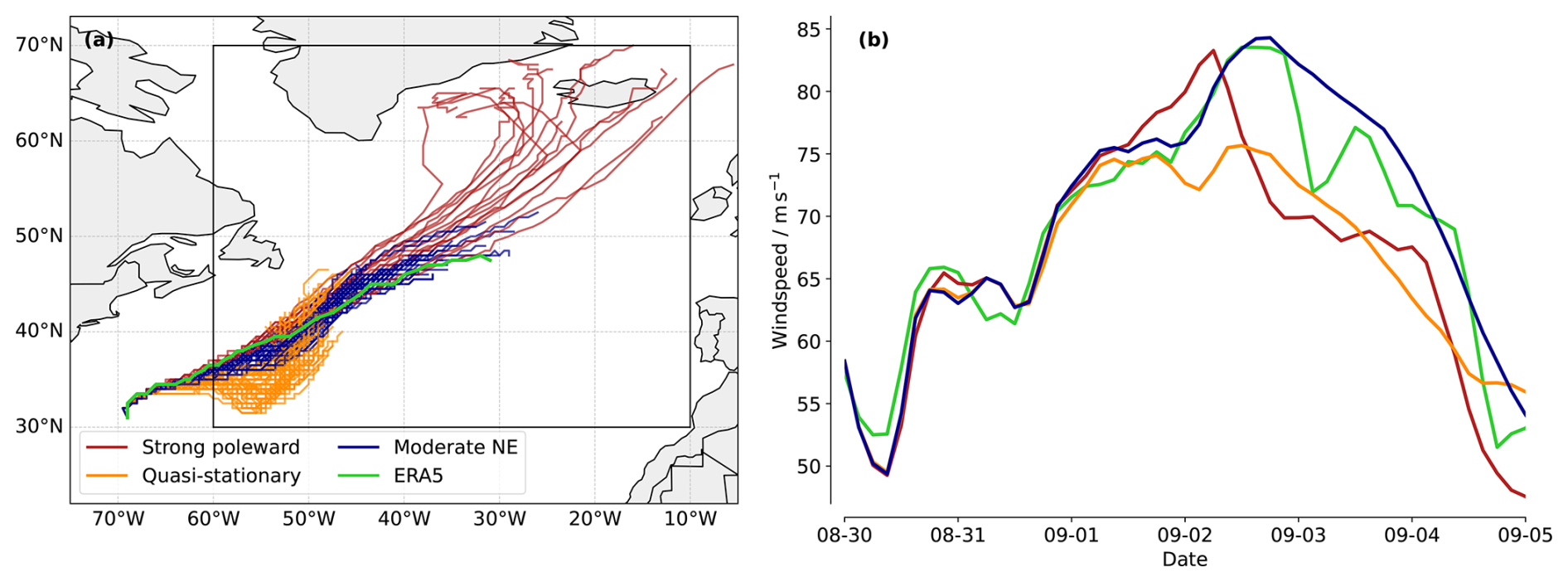
Figure 7 (a) Cyclone tracks for all ICON simulations (all ensemble members and grid spacings) clustered into three subsets. The cyclones were tracked until 4 September 2023 (5 d lead time). (b) Cluster means of the 99th percentile of wind speed in the area where the cyclone interacts with the jet stream over time (−60 to −10° W, 30 to 70° N), shown as a thin black box in panel (a). The green line corresponds to ERA5.

Figure 7a shows that the tracks belonging to the Moderate NE cluster most closely resemble the ERA5 track (green line). Consistently, this cluster exhibits the highest forecast skill over an extended North Atlantic/European sector (−30 to 40° E, 25 to 75° N) on 5 September 2023 00:00 UTC, with a mean ACC (averaged over all ensembles and grid spacings) of 0.52, compared to 0.12 and 0.34 for the quasi-stationary and strong poleward clusters, respectively.

The cyclone track plays a central role in the downstream dynamics that ultimately lead to the forecast bust on September 5th. Previous studies have shown that when a cyclone propagates poleward and its motion is in phase with the jet stream, it can interact with the jet through an upper-level negative diabatically produced PV anomaly, promoting strong ridge amplification and anticyclonic Rossby wave breaking downstream (Wernli and Gray, 2024; Riemer and Jones, 2010; Grams and Archambault, 2016). Figure 7b shows the 99th percentile of 250 hPa wind speed for each cluster and for ERA5, computed within the area shown in Figure 7a. This metric robustly captures the peak wind speeds along the jet stream core, consistently occurring near the cyclone. occurring near the cyclone. Cyclones in the Quasi-stationary cluster do not propagate far enough north to efficiently interact with the jet stream, resulting in a substantially weaker jet and wind speeds that remain well below those in ERA5. In contrast, cyclones in the Strong poleward cluster exhibit a pronounced wind speed maximum around 2 September, corresponding to the time at which the cyclone interacted with the jet stream. This highlights the role of upper-level divergence in temporarily strengthening the jet. However, due to their rapid propagation, these cyclones interact with the jet stream over a relatively short time period, which may explain the subsequent decrease in wind speed after 2 September. Finally, the Moderate NE cluster shows mean wind speeds that closely resemble those in ERA5. These cyclones follow the jet stream axis and continuously inject negative PV into the upper troposphere, thereby supporting jet acceleration until the cyclone weakens. This interpretation is supported by Fig. A5, which shows the distances of the cyclones to the jet streams over time for all simulations at all resolutions. While the Strong poleward cyclones approach the jet rapidly before moving northward, and the Quasi stationary are continuously further away, the Moderate NE cluster consistently mirrors the ERA5 trajectory – thus mirroring their comparable wind profiles. Overall, these results are consistent with Keller et al. (2026), who emphasized how sensitive the forecast of this blocking pattern (and the subsequent formation of Storm Daniel) was to the position of Hurricane Franklin.

3.2.3 Grid spacing sensitivity

Only 28 % of IFS ensemble members forecasted the cyclone's track correctly (as they fall in the Moderate NE cluster), highlighting the overall limited forecast skill of this case from this forecasting system. For ICON, in addition to the inter-member variability in cyclone-track representation and jet interaction presented previously, we identify a sensitivity to horizontal grid spacing. Figure 8 shows the percentage of simulations falling in each cluster for every grid spacing. As the horizontal grid spacing decreases from 40 to 10 km, the proportion of ensemble members falling into the Moderate NE cluster first slightly drops but then increases back to about 40 %. A chi-square test shows that differences in cluster frequencies are only statistically significant between 20 and 5 km. Due to low ensemble members at 2.5 km the increase is not statistically significant.

We also detect a clear resolution dependence in the magnitude of diabatically generated negative PV anomalies associated with each cyclone. Figure A4 presents the distribution of negative PV area on 2 September at 15:00 UTC for all grid spacings. As in the first case, the negative PV area systematically increases with decreasing grid spacing, indicating that finer resolutions enhance the production and export of upper-level low-PV air.

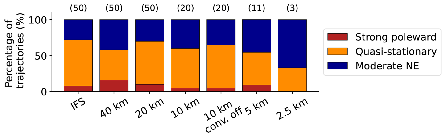
Figure 8 Percentages of simulations with cyclones in each cluster for IFS ensembles and for all ICON ensembles at each grid spacing. Numbers in parentheses indicate the number of ensembles at each grid spacing.

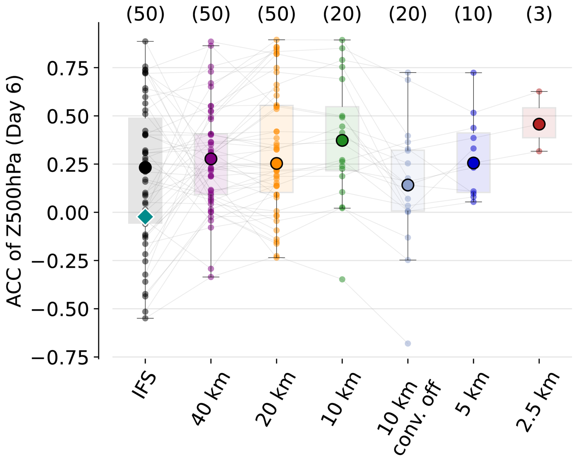
Figure 9 As Fig. 5 but for the second case with evaluation on 5 September 2023 00:00 UTC within (−30 to 40° E, 25 to 75° N).

These improvements in cyclone tracks and their interaction with the jet stream at finer grid spacings lead to a higher ACC on day 6 on the extended North Atlantic/European sector, as illustrated in Fig. 9. At 40 km, the median ACC of ICON is slightly higher than that of the IFS ensemble (0.08 larger), but a bootstrapping test indicates that these differences are not statistically significant. The differences between IFS and ICON become statistically significant at a grid spacing of 10 km. Turning off the parameterization of deep convection at 10 km, leads to a sharp drop in ACC (from 0.38 to 0.14), which mirrors the decrease in cyclones in the Moderate NE cluster previously shown in Fig. 8. These results highlight that some findings of this study are case-dependent. In contrast to the first case, which shows little sensitivity to the deep convection scheme at a grid spacing of 10 km, the second case exhibits a clear drop in skill when it is turned off, suggesting that for processes involved in this case the parameterization of deep convection at such grid spacings can be beneficial. Further reducing the grid spacing recovers this loss, with ACC reaching 0.45 at 2.5 km. However, due to the limited ensemble amount, this increase is not statistically significant. The importance of initial conditions is reflected by ensembles that exhibit very low ACC at coarse grid spacing, and maintain this low ACC at finer ones, with only minimal crossover between the thin lines. Categorizing the simulations into parameterized and explicit convection reveals that both groups show improved ACC with finer grid spacing. Nevertheless, both attain similar ACC performance at 10 and 2.5 km resolution. With only three members, the ACC distribution of the 2.5 km ensemble is insufficiently sampled, and a larger ensemble would likely show higher-performing individual members. The overall low mean ACC, as well as little improvements with decreasing grid spacing, highlight the low predictability of the system. Ultimately, this case study illustrates the inherently low predictability of certain forecast busts, demonstrating that decreasing grid spacing alone is insufficient to fully overcome these initial-condition constraints. Dolores-Tesillos et al. (2026) also documented the persistent difficulty in simulating atmospheric blocking, confirming that reducing grid spacing alone does not resolve these representation errors.

3.3 Case 3: Warm Conveyor Belt ridge amplification, June 2020

3.3.1 Case overview and error development

As a third case study, we examine a forecast bust from early June 2020 associated with severe convective storms and damaging winds over the central United States. The event was driven by intense embedded convection within a WCB over the Rockies and central US between 5 and 9 June. The strong upper-level outflow from this WCB altered the downstream waveguide and triggered Rossby wave breaking along the East Coast. This wave breaking led to the formation of a cut-off low over the western North Atlantic and was followed by the development of a secondary WCB, whose outflow contributed to ridge amplification over the North Atlantic in subsequent days.

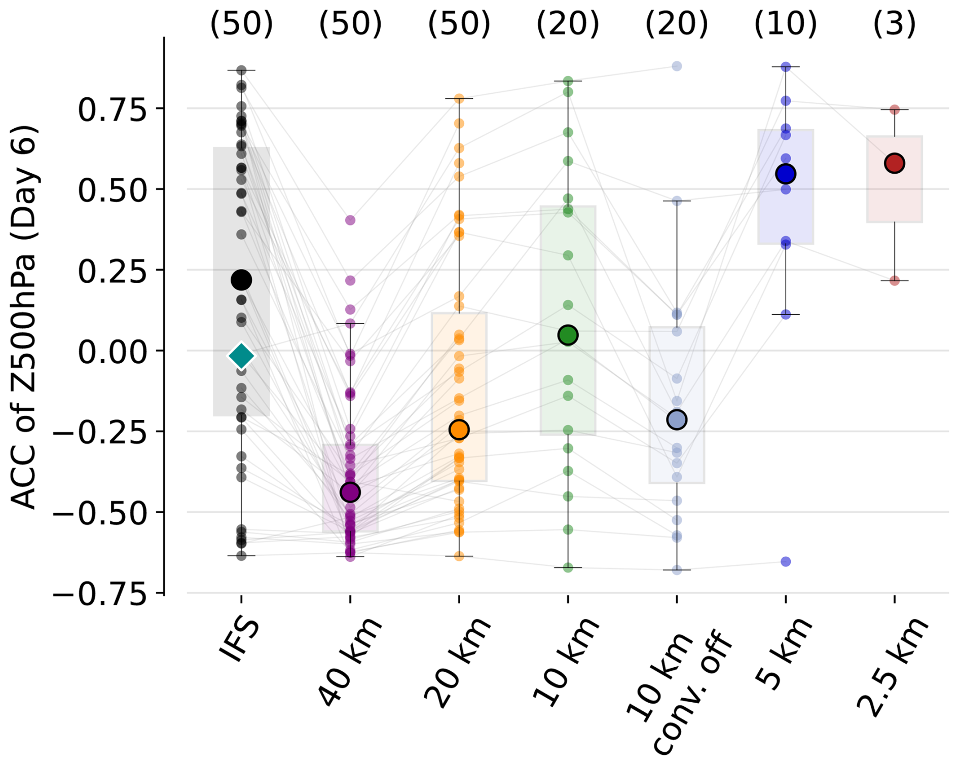
As in the previous cases, the IFS forecast failed to capture the large-scale flow evolution. With initialization on 5 June 2020, the deterministic forecast reached an ACC of −0.02 and with an ensemble median of 0.22 within the Atlantic sector (−75 to 0° E, 35 to 75° N), well below the forecast bust threshold of 0.4. The forecast underestimated the ridge amplification downstream of the WCB outflow and produced a much more zonal Z500 flow pattern compared to ERA5 (Fig. 10a). In particular, the ridge building south of Iceland, dynamically linked to the WCB outflow, was largely absent in the forecast (Fig. 10b). For comparison, the best and worst ICON ensemble members are shown in Fig. 10a. The former successfully captures the downstream ridge amplification, and the latter exhibits weak wave amplification and limited ridge development, highlighting the variability across ensemble members.

We identify three main stages of error growth. First, errors arise in the representation of the initial WCB outflow over the central US. Second, these perturbations propagate downstream, leading to phase shifts in Rossby wave breaking and in the development of the trough along the East Coast. Finally, these errors affect the trajectories of the subsequent WCB, resulting in different outflow regions over the North-Atlantic.

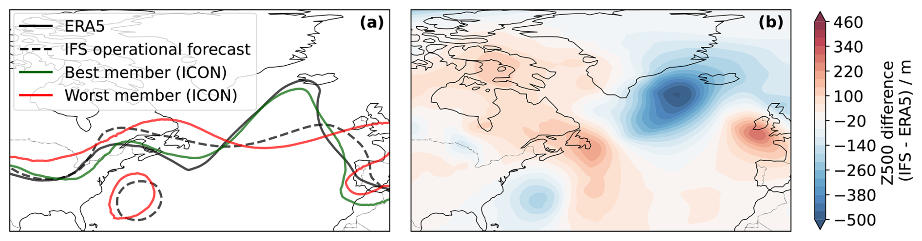
Figure 10 (a) Geopotential contour of 5800 m at 500 hPa for ERA5 (black solid line), IFS forecast (black dashed line), and the best (green) and worst (red) ICON ensemble members (all grid spacings considered) on 11 June 2020 00:00 UTC. (b) Z500 difference (IFS–ERA5) on 11 June 2020 00:00 UTC (6 d lead time).

3.3.2 Grid spacing dependence

As in the first case, we examine the generation of negative PV in the upper-level outflow and its impact on the downstream jet stream evolution. In contrast to the previous case, where MCSs were the primary source of diabatic PV modification, negative upper-level PV here arises from the outflow of a WCB. However, the impact on the WAE at 250 hPa is comparable (not shown), with enhanced WAE in the affected region reflecting the intensified diabatic forcing associated with the WCB convection. Figure 11a displays the negative PV area at 15:00 UTC on 8 June for ERA5 and for the ICON simulations across all ensemble members and grid spacings (within 110 to 65° W, 40 to 60° N). The behavior closely mirrors that found in the first two cases (Figs. 3b and A4): the negative PV area increases systematically with decreasing grid spacing. This robust resolution dependence underscores the ability of higher-resolution simulations to represent intense diabatic ascent and the associated production and export of negative PV into the upper troposphere.

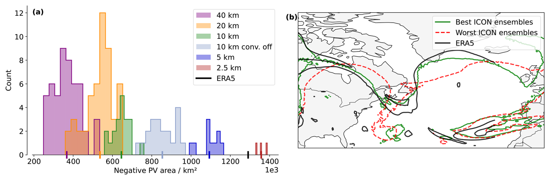
Figure 11 (a) Similar as Fig. 3b on the 8 June, 15:00 UTC considering grid cells within 110 to 65° W, 40 to 60° N. (b) Z500 contour at 5800 m on 9 June, 15:00 UTC (4 d lead time) for ERA5, and the mean of the 5 best- and 5 worst-performing (in terms of ACC on day 6) ICON ensembles.

As noted previously, errors in the representation of the initial WCB outflow affect the downstream jet stream evolution and the Rossby wave breaking on 11 June. We do not observe any substantial changes in wind speed associated with the negative PV, but rather a shift in the phase and amplitude of the wave and the breaking. Figure 11b shows the mean Z500 at 5800 m on 11 June for the five best- and worst-performing ICON ensemble members (independent of grid spacing) compared to ERA5. The best performing ensembles members exhibit a more pronounced wave activity over the Northern Atlantic, which resembles the ERA5 Z500 profile. In contrast, the worst ensembles feature a PV cut-off low positioned too far west and a more zonal Z500 pattern over the North Atlantic. Varying the number of ensemble members does not affect the results, which remain consistent across all tested configurations. These differences in trough position influence the WCB formation, which later amplifies the ridge in the forecast. Figure 12 shows, for each grid spacing ensemble, the percentage of ensemble members with a WCB outflow within a given region. At coarse grid spacings (40 and 20 km), some ensembles fail to produce a WCB, resulting in generally low outflow occurrence across the domain. As the grid spacing decreases, the overall outflow percentages increase, and the spatial structure better resembles the ERA5 reference. Across most grid spacings, two clusters emerge: one producing overly zonal outflow and another that agrees more closely with the ERA5 outflow over southern Greenland. With increasing resolution, the frequency of members in the second cluster increases. However, when the deep-convection parameterization is switched off at 10 km, the outflow becomes more zonal and fewer trajectories reach higher latitudes. The issue is largely resolved at 5 km, where the WCB outflow patterns closely match the ERA5 data. At this grid spacing, the simulations more accurately capture downstream ridge amplification over the North Atlantic and agree well with ERA5. At 2.5 km, the two previously identified clusters become clearly visible. Given that only three ensemble members were performed at this grid spacing, these differences should be interpreted with caution. Nevertheless, all members exhibit a cyclonic outflow branch directed toward Greenland, with frequencies reaching 100 %, contributing to ridge amplification.

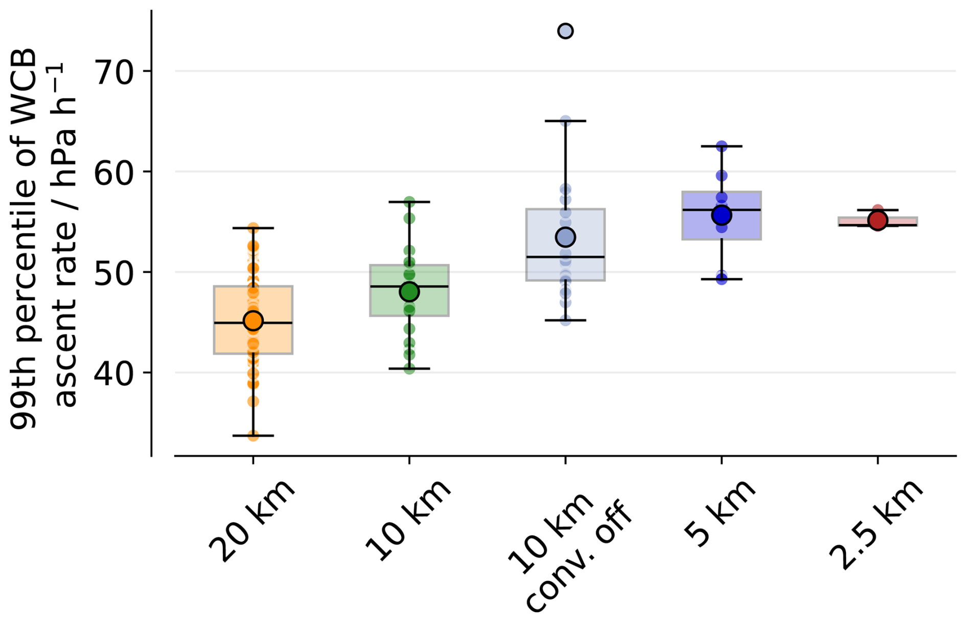
There is also a large horizontal grid spacing dependency of ascent velocity in the WCB consistent with other cases. Figure A6 presents the 99th percentile of ascent velocity for all ensemble members at each grid spacing, revealing a systematic increase as grid spacing decreases.

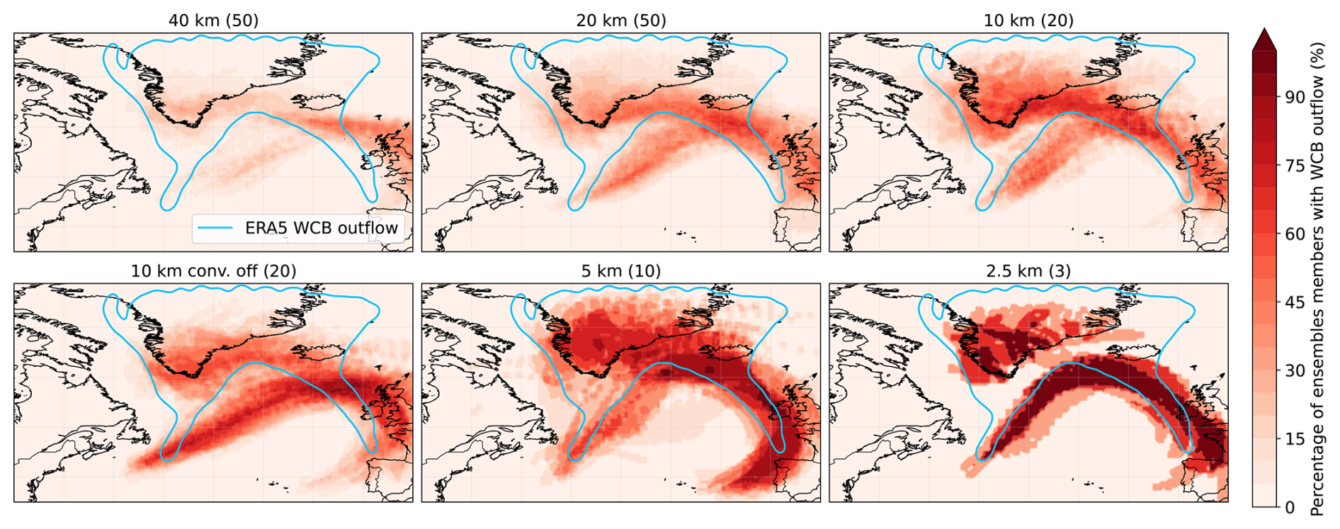
Figure 12 Percentage of ensemble members with WCB outflow within a given grid-cell. For each ensemble, we select all trajectories once they ascend above 400 hPa and construct a binary mask representing the spatial extent of the WCB outflow. Combining all ensemble members, the fraction of members that produce outflow in each grid-cell is computed. The numbers of ensemble members for each grid spacing is indicated in parenthesis. For reference, the ERA5 WCB outflow is overlaid as a light-blue contour.

Figure 13 shows the ACC at day 6, within the North Atlantic domain defined previously, for all ensembles and grid spacings, alongside the corresponding IFS results. The ensemble members in IFS display two clusters of skill score, with large differences depending on initial conditions. One cluster exhibits low values (below 0), while the other exceeds 0.4. This bimodal distribution suggests low predictability for this event, indicating that a skillful forecast is highly dependent on specific initial conditions. A systematic increase in ACC is observed as the grid spacing is reduced from 40 to 10 km. The median ACC increases systematically from −0.43 at 40 km to −0.25 at 20 km and further to 0.09 at 10 km. These improvements were evaluated using a bootstrap approach and are statistically significant with 95 % confidence. Only at 10 km are the differences between IFS and ICON not significant, with both showing similar ACC values. Consistent with the second case, disabling the deep-convection parameterization substantially degrades forecast performance. In contrast to the previous cases, however, the IFS ensemble median outperforms the ICON ensemble means up to a grid spacing of 5 km. Only at a grid spacing of 5 km does the ensemble mean ACC exceed the threshold of 0.4. At kilometer-scale grid spacings, the small number of ensemble members prevents statistically significant comparisons, although high ACC values are observed. No major difference occurs between the 5 and 2.5 km simulations. Overall, this case exhibits a substantially stronger sensitivity to horizontal resolution, with the skill improvement from 40 to 2.5 km being considerably larger than in the previous cases.

Figure 13 As Fig. 5 but for the third case with evaluation on 11 June 2020 00:00 UTC within (−75 to 0° E, 35 to 75° N).

4 Discussion and Conclusion

We investigate the sensitivity of ICON ensemble forecasts to horizontal grid spacing across three distinct IFS forecast busts. The cases feature a large variety of synoptic regimes: intense cyclogenesis associated with Storm Dennis, atmospheric blocking linked to Hurricane Franklin, and a WCB-driven ridge amplification. In all cases, diabatically generated upper-level negative PV plays a central role. This negative PV, generated from MCSs, WCB outflows or extratropical cyclones, intensifies the meridional PV gradient. This strengthening of the gradient promotes Rossby wave amplification and, in some cases, wave breaking. Despite the differing meteorological settings, the underlying error mechanism is remarkably consistent: diabatically driven PV redistribution perturbs the jet, which subsequently amplifies downstream flow errors.

These findings are consistent with previous work. Lojko et al. (2022) demonstrated how MCS-induced negative PV anomalies affect jet amplitude and phase, while Blanchard et al. (2021) highlighted the role of mid-level convection within WCBs in accelerating the jet via PV dipole formation. Similarly, Baumgart et al. (2018) demonstrated that forecast errors in upper-tropospheric divergent flow primarily originate from misrepresented mesoscale diabatic processes. When models fail to accurately resolve this diabatic outflow, these errors project onto the tropopause and amplify downstream through nonlinear Rossby wave dynamics, ultimately degrading medium-range forecast skill. Our results extend these insights by showing that multiple diabatic sources – including MCSs, cyclones, and WCB ascent – can reinforce the jet stream and amplify ridge development through similar PV-mediated mechanisms, and that an improved representation of these upstream process chains is closely associated with enhanced forecast skill downstream. Importantly, we do not expect shallow convection or isolated deep convection and short-lived MCSs to create major changes in Rossby waves, but focus instead on large MCS that can impact large-scale dynamics.

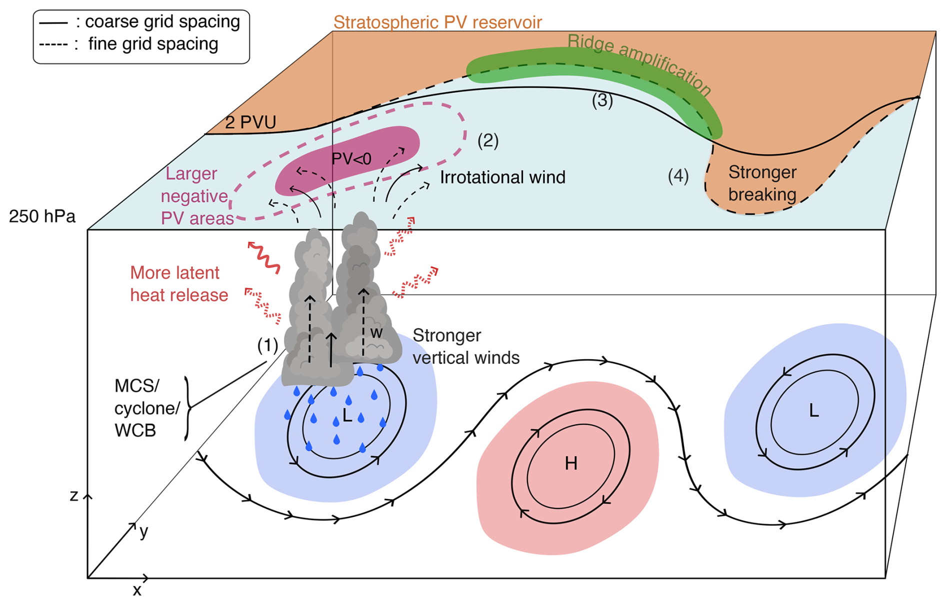
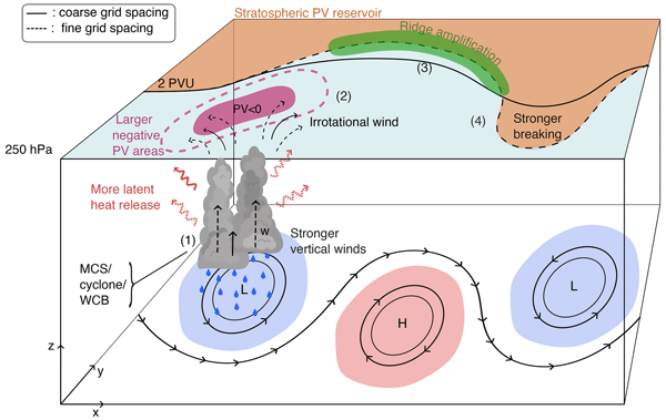
Figure 14 Overview schematic illustrating the key processes identified in the three analyzed cases as well as their differences between coarse grid spacing (solid line) and fine grid spacing (dashed line). (1) Organized convection (MCSs, cyclones, or WCBs) with important vertical winds (w) releases latent heat, produces heavy precipitation and a pronounced upper-level outflow, diagnosed by enhanced irrotational wind at 250 hPa (2). The associated upper-level negative PV anomaly perturbs the jet stream (3) and can promote Rossby wave breaking (4).

Model horizontal grid spacing systematically affects forecast performance and key mesoscale processes across all three cases. Figure 14 summarizes the key processes analyzed in this study as well as their interaction. Following our schematic, reducing horizontal grid spacing consistently:

• Enhances the representation of mesoscale dynamic and diabatic processes: MCSs exhibit stronger convection, enhanced vertical velocities, WCB ascent rates are higher, and intense precipitation is more realistically simulated, consistent with previous literature (Prein et al., 2020, 2025). Fine grid spacing simulations also better capture feature – jet interactions, promoting ridge amplification and Rossby Wave Breaking.

• Increases the magnitude and spatial extent of upper-level negative PV production, leading to improved agreement with ERA5. These improvements are consistent with previous studies (Blanchard et al., 2021), possibly reflecting a more accurate representation of horizontal latent heating gradients.

• Improves downstream forecast skill: the median ACC at day 6 consistently increases with finer grid spacing, as does the likelihood of exceeding the threshold for forecast busts (ACC=0.4). These improvements are statistically significant and particularly pronounced as grid spacing approaches kilometer-scales (≤5 km). However, despite the general increase in ACC at finer grid spacings, mean skill scores for certain events remain very low even at kilometer scales, highlighting the inherently low predictability of some forecast busts.

Importantly, these improvements with decreasing grid spacing are not confined to the immediate region of convection but propagate upscale via Rossby wave dynamics, demonstrating how more accurately simulating small-scale dynamic and diabatic processes influences large-scale circulation predictability. While investigating three detailed forecast events – each representing a distinct flow pattern – provides valuable physical insights and represents a major step forward, generalizing these findings should be done with caution until validated across a broader sample of cases. The sensitivity to the parameterization of convection further underscores this scale dependence. Disabling the deep convection parameterization at 10 km grid spacing yielded case-dependent results: slight improvement in one case but substantial degradation in others. This suggests that the benefit of explicit convection at this grid spacing depends strongly on flow regime and the dynamical importance of diabatic processes. These findings indicate that, although previous studies suggested bulk convergence is achieved at these scales (Panosetti et al., 2019, 2020; Vergara-Temprado et al., 2020), convection parameterization can still remain essential for accurately representing the associated diabatic processes. To address such issues, scale-dependent deep convection schemes have been developed. These parameterization schemes tend to improve the representation of convection in the gray zone by providing a more consistent transition between resolved and parameterized processes, leading to generally improved precipitation, turbulence and dynamics compared to both fully parameterized and convection-off configurations (Tomassini et al., 2023; Park et al., 2024; Wang, 2022). However, such results have been shown to be flow dependent (Tomassini et al., 2023), and sensitive to uncertain sub-grid parameterizations (Abbott et al., 2025).

Overall, the three cases consistently highlight the sensitivity of medium-range forecasts to mesoscale dynamical and diabatic processes, consistent with previous studies (Rodwell et al., 2013; Magnusson, 2017; Grams et al., 2018). All of the case studies examined feature some form of deep convection that generates negative PV anomalies and subsequently perturbs the waveguide, in agreement with earlier work (Oertel et al., 2020; Blanchard et al., 2021; Lojko et al., 2022, 2025a, b). Ensemble spread primarily originates from diabatically driven mesoscale processes, whose impacts on the tropopause are amplified by nonlinear Rossby wave dynamics. Coarse grid spacing simulations tend to have too weak mesoscale dynamics and consequently too smooth horizontal latent heating gradients, weakening PV dipole formation and under-representing jet strengthening. In contrast, kilometer-scale simulations better resolve mesoscale dynamics, diabatic processes, and their interaction with the upper-level flow, leading to improved representation of jet dynamics and downstream evolution. These results found in kilometer-scale simulations mirror some previous studies based on observations (Blanchard et al., 2020, 2021) and reanalysis (Madonna et al., 2014a; Oertel et al., 2023; Vishnupriya et al., 2025).

However, forecast skill is not determined by horizontal grid spacing alone. Other aspects of the model setup, including the numerical method, time step, horizontal diffusion can substantially influence the representation of deep convective processes (Zeman et al., 2021). In this context, a model's effective resolution could also be an important factor in the representation of such mesoscale processes. For example, the rather diffusive nature of IFS (Zeman et al., 2021) likely results in a lower effective resolution than ICON with a similar grid spacing. This difference could explain why ICON achieves similar ACC at half the grid spacing of the IFS. In addition, initial conditions play a critical role: even at the same grid spacing, ensemble members can exhibit substantial differences in forecast outcomes. Kilometer-scale simulations are computationally very demanding: a single 2.5 km ensemble member requires resources equivalent to simulating roughly 70 members at 10 km, which strongly limits feasible ensemble sizes. With a very limited number of ensembles at fine grid spacing, the initial conditions play an even bigger role in shaping the statistics. Our results show little difference in ACC between the 5 and 2.5 km simulations, suggesting that 5 km simulations may provide a favorable balance between accuracy and computational cost. However, this may not hold in tropical or sub-tropical regions where synoptic-scale forcing is weaker and convective storms are less organized (Prein et al., 2025), and finer resolution may become more critical.

In summary, our results support the hypothesis that accurately resolving mesoscale dynamics and diabatic processes enhances Rossby wave predictability by improving the representation of scale interactions. Kilometer-scale simulations, therefore, offer a clear advantage in situations characterized by strong, localized diabatic forcing and nonlinear wave amplification. Building on these insights, future research should aim to generalize these results across a larger catalog of events and diverse regions.In particular, expanding high-resolution simulations to additional forecast bust cases would help to assess result consistency, though such an effort remains computationally demanding and beyond the scope of this study. Future research should explore the sensitivity of Rossby wave numbers to model resolution, as resolving the high-wavenumber waves triggered by jet-adjacent deep convection likely requires high-resolution modeling. Moreover, these findings have important implications for climate modeling: the misrepresentation of diabatic processes in conventional models may introduce systematic biases by failing to capture the upscale response of downstream mesoscale processes, thereby increasing uncertainties and potentially underestimating the effects of climate change on the frequency and intensity of hazardous weather patterns.

Appendix A

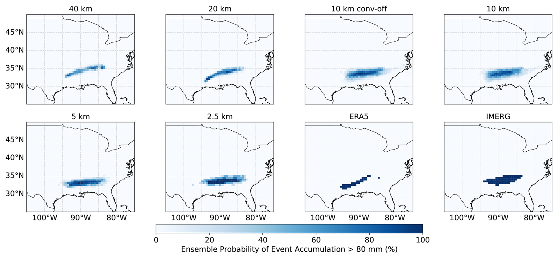
Figure A1 Probability of having an ensemble member exceeding 80 mm of precipitation over the entire event at each grid spacing. We shows the results for all ICON grid spacings considered as well as ERA5 and IMERG. The accumulated precipitation is computed between the 10 and 12 February.

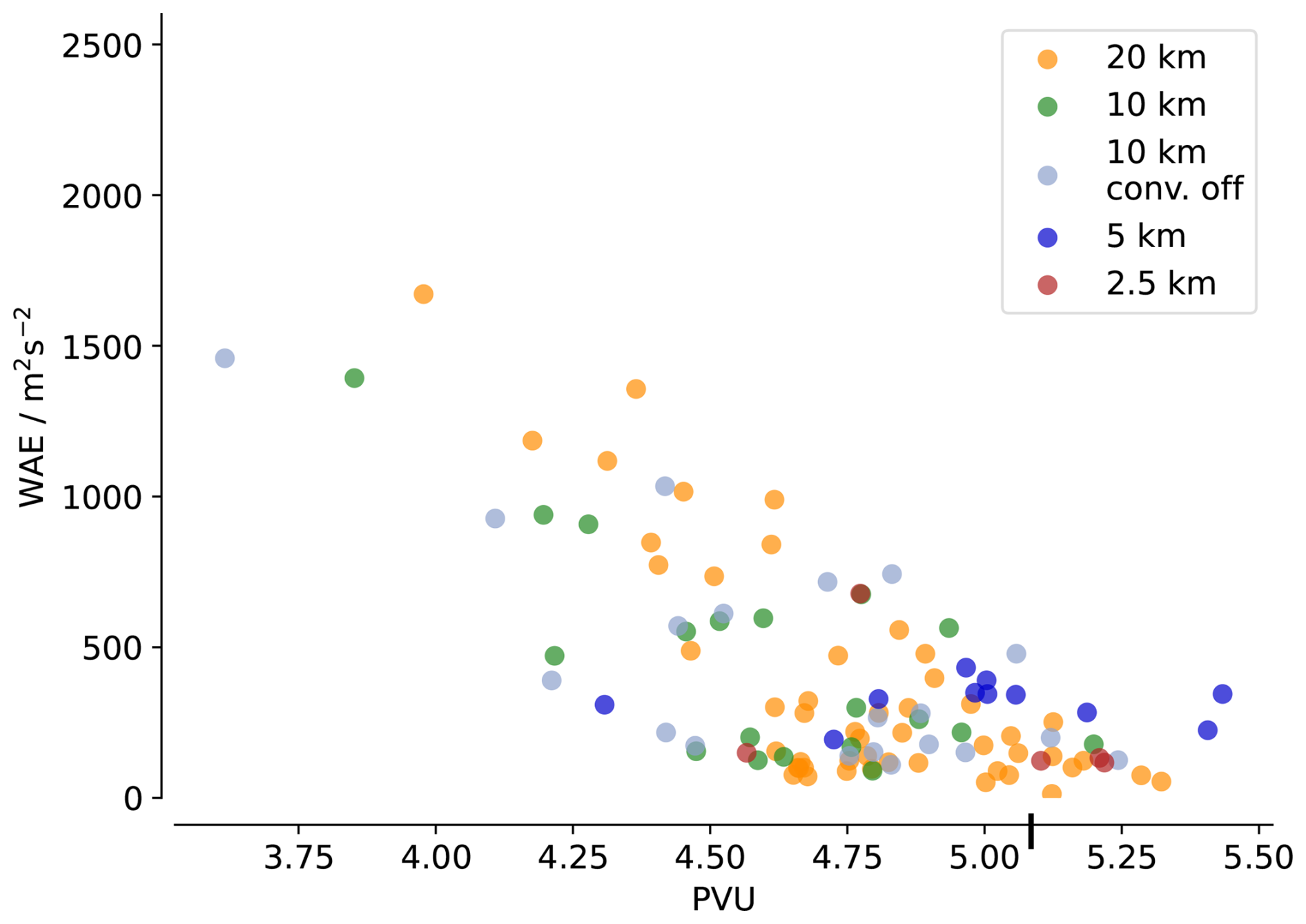
Figure A2 Correlation between the mean PVU at 250 hPa within the trough region (70 to 50° W and 40 to 55° N) on 12 February at 15:00 UTC versus mean WAE for each ensemble at each grid spacing. The vertical tick on the x-axis is the ERA5 mean PVU value as a reference.

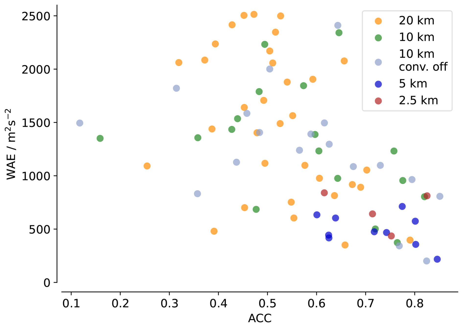
Figure A3 Correlation between the mean WAE at 250 hPa within the trough region (70 to 50° W and 40 to 55° N) on 12 February at 15:00 UTC versus the ACC on day 6 for each simulation at each grid spacing.

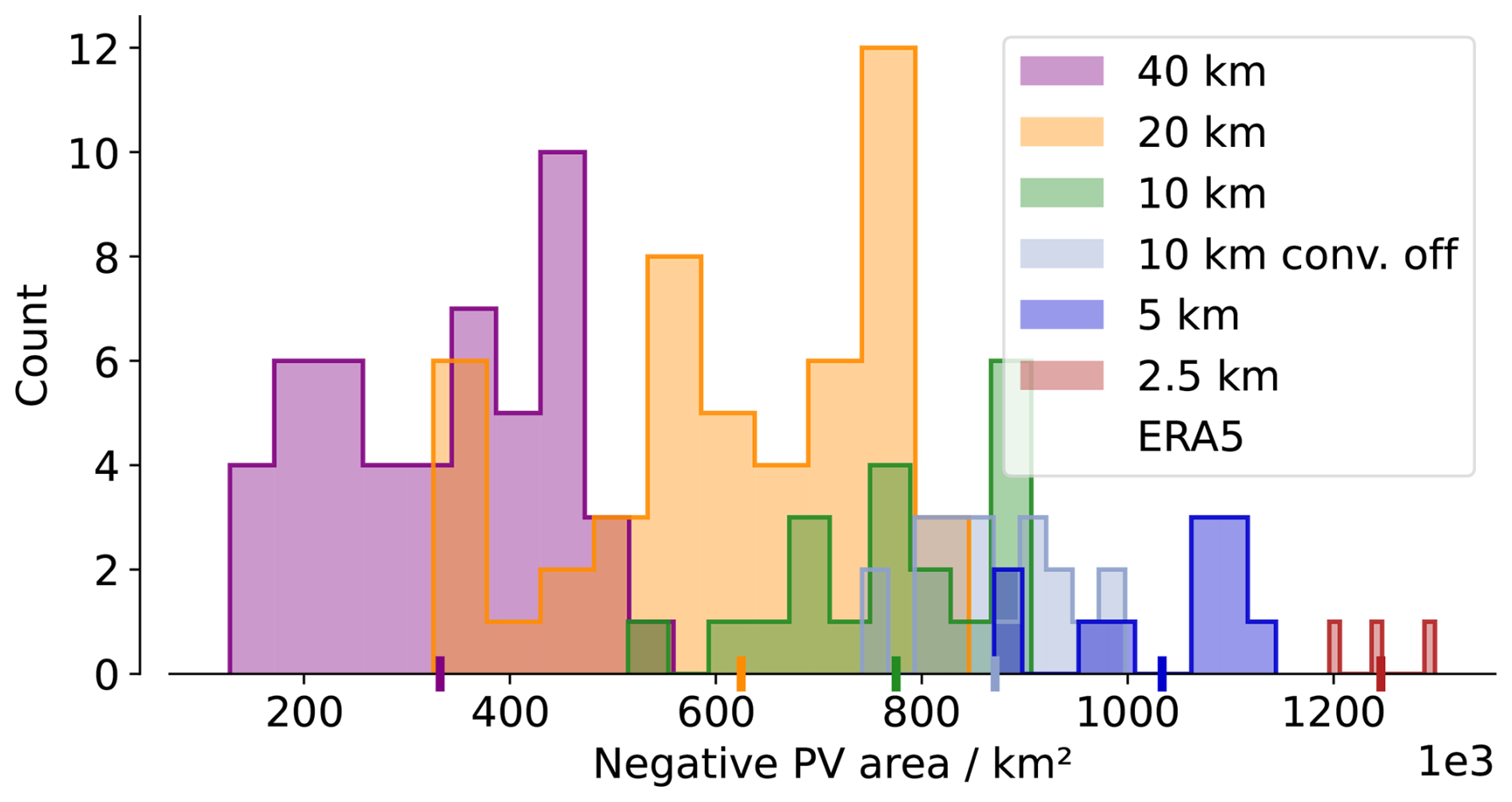
Figure A4 Similar as Fig. 3b, for the second case, with initialization on the 30 August and evaluation on the 2 September 15:00 UTC within (60 to 30° W, 35 to 60° N).

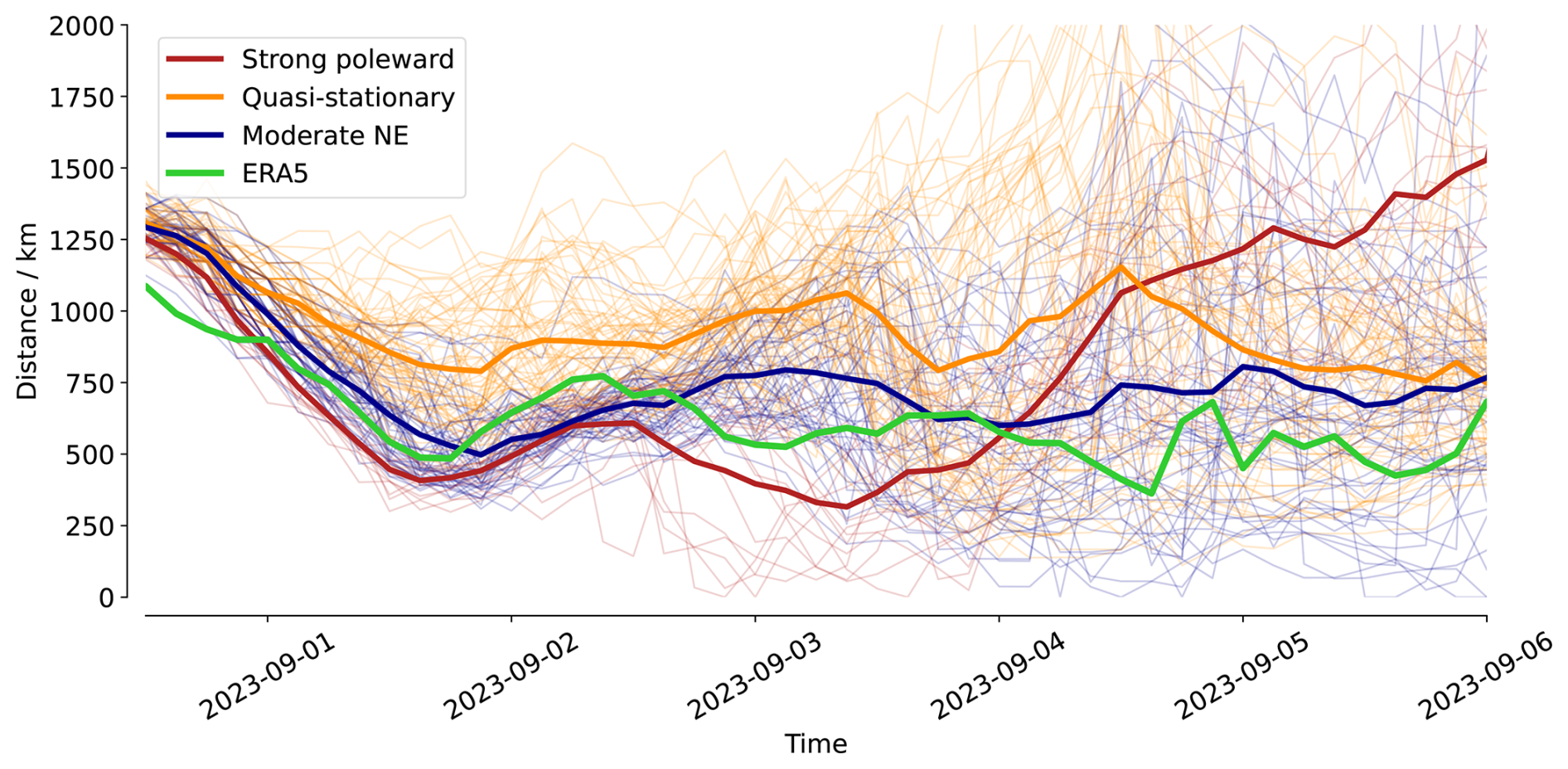
Figure A5 Distance between the cyclone and the jet stream for all ensemble members at all resolutions, colored depending on their clusters defined in Fig. 7. The thick lines show clusters means, and the green line shows the ERA5 reference.

Figure A6 Similar as Fig. 4b, for the WCBs of all ensembles at each grid spacing for the third case studied.