Relating extratropical atmospheric heat transport to cyclone life cycle characteristics and numbers in Southern Hemispheric winter

Outside the tropics, extratropical cyclones account for most of the poleward atmospheric heat transport, and extreme heat transport events are known to occur in their vicinity. Yet, it remains unclear how individual cyclones contribute to heat transport over the course of their lifetime and whether the seasonal heat transport – viewed from a zonally integrated standpoint – is determined by their number. This study adopts a cyclone-centered perspective to quantify in detail the relationship between poleward heat transport and the life cycle characteristics of extratropical cyclones in Southern Hemispheric winter. Specifically, objectively identified surface cyclone tracks derived from ERA5 data (1981–2021) are combined with a moist static energy (MSE) framework involving an eddy-mean decomposition of the meridional MSE flux.

It is found that the local transient eddy MSE flux maximizes during the cyclone intensification phase and is largest in the warm sector with a secondary maximum in the cold sector. A considerable fraction of the flux in the warm sector is located well equatorward of the cyclone and thus outside the cyclonic region identified by the tracking algorithm. This leads to a latitudinal shift between maxima in cyclone frequency and transient eddy MSE fluxes. To bridge the gap between zonally integrated MSE flux and contributions from individual cyclones, local vertically integrated transient eddy MSE flux events are attributed to cyclones based on spatial overlap with the identified cyclone area. Poleward of 50° S, the cyclones that become most intense are the ones that exhibit the largest zonally integrated cyclone-attributed MSE flux while the strongly intensifying cyclones dominate equatorward thereof. Although both of these sets of cyclones contribute disproportionally to the cyclone-attributed transient eddy MSE fluxes, the relationship between their seasonal number and the seasonal mean poleward transient eddy MSE flux is sensitive to the choice of the eddy-mean decomposition method. This result indicates that low wavenumber background flows mask the influence of cyclone intensities and intensification rates in the vertical, zonal, and seasonal integral. Notably, at 50° S the relationship between the overall cyclone number and total MSE flux shows a peak. Further research on the interplay between synoptic and planetary MSE fluxes in the vicinity of cyclones is needed to understand to which extent the cyclone number may be constrained by the global energy imbalance.

1 Introduction

The life cycle of an extratropical cyclone typically consists of an intensification phase followed by a weakening phase. A key characteristic of the cyclone life cycle is the rate of intensification, which is not only of scientific interest but also of societal relevance as rapidly intensifying cyclones can be related to particularly large economic impacts (e.g., storm “Lothar”; Wernli et al., 2002). It is well known that extratropical cyclones intensify in regions of large baroclinicity, i.e., where horizontal temperature gradients are large and static stability is relatively low (Lindzen and Farrell, 1980) – for instance in the Gulf Stream region, which exhibits a land-sea temperature contrast, or across the Antarctic sea ice edge. The mean baroclinicity thereby helps to understand why extratropical cyclones develop in localized geographic regions (called storm tracks). The intensification of individual storms can be further amplified by the release of latent heat during condensation (e.g., Booth et al., 2013; Büeler and Pfahl, 2017), which takes place in the ascent regions along the fronts or within the cyclone center (e.g., Attinger et al., 2019; Rüdisühli et al., 2020). Therefore, the strengthening of an individual extratropical cyclone can be described as baroclinic intensification modulated by diabatic heat release and an associated poleward heat transport. However, baroclinic theory falls short when it comes to explaining the number of storms that develops over a certain time span (e.g., a season) or how changes in the number of cyclones relate to changes in different life cycle characteristics, which also include the lifetimes and intensities. A small number of intense cyclones, for example, may erode as much baroclinicity as many weak cyclones (Sinclair and Catto, 2023).

According to baroclinic theory, cyclones intensify as long as there is a poleward transport of heat in their vicinity (Charney, 1947; Eady, 1949). These systems thus contribute to the poleward atmospheric heat transport which counteracts the radiative imbalance between the equator and the pole (Peixoto and Oort, 1992). Especially in the warm sector downstream of a cyclone, the poleward heat transport is not only linked to sensible heat but also the fraction of latent heat that is not immediately condensed. Thus, a convenient quantity to quantify the total atmospheric heat transport is the flux of moist static energy (MSE). MSE is the sum of latent and dry heat and potential energy.

The poleward flux of MSE occurs on different time-scales and length-scales. Therefore, the total flux is commonly decomposed into eddy and background flux contributions (e.g., Priestley, 1949; Marshall et al., 2014; Barpanda and Shaw, 2017). Traditionally, one then inspects the zonal integrals of the MSE fluxes. In such a zonal integral framework, the MSE flux related to the zonally averaged circulation represents the overturning circulation, which in the midlatitudes corresponds to the Ferrell cell that transports heat equatorward. Another considerable fraction of poleward MSE flux is associated with low-frequency planetary-scale waves, especially in the Northern Hemisphere (NH; Barpanda and Shaw, 2017; Stoll et al., 2023). The largest share of midlatitude MSE flux is, however, related to synoptic-scale eddies (e.g., Peixoto and Oort, 1992; Armour et al., 2019; Stoll et al., 2023). If the eddy-mean decomposition is adopted in the time dimension, this is often referred to as the “transient” eddy MSE flux (e.g., Messori and Czaja, 2015; Barpanda and Shaw, 2017). So far, most efforts to relate this transient eddy MSE flux to storm track dynamics have largely relied on zonally integrated MSE fluxes (Barpanda and Shaw, 2017; Shaw et al., 2018). The zonally integrated MSE flux, separated by spatial scale, has been investigated in the context of weather regimes (Lembo et al., 2022). Regardless of the chosen decomposition method, however, the contributions of (individual) cyclones to the zonally integrated MSE flux have not been systematically quantified. From analyses on the transport of latent heat, it is known that cyclones play a pivotal role for the total transport throughout the SH extratropics (Sinclair and Dacre, 2019) and into Antarctica (Tsukernik and Lynch, 2013). This motivates investigating to which degree extratropical cyclones modulate the total MSE flux in the zonal integral.

Previously, local (extreme) transient eddy MSE fluxes have been linked to the warm and cold sectors of midlatitude cyclones (Messori and Czaja, 2015; Messori et al., 2017). These MSE flux peaks typically form banded structures which, in some cases, follow the frontal zones near surface cyclones (Geen et al., 2016; Messori et al., 2017). These events majorly contribute to the zonally integrated transient eddy MSE flux (Messori and Czaja, 2013). In addition, days with enhanced zonally integrated transient eddy MSE fluxes have a disproportionate impact on the seasonal integral (Messori and Czaja, 2015) which suggests that local extreme events may significantly contribute to climatological zonally integrated flux. Conversely, it was found that local flux extremes arise from a constructive interference of synoptic and planetary waves in MSE and the meridional wind (Messori and Czaja, 2014). This indicates that transient eddy MSE fluxes in the vicinity of a cyclone might not solely be determined by its life cycle characteristics but also contain contributions from low-frequency background flows. Despite this extensive research on local MSE fluxes, a systematic analysis of when during the cyclone life cycle MSE fluxes maximize has not been performed. Consequently, it remains unclear which life cycle characteristic most strongly modulates the instantaneous zonally integrated transient eddy MSE flux and how much individual cyclones contribute to the seasonally integrated flux (Messori and Czaja, 2015) depending on their characteristics.

This study is further motivated by the modeled decrease in the number of cyclones under global warming. Most studies that investigate cyclone numbers within coupled climate simulations agree that the cyclone number in SH winter decreases in a warmer climate (König et al., 1993; Geng and Sugi, 2003; Lambert and Fyfe, 2006; Grieger et al., 2014; Chang, 2017; Priestley and Catto, 2022) whereas Chang et al. (2012) identified no robust decrease apart from the Atlantic sector. This response to warming is also underpinned by highly idealized atmosphere-only experiments (Sinclair et al., 2020; Schemm et al., 2022). A plausible explanation for this reduction could be that, as individual cyclones transport more latent heat because of the Clausius–Clapeyron relationship (Geen et al., 2016), fewer cyclones account for same amount of MSE flux (Zhang and Wang, 1997) that is required to counteract the equator-to-pole radiative energy imbalance. Yet, the total MSE flux does not remain constant under CO₂-forcing (as had been suggested by Boer, 1995) but exhibits a latitude-dependent response (Donohoe et al., 2020). Moreover, the change in MSE transported by individual cyclones likely also depends on the cyclone characteristics such as the intensity or spatial extent, which are projected to change as well (Dai and Nie, 2022; Priestley and Catto, 2022). Thus, how the partitioning of the total MSE flux onto extratropical cyclones changes under warming is non-trivial. Addressing the storm track response to climate forcing therefore necessitates a more profound understanding of the relationship between zonally integrated MSE fluxes and the number of cyclones under present climate conditions. To achieve this, it is inevitable to examine how MSE flux is locally related to extratropical cyclones in the first place.

The overarching goal of this study is to bridge the gap between the synoptic-scale cyclone and zonally integrated poleward heat transport perspectives under current climate conditions. We follow the assumption that the poleward MSE flux related to cyclones is described by the eddy component of a flux decomposition, and hereafter refer to this simply as the transient MSE flux (regardless of whether referring to a decomposition in time or space). To build a solid understanding of how transient MSE flux relates to cyclones, first the spatio-temporal relationship is explored locally and during the typical cyclone life cycle. Building on that, we inspect the contribution of individual cyclones to the zonally integrated transient MSE flux by introducing a feature-based approach to attribute transient MSE fluxes to individual cyclones. Finally, we examine the inter-annual variability of the seasonal cyclone number along with seasonal transient MSE fluxes. We focus on the SH storm track during the winter months June, July, and August (JJA). In contrast to the NH, the SH storm track is nearly circumpolar and therefore more zonally symmetric, which simplifies linking zonally integrated fluxes to cyclone characteristics. Moreover, winter is the season during which cyclone activity is maximum. The specific research questions thus are:

• How does the local transient MSE flux evolve during the life cycle of extratropical cyclones?

• How much of the zonally integrated transient MSE flux can be attributed to cyclones, and how do their contributions differ according to their key life cycle characteristics such as intensification rate, intensity, and lifetime?

• On a seasonal scale, how are (transient and total) MSE fluxes related to the number of cyclones at a given latitude band?

The methods applied in this study are detailed in Sect. 2. The evolution of transient MSE fluxes along cyclone life cycles, including spatial composites, is presented in Sect. 3. How cyclone characteristics influence the MSE flux of a cyclone in the zonal integral is shown and discussed in Sect. 4. The seasonal relationship between (transient) MSE flux and the number of cyclones is examined in Sect. 5. Finally, the results are summarized and discussed in a broader context in Sect. 6.

2 Methods

2.1 Reanalysis data

All computations of this study are based on the ERA5 reanalysis (Hersbach et al., 2020). The focus is on the winter season, i.e., JJA, in the SH during the years 1981 to 2021. All variables are obtained at 0.5° × 0.5° horizontal grid resolution. MSE fluxes are computed using six-hourly resolution and on 28 of the 37 available pressure levels spanning 1–1000 hPa.¹

2.2 Cyclone tracking

2.2.1 Automated cyclone tracking

Extratropical cyclones are objectively identified using the cyclone tracking algorithm developed by Wernli and Schwierz (2006), which was refined to improve the handling of splitting and merging events by Sprenger et al. (2017). Local minima in sea level pressure (SLP) are identified and followed over time which yields individual cyclone tracks. In a second step, a cyclone mask is defined as the area within the outermost closed SLP contour around a SLP minimum. Following Sprenger et al. (2017), the upper bound for the outermost closed contour is chosen to be 7500 km. The lifetime of a cyclone is defined as the number of time steps of its track starting at genesis and including lysis. The maximum intensity is defined as the minimum SLP along the track and the intensification rate as the change in SLP between two consecutive time steps. While cyclones are tracked using hourly SLP input, only six-hourly time steps are considered in the analysis to match the temporal resolution of the calculated MSE fluxes.

2.2.2 Track postprocessing

In this study, the goal is to focus on well-defined cyclone tracks that exhibit a clear intensification phase. This requires filtering out all of the objectively identified tracks that only weaken over time, i.e., for which the minimum SLP solely increases. For our track selection, we make use of the intensification metric proposed by Sanders and Gyakum (1980): for each track, the running finite difference in SLP over 24 h is normalized with $\frac{\sin \mathrm{60}\mathit{°}\text{S}}{\sin \mathit{\varphi }}$, where ϕ represents the latitude of the cyclone center averaged over the corresponding 24 h. The minimum of the resulting timeseries is multiplied with −1 and thereby defines the peak intensification rate of the cyclone. The multiplication with −1 is performed such that a positive value signifies that the cyclone undergoes intensification during its life cycle. This intensification rate is usually expressed in Bergeron. As a reference, 1 Bergeron corresponds to an change in minium SLP of −24 hPa d⁻¹ at 60° S. In short, we only consider tracks with intensification rate larger than 0 Bergeron. By design of the above metric, tracks shorter than 24 h are excluded. Moreover, we discard tracks with for which the minimum SLP remains above 990 hPa to remove spurious tracks in and around topography. Lastly, we filter out tracks that do not intensify poleward of 30° S, i.e., tropical cyclones without an extratropical transition.

Measuring the intensification rate in Bergeron is particularly important when investigating and comparing cyclones across an entire hemisphere. Likewise, when selecting cyclone subsets we define the intensity of a cyclone using SLP anomalies from local climatology (as in Cornér et al., 2025, for instance) rather than absolute SLP values. This correction is performed to circumvent a systematic bias arising from the climatological decrease in SLP towards the poles.

2.2.3 Cyclone-centered composites

To investigate the transient MSE fluxes associated with cyclones, cyclone-centered composites are computed at different stages of the cyclone life cycle. For the composites, atmospheric fields are regridded such that the cyclone center is located at (0,0) in cyclone-centered coordinates. Bilinear interpolation is used for all variables except precipitation, for which conservative remapping is applied. Importantly, we refrain from rotating along the direction of propagation (unlike, e.g., Catto et al., 2010) in order to preserve the distinction between meridional and zonal winds and MSE fluxes.

2.3 MSE fluxes

2.3.1 The general zonal mean heat budget of the atmosphere

The atmospheric heat transport is quantified by the flux of MSE. MSE is defined as $m=h+\mathrm{\Phi }$ where the first contribution is the thermal energy of the atmosphere $h=c_{p}T+Lq$ where c_p is the specific heat capacity, L is the latent heat of evaporation, T is temperature, q denotes specific humidity, and Φ is geopotential. In the vertical integral and zonal average (denoted with 〈⋅〉 and [⋅], respectively), the local atmospheric heat budget (as derived, for instance, in Trenberth, 1991) is written as

$$\begin{array}{}\text{(1)}& {\partial }_t\langle \left[h\right]\rangle =\left[F_{\text{TOA}}-F_{\text{S}}\right]-{\partial }_y\langle \left[vm\right]\rangle .\end{array}$$

F_TOA and F_S represent the net energy flux at the top of atmosphere (TOA) and surface, respectively, and v denotes meridional wind (Neelin and Held, 1987; Barpanda and Shaw, 2017). F_TOA is comprised of only radiative fluxes whereas F_S includes both radiative fluxes at the surface and turbulent fluxes. The temporal change in the storage h is thus simply determined by the convergence of MSE flux and the net energy input at the surface and TOA.

The meridional divergence is computed as ${\partial }_y(\cdot )\equiv {\partial }_{\mathit{\varphi }}\mathit{\left\{}\cos \mathit{\varphi }\right(\cdot \left)\mathit{\right\}}/\left(a\cos \mathit{\varphi }\right)$ where a is the radius of Earth. The vertical integral is mass-weighted ($\langle \cdot \rangle \equiv \frac{\mathrm{1}}{g}{\int }_{\mathrm{0}}^{\stackrel{\mathrm{‾}}{p_{\text{S}}}}(\cdot )\mathrm{d}p$) and computed from the TOA to the climatological mean surface pressure $\stackrel{\mathrm{‾}}{p_{\text{S}}}$ (Boer and Sargent, 1985). This formulation neglects kinetic energy and latent heat related to the liquid-ice transition (Mayer et al., 2024) and defines fluxes relative to a fixed mass of atmosphere following Cox et al. (2024b).

2.3.2 Decomposition of the MSE fluxes

We further decompose the MSE flux into eddy and mean components. Eddy fluxes are defined via deviations from a background mean state and are traditionally thought to be related to synoptic weather systems (e.g., Kaspi and Schneider, 2013; Barpanda and Shaw, 2017). One established approach defines the background state using monthly means, such that the monthly mean flux reads

$$\begin{array}{}\text{(2)}& \left[\stackrel{\mathrm{‾}}{vm}\right]=\left[\stackrel{\mathrm{‾}}{v^{\prime }{m}^{\prime }}\right]+\left[{\stackrel{\mathrm{‾}}{v}}^{*}{\stackrel{\mathrm{‾}}{m}}^{*}\right]+\left[\stackrel{\mathrm{‾}}{v}\right]\left[\stackrel{\mathrm{‾}}{m}\right]\end{array}$$

with dashes and asterisks signifying anomalies from the monthly $\stackrel{\mathrm{‾}}{(\cdot )}$ and zonal averages, respectively (Priestley, 1949; Peixoto and Oort, 1992). Following Barpanda and Shaw (2017), the first two terms on the right hand side represent fluxes by transient and (temporally) stationary eddies, respectively, whereas the third term corresponds to the meridional overturning circulation.

To investigate the total MSE flux, we perform a correction to account for mass conservation, which is not guaranteed in ERA5 (e.g., Mayer et al., 2021). In the zonal mean, mass-conservation corresponds to 〈[v]〉 = 0 when calculating MSE flux with respect to a time-independent atmospheric mass. We thus adopt the approach introduced by Marshall et al. (2014) and subtract vertical averages of [m] and [v] before computing the overturning circulation. Thereby, the MSE flux that is related to a net mass flux, which can be unrealistically large (Cox et al., 2023), is removed.

2.3.3 Sensitivity regarding the decomposition

Defining transient eddies as deviations from monthly mean data introduces discontinuities at the end of each month. We explore the sensitivities of the results using two additional definitions of transient eddies: (i) high-pass filtering (e.g., Hoskins et al., 1983; Schemm and Rivière, 2019; Franzke and Harnik, 2023) with a cut-off frequency of 10 d and; (ii) defining eddies as anomalies from instantaneous zonal means (Cox et al., 2024b). This eddy flux thus depends on the atmospheric state up- and downstream at the same latitude. In contrast, the eddy flux in the other two methods depends on the characteristics of the time series of the data at the same location.

Throughout the manuscript, we use superscripts to indicate anomalies: A prime $(\cdot {)}^{\prime }$ for deviations from a temporal mean (referred to as `transient' anomaly), and $(\cdot {)}^{*}$ for deviations from the zonal mean. The subscript denotes the decomposition method: MA indicates monthly anomalies, HP refers to high-pass filtering, and ZA indicates zonal anomalies. Thus, in sensitivity tests we compare $v^{\prime }{m}_{\mathrm{MA}}^{\prime }$ to $v^{\prime }{m}_{\mathrm{HP}}^{\prime }$ and $v^{*}{m}_{\mathrm{ZA}}^{*}$. In the following sections, regardless of the decomposition all of these three MSE fluxes are referred to as “transient” and the prefix “eddy” is omitted for brevity. A complete list of the used mathematical symbols is provided in Sect. S1 in the Supplement.

2.4 Attributing MSE fluxes to cyclones

This section describes how local transient MSE fluxes are attributed to individual cyclones. The simplest approach is to spatially integrate the MSE fluxes over the SLP-based cyclone mask at each timestep. However, there is an important issue with this approach. In the climatology the maximum transient MSE flux is located equatorward of the maximum in surface cyclone frequencies (Fig. 1a). This is similar to the relationship between surface cyclones and eddy kinetic energy (e.g., Shaw et al., 2016). Schemm et al. (2018) argue that this latitudinal offset occurs because eddy fluxes peak during the rapid intensification phase of extratropical cyclones, whereas cyclone detection frequencies peak in regions where cyclones have evolved into mature, slowly propagating systems. This latitudinal offset is also evident in the zonal mean (Fig. 1b): in the SH, transient MSE flux peaks at 6 PW around 45° S, while the zonally integrated cyclone frequency reaches up to 12 % near 62° S. Thus, most of the transient MSE fluxes are expected to be excluded when spatially integrating fluxes only within the SLP-based cyclone masks.

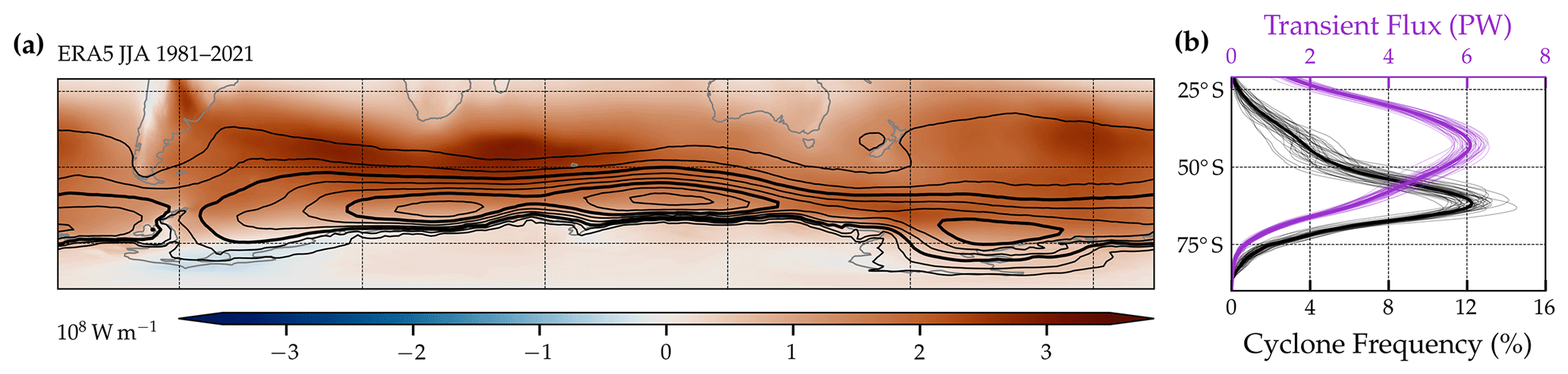
Figure 1 Climatologies of transient MSE fluxes and cyclone frequencies during SH winter (JJA). (a) Vertically integrated and seasonally averaged transient MSE fluxes, $\langle {\stackrel{\mathrm{‾}}{v^{\prime }{m}^{\prime }}}_{\mathrm{MA}}\rangle$, (shading) are shown along with the cyclone mask frequency (black contours in steps of 5 % starting at 5 % with 15 % and 30 % highlighted in thicker contours). (b) Zonally integrated transient MSE fluxes, $\langle \left[{\stackrel{\mathrm{‾}}{v^{\prime }{m}^{\prime }}}_{\mathrm{MA}}\right]\rangle$, (purple) and zonal mean cyclone frequencies (black) for individual seasons (thin lines) and the climatology thereof (solid lines). MSE fluxes are shown positive poleward. Note that the cyclone frequency in panel (b) is multiplied with the cosine of latitude for consistency.

To overcome this latitudinal gap between the two storm track metrics, a flux attribution method is introduced that identifies coherent MSE flux features and connects them to cyclones if they spatially overlap with SLP-based cyclone masks. The transient MSE flux features in this work are identified using a percentile threshold (similarly to studies tracking atmospheric rivers, Shields et al., 2018). To account for the high latitudinal and monthly variability of MSE, the threshold is chosen to be latitude- and time-dependent. More specifically, the percentile is drawn from all values of a latitude band at the same time step of each year, (see Fig. S1 in the Supplement). Thus, it is computed from 29 520 values (360° $/$ gridspacing × the number of years as illustrated in Fig. S2). Given a percentile rank 0.5 < p < 1, the vertically integrated transient flux $\langle v^{\prime }{m}_{\mathrm{MA}}^{\prime }\rangle$ is masked twice using the flux thresholds corresponding to p and 1−p for northward and southward fluxes, respectively.

Areas in which these flux thresholds are exceeded are defined as MSE flux features. Such features are identified and labeled using TempestExtremes v2.1 (Ullrich et al., 2021). Small features (4.9 × 10⁴ km² or approximately 1° × 1°), which are located predominantly in the tropics and subtropics, are discarded. The remaining features (describing both poleward and equatorward flux) are attributed to individual cyclone tracks if they spatially overlap with the SLP-based cyclone masks (filled orange and blue patches in Fig. 2). This is done at every timestep separately as the MSE flux features are not tracked (or “stitched” in the language of the identification tool) over time. MSE flux features that do not overlap with cyclone masks are labeled as “other MSE fluxes” (orange and blue contours in Fig. 2). If a flux mask overlaps with multiple cyclones, the cyclone with the lowest center SLP is chosen. Randomly selecting between the overlapping cyclones was also tested, but had no qualitative effect on the results. Note that given the percentile rank p, the fraction of grid points attributed to cyclones is not exactly $\mathrm{2}\cdot (\mathrm{1}-p)$ (“northward” plus “equatorward” areas) but less because on the one hand, small features are filtered out, and, on the other hand, not all of the remaining features are attributed to cyclones. Due to the relative simplicity of the attribution method, sensitivity analyses boil down to the choice of p and the flux decomposition method. While the results in Sects. 4 and 5 are for p = 0.9, p = 0.8 and p = 0.95 were also tested. The percentile generally determines the width of the attributed features. The location of these features in turn differs depending on the decomposition method (Fig. S2).

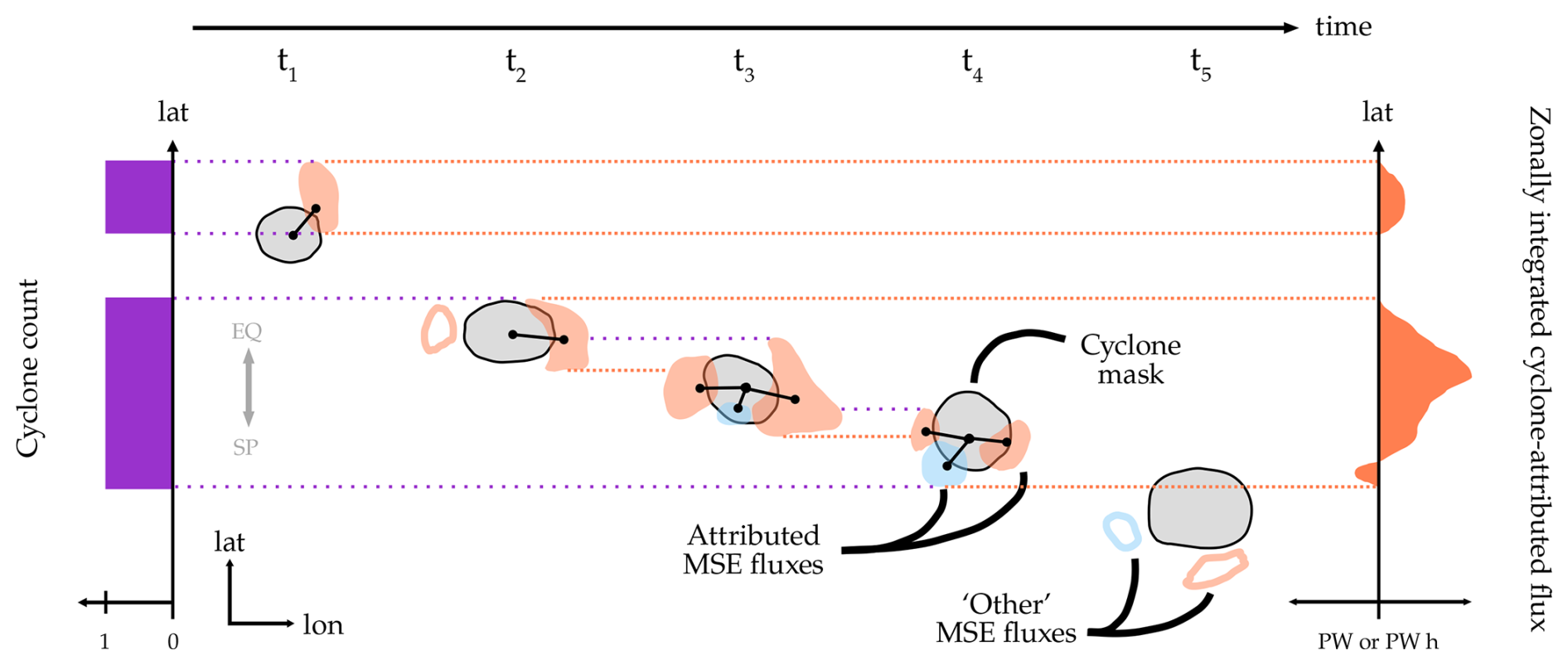
Figure 2 The attribution of transient MSE flux to surface cyclones exemplified for a cyclone that lasts for five six-hourly time steps. The cyclone mask is indicated with grey patches and the attributed poleward and equatorward transient MSE flux features with orange and blue shading, respectively. Other MSE fluxes that are not spatially overlapping are shown with orange and blue contours. In the zonal integral, cyclone-attributed transient MSE fluxes are expressed in PW h if accumulated or in PW if averaged over the cyclone lifetime (orange curve). The latitudinal extent used for counting is then determined by the latitudes at which the attributed fluxes during its lifetime are non-zero. At any latitude band, a cyclone is therefore counted either once or zero times (purple bars). A grey arrow serves orientational purposes.

2.5 Defining seasonal cyclone numbers using the cyclone-attributed MSE fluxes

In the zonally integrated heat budget, the MSE flux attributed to a cyclone is simply the zonal integral of the flux within the attributed MSE flux features (orange curve in Fig. 2). To define the cyclone number at each latitude, each cyclone is counted once towards all latitude bands where its attributed MSE flux is different from zero during its lifetime (purple bars in Fig. 2). Thus, the seasonal number of cyclones at a given latitude corresponds to the cyclones that have attributed transient MSE flux at this latitude, whereas the latitudes of their corresponding life cycle characteristics, such as the latitude at the time of maximum intensification, may be different.

The seasonal sets of strongly intensifying cyclones are then determined using climatological thresholds: cyclones are considered “strongly” intensifying if their intensification rate lies above the 75th percentile determined from the climatological set of all cyclones passing that latitude. If the 75th percentile of cyclone intensification based on all SH JJA cyclones is, for instance, 1 Bergeron, then this threshold defines the number of strongly intensifying cyclones in every season. Thus, their number is not simply 25 % of the seasonal number if that year has more or less strongly intensifying storms than the climatology. Choosing the 75th percentile (instead of the 90th, for instance) is found to be an adequate compromise between selecting only the strongest cyclones and including a large enough number of cyclones to counteract the event-to-event variability (see discussion in Sect. S4). If the intensification rate lies within the inter-quartile range or below, cyclones are denoted “moderately” or “weakly” intensifying, respectively. The classification of cyclones as “strong”, “moderate', and “weak” works analogously for intensity.

These methods enable us to study the relationship between various extratropical cyclone life cycle characteristics and MSE fluxes. They also allow us to analyze the fractional contribution of cyclone-related MSE flux to the zonally integrated poleward MSE flux and the relationship between cyclone the zonally integrated flux and cyclone number and intensity. By defining the number of cyclones as where they contribute to MSE flux we can study the linkage between cyclone numbers and atmospheric heat transport in a consistent way.

3 Local transient MSE fluxes in the vicinity of extratropical cyclones

First, it is investigated how the local transient MSE fluxes ($v^{\prime }{m}_{\mathrm{MA}}^{\prime }$) evolve during the extratropical cyclone life cycle and where they maximize relative to the cyclone center.

3.1 Temporal evolution of transient MSE flux during the life cycle of extratropical cyclones

To compare extratropical cyclones life cycles of different durations the transient MSE flux is interpolated to a normalized cyclone life cycle (e.g., Rudeva and Gulev, 2007; Schemm et al., 2018). Following previous studies, cyclone tracks are split into an intensification and a weakening phase and tracks with less than two time steps in each phase are removed from the analysis. The maximum transient MSE flux at 850 hPa within a 7.5° radius around the cyclone center is interpolated to the normalized life cycle using cubic spline interpolation (Fritsch and Carlson, 1980; Schemm et al., 2018).

Considering all SH cyclones, $v^{\prime }{m}_{\mathrm{MA}}^{\prime }$ peaks before mature stage and declines afterwards (black dashed line in Fig. 3). The peak flux during intensification is, on average, around 50 % larger than during the weakening phase. This evolution is broadly consistent with the baroclinic life cycle, in which transient eddy heat flux peaks as baroclinicity is eroded, before intensification terminates (Novak et al., 2015). Using larger attribution radii does not qualitatively affect this result, but it increases the proportion of flux attributed to a cyclone that, upon visual inspection, would be attributed to a nearby cyclone. For the 25 % most strongly intensifying cyclones, the peak of MSE flux during genesis is exaggerated with a median flux of almost 50 % larger during the intensification phase compared to all cyclones (blue line in Fig. 3). During the weakening phase, in turn, the fluxes near these cyclones decline markedly and become comparable to those observed for all cyclones. For the 25 % least rapidly intensifying cyclones (red line), the nearby fluxes remain at similarly low values even during the intensification phase. This highlights the close relationship between transient MSE flux and the intensity of baroclinic intensification. The following spatial analyses will thus focus entirely on the intensification phase and the most strongly intensifying cyclones.

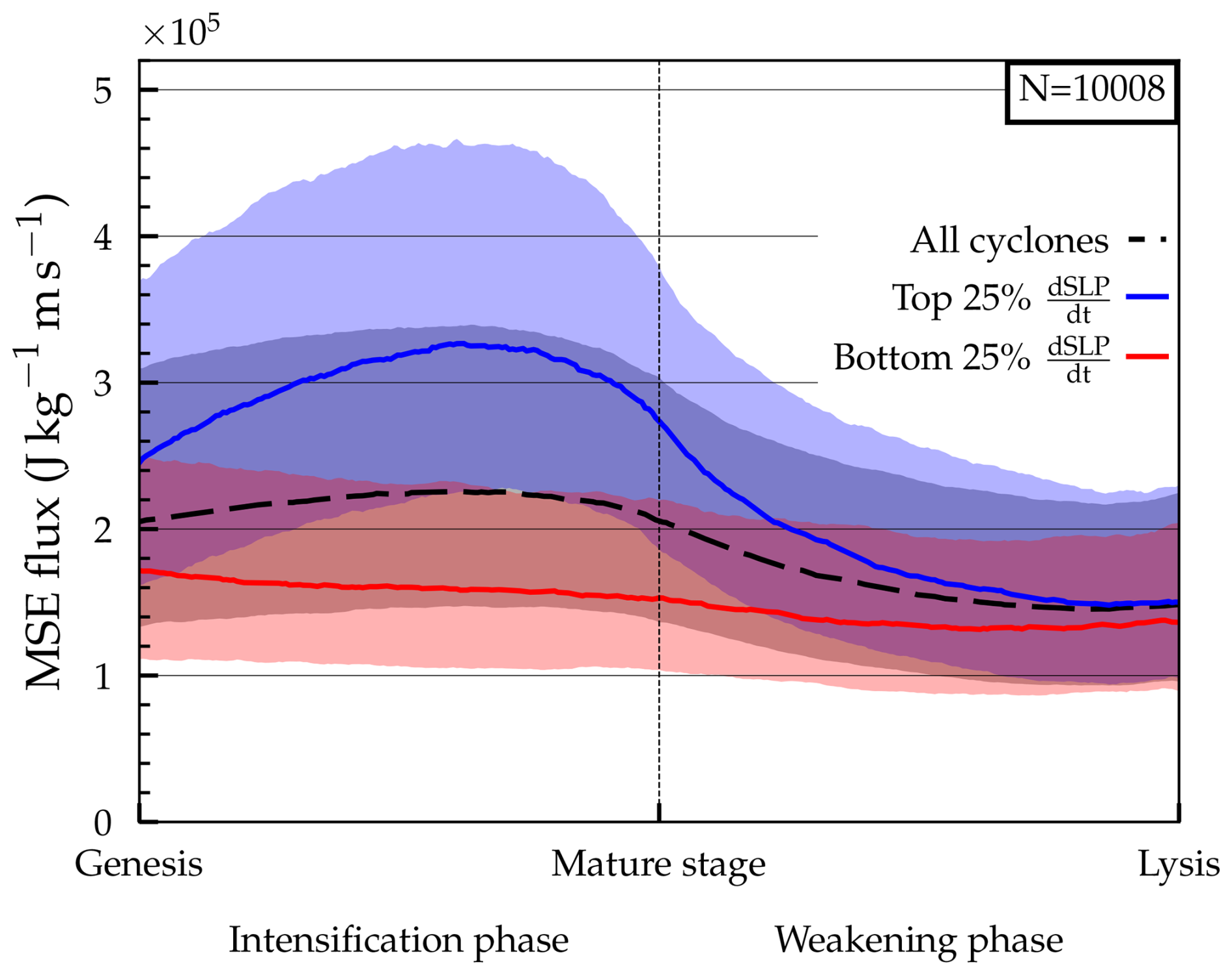
Figure 3 Maximum near-cyclone transient MSE flux, $v^{\prime }{m}_{\mathrm{MA}}^{\prime }$, at 850 hPa for all (black), the 25 % most strongly intensifying cyclones (blue), and the 25 % least strongly intensifying cyclones (red) during the normalized cyclone life cycle. The search radius is 7.5°. Median and interquartile range are shown in solid lines and shading, respectively. Genesis and lysis correspond to the first and last time steps of the track, respectively, while the mature stage is defined as the time of minimum central SLP. The number of all SH cyclones is included in the upper right.

3.2 Spatial relation of transient MSE fluxes and cyclones

The spatial distribution of MSE fluxes around the cyclone center is studied using cyclone-centered composites. Recall that in the SH, cyclonic flow is clockwise and that poleward flux is chosen positive. Also, both the poleward transport of anomalously warm moist as well as the equatorward transport of anomalously cool and dry air result in a positive poleward MSE. Thus the warm and cold sectors both show up as positive MSE fluxes in the composites.

The composite based on all cyclones indicates a maximum in poleward $v^{\prime }{m}_{\mathrm{MA}}^{\prime }$ at the 850 hPa level in the warm sector of the cyclone center during all three key stages of the cyclone life cycle (Fig. 4a–c). The MSE flux is generally larger on the equatorward side of the cyclone center. This is consistent with previous findings that MSE flux is bound by the frontal zones (compare, for instance, with the 990 hPa lines in Fig. 4; Geen et al., 2016; Messori et al., 2017) which in the SH frequently extend to 20–40° S which is well equatorward of the cyclone centers (Schemm et al., 2015; Rudeva et al., 2019). Closer inspection of the peak at genesis indicates that, in some cases, the flux is associated with a cold front accompanying a mature cyclone further downstream (not shown). This suggests that some cases are secondary cyclogenesis events, when a cyclone intensifies on the pre-existing front of a mature system (Schemm and Sprenger, 2015). During mature stage, the location of the maximum poleward flux is located further downstream in the warm sector relative to its position at genesis, when it is located closer to the cold front. In addition, a negative flux upstream of the cyclone center emerges at rlon = −1°, rlat = 0° in the local coordinates (light blue patch in Fig. 4c). While the warm sector features a local flux peak during all life cycle stages, the cold sector displays a well-marked positive flux signal in the composites only at the mature stage (Fig. 4c).

In vertical west-to-east cross-sections through the cyclone center, the pronounced warm sector flux extends up to roughly 300 hPa during all stages and reaches its maximum at around 900 hPa (Fig. 4d–f). This signal is the footprint of the ascending warm and moist airstream known as warm conveyor belt, which was also identified by centering around 850 hPa MSE flux extremes instead of cyclone centers (Messori and Czaja, 2015). The aforementioned negative flux located near the cyclone center extends up to around 700 hPa, while around 500 hPa a second negative signal downstream of the center appears (Fig. 4f). All of the flux signals discussed here are significantly different from climatology (see Sect. S3, Fig. S3).

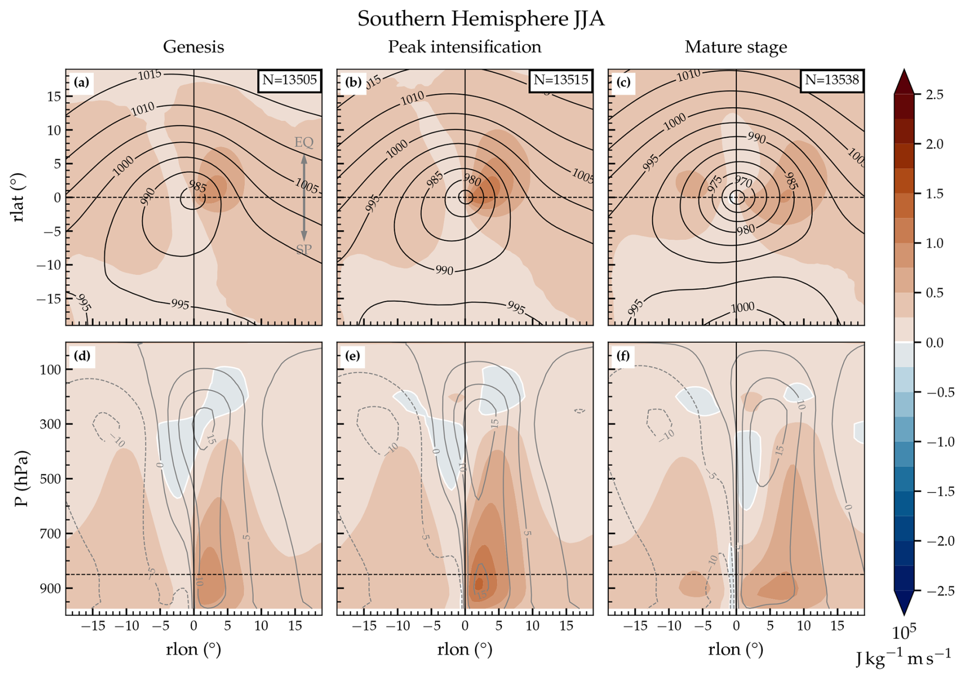
Figure 4 Cyclone-centered meridional transient MSE flux, $v^{\prime }{m}_{\mathrm{MA}}^{\prime }$, composited for different stages during the cyclone life cycle. Horizontal maps are shown for fluxes (colors) at 850 hPa for (a) genesis, (b) time of peak intensification, and (c) mature stage. Black contours indicate composite mean SLP in hPa. In panels (d)–(f), the west-to-east cross-sections through rlat = 0 correspond to the same stages as above. Grey lines depict meridional wind velocities (v^′) in m s⁻¹ (positive poleward). Horizontal dashed black lines represent the intersection of the corresponding vertical and horizontal panels. Furthermore, the number of cyclones in the composites are included in the upper right in panels (a)–(c). A grey arrow is included for better orientation indicating directions of equator (EQ) and South Pole (SP).

To briefly shed some light on the negative flux anomalies, consideration is given to composite mean meridional winds (grey lines in Fig. 4d–f). Overall, the wind anomalies tilt westward with height during intensification and become more barotropic at mature stage² which agrees with baroclinic theory (Eady, 1949; Thorncroft et al., 1993). For the mature stage, the wind field suggests that the mid-level negative flux signal at the 500 hPa level results from cold air moving poleward (Fig. 4f) and that the low-level equatorward flux represents warm and moist air flowing equatorward along the bent-back extension of the warm front (Shapiro and Keyser, 1990). The latter signal does not emerge when centering on flux extremes (Messori and Czaja, 2015).

The composite analysis confirms the above finding based on normalized tracks that meridional transient MSE fluxes near cyclones are, on average, largest during the intensification phase. Likewise, from a spatial composite perspective, the flux of the 25 % most strongly intensifying cyclones is roughly 50 % larger in the cold sector and up to 80 % larger in the warm sector compared to all cyclones (cf. Figs. 5a to 4b at 850 hPa). Strongly intensifying cyclones feature negative fluxes at 300 hPa downstream of the center, which can be related to the anticyclonic return flow of the warm conveyor belt and which are less prominent in the composites of all SH cyclones (compare Fig. 5c and Fig. 4e).

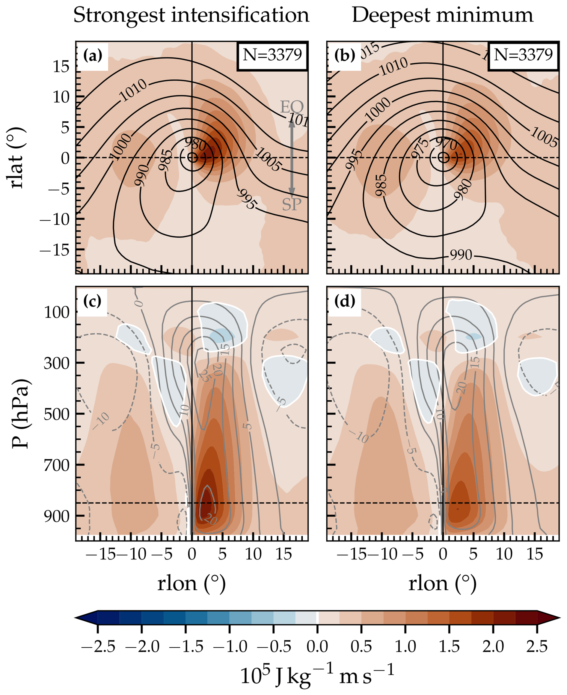
Figure 5 Cyclone-centered transient MSE flux at 850 hPa composited during time of peak intensification for (a) the 25 % most strongly intensifying cyclones and (b) the 25 % most intense cyclones at mature stage. Black contours indicate composite mean SLP in hPa. (c, d) The corresponding west-to-east cross-sections as in Fig. 4. Grey lines depict meridional wind velocities (v^′) in m s⁻¹ (positive poleward). Horizontal dashed black lines represent the intersection of the corresponding vertical and horizontal panels. Furthermore, the numbers of cyclones in the composites are included in panels (a) and (c). A grey arrow is included for better orientation indicating directions of equator (EQ) and South Pole (SP).

These conclusions remain unchanged when the most intense cyclones are considered instead of those that intensify most strongly. At the time of peak intensification, the warm sector peak is slightly reduced while the MSE flux in the cold sector is more spatially extended (Fig. 5b, d). This is in line with a larger cyclone size as estimated by the area outlined by the outermost closed SLP contour in the composites. Consistently with earlier studies, the most intense cyclones typically cover wider areas (Rudeva and Gulev, 2007) and are not necessarily the cyclones that intensify most rapidly.

3.3 Latitudinal variations of dry and latent heat flux contributions to the MSE flux

The asymmetry in the MSE flux between the cold and warm sectors is strongly related to the presence of moisture in the warm sector. The latitudinal distribution of specific humidity implies that also the contribution of latent heat flux to the MSE flux varies with latitude. To explore the dependency of the relative contributions by dry and latent heat flux on latitude, the top 25 % of cyclones with the strongest intensification are sorted into 10° latitude bands according to their center latitude at peak intensification.

Both MSE and latent heat flux decrease for cyclones closer to the pole (Fig. 6). The maximum of $v^{\prime }L{q}_{\mathrm{MA}}^{\prime }$, which is confined to the warm sector, largely overlaps with six-hourly accumulated precipitation (black contours in Fig. 6d, e). The relative contribution of $v^{\prime }L{q}_{\mathrm{MA}}^{\prime }$ reduces for cyclones propagating closer to the pole as expected due to the Clausius–Clapeyron relationship (black contours in Fig. 6a–c). As a result, the contrast between fluxes in the warm and cold sectors is strongly reduced for cyclones intensifying within 60–70° S (Fig. 6c). This points to a larger relative importance of cold air outbreaks to the heat budget towards higher latitudes (Messori et al., 2017).

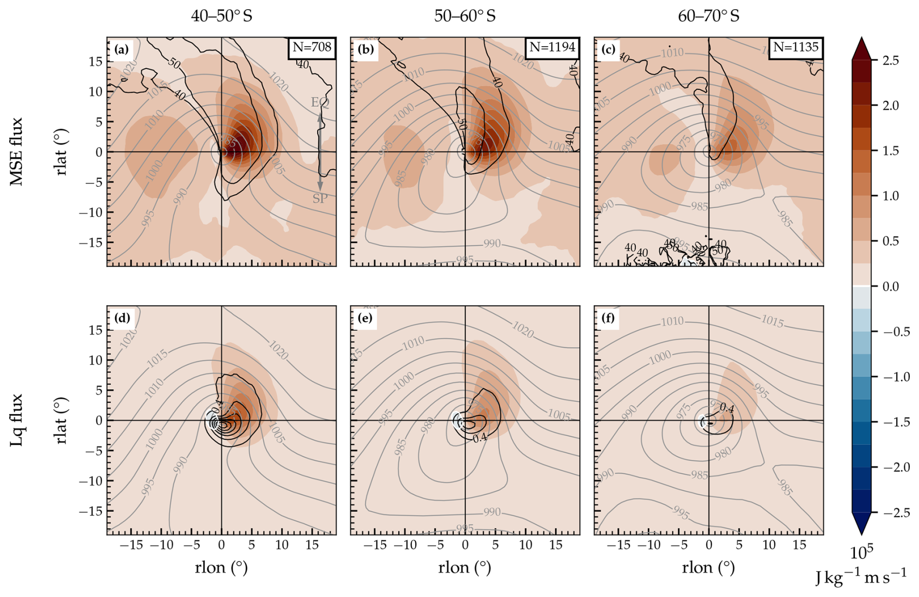
Figure 6 Cyclone-centered transient MSE flux, $v^{\prime }{m}_{\mathrm{MA}}^{\prime }$, at 850 hPa composited during time of peak intensification for the 25 % most strongly intensifying cyclones with center within (a) 40–50° S, (b) 50–60° S, and (c) 60–70° S. Shading in panels (d)–(f) indicates the latent heat flux, $v^{\prime }L{q}_{\mathrm{MA}}^{\prime }$. Regions where latent heat flux makes up for 40 % and 50 % of the MSE flux are outlined with black contours in panels (a)–(c). Black lines in panels (d)–(f) depict precipitation in steps of 0.4 mm h⁻¹. Grey contours indicate composite mean SLP in hPa. The number of cyclones in the composites are included in panels (a)–(c). A grey arrow is included for better orientation indicating the directions of the equator (EQ) and South Pole (SP).

We note that the dominance of warm sector MSE fluxes over cold sector fluxes may be amplified due to the nature of the composite approach. During the intensification phase, the cold front is usually located close to the center. Since MSE fluxes are large along the cold front, compositing by the cyclone center implies a tendency to center next to areas of pronounced warm sector fluxes. During the life cycle, the warm sector then narrows as the cold front catches up with the warm front (Shapiro and Keyser, 1990) such that the fluxes in the warm sector are spatially confined and always relatively close to the center. As the cold sector is not similarly constrained upstream, the distance from the cyclone center to the peak cold sector MSE flux is thought to be more variable. This would lead to cold sector MSE flux peaks being more smeared out in the composite than those from the warm sector.

Overall, the cyclone-centered perspective confirms and expands on previous findings on (low-level) transient MSE flux extremes (Messori and Czaja, 2015; Geen et al., 2016; Messori et al., 2017). As the following sections discuss vertically integrated MSE fluxes, it is worth pointing out that the findings regarding the horizontal structure of transient MSE fluxes also apply to vertically integrated fluxes (and fluxes calculated using different decompositions, see Sect. S3).

4 Cyclone-attributed MSE fluxes in the zonal integral

The goal of this section is to understand the contribution of cyclones to the zonal integrated transient MSE flux, $\langle \left[v^{\prime }{m}_{\mathrm{MA}}^{\prime }\right]\rangle$, which is a central term in the zonally and vertically integrated heat budget (Eq. 1). As Messori and Czaja (2015) showed that zonally integrated MSE flux extremes are driven by coexisting warm and cold sectors, it is deemed plausible that cyclones account for a considerable fraction of MSE flux in the zonal integral as well. Having found that the intensification rate strongly influences the local MSE flux, we further aim to quantify to what extent the different life cycle characteristics – especially the intensification rate, maximum intensity, and lifetime – modulate the zonally integrated MSE flux. As the previous composites are only snapshots during the life cycle, the guiding question is whether the intensification rate also influences the zonally integrated MSE flux integrated over the entire life cycle, or whether the maximum intensity or lifetime matter more.

Answering this questions requires computing MSE flux contributions of individual cyclones to the zonal integral. As suggested by Figs. 4–6, MSE flux frequently occurs outside of the SLP-based cyclone masks, which is also the case in the vertical integral (Fig. S4). Thus, in this section we make use of the newly introduced MSE flux attribution method.

4.1 Contribution of cyclone-attributed MSE flux to the zonal budget

The zonal integral of the seasonal mean cyclone-attributed transient MSE flux, denoted as $\langle \left[{\stackrel{\mathrm{‾}}{v^{\prime }{m}^{\prime }}}_{\mathrm{MA}}^{\mathrm{cycl}}\right]\rangle$, amounts to 1.65 PW at around 50° S (orange solid line in Fig. 7a).³ Thus, around 30 % of the overall transient MSE flux is attributed to cyclones (Fig. 7b), while the rest is attributed as non-cyclone related MSE flux. The correlation between the seasonal mean of the zonally integrated MSE flux and the cyclone-attributed transient MSE flux ranges from 0.5 around 40° S to 0.75 poleward of 55° S (orange line in Fig. 7c). The correlation is calculated assuming that the winter seasons are independent of each other. Due to the presence of other dynamical features, for example anticyclones, and the degrees of freedom when attributing MSE flux to cyclone masks, which are discussed in Sect. 2.4, one must not expect 100 % flux coverage or perfect correlation.

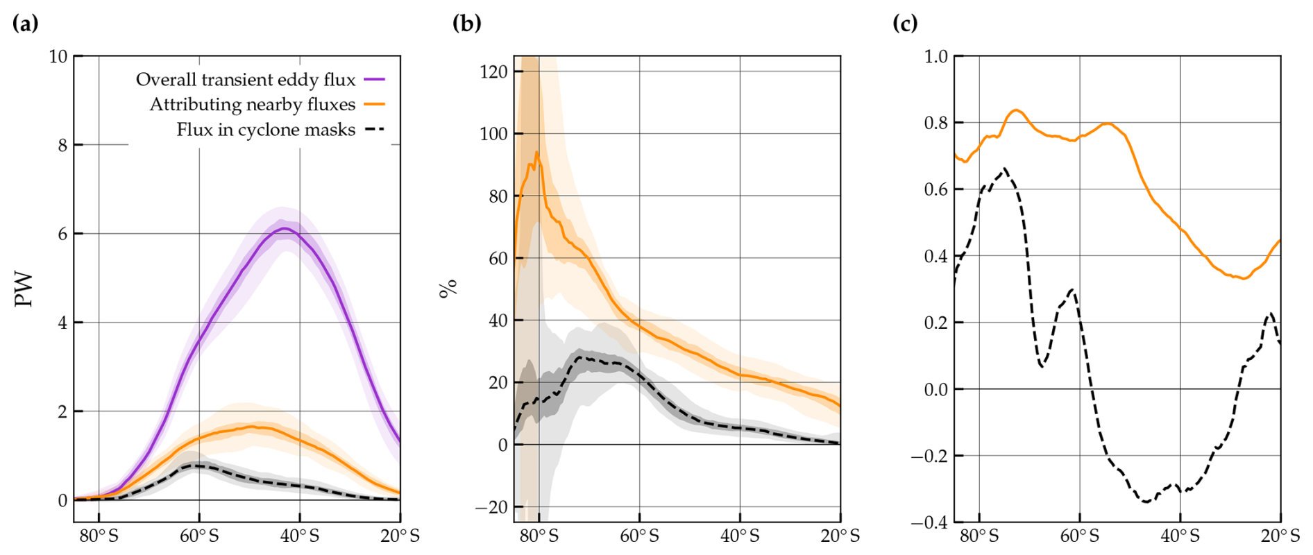
Figure 7 Seasonal transient MSE fluxes in SH winter: (a) the overall transient MSE fluxes, $\langle \left[{\stackrel{\mathrm{‾}}{v^{\prime }{m}^{\prime }}}_{\mathrm{MA}}\right]\rangle$, shown in purple are contrasted to the transient MSE fluxes within features that are attributed to cyclones, $\langle \left[{\stackrel{\mathrm{‾}}{v^{\prime }{m}^{\prime }}}_{\mathrm{MA}}^{\text{cycl}}\right]\rangle$ (orange) and the transient MSE fluxes within cyclone masks (black, dashed). Solid and dashed lines indicate medians, light shading the full range, and darker shading the inter-quartile range of the seasonal means. (b) The percentage of the overall transient MSE flux attributed to cyclones (orange) and within the cyclone masks (black). (c) Correlations between seasonally averaged overall transient MSE fluxes and the fraction attributed to cyclones using the overlap method (orange) and with the SLP-based cyclone masks (black dashed).

Confirming expectations from the composites, in the zonal integral the transient MSE flux located within the SLP-based cyclone masks is less than 1 PW (black dashed line in Fig. 7a) amounting to only ≈ 10 % of the transient MSE flux at 50° S (Fig. 5b). Accordingly, a low or even negative correlation is found between the seasonally averaged total and transient MSE fluxes within only the cyclone mask (black line in Fig. 7c). Based on the overlap method, the cyclone-attributed MSE fluxes peaks at around 50° S, and therefore much closer to the MSE flux maximum near 42° S, whereas the fluxes within the SLP-based cyclone masks peak much further poleward (62° S). This is consistent with the fact that transient MSE flux is most pronounced equatorward of the cyclone center along the trailing fronts as indicated in the composites. By bridging the latitudinal gap between the surface cyclone tracks and transient MSE fluxes (see also Fig. 1b), the overlap attribution method is a comprehensive solution to connecting the two storm track metrics. Qualitatively, the results are robust relative to the choice of the percentile and flux decomposition method (see Sect. S4, Fig. S5).

4.2 Relevance of cyclone life cycle characteristics for the zonally integrated MSE flux

Next, we address how life cycle characteristics influence the contribution of individual cyclones to the zonally integrated MSE flux. The contribution of a cyclone is defined as the attributed MSE flux along the track over the cyclone lifetime. We compare the accumulated MSE flux of the top 25 % of cyclones to the bottom 25 % for each life cycle characteristic.

At 50° S, the lifetime-accumulated transient MSE flux of the 25 % most strongly intensifying cyclones corresponds to ≈ 23 PW h (blue solid line in Fig. 8a). In turn, the 25 % of cyclones with the lowest intensification rates on average accumulate an MSE flux of only a few PW h, which peaks further poleward at around 65° S (red solid line in Fig. 8a). Thus, cyclones intensifying strongly accumulate 2.5–15 times the zonally integrated transient MSE flux of weakly intensifying cyclones (solid purple line in Fig. 8b).

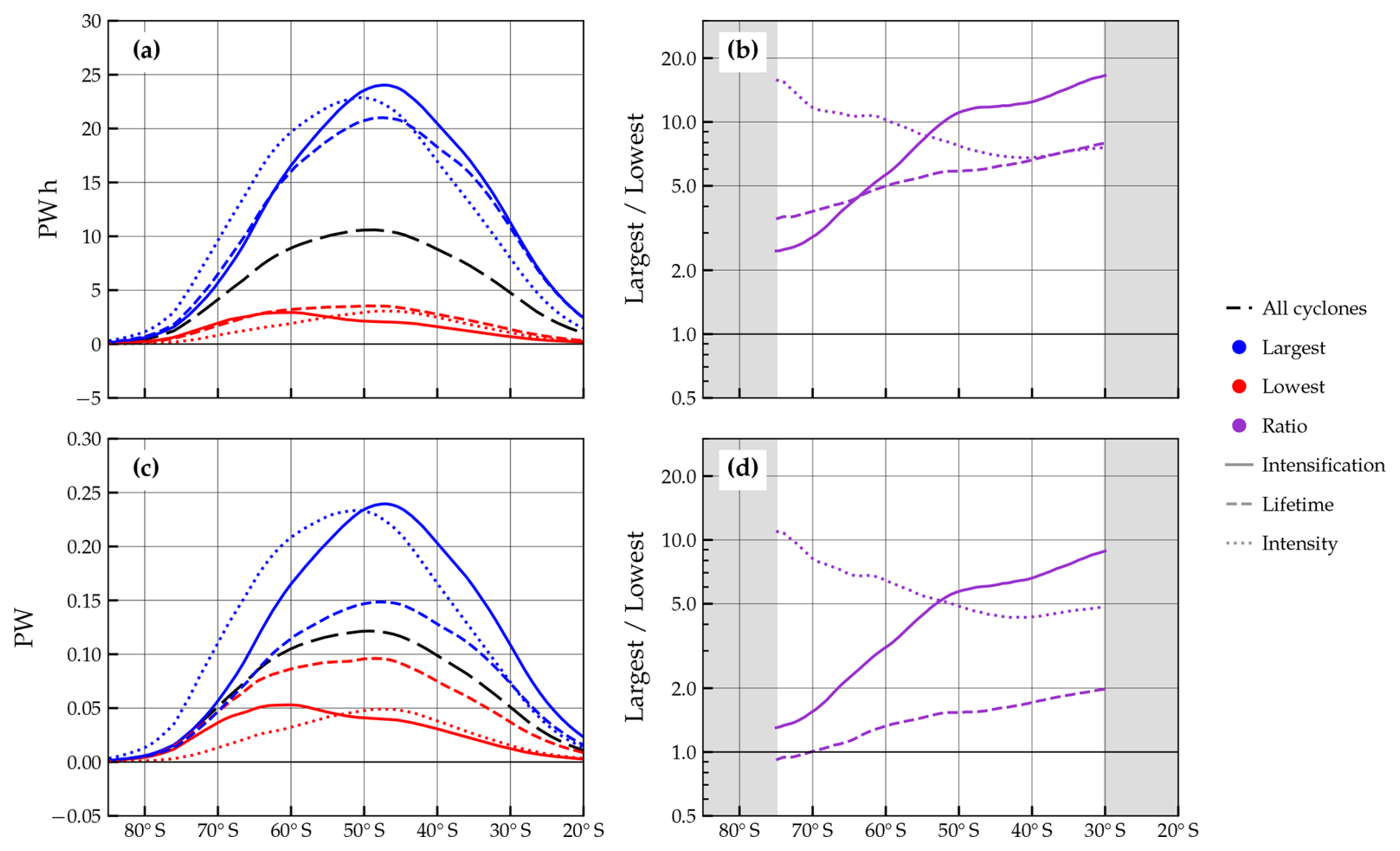
Figure 8 (a) Average zonally and vertically integrated transient MSE flux attributed to extratropical cyclones, $\langle \left[v^{\prime }{m^{\prime }}_{\mathrm{MA}}^{\mathrm{cycl}}\right]\rangle$, grouped by characteristic. Instantaneous vertically integrated fluxes are integrated temporally over the lifetime of each cyclone and integrated longitudinally at each latitude (unit PW h). For each characteristic, the flux of the top 25 % of cyclones is shown in blue and the bottom 25 % ones in red, respectively. Solid, dashed, and dotted lines indicate intensification rate, lifetime, and intensity, respectively. For example, the most intense cyclones are shown by the blue dotted line. (b) Dividing the flux of the top 25 % of cyclones by the flux of the bottom 25 % yields the ratio for each characteristic with the same line-styles as in panel (a). (c, d) As in panels (a) and (b), respectively, but for the average flux per time step in PW. In panels (a), (c), the average fluxes computed from all SH JJA cyclones (from which the other subsets are chosen) are shown with black long dash lines. The ratio in panels (b) and (d) is masked out at latitudes where the absolute fluxes are close to zero.

Similarly, the ratio between the fluxes attributed to the cyclones of longest vs. shortest lifetimes is generally well above 3 (dashed line in Fig. 8b). Cyclone intensity also emerges to be a clear differentiator for accumulated transport and exceeds the intensification rate poleward of 50° S. The fluxes of the most intense cyclones are also located further poleward compared to the weakest cyclones (dotted lines in Fig. 8a). In contrast to the intensification rate, the ratio corresponding to intensity thus increases towards the pole (Fig. 8b).

To rule out the possibility that the strongly intensifying and intense cyclones show large MSE fluxes simply because of long lifetimes, we also compare lifetime-averaged MSE fluxes. These are simply computed by normalizing the accumulated flux of each cyclone by its lifetime. On average, this flux amounts to 0.12 PW at 50° S (black dashed line in Fig. 8c). Note that during each winter season, around 340 unique cyclones are identified. These have an average lifetime of 3.4 d, such that 12.5 cyclones are present at an instant on average⁴. The estimated 1.5 PW that they contribute altogether matches the seasonal mean attributed flux shown in Fig. 7a.

It is found that strongly intensifying cyclones are associated with a lifetime-averaged flux of ≈ 0.23 PW which peaks between 45 and 50° S (solid lines in Fig. 8c). The least intensifying cyclones transport roughly 6 times less at this latitude (Fig. 8d). Conversely, the lifetime-averaged fluxes attributed to the most long- and short-lived cyclones are more comparable (dashed lines in Fig. 8c) and approach the average of all SH cyclones. The ratio of the attributed fluxes of these sets is systematically below 2 (Fig. 8d) which is much lower than for the corresponding lifetime-accumulated fluxes. The ratio between the most and least intense cyclones (dotted lines) is also reduced compared to the accumulated fluxes but still amounts to ≈ 5 around 50° S. As for the lifetime-accumulated MSE fluxes, the MSE fluxes of the most intense cyclones are larger than those of the most strongly intensifying cyclones poleward of ≈ 50° S. It can be concluded that although the cyclone lifetime can matter for the lifetime-accumulated MSE flux, the large fluxes attributed to the strongly intensifying (or intense) cyclones arise from large fluxes at individual time steps.

In summary, the cyclone intensification rate and intensity strongly imprint in the zonally integrated MSE flux attributed to individual cyclones. While the previous composite analyses highlighted the importance of the cyclone intensification rate, poleward of ≈ 50° S the attributed MSE fluxes of the most intense cyclones are larger. Generally, the conclusions do not qualitatively depend on the parameter choices of the applied decomposition method or flux attribution threshold (the latitude at which intensity dominates over intensification rate varies between 40 and 60° S, for instance, but intensity is always dominant on the poleward side, see Fig. S7). A logical next step is to assess whether these sets of cyclones also modulate the zonally integrated MSE flux on the seasonal scale.

5 The relationships between MSE fluxes and cyclone numbers on the seasonal scale

Finally, we investigate the relationship between extratropical cyclones and the zonally and vertically integrated transient MSE flux, $\langle \left[v^{\prime }{m^{\prime }}_{\mathrm{MA}}\right]\rangle$, on a seasonal scale. Given that large transient MSE fluxes can be attributed to strongly intensifying and intense cyclones, we test the hypothesis that the seasonal number of these storms relates to the seasonal mean zonally integrated transient MSE flux. To ultimately relate cyclone numbers to the zonally integrated heat budget, we also inspect the relationship between cyclone numbers and the total (i.e., not just the transient) MSE flux. The seasonally averaged transient MSE flux attributed to cyclones is denoted with $\langle \left[{\stackrel{\mathrm{‾}}{v^{\prime }{m}^{\prime }}}_{\mathrm{MA}}^{\mathrm{cycl}}\right]\rangle$ as above. In the following, the focus is on the latitude of 50° S which corresponds to the peak of the cyclone-attributed transient MSE fluxes (Fig. 7a) and where the intense and strongly intensifying cyclones both show comparable flux contributions (Fig. 8a, c). We classify cyclones as “strong”, “moderate”, and “weak” consistently with the previous result sections and select seasonal subsets from the corresponding climatological sets as detailed in Sect. 2.5.

5.1 Seasonal cyclone numbers and seasonally averaged transient MSE flux

At 50° S, cyclones that intensify strongly account for around 47 % of the cyclone-related transient MSE flux in a season, i.e., $\langle \left[{\stackrel{\mathrm{‾}}{v^{\prime }{m}^{\prime }}}_{\mathrm{MA}}^{\mathrm{cycl}}\right]\rangle$ (yellow box in Fig. 9). This fraction is matched by the intense cyclones while the seasonal spread is slightly larger. For moderately intense cyclones and moderately intensifying cyclones (defined from the 25th to 75th percentile), the fractional contributions lies within the 40 %–50 % range (grey boxes in Fig. 9). Their contribution to the seasonal mean MSE flux is thus slightly weaker than the contribution by the strong and strongly intensifying cyclones, although they are (on average) twice as numerous. In turn, weak and weakly intensifying cyclones only account for only around 10 % of the attributed fluxes in a season.

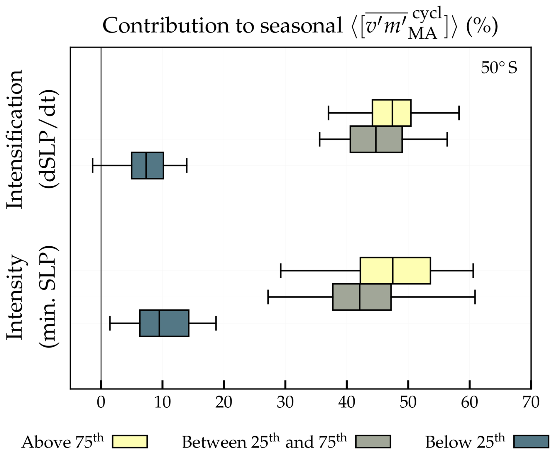
Figure 9 Contributions of cyclones within three different ranges of intensification rate (top) and intensity (bottom) to the seasonal transient MSE flux that is attributed to cyclones ($\langle \left[{\stackrel{\mathrm{‾}}{v^{\prime }{m}^{\prime }}}_{\mathrm{MA}}^{\mathrm{cycl}}\right]\rangle$). For each life cycle characteristic, cyclones are grouped seasonally by the 25th and 75th percentiles derived from the climatological sets of cyclones that have non-zero $\langle \left[{\stackrel{\mathrm{‾}}{v^{\prime }{m}^{\prime }}}_{\mathrm{MA}}^{\mathrm{cycl}}\right]\rangle$ at this latitude. The seasonal fluxes attributed to the cyclones that lie above the 75th percentile are represented in yellow, the ones between the 25th and 75th in grey, and the ones below the 25th in blue. Medians are shown with solid lines within the boxes that denote the interquartile range. Whiskers indicate 1.5 times the interquartile range while values outside of this range are not shown. MSE fluxes and cyclone numbers correspond to 50° S.

The above results may suggest an almost linear relationship between intensification rate and transient MSE flux: in the case of a linear relationship, one would expect the cyclones above the 75th percentile to contribute approximately 44 % to the budget.⁵ The flux indeed increases with cyclone intensification rate and intensity. However, for cyclones intensifying very rapidly the relationship is found to be non-linear, while it is rather exponential for intensity (not shown). Further, the intensities are not equally distributed but follow a (skewed) normal distribution for both characteristics. In sum, the identified fractions mean that the strongest cyclones contribute disproportionally compared to their frequency, which agrees with the conclusions in Messori and Czaja (2015). Yet, despite the large contribution to the zonal budget by the strong cyclones, still roughly half of the seasonal $\langle \left[{\stackrel{\mathrm{‾}}{v^{\prime }{m}^{\prime }}}_{\mathrm{MA}}^{\mathrm{cycl}}\right]\rangle$ results from moderate cyclones. This suggests that the number of strong cyclones has only a weak control on the zonally-integrated seasonal mean budget of transient MSE flux that can be associated with extratropical cyclones.

Indeed, in the MA framework the seasonal zonally and vertically integrated transient MSE flux attributed to cyclones, $\langle \left[{\stackrel{\mathrm{‾}}{v^{\prime }{m}^{\prime }}}_{\mathrm{MA}}^{\mathrm{cycl}}\right]\rangle$, is neither highly correlated with the number of strongly intensifying nor the number of intense cyclones (Fig. 10b and c). Conversely, $\langle \left[{\stackrel{\mathrm{‾}}{v^{\prime }{m}^{\prime }}}_{\mathrm{MA}}^{\mathrm{cycl}}\right]\rangle$ is correlated with the total cyclone number at this latitude (Fig. 10a).

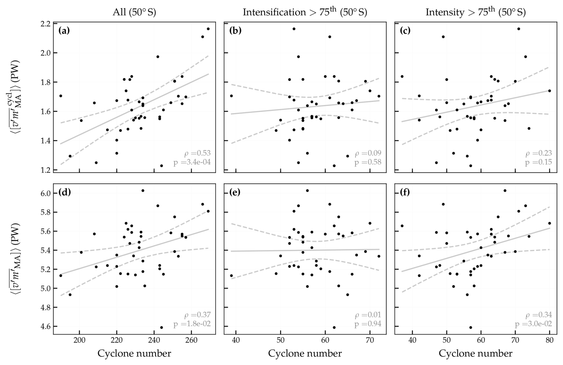
Figure 10 Relationship between seasonally averaged transient MSE flux and cyclone numbers for SH JJA at 50° S. (a) The cyclone-attributed transient MSE flux $\langle \left[{\stackrel{\mathrm{‾}}{v^{\prime }{m}^{\prime }}}_{\mathrm{MA}}^{\mathrm{cycl}}\right]\rangle$ (units of PW) and the number of all cyclones with $\langle \left[{\stackrel{\mathrm{‾}}{v^{\prime }{m}^{\prime }}}_{\mathrm{MA}}^{\mathrm{cycl}}\right]\rangle \ne \mathrm{0}$ at that latitude. (b, c) as panel (a) but for the number of strongly intensifying cyclones and intense cyclones, respectively. (d)–(f) as panels (a)–(c) but for the overall transient flux $\langle \left[{\stackrel{\mathrm{‾}}{v^{\prime }{m}^{\prime }}}_{\mathrm{MA}}\right]\rangle$. The grey solid line represents a best estimate of a linear fit and dashed grey lines the corresponding confidence band. Correlation (ρ) and p value of the slope of the linear fit (p) are indicated in each panel.

It is possible that an influence of the number of strongly intensifying or intense cyclones on the seasonal mean transport is obscured by shortcomings of the attribution method. Thus, we additionally inspect the relationships between the cyclone numbers and the overall transient MSE flux ($\langle \left[{\stackrel{\mathrm{‾}}{v^{\prime }{m}^{\prime }}}_{\mathrm{MA}}\right]\rangle$) to examine whether cyclones might influence the seasonal mean MSE flux also via the non-attributed flux. When correlating the total number of cyclones at 50° S with the overall transient MSE flux, $\langle \left[{\stackrel{\mathrm{‾}}{v^{\prime }{m}^{\prime }}}_{\mathrm{MA}}\right]\rangle$, the correlation remains positive albeit weaker than the previous result based on the cyclone-attributed flux (cf. Fig. 10a and d). Similarly to the cyclone-attributed flux $\langle \left[{\stackrel{\mathrm{‾}}{v^{\prime }{m}^{\prime }}}_{\mathrm{MA}}^{\mathrm{cycl}}\right]\rangle$, the overall flux $\langle \left[{\stackrel{\mathrm{‾}}{v^{\prime }{m}^{\prime }}}_{\mathrm{MA}}\right]\rangle$ is not correlated with the number of most rapidly intensifying cyclones (Fig. 10e). The correlation is higher, in turn, for the number of the most intense cyclones (cf. Fig. 10c and f). Omitting the flux attribution with the MA framework suggests that a comparable fraction of the seasonal variance in the overall transient MSE flux is explained by both the number of all cyclones and the number of intense cyclones (Fig. 10d).⁶ To this end, it is not clear why the correlation with the number of intense cyclones should be higher than with the number of strongly intensifying cyclones even though the fraction of the seasonal mean flux is, on average, practically equal.

As indicated, these relationships are specific to the MA framework. It is important to point out that the correlations vary substantially with flux attribution percentile and flux decomposition method (see Fig. S8, especially panels b, f, h). These analyses are also carried out defining transient MSE fluxes from high-pass filtered fields (HP) and, separately, from zonal anomalies (ZA). For the flux attributed using percentile rank p = 0.9, the correlation between the cyclone-attributed fluxes and the number of all cyclones, $\mathit{\rho }\left(\langle \left[{\stackrel{\mathrm{‾}}{v^{\prime }{m}^{\prime }}}_{\text{HP}}^{\mathrm{cycl}}\right]\rangle ,n_{\text{all}}\right)$, equals 0.35, while $\mathit{\rho }\left(\langle \left[{\stackrel{\mathrm{‾}}{v^{*}{m}^{*}}}_{\text{ZA}}^{\mathrm{cycl}}\right]\rangle ,n_{\text{all}}\right)=\mathrm{0.71}$ (Fig. S8b). Similarly, for the same percentile $\mathit{\rho }\left(\langle \left[{\stackrel{\mathrm{‾}}{v^{\prime }{m}^{\prime }}}_{\text{HP}}\right]\rangle ,n_{\text{all}}\right)=\mathrm{0.28}$ is considerably lower than $\mathit{\rho }\left(\langle \left[{\stackrel{\mathrm{‾}}{v^{*}{m}^{*}}}_{\text{ZA}}\right]\rangle ,n_{\text{all}}\right)=\mathrm{0.60}$. The correlation between overall transient MSE fluxes and the number of intense cyclones, $\mathit{\rho }\left(\langle \left[{\stackrel{\mathrm{‾}}{v^{\prime }{m}^{\prime }}}_{\text{HP}}\right]\rangle ,n_{\text{intense}}\right)$, is at least 0.48, whereas $\mathit{\rho }\left(\langle \left[{\stackrel{\mathrm{‾}}{v^{*}{m}^{*}}}_{\text{ZA}}\right]\rangle ,n_{\text{intense}}\right)\le \mathrm{0.37}$ across all considered percentiles (Fig. S8h). It is not surprising to find low correlations with the number of intense (or strongly intensifying) cyclones for an individual flux decomposition method given the large fraction of flux attributed to the cyclone sets of moderate intensity (or intensification, Fig. 9). The method dependency, however, was not expected, and the physical mechanisms thought to be responsible for this behaviour are discussed in Sect. 6.2.

5.2 Cyclone numbers and total MSE flux

On the six-hourly timescale, the transient and overturning circulations are temporally anti-correlated in the midlatitudes (Cox et al., 2024b). One could argue that the splitting into eddy and mean overturning circulation is therefore not strictly related to circulation features (e.g., cyclones, anticyclones, troughs, and ridges), which naturally contain signals from eddy and mean components because the mean was computed including the eddies in the first place. Thus, we also investigate the total MSE flux, $\langle \left[\stackrel{\mathrm{‾}}{vm}\right]\rangle$ (the left-hand side of Eq. 2), instead of the transient MSE flux. We continue to count cyclones as above using the latitudinal extent of their attributed transient MSE fluxes.

For the total MSE flux at 50° S, the correlation with the total cyclone number of cyclones passing through this latitude is 0.67. Of the latitude bands tested, 50° S is the latitude where this correlation is largest (Fig. S9j). The decrease towards the pole is not fully understood but potentially is connected to the increasing importance of planetary-scale relative to synoptic-scale related MSE fluxes that increases towards the pole (Stoll et al., 2023). Note that when simply taking the number of all cyclones in the entire SH instead of the number of cyclones only at 50° S the correlation reduces (Fig. S9i). This suggests that capturing the latitudinal extent of cyclones as shown in Fig. 2 is important.

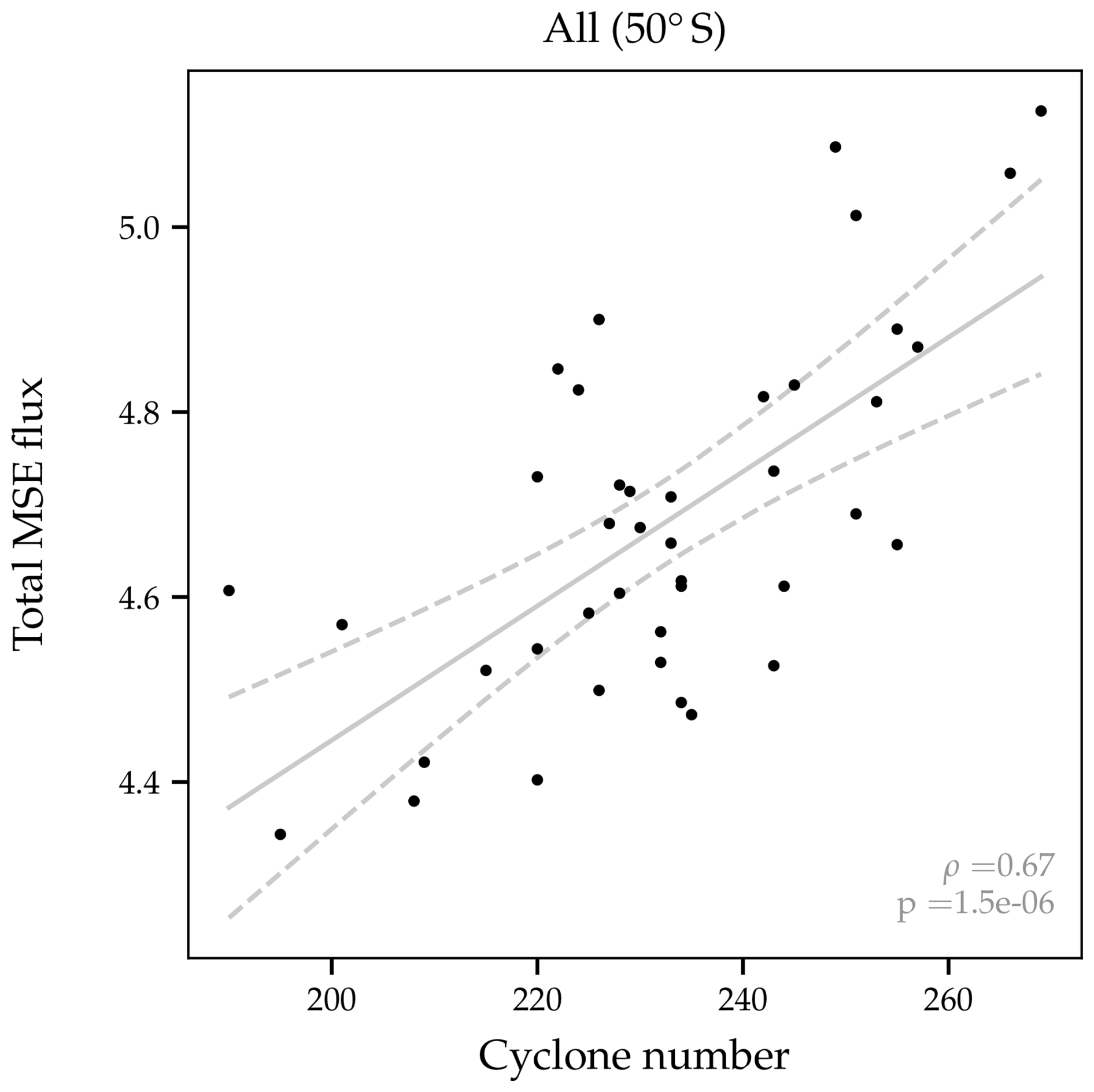
Figure 11 Relationship between seasonally averaged, zonally integrated total MSE flux, $\langle \left[\stackrel{\mathrm{‾}}{vm}\right]\rangle$, at 50° S (PW) and number of cyclones with a non-zero transient MSE flux attributed to them ($\langle \left[{\stackrel{\mathrm{‾}}{v^{\prime }{m}^{\prime }}}_{\mathrm{MA}}^{\mathrm{cycl}}\right]\rangle \ne \mathrm{0}$) at the same latitude. Grey solid and dashed lines as in Fig. 10. The correlation (ρ) and the p value of the slope of the linear fit (p) are indicated on the panel.

To sum up, no robust relationship between the seasonal number of intense or strongly intensifying cyclones and the seasonal transient MSE flux is identified. In contrast to the transient flux, the seasonal mean of the total zonally integrated MSE flux at 50° S exhibits a more robust correlation of 0.39–0.68 with the number of all cyclones passing that latitude. The correlation range results from the degrees of freedom in the counting method (cf. Fig. 2).

6 Summary and conclusions

6.1 Key findings

This study examines the relationship between zonally integrated heat transport and life cycle characteristics of extratropical cyclones during SH winter (JJA) using the ERA5 reanalysis. We have developed a novel method that combines the vertically integrated meridional transient eddy MSE flux with a feature-based cyclone tracking scheme. Specifically, the three central objectives of this study are: (i) to reveal the temporal evolution of the local meridional transient MSE fluxes during the cyclone life cycles; (ii) to quantify the contributions of cyclones to the zonally integrated transient MSE flux and assess how the contributions of individual cyclones vary depending on life cycle characteristics such as lifetime and intensification rate, and; (iii) to explore the relationship between cyclone numbers and MSE flux on the seasonal scale. In the following, the key findings are summarized.

• Locally, the meridional transient MSE fluxes peaks during the intensification phase and declines before the cyclone reaches its mature stage (Fig. 3), which is in agreement with the theory of baroclinic intensification (as is the vertical structure of the fluxes, cf. Gill, 1982). Cyclone-centered composites reveal large poleward MSE fluxes located in the warm sector confined between the warm and cold fronts and a smaller peak in the cold sector (Fig. 4). Furthermore, there is a clear positive relationship between the strength of the transient MSE flux and the intensification rate and maximum intensity of cyclones (Fig. 5). Crucially, a non-negligible fraction of warm-sector and cold-sector fluxes are located outside of the cyclone masks defined by closed SLP contours. Typically, warm-sector fluxes extend further equatorward and are spatially bound by the frontal zones. The poleward latent heat flux is, as expected, confined to the warm sector which leads to an increasing contrast between warm-sector and cold-sector MSE fluxes towards the equator (Fig. 6).

• In the zonal integral, the novel attribution method based on feature overlap attributes 30 % of the transient MSE flux to cyclones. This method places the latitudinal maximum in cyclone attributed MSE flux closer to the overall transient MSE flux relative to only counting the MSE flux within cyclone masks (Fig. 7). This supports the notion that large MSE fluxes associated with warm conveyor belts, which are located typically along the boundaries and outside of the cyclone masks, are important contributors to zonally integrated MSE transport as proposed in Messori and Czaja (2015). The most intense and most strongly intensifying cyclones have the largest fluxes attributed to them with intensity dominating poleward and intensification rate equatorward of 50° S, respectively (Fig. 8). As expected, the accumulated fluxes also increase with cyclone lifetime but cyclone lifetime is a much weaker indicator for the attributed flux than intensity or intensification rate, especially when it comes to the instantaneous zonally integrated fluxes. Previous research has found that the poleward propagation speed (and not necessarily intensity or intensification rate) is the characteristic for which the poleward moisture fluxes within a fixed radius around the center are the largest (Sinclair and Dacre, 2019). For MSE fluxes in this study, the cyclones with fastest poleward propagation speed show comparable lifetime-averaged fluxes to those of the most intense cyclones at some latitudes but not consistently larger ones (not shown).

• The identified link between cyclone intensity and attributed transient MSE fluxes also applies to the seasonal scale. Storms that have an intensity larger than the 75th climatological percentile collectively contribute to around 45 % of the seasonally integrated cyclone-attributed MSE flux (Fig. 9). The intense cyclones thereby transport roughly as much transient MSE flux as the moderately intense cyclones despite the latter being, on average, twice as numerous. However, the fraction of the MSE flux associated with the intense cyclones are not disproportionate enough so that their number alone does not shape the seasonal mean transient flux (Fig. 10). This behavior also holds true for cyclone intensification and is further discussed below. For the total MSE flux at 50° S, the correlation with the number of all cyclones at that latitude lies between 0.39 and 0.68 (Figs. 11 and S8j). However, the correlation is reduced at other latitudes (Fig. S9j) such that further research is needed to better understand whether changes in cyclone numbers can be related to atmospheric heat transport changes constrained by the Earth's energy imbalance.

The determined contributions of extratropical cyclones to the total MSE flux are summarized in Fig. 12: cyclones contribute to the high-frequency (or “transient”) eddy MSE flux which, depending on the flux decomposition, is accompanied by low-frequency (or “stationary”) background fluxes and the mean overturning circulation. The high-frequency eddy MSE fluxes attributed to cyclones can be linked to different subsets of cyclones based on their intensity or intensification rate. Other high-frequency eddy MSE fluxes not attributed to cyclones may occur far from the cyclone center (possibly along fronts), be linked to high pressure systems, or be unrelated to weather features with closed contours such as meandering zonal flows.

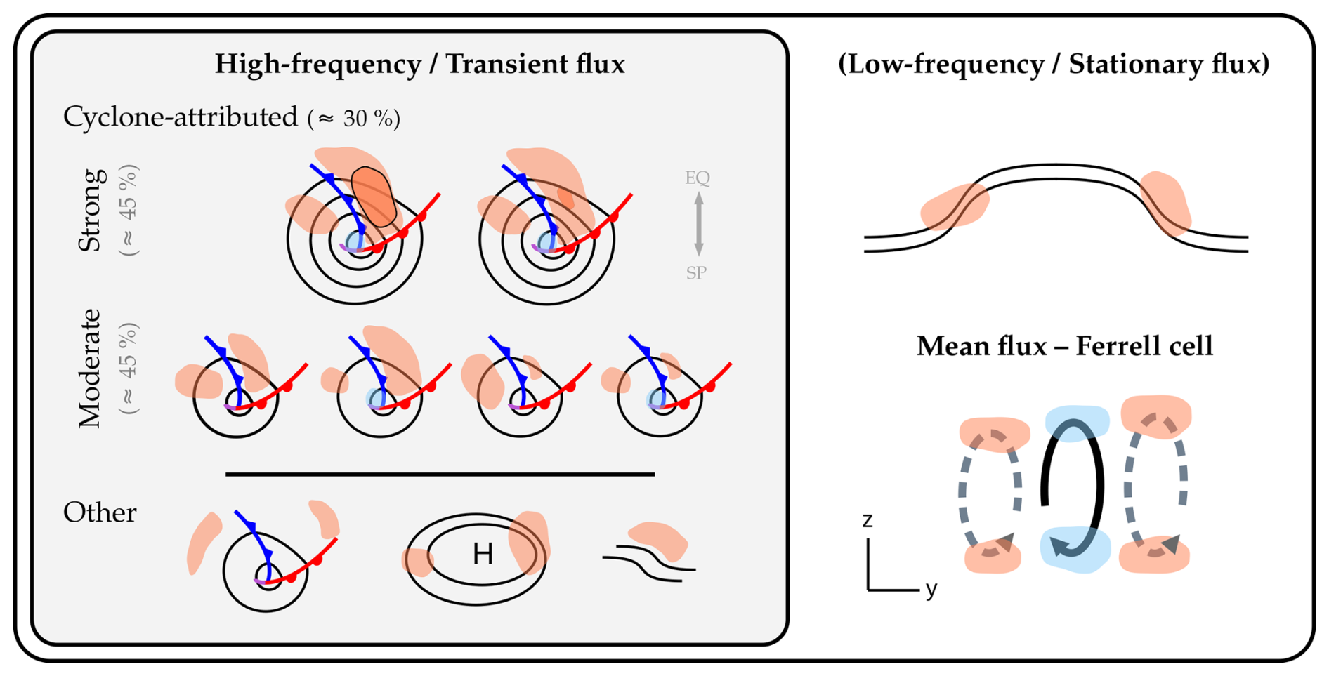
Figure 12 Schematic of the decomposition of total poleward atmospheric heat transport, which is described by the flux of MSE, into different flux components and contributions by extratropical cyclones: when adopting an eddy-mean decomposition, the total MSE flux is the sum of a high-frequency, transient eddy flux component, potentially a separate low-frequency or stationary eddy component, and the flux related to the mean overturning circulation. Orange and blue shading denotes poleward and equatorward meridional MSE fluxes, respectively. The high-frequency, transient eddy fluxes are further split into cyclone-attributed (≈ 30 % of the high-frequency eddy fluxes) and other fluxes. Surface cyclones in the left box are illustrated by SLP contours that are accompanied by warm fronts (red lines), cold fronts (blue), and occlusions (purple). “Strong” and “moderate” refer to the intensity or intensification rate of cyclones with “weak” cyclones omitted. Grey percentage indications refer to the approximate contribution of those cyclones to the cyclone-attributed eddy MSE flux (and not the overall high-frequency eddy flux). Low-frequency or stationary flow is sketched by wave-like black lines in the top right. In the bottom right, the zonal mean flux is drawn in a latitudinal and vertical y–z cross-section with the overturning circulation illustrated with solid black (Ferrell cell) and dashed grey (polar and Hadley cells) arrows.

6.2 Considerations on the choice of the eddy-mean decompositions

In the above summary, the conclusions are overall independent of the choice of eddy-mean decomposition method. A consequential method dependence in our study was only found for the correlation between the seasonal cyclone number and the transient MSE flux (Sects. 5 and S5). This points to a non-negligible influence of planetary, low-frequency waves to the local transient MSE flux attributed to individual systems as discussed below (Messori and Czaja, 2014; Stoll et al., 2023). Because some fraction of this background flux is attributed to an individual extratropical cyclone, the effect of its life cycle characteristics on the zonally integrated flux is partly masked. For large enough sample sizes, this method-dependency averages out (N > 700 as in Sects. 3 and 4), but the effect influences the result when considering a seasonal set of intense cyclones (N ≈ 60, Sect. 5).

When high-pass filtering, a wave-like signal with a frequency ∼ (11 d)⁻¹ is filtered out whereas in the zonal anomaly framework the corresponding flux is partly attributed to cyclones. It is found that the number of intense cyclones is more highly correlated with the high-pass filtered transient flux than the transient flux computed from zonal anomalies (regardless of whether only the cyclone-attributed or overall transient flux is considered, Fig. S8d, h). We argue that the lower correlation for the zonal anomaly method arises because part of the background flux is attributed to each cyclone – independently of cyclone intensification rate or intensity. In line with this argument, the addition of this background signal leads to a higher correlation between the seasonal fluxes and the overall cyclone number for the zonal anomaly method while the correlation for the high-pass filtering method tends to reduce (Fig. S8b, f). The monthly anomaly framework is a special case with the amount of background flows attributed to cyclones lying somewhere between the other two methods. As a result, the correlations generally fall within the two other methods (Fig. S8).

Our results may suggest that high-pass filtering is the most suitable decomposition method to investigate how extratropical cyclones contribute to the total MSE flux and to quantify their importance in the Earth's heat budget. Compared to the other methods, the choice of the cut-off frequency (or likewise the spatial wavenumber) can be motivated dynamically (e.g., Eady, 1949). However, some spectral power of a warm conveyor belt, for instance, is contained in the flow that is filtered out. As the spectrum of total MSE flux is predominantly continuous (see for instance the Supplement of Stoll et al., 2023), choosing a scale separation in time or space is a balance between how much low wavenumber flux is attributed to a background component and how much of it imprints in the transient component, eventually near individual cyclones. While high-pass filtering arguably isolates the synoptic signal best, it is also the method with the smallest fraction of total MSE flux explained by cyclone-attributed transient MSE flux (Fig. S5). If the goal is to describe and compare all MSE flux contributions in the fully closed atmospheric heat budget (Eq. 1), using a frequency filtering approach usually requires computing and investigating more interaction terms (e.g., Franzke and Harnik, 2023) than a Reynolds decomposition (Eq. 2). Thus, the choice of the eddy-mean decomposition method depends on the research question.

6.3 Avenues for methodological refinements and future research

One may argue that surface weather features are not responsible for the MSE flux throughout the entire vertical column. While we do not expect a strong influence of stratospheric fluxes on our results during SH winter (at 65° S, stratospheric fluxes account for only 11 % of the column-integrated fluxes explaining 10 % of its variance; Cardinale et al., 2021), a rigorous sensitivity analysis with respect to the vertical integration bound may offer further insight into the role of cyclones for the MSE flux at different levels. A possible hypothesis to test could be that excluding upper-level fluxes leads to a slightly higher correlation between the number of intense cyclones and high-pass filtered MSE fluxes on the seasonal scale.

Technically, the methods can readily be applied to the NH and other seasons as well. In the NH, the stationary (or low-frequency) signal is more pronounced due to the presence of land-sea contrasts and orography. This increases the sensitivity with respect to the flux decomposition method (for instance, in the composites; not shown). The contributions of low-frequency and planetary-scale waves to the zonally integrated MSE flux likely increase with height (Stoll et al., 2023) and stratospheric fluxes account for a larger fraction in the NH (Cardinale et al., 2021). Thus, a sensitivity analysis with respect to the vertical integration bound is even more relevant when examining the role of cyclones for MSE flux in the NH. Furthermore, when investigating zonally integrated fluxes one has to reflect on whether and how to disentangle the signals arising from the Atlantic and Pacific basins due to different changes in cyclone characteristics. The response of the cyclone number and storm track latitude to warming, for instance, is different in these two basins (e.g., Seiler and Zwiers, 2016; Chang, 2018).

As can be seen in the composites, the transient MSE fluxes do not peak exactly in center of cyclones but rather between cyclones and anticyclones. As all of the overlapping MSE flux is attributed to cyclones in our approach, we do not discuss the role of anticyclones for poleward MSE flux (Ruggieri et al., 2020). Instead of attributing fluxes to cyclones, future research may focus on the influence of warm and cold sectors (which are located between the cyclones and anticyclones) and the role of their numbers on the zonal heat budget. Warm and cold sector MSE fluxes could be identified using atmospheric river (Shields et al., 2018) or warm conveyor belt masks (using Lagrangian air parcel trajectories; Heitmann et al., 2024) and cold sector masks (Zolina and Gulev, 2003; Kolstad and Bracegirdle, 2008; Vannière et al., 2016), respectively. The fluxes within these features could still be attributed to cyclones in a second step which would yield a more sophisticated flux attribution that takes into account not only the temporal development of the cyclones but also of the flux events (e.g., Fearon et al., 2021; Lopez-Marti et al., 2025). To capture the MSE flux along the trailing fronts, one could attribute fluxes to cyclones directly via identified surface fronts (e.g., as in Papritz et al., 2014), although it is unclear how well these capture remaining fluxes throughout the sectors (Messori et al., 2017).

This study has not addressed trends in either MSE fluxes or cyclone numbers. The projected decrease of SH winter cyclones in a warmer climate, however, motivates further research on the relationship between extratropical cyclones and zonal mean energetics. This could involve relating trends in MSE fluxes (Rydsaa et al., 2021; Clark et al., 2022; Simmons, 2022; Franzke and Harnik, 2023; Cox et al., 2024a; Kang et al., 2024) to trends in cyclone numbers and life cycle characteristics (Karwat et al., 2022). Of course, as this work was motivated by the projected decrease in the extratropical cyclone number, a natural continuation of this work is to address it in the context of atmospheric heat transport. A follow-up study is planned of which the aim is to apply the newly introduced flux attribution method to idealized and fully-coupled climate simulations.