Sea-effect snowfall in the Baltic Sea area in 1998–2018 derived from convection-permitting climate model data

Sea-effect snowfall forms frequently over the Baltic Sea in northern Europe. In its bordering countries, large snow accumulations and poor visibility associated with these, often intense, convective snowbands have had considerable impacts on society. This study presents, for the first time, the occurrence of snowband days over the full Baltic Sea area on climatological time scales. The climatology is investigated using a 21 year long simulation made with the HARMONIE-Climate convection-permitting regional climate model applied at 3 km resolution. Snowband days are identified using a set of previously established criteria describing environmental conditions favorable for sea-effect snowfall, combined with an additional threshold on snowfall flux. Snowband days occur most frequently (up to a few days per year in a 3 km×3 km area) over specific regions of the Baltic Sea: near the eastern coast of Sweden, over the Gulf of Finland and the Northern Baltic Proper. Over the majority of the northern Baltic Sea, snowbands occur typically between November and February. Winds with an easterly component at the 900 hPa level favour the occurrence of snowbands along the eastern coast of Sweden and southern coast of Finland, whereas few cases in those regions occur with westerly winds. In addition, snowband days occur over the southern Baltic Sea, where the formation of snowbands is favoured by low-level winds having a northerly component and typically between December and March. This study provides useful context for operational forecasters and forms the basis for future research on how the occurrence of these events may change in a changing climate.

1 Introduction

Sea-effect snowfall (also commonly referred to as lake-effect snowfall) is convective precipitation that forms over ice-free water surfaces (e.g. seas and lakes) during the cold season. Under suitable wind conditions, the systems may drift from the sea to land. Intense sea-effect snowfall can cause significant damage to coastal infrastructure, with localized impacts such as structural damage from snow loading and reduced visibility leading to traffic disruptions. They may also result in more widespread consequences if critical infrastructure, such as the energy sector (e.g., nuclear power plants that are located at the coast), is affected.

The development of sea-effect snowfall systems is a complex process that is affected by the distribution of sea-ice, the temperature and wind distribution of the overlying airmass and the shape and size of the water basin. In order for sea-effect snowfall to form, the sea must be ice-free and there should be a large atmospheric lapse rate, i.e. decrease in temperature with height between the sea surface and the overlying airmass (Niziol, 1987). This situation typically occurs when a cold airmass moves over relatively warm sea, allowing for the destabilization of the air by strong surface fluxes of heat and moisture and the subsequent formation of convective updrafts. A generally applied rule of thumb is that the air temperature at the 850 hPa level should be at least 13 °C colder than the sea surface temperature (roughly equivalent to the dry adiabatic lapse rate) for sea-effect snowfall to develop (Markowski and Richardson, 2010; Holroyd, 1971). The development of updrafts may still be inhibited by the presence of inversion layers, or, further enhanced by mesoscale processes such as coastal convergence (Andersson and Nilsson, 1990) and orographic lifting (Solantie and Pirinen, 2006). Other factors contributing to the destabilization of air include the presence of moderate or strong low-level winds (increases surface fluxes) and a long fetch of air over the sea (more time for destabilization by surface fluxes). Over land, the convective updrafts typically quickly diminish due to the absence of the forcing surface fluxes, and therefore the resulting snowfall is usually limited to areas located within a few tens of kilometers inland from the coastline.

Sea-effect snowfall systems can take many shapes and sizes depending on the prevailing wind distribution, the shape of the sea and the orientation of the wind with respect to the coastline. The most intense systems typically manifest as long (up to a few hundred kilometers) and narrow (a few to tens of kilometers wide) snowbands, with cloud tops reaching approximately 5 km (Markowski and Richardson, 2010; Niziol et al., 1995). These types of snowbands typically form when the fetch is long and aligned with the low-level wind direction, and the wind shear, i.e. the change in wind speed and direction with height, is small. Preferably, the directional shear should not be larger than around 30° (Niziol, 1987; Niziol et al., 1995); in situations with stronger shear the systems usually take a more disorganized form or dissipate altogether (Niziol et al., 1995). As long as the large-scale atmospheric conditions and associated surface fluxes remain favorable (including an ice-free sea-surface), sea-effect snowfall may persist for several hours, occasionally up to several days, resulting in prolonged snowfall and potentially large snowfall amounts in coastal regions (e.g. Olsson et al., 2023, hereafter referred to as OLS2023).

Lake-effect snowfall is notorious especially in the Great Lakes region in North America (see e.g., Hjelmfelt and Braham, 1983), where it has been studied extensively. Considerable snowfall amounts caused by the sea-effect have been documented in the Baltic Sea region (Rutgersson et al., 2022), such as in Finland (Olsson et al., 2017, 2018; Juga, 2010; Juga et al., 2014; Niemelä, 2012; Mazon et al., 2015, and Olsson et al., 2020, hereafter referred to as OLS2020), Sweden (Jeworrek et al., 2017, hereafter referred to as JEW2017) and Poland (Bednorz et al., 2022). For example, in Finland, the current record for the highest measured daily snow depth increase (73 cm) was associated with a localized snowband making landfall over western Finland in January 2016 (Olsson et al., 2017). In eastern Sweden, multiple consecutive snowbands brought 130 cm of snowfall within a few days around the town of Gävle in December 1998, causing large societal impacts and economical losses (JEW2017, Westerblom, 2024). Furthermore, Japan is one of the snowiest regions globally due to frequent sea-effect snowfall (Steenburgh and Nakai, 2020). Sea-effect or lake-effect snowfall has also been observed, for example, along the Black Sea region in Turkey (Baltaci et al., 2021), the Caspian Sea (Ghafarian et al., 2018) and occasionally near the coast of the United Kingdom (Norris et al., 2013).

Identifying the long-term climatology of sea-effect snowfall in the Baltic Sea region is challenging due to the lack of continuous observational datasets with long temporal coverage (e.g. radar or satellite data). Furthermore, due to the small spatial and temporal scale of the systems, the resulting snowfall over land is often very localized and may thus be missed by weather observation stations near the coast. Consequently, existing climatologies for regions in the Baltic Sea area have primarily been based on indirect methods, or in other words, by finding the environments favourable for the occurrence of sea-effect snowfall from gridded climate model and reanalysis datasets (JEW2017, OLS2020, OLS2023). Accordingly, a snowband day has been defined as a day with environmental conditions favouring sea-effect snowfall.

The existing long-term climatologies of sea-effect snowbands in the Baltic Sea area have been limited to specific regions and typically constrained to prevailing wind directions that bring snowfall to the adjacent land (JEW2017, Bednorz et al., 2022, OLS2023). In Finland, OLS2023 used ERA5 reanalysis data (Hersbach et al., 2020) and snow depth observations to show that the whole Finnish coastline has experienced an annual average of 16 intense snowband days between 1973 and 2020, with most cases having occurred in November–December. Based on 11 years of data from a regional climate model, JEW2017 showed that over the eastern coast of Sweden, favorable conditions for snowbands with northerly to easterly winds occur on approximately 4 to 7 d yr⁻¹. In the study of JEW2017, the highest mean precipitation amounts during conditions favourable for sea-effect snowbands occur along the Swedish coastline of the Bothnian Bay, Bothnian Sea, and the western Gotland Basin, over Gotland, as well as over northern Poland (see regions in Fig. 1).

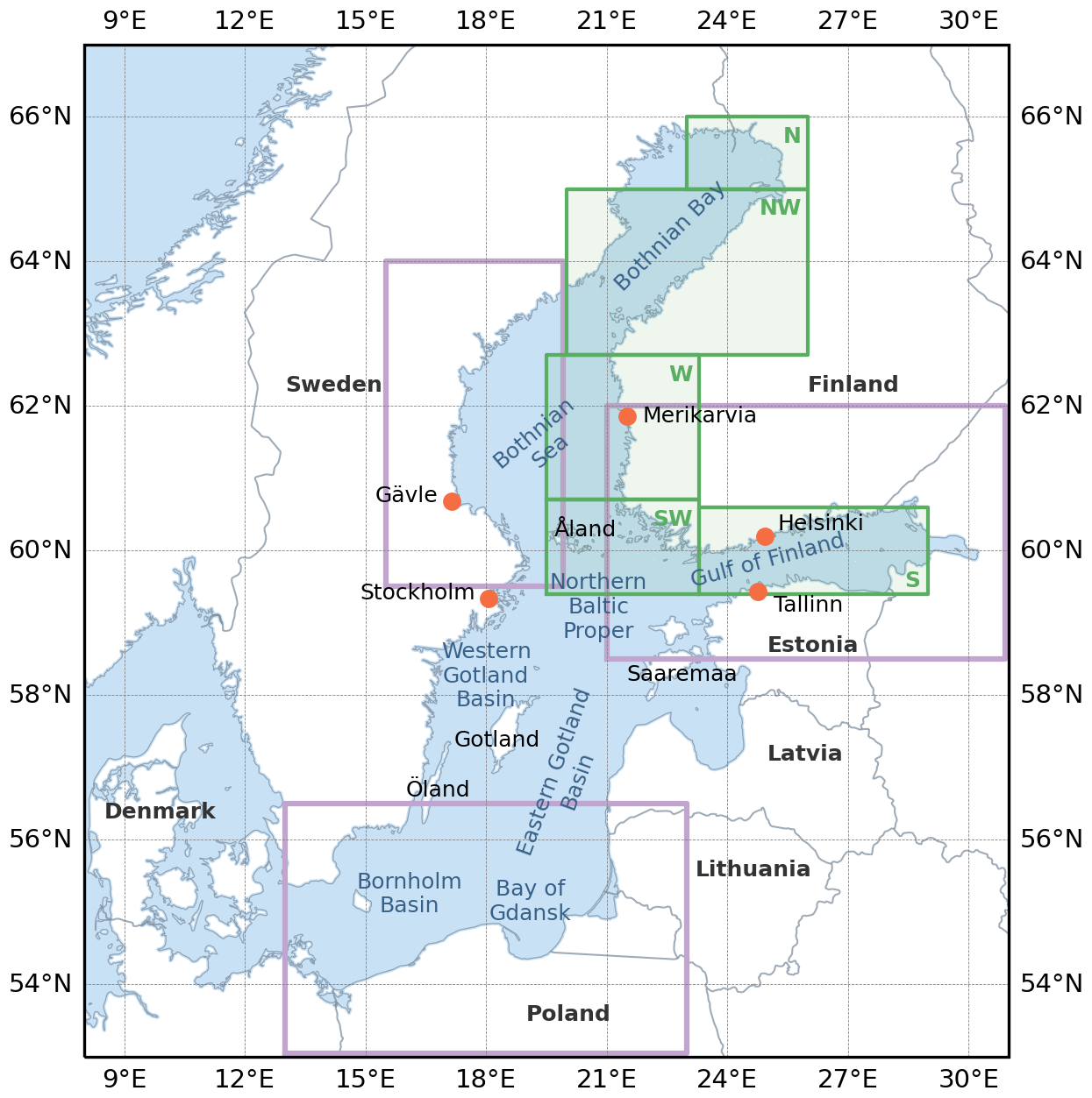
Figure 1 The study domain and the location of the subregions investigated in this study. Green boxes show the subregions defined by (Olsson et al., 2023, or OLS2023) and presented in Table 2 and Fig. 3. The shaded area corresponds to the area labeled as FI in the text and in Fig. 2. Purple boxes show the subregions presented in Figs. 9 and 10.

Previous studies on snowband statistics in Finland and Sweden are based on datasets created using weather and climate models having a spatial resolution much larger than individual convective updrafts. Recently, a 21 year climate simulation applied with 3 km horizontal grid spacing has been generated for the Nordic region with the HARMONIE-Climate (HCLIM) regional climate model (Lind et al., 2020). HCLIM uses non-hydrostatic dynamics and treats convective updrafts occurring on the grid scale or coarser explicitly, while using a parameterization scheme for sub-grid (shallow) convection. Such “convection-permitting” climate models with fine resolutions have been shown to lead to significant improvements in the representation of sub-daily convective precipitation (Lucas-Picher et al., 2021; Lind et al., 2020; Médus et al., 2022). Comparison to a wide range of observational datasets has shown that the convection-permitting HCLIM model, with reanalysis data as boundary conditions, simulates summertime daily precipitation distributions over Fennoscandia well and provides considerable added value to the statistics, amplitude and timing of hourly-scale extreme precipitation over Fennoscandia (Médus et al., 2022). Even though wintertime convection is typically less intense and shallower than in the summer, a convection-permitting climate model with high spatial resolution and non-hydrostatic dynamics is expected to provide added value for the simulation of the spatio-temporal evolution, structure, organization and intensity of convective precipitation systems also in the cold season compared to coarser models.

In this study, we utilize the convection-permitting HCLIM simulation, forced by ERA-Interim reanalysis data (Dee et al., 2011), to investigate the climatology of snowband days in the Baltic Sea area in 1998–2018. The goal is two-fold. First, we examine whether HCLIM can realistically simulate snowbands. To address this, we perform a qualitative comparison with the snowband day climatology that was defined by OLS2023 using ERA5 and snow depth observations and, in addition, examine the performance of HCLIM for a set of events from the recent past. Then, we apply the kilometer-scale HCLIM dataset across the entire Baltic Sea region to identify the general long-term spatial and temporal distribution of snowband days and the areas most at risk from sea-effect snowfall, as well as the synoptic environments associated with snowband days in selected regions. This enables us to complement existing snowband day climatologies for Finland and Sweden and, for the first time, to develop a 21 year climatology of sea-effect snowfall environments across the full Baltic Sea area.

This study is organized as follows. The HCLIM dataset and methodology used to detect snowbands is described in Sect. 2. Section 3 first presents results from the comparative analysis with a previously defined climatology (Sect. 3.1) and case studies of past snowband events over the Baltic Sea (Sect. 3.2). This is followed by an analysis of the long-term distribution of snowband days (Sect. 3.3), associated snowfall over the Baltic Sea (Sect. 3.4), and the corresponding snowfall and synoptic environment in selected regions (Sect. 3.5). The results are discussed in Sect. 4 and concluding remarks provided in Sect. 5.

2 Data and methods

2.1 HARMONIE-Climate (HCLIM) simulation

The HCLIM regional climate model is being developed and maintained in a consortium consisting of members from several national meteorological institutes in Europe (Lindstedt et al., 2015; Belušić et al., 2020) and is the climate version of the HIRLAM-ALADIN Research on Mesoscale Operational NWP in Euromed (HARMONIE) system (Bengtsson et al., 2017). Here, we use a pre-existing 21 year km-scale simulation made with HCLIM cycle 38 over Fennoscandia for the time period of 1998–2018, carried out as part of the Nordic Convection Permitting Climate Projections (NorCP) project and described in detail and evaluated in Lind et al. (2020), Olsson et al. (2021), and Médus et al. (2022).

The HCLIM convection-permitting simulation has been performed in a double nested approach; in the first step the global ERA-Interim reanalysis was downscaled using the HCLIM-ALADIN configuration at 12 km spatial resolution over a domain covering a large part of Europe and the eastern North Atlantic. The HCLIM-AROME configuration was then run with 3 km spatial resolution over an area covering Fennoscandia. The lateral boundary conditions from the HCLIM-ALADIN simulation were updated every 3 h. Both HCLIM model versions used 65 vertical levels and the SURFEX surface model (Masson et al., 2013).

It should be noted that while deep convection is treated explicitly in the convection-permitting configuration of HCLIM, shallow convection is still parameterized. Also, since the presence of sea ice is relevant for the formation (or not) of sea-effect snowfall, we briefly describe how sea-ice is treated in HCLIM cycle 38. Sea ice is parameterized using the Simple ICE (SICE) model (Batrak et al., 2018). In SICE, sea ice is represented as a slab of fixed thickness, with the prognostic temperatures across the ice layer computed by solving the vertical heat diffusion equation. Sea ice concentration and sea surface temperature are updated in conjunction with the lateral boundary conditions (here at 6 hourly intervals) in order to capture their long-term variability. Surface fluxes from a sea-tile grid cell are calculated as the weighted contributions from the ice-covered and open-water parameterization schemes. A more exhaustive description of the dynamics and physics parameterizations used in HCLIM cycle 38 can be found in Belušić et al. (2020) and references therein.

2.2 Sea-effect snowfall detection method

JEW2017 established a set of criteria that successfully identified snowband days from gridded climate model data along the east coast of Sweden. The criteria were based on extensive literature of the atmospheric conditions known to be key factors for the occurrence of snowbands (Holroyd, 1971; Niziol, 1987; Andersson and Nilsson, 1990; Niziol et al., 1995; Laird et al., 2003). Building on the work of JEW2017, previous literature of sea-effect snowfall and the analysis of four case studies of intense snowbands over the northern Baltic Sea using a convection-permitting numerical weather prediction model, OLS2020 and OLS2023 refined the snowband criteria to a set of conditions that statistically favour the occurrence of intense snowbands over the northern Baltic Sea.

We adopt the ingredients-based sea-effect snowfall detection method used previously by JEW2017, OLS2020 and OLS2023 to find snowband days over the Baltic Sea in September–May between 1998 and 2018. The detection method applies, at every 3 km×3 km grid box and 3 hourly timestep of HCLIM output data, a set of criteria for snowfall intensity and environmental conditions known to be favourable for the occurrence of sea-effect snowbands. If all criteria are fulfilled, that grid box and time step is counted as sea-effect snowfall. Days when all the criteria are fulfilled at at least one 3 hourly timestep (either in a grid box or within a subregion, see Sect. 3) are marked as snowband days. In order to accommodate the two-fold goal of this study, and to distinguish between intense snowbands and a wider range of sea-effect environments, we use three sets of criteria. The criteria are summarized in Table 1 and described in more detail below.

Olsson et al. (2023)Olsson et al. (2023)

Table 1 The criteria for meteorological parameters included in the sea-effect snowfall detection method. Note that Olsson et al. (2023, or OLS2023) included an eighth criterion for observed daily snow depth, but that criterion is not used in this study (see Sect. 2.2). Snowfall is given in liquid water equivalent.

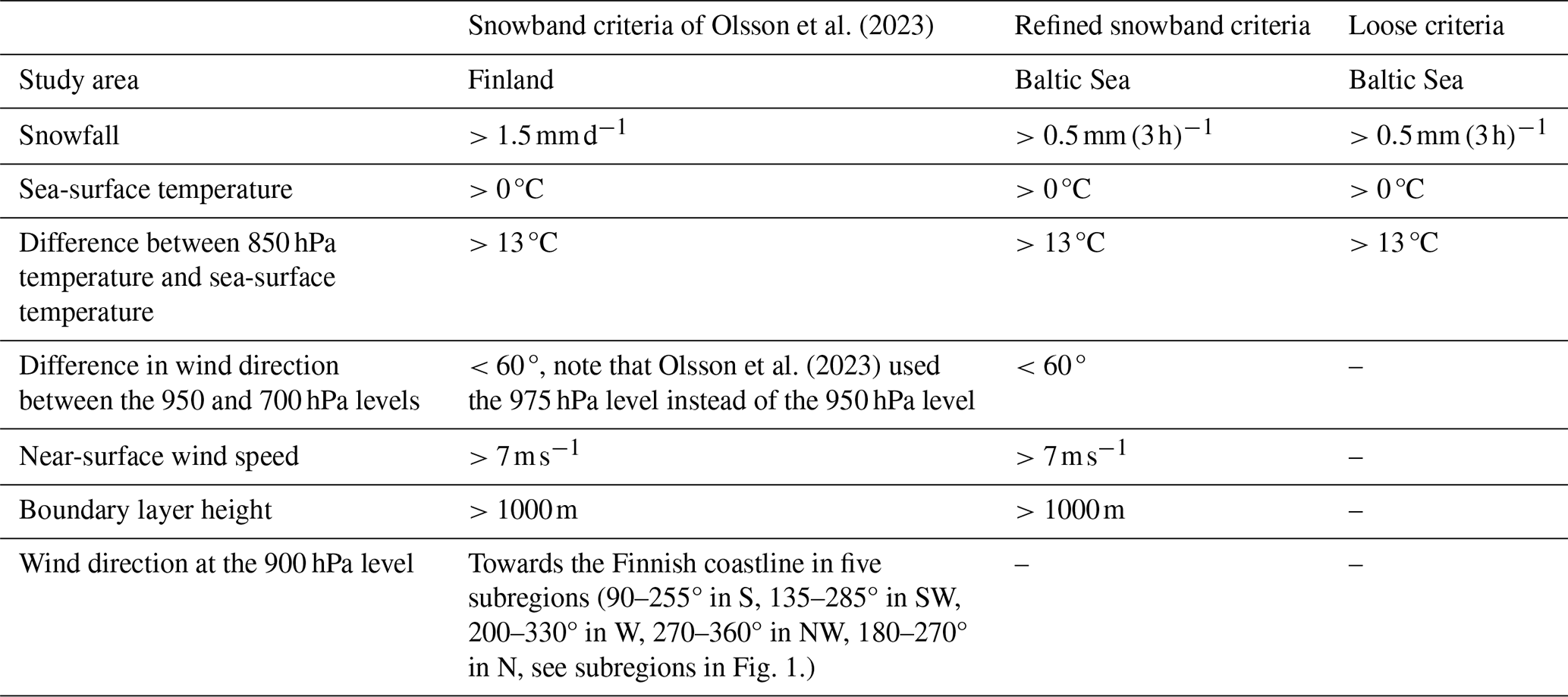
First, we use a similar set of criteria as OLS2023 to conduct a comparative analysis between HCLIM and the pre-existing climatology of snowband days along the Finnish coastline (Table 1, Sect. 3.1). OLS2023 divided the Finnish coastline into subregions depending on the orientation of the coast (N, NW, W, SW, S, and FI, see subregions in Fig. 1). In each grid box at every time step, criteria for sea-surface temperature, low-level temperature difference, directional wind shear, near-surface wind speed, boundary layer height, low-level wind direction and daily snowfall were checked. Sea-surface temperature should be greater than 0 °C and the vertical temperature difference between the sea surface and the 850 hPa level higher than 13 °C to increase the likelihood for an unstable airmass over an open water body. Near-surface wind speed is required to be stronger than 10 m s⁻¹ and directional shear weaker than 60° (defined here as the difference in wind direction between the 950 and 700 hPa levels) as moderate or strong low-level wind speed and weak directional shear is often associated with intense convective snowbands. Boundary layer height is required to be greater than 1 km and is used here as a proxy for conditions associated with strong surface fluxes and vigorous convection. To focus on cases where the convection results in snowfall flux at the surface, a threshold for snowfall was introduced, and OLS2020 and OLS2023 decided to use a daily threshold of 1.5 mm d⁻¹. Lastly, low-level wind direction (here defined at the 900 hPa level) was required to be towards the Finnish coastline in each subregion to focus solely on cases that drift towards the Finnish land areas. The snowband criteria of OLS2023 are similar to those from OLS2020. OLS2023 additionally required that observed daily snow depth must have increased at least 2 cm somewhere over land in the subregion. We replicate the criteria of OLS2023, but without the requirement for snow depth. Despite this difference, for the sake of clarity, we refer to this set of criteria as “the snowband criteria of OLS2023”.

Second, to investigate the climatology of snowband days over the whole Baltic Sea area with HCLIM (Sect. 3.3), we slightly refine the criteria of OLS2023. Instead of daily snowfall, we use a threshold for 3 hourly snowfall (calculated from the 3 h time period after the other criteria are fulfilled) and omit the criterion for the 900 hPa level wind direction. This ensures that the snow falls roughly at the same time as the environmental conditions are favourable for the occurrence of snowbands, increasing the likelihood that the detected cases are indeed sea-effect snowfall and not large-scale stratiform snowfall occurring earlier or later on the same day. By excluding the requirement for low-level wind direction, the study area can be expanded to the whole Baltic Sea. Hereafter, we refer to this set of criteria as “the refined snowband criteria”. Even though these criteria do not include wind direction, in the regional analysis presented in Sect. 3.3–3.5 detected snowbands will also be sampled according to the prevailing low-level wind directions.

As in OLS2020 and OLS2023, we focus on snowbands that are associated with a notable snowfall intensity. Defining an appropriate threshold for snowfall amount to capture intense snowbands is difficult and the number of cases can be expected to be sensitive to the threshold. We select the threshold of 0.5 mm (3 h)⁻¹ (in liquid water equivalent) and conduct a sensitivity test to the threshold (see Sect. 3.3). This threshold is between the median and 98th percentile of 3 hourly snowfall calculated from snowy timesteps (defined as time steps with snowfall amount over 0.01 mm (3 h)⁻¹) when all the other refined criteria except for the snowfall criterion are fulfilled (Fig. A1). The median of 3 hourly snowfall during timesteps with environmental conditions favourable for snowbands is generally between 0.03 and 0.12 mm (3 h)⁻¹, and the 98th percentile is between 0.6 and 1.2 mm (3 h)⁻¹ (Fig. A1). We note that, in this study, only snowfall is considered, whereas other solid precipitation types such as graupel are not included in the analysis.

Lastly, the above mentioned criteria adopted from previous studies have been designed to detect banded sea-effect snowfall (OLS2020, OLS2023). Sea-effect snowfall systems can take many shapes and sizes. To take into account a wider range of sea-effect snowfall environments and to test the sensitivity to the number of criteria used to detect the cases, we also include a brief analysis with a looser set of criteria. The loose criteria consider only the most important forcing mechanisms, namely, the sea-surface temperature >0 °C and the large temperature gradient between the surface and the overlying airmass which together drive the occurrence of strong surface fluxes of heat and moisture to the atmosphere. In addition to the sea-surface temperature and vertical temperature difference criteria, the 3 hourly snowfall rate is also included in the loose criteria analysis.

3 Results

3.1 Comparative analysis of snowband day climatologies

The monthly mean numbers of snowband days, as detected from HCLIM data using the criteria of OLS2023, on one hand, and as obtained from OLS2023, on the other hand, are presented in Fig. 2 for Finland (FI, see subregions in Fig. 1). Here, a snowband day is defined as a day during which the seven criteria adopted from OLS2023 are fulfilled in at least one grid box at least once per day somewhere in the subregion. Note that here only cases with wind direction favourable to bring snowfall over the Finnish coastline are included (see Table 1). The monthly distribution of snowband days in FI in HCLIM resembles that seen by OLS2023 (Fig. 2). In both data sets, snowband days are most frequent in November–January, with a peak in December. The number of snowband days is slightly higher in HCLIM than in OLS2023 in all months except for March–May, when HCLIM shows a lower number. We note that only a qualitative comparison between the current study and OLS2023 is possible as differences may arise from the different periods of investigation (1998–2018 in HCLIM and 1997–2020 or 1973–2020 in OLS2023), different spatial resolutions of the datasets (3 km in HCLIM and about 31 km in OLS2023) and lack of the criterion for snow depth in HCLIM. The larger number of cases in HCLIM may be, at least partly, explained by the slightly less strict criteria used compared with OLS2023.

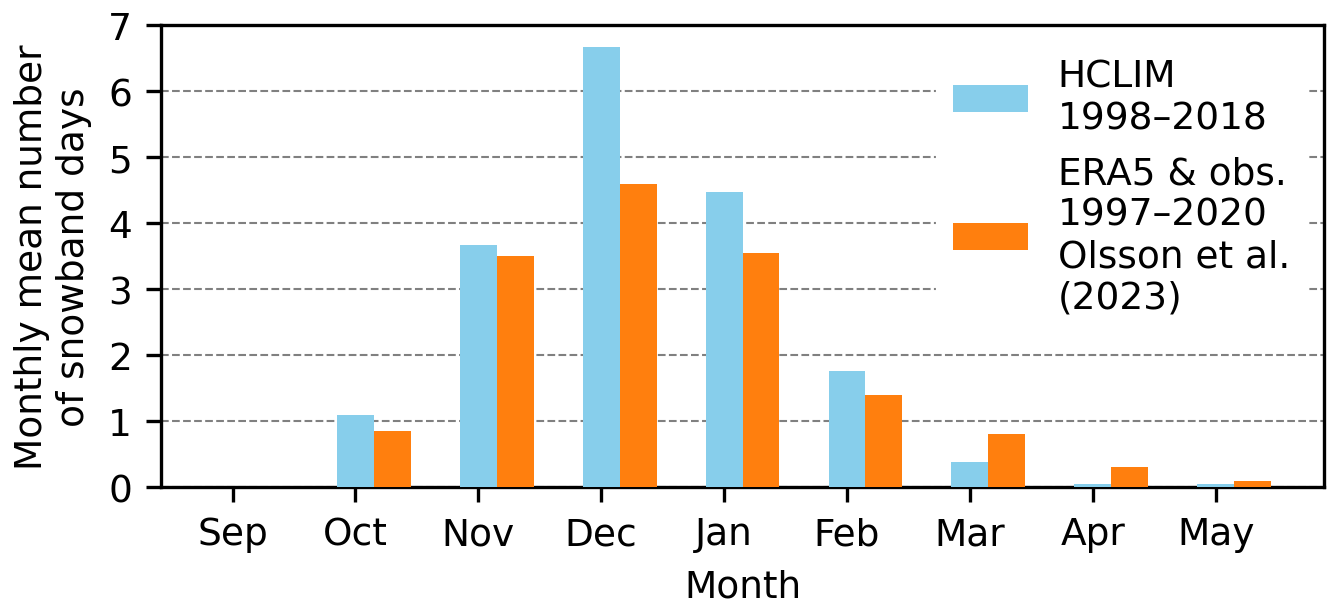
Figure 2 Monthly mean number of snowband days in Finland (FI, see subregion in Fig. 1) in HCLIM in 1998–2018 (blue) and that estimated from Fig. 2 of Olsson et al. (2023, or OLS2023, licensed under CC BY 4.0) using ERA5 reanalysis data and snow depth observations in 1997–2020 (orange). The snowband days are detected from HCLIM using the criteria of OLS2023 (see Table 1). Snowband day is defined here as a day during which all the criteria were fulfilled in at least one grid box at least once a day somewhere in FI.

The annual number of snowband days in FI varies considerably from year to year in both HCLIM and OLS2023 (Table 2). In HCLIM (1998–2018), the annual mean is 18 snowband days, with a range from 7 to 42. In OLS2023 (1973–2020), the mean is slightly lower at 16 snowband days, ranging from 6 to 40 annually.

Table 2 The average, minimum and maximum annual number of snowband days in Finland. The first column shows the subregions (see Fig. 1). The second, fourth and sixth column show the number of snowband days detected in HCLIM for the period 1998–2018 using the criteria of Olsson et al. (2023, or OLS2023, criteria given in Table 1) whereas the third, fifth and seventh columns present those adapted from Table 1 of OLS2023 (licensed under CC BY 4.0) for 1973–2020. Snowband days are defined here as days when all the criteria for snowbands are fulfilled in at least one grid box at least once per day somewhere in the subregion. Snowband days that were detected in multiple subregions were included only once in FI.

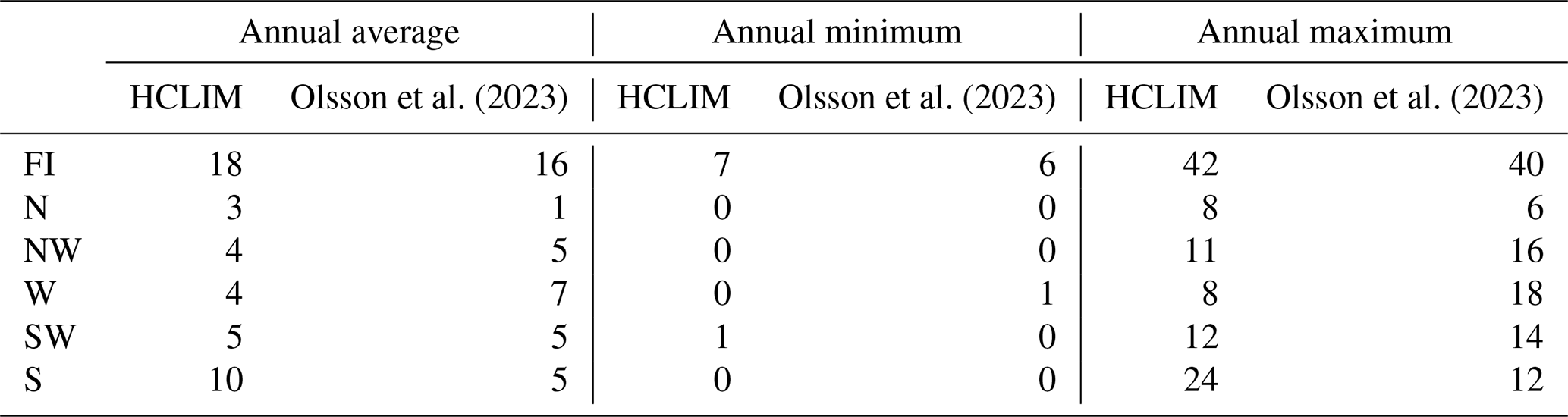
Although the annual and monthly mean numbers of snowband days in FI are quite similar in HCLIM and OLS2023, differences are seen within the smaller subregions (N, NW, W, SW and S). In HCLIM, the annual mean number of snowband days is largest in S, decreasing towards the north and is smallest in N (Table 2, note that the subregions vary in size and therefore quantitative comparison between the subregions is not straightforward). In OLS2023, the annual mean number of snowband days in 1973–2020 is more evenly distributed between the subregions and snowband days are most frequently detected in W (Table 2).

A closer inspection of the spatial distribution of snowband days (Fig. 3) defined using the criteria of OLS2023 shows that, in HCLIM, snowband days occur most frequently with easterly to southwesterly winds close to the southern coastline of Finland in S (with an annual average of one-to-two snowband days per 3 km×3 km area). In that region, OLS2023 shows a similar spatial distribution of snowband days (see Fig. 1 of OLS2023). However, in OLS2023, the most active region is located off the Finnish coastline in W, where the annual mean number of snowband days with south- to northwesterly winds was up to three. In HCLIM, no clear maximum is seen in W, and the annual mean number is much smaller (0–0.5 snowband days, Fig. 3). In SW and NW, HCLIM and OLS2023 show similar spatial patterns, though OLS2023 detects more frequent snowband days. In N, HCLIM shows a local maximum near the coast, while OLS2023 records fewer events.

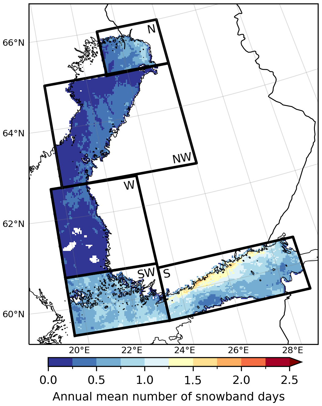
Figure 3 Annual mean number of snowband days in 1998–2018 in HCLIM detected by using the criteria of Olsson et al. (2023, or OLS2023, criteria given in Table 1). Snowband day in each grid box is defined here as a day during which all the criteria were fulfilled at least once.

3.2 Performance of HCLIM in case studies of past snowband events

One observed snowband event impacting Sweden and three from Finland were selected for a closer look to explore how well HCLIM, together with two sets of snowband criteria (the refined and the loose criteria, see criteria in Table 1), perform in simulating and capturing observed banded snowfall systems. The events are well covered in previous literature and have been verified as sea-effect snowbands. The findings from the case studies are described next and summarized in Sect. 3.2.5.

3.2.1 13 November 2007

The Swedish case occurred on 13 November 2007, when a long and narrow band of intense snowfall extended from the Gulf of Finland to the eastern coast of Sweden (observed radar reflectivity shown at 15:00 UTC in Fig. 4a). The radar reflectivity data for this case is obtained from the BALTEX Radar Data Centre (BRDC, Michelson et al., 2000), whereas the radar data for the three Finnish cases is provided by the Finnish Meteorological Institute. The snowband caused disruptions to traffic and slippery roads in regions south of Stockholm. In HCLIM, on 13 November 2007, a snowband extended all the way from southern Finland to south of Stockholm (shown at 15:00 UTC in Fig. 4b). The model snowband occurred in a synoptic environment with a surface low pressure situated over eastern Europe, leading to the advection of cold air from the north and northeast over the central Baltic Sea (Fig. A2a–b). The location and morphology of the snowband in HCLIM (Fig. 4b) closely resembles that of the observed system (Fig. 4a), and the same holds true also for the synoptic environment (Jungefeldt, 2020). The majority of the system was detected by both the refined and loose criteria (Fig. 4c–d).

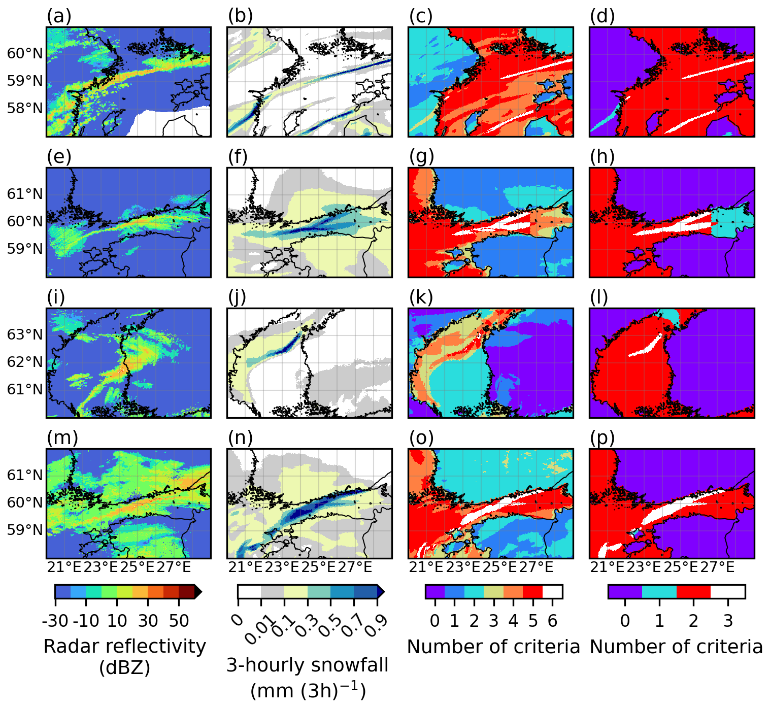
Figure 4 Observed radar reflectivity (dBz, first column), 3 hourly snowfall (mm (3 h)⁻¹) from HCLIM (second column) and the number of refined (third column) and loose (fourth column) criteria fulfilled at each grid box in HCLIM in the four case studies. Note that for a certain case study, the time and date in the first column may differ from that of the other columns. Namely, data is shown on 13 November 2007 at 15:00 UTC in panels (a)–(d), on 2 February 2012 at 23:00 UTC in panel (e) and at 15:00 UTC in panels (f)–(h), on 8 January 2016 at 11:00 UTC in panel (i) and on 9 January at 00:00 UTC in panels (j)–(l), and on 8 November 2016 at 18:00 UTC (m) and 15:00 UTC in panels (n)–(p).

3.2.2 1–4 February 2012

On 1–4 February 2012, multiple snowbands formed over the Gulf of Finland (shown at 23:00 UTC on 2 February 2012 in Fig. 4e) in a synoptic environment characterized by primarily eastern flow over the Gulf of Finland and high values of sea surface pressure (1040–1050 hPa, Mazon et al., 2015). Between 1 and 4 February 2012, HCLIM simulated multiple snowbands over the Gulf of Finland (shown only on 2 February at 15:00 UTC in Fig. 4f). On 2 February, the location and morphology of the simulated snowband (Fig. 4f) and the synoptic environment (Fig. A2c–d) closely resembles that from the radar image (Fig. 4e) and the study of Mazon et al. (2015), even correctly capturing the observed double-banded structure. The refined and loose criteria were able to capture most of the model snowband (Fig. 4g–h). On 3 February, a snowband (not shown) drifted over the well-populated southern Finland, causing a moderate snow accumulation of around 10 cm but several hundred traffic accidents and multiple injured persons (Juga et al., 2014; Niemelä, 2012; Mazon et al., 2015, OLS2020). On that day, HCLIM simulated a band of snowfall impacting the southern coast of Finland but the resulting snowfall was so weak that only a few grid points fulfill the refined snowband criteria (not shown). This is partly due to the relatively high threshold for 3 hourly snowfall amount (see Sect. 2.2).

3.2.3 8 January 2016

On 8 January 2016, after a warm end of year in 2015 and generally ice-free Bothnian Bay and Bothnian Sea, a highly local snowband hit the area of Merikarvia over the western coast of Finland (Olsson et al., 2017). The snowband (shown at 11:00 UTC in Fig. 4i, Olsson et al., 2017, OLS2020) resulted in the highest recorded daily snow depth increase (73 cm), but little damage. HCLIM simulates a narrow snowband travelling northeasterly across the Bothnian Sea towards the Finnish coastline on 8 January 2016 (not shown), as was the case in the actual Merikarvia case (Olsson et al., 2017). However, in HCLIM, the snowband did not make landfall until almost a day later (compared to observations) on 9 January (shown at 00:00 UTC in Fig. 4j). The landfall occurred in the same general area of western Finland, but the simulated impact region was slightly to the north of the observed system. Although both the refined and loose criteria captured the snowband (Fig. 4k–l), only a few grid boxes fulfilled the refined criteria (Fig. 4k). Contrary to the other snowband events, the Merikarvia case occurred in a synoptic environment with a trough of 500 hPa geopotential height and westerly flow at 500 hPa level over northeastern Europe, in both HCLIM (Fig. A2e–f) and observations (Olsson et al., 2017).

3.2.4 2–9 November 2016

On 2–9 November 2016, multiple intense snowbands formed over the Gulf of Finland, with a pronounced snowband drifting over the southern coast of Finland at the end of the episode (shown at 18:00 UTC on 8 November in Fig. 4m). In HCLIM, multiple consecutive banded snow systems formed over the Gulf of Finland in the beginning of November 2016. On 8 November 2016, HCLIM shows a snowband closely resembling that from the radar image (shown at 15:00 UTC in Fig. 4n). The snowband formed in a synoptic environment with a weak upper-level trough over the Gulf of Finland and a generally easterly low-level flow (Fig. A2g–h). The refined and loose criteria were able to capture part of the systems on 2–3 and 5–9 November 2016 (shown on 8 November in Fig. 4o–p).

3.2.5 Summary

Comparison of weather radar images and snowfall simulated by HCLIM shows that the four cases are well represented by HCLIM (Fig. 4). While HCLIM captures the general characteristics and synoptic environment of the observed sea-effect systems well, differences with respect to the radar images do occur in their exact location, timing, spatial extent and morphology. This is expected, as climate model simulations, even though using reanalysis data for lateral boundary conditions, are not designed to reproduce accurately the exact timing and location of observed events (Olsson et al., 2021). Instead, they are intended to represent long-term statistical patterns with reasonable accuracy. The refined criteria are able to capture snowband days in the correct general impact areas on 13 November 2007, 1–4 February 2012, 8–9 January 2016 and 2–3 and 5–9 November 2016. The refined criteria do not always capture the entire areal extent or the duration of the individual snowbands. This is expected and partly due to the relatively high threshold for 3 hourly snowfall amount. Even though using a high threshold may lead to weaker convective systems being missed altogether, it is needed to detect the snowbands embedded within weaker, large-scale snowfall (see e.g. Fig. 4f–h and n–p). Overall, the detected snowbands are similar using either the looser of refined criteria.

3.3 Frequency of sea-effect snowfall over the Baltic Sea

Figure 5 shows the annual mean number of snowband days in each grid box over the Baltic Sea area, detected from HCLIM data with the refined snowband criteria (see Table 1). According to HCLIM, snowband days over the Baltic Sea area occur most frequently near eastern Sweden over the Bothnian Sea, the Bothnian Bay and Western Gotland Basin, as well as near Åland, over the Northern Baltic Proper and northern parts of the Eastern Gotland Basin and the Gulf of Finland (Fig. 5; for the locations, see Fig. 1). Fewer but still considerable numbers of snowband days are detected also over the southern Baltic Sea close to the northern coast of Poland.

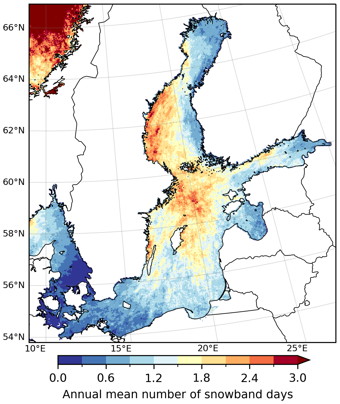
Figure 5 Annual mean number of snowband days in 1998–2018 in HCLIM detected by using the refined snowband criteria (see criteria in Table 1). Snowband day in each grid box is defined here as a day during which all the criteria were fulfilled at least once.

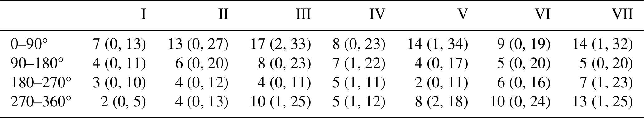
In Fig. 6, the snowband days in each grid box from Fig. 5 were further classified into four wind sectors based on the wind direction at the 900 hPa level. Figure 6 indicates that snowband days over the Baltic Sea are most common when the wind has an easterly component (winds are from 0–180°, Fig. 6a–b). Winds from 0–180° favour the occurrence of snowband days particularly near the eastern coast of Sweden and southern coast of Finland (Fig. 6a–b). Snowband days in these regions typically occur when northerly-to-southeasterly winds transport cold Arctic or continental air masses over the Baltic Sea, thereby increasing the vertical temperature difference between the surface and the overlying airmass, and provide a long fetch over open water. When the low-level wind has a westerly component (winds are from 180–360°, Fig. 6c–d) the number of snowband days in all regions, except for the southern and southeastern Baltic Sea, is smaller. With these wind directions, snowband days are most common in the Northern Baltic Proper, Eastern Gotland Basin and Bay of Gdansk (Fig. 6c–d). The annual number of snowband days detected in seven subregions of the Baltic Sea (see subregions in Fig. 6a) in 1998–2018 is collected into Table 3. Note that in Table 3, the size of each subregion varies and therefore the numbers between regions are not directly comparable.

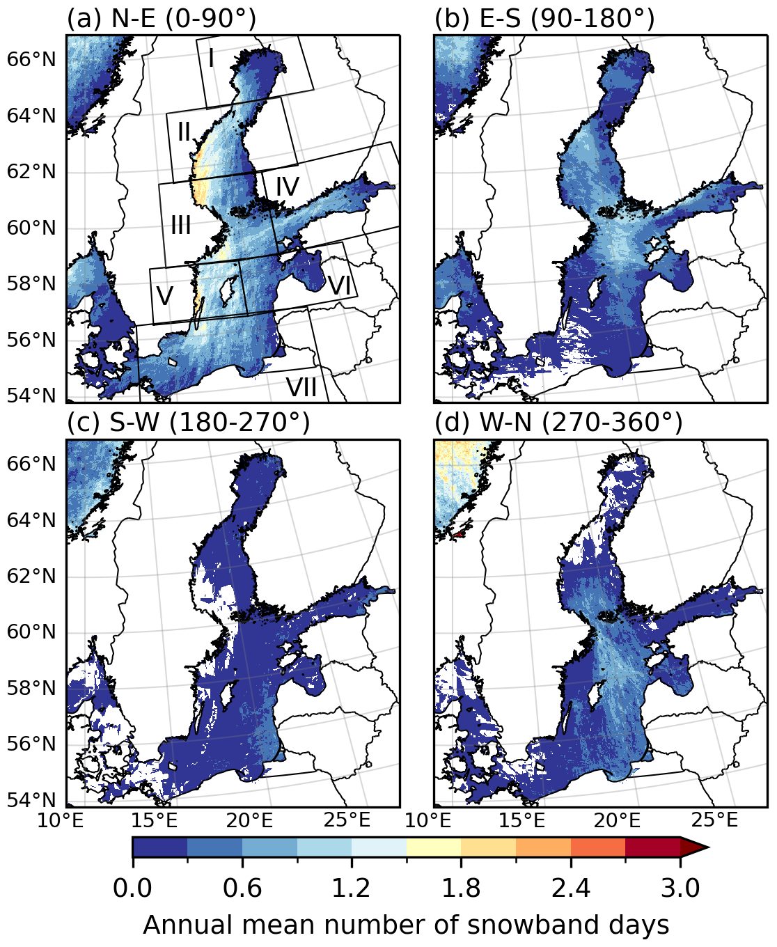
Figure 6 As in Fig. 5, but with an additional criterion for the wind direction at the 900 hPa level between (a) 0–90°, (b) 90–180°, (c) 180–270° and (d) 270–360°. The subregions presented in Table 3 and Fig. 8 are marked in (a).

Table 3 The average, and minimum and maximum (in brackets), annual number of snowband days in HCLIM in 1998–2018 in the subregions shown in Fig. 6. The snowband days are detected using the refined snowband criteria but with an additional criterion for the wind direction at the 900 hPa level between 0–90°, 90–180°, 180–270° or 270–360°. Snowband day is defined here as a day during which all the criteria are fulfilled in at least one grid box at least once per day somewhere in the subregion.

Snowband days over the Baltic Sea area occur mainly between October and March (Fig. 7b–g), however, the seasonal cycle varies between different regions. Over the northernmost Baltic Sea, snowband days occur primarily between October and December (Fig. 7b–d). Southward, over the Bothnian Sea, Gulf of Finland and Northern Baltic Proper, the average season is between November and February (Fig. 7c–f). The southern parts of the Baltic Sea typically experience snowband days slightly later, between December and March (Fig. 7d–g). The seasonal cycle of snowband days is governed, to a large part, by the seasonal cycle in air and sea-surface temperatures as sea-effect snowfall cannot occur if the sea is covered in ice or the airmass is too warm. Figure 7 shows that the seasonal cycle in mean sea ice extent (calculated using the threshold value of 15 % sea ice fraction, see e.g. Eisenman, 2010) is generally in line with the seasonal cycle in the number of snowband days. However, there is considerable inter-annual variability in the sea-ice extent (see Vihma and Haapala, 2009, and references therein) which is also the case for the number of snowband days (Tables 2 and 3). Namely, during warmer winters, the sea ice may cover only parts of the Bothnian Bay, Bothnian Sea and Gulf of Finland whereas in severe winters sea ice may extend to large parts of the Eastern Gotland Basin (Vihma and Haapala, 2009).

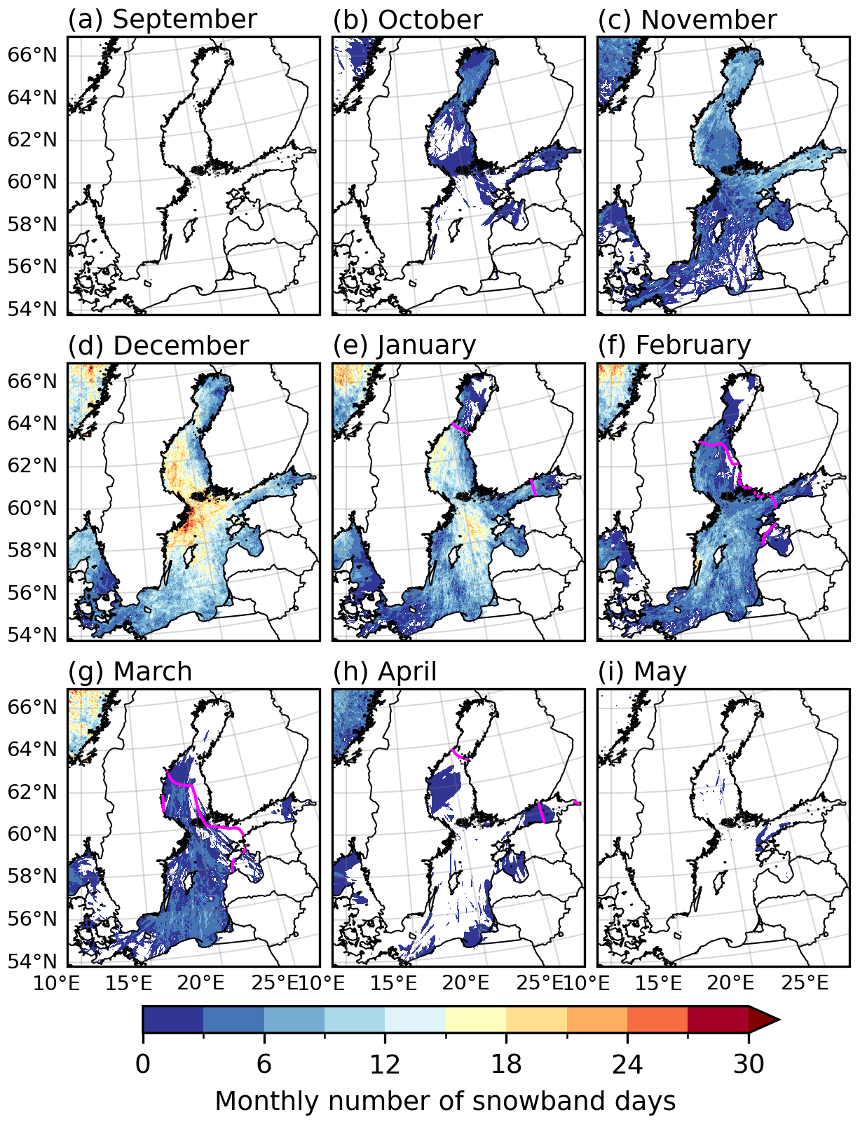
Figure 7 As in Fig. 5, but for the total monthly number of snowband days. Purple line indicates the mean sea ice extent in HCLIM.

The number of detected snowband days is somewhat sensitive to the number of criteria and the thresholds used in the detection method (OLS2020, OLS2023). When the looser set of criteria (see Table 1) is used, the number of detected days is higher (Fig. A3) compared to the refined criteria (Fig. 5), however, the spatial distribution in both cases is similar. This confirms that the general distribution of snowband days is primarily determined by the distribution of sea-surface temperature and the vertical temperature difference between the sea-surface and the lower troposphere. Lastly, the snowfall threshold used in this study was set to be quite high. When the 3 hourly snowfall threshold in the refined snowband criteria is lower (higher), the number of detected cases is higher (lower), but the spatial distribution is generally similar (Fig. A4).

3.4 Snowfall on snowband days

The most impactful snowbands are those that move over land. In order to estimate the snowfall distribution associated with snowband days over land and to identify the areas that receive most snowfall, we divide the Baltic Sea area into seven subregions and study the mean daily snowfall calculated from snowband days occurring in each region (Fig. 8). The snowband days are divided into four wind sectors as in Fig. 6 since the prevailing wind direction determines the movement direction of snowbands and the potential impact region over the coastline. Figure 8 shows that the mean daily snowfall on snowband days is generally higher over land than over the sea. In downwind facing coastlines over land, snowfall is generally most intense near the coastline. The highest mean amounts (up to 2.7 mm d⁻¹ in liquid water equivalent) occur over the eastern coast of Sweden with winds from 90–180° (Fig. 8b).

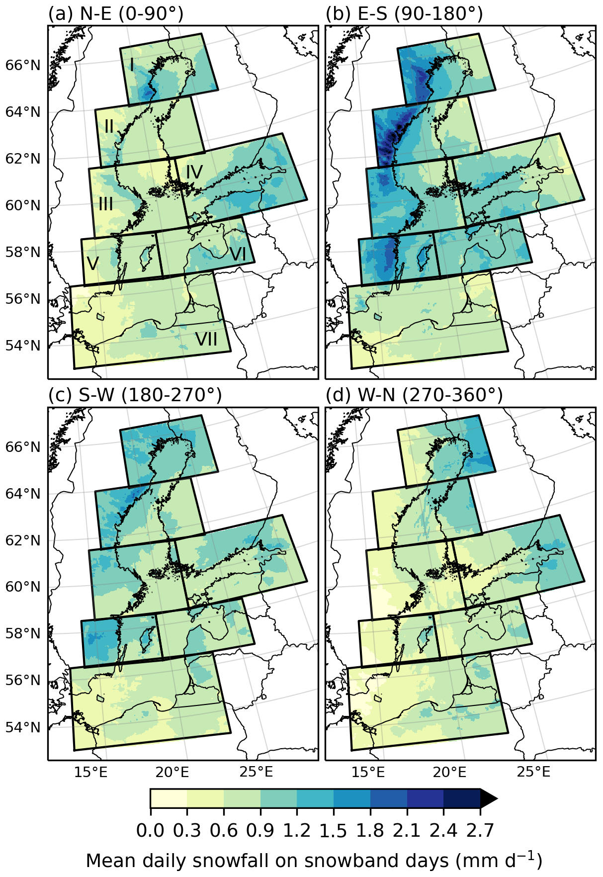
Figure 8 Mean daily snowfall on snowband days in seven subregions of the Baltic Sea area. The snowband days are detected using the refined snowband criteria but with an additional criterion for the 900 hPa-level wind direction between (a) 0–90°, (b) 90–180°, (c) 180–270° or (d) 270–360°. Snowband day in each subregion is defined here as a day during which all the criteria were fulfilled in at least one grid box at least once per day somewhere in the subregion.

Note that not all snowbands in Fig. 8 drift over land and that some of the detected days likely include also non-convective snowfall occurring on snowband days. In Fig. 8, attention should be focused mainly on the coastlines that are downwind of the prevailing wind direction. Considerable snow amounts are seen for example over the eastern coast of Sweden over land in region V with winds from 180–270°, which include winds directed away from the coastline and that generally do not favor snowbands in those regions (Fig. 6c and Table 3). The snowfall may have been sampled due to an approaching low-level system with large-scale snowfall occurring before or after a snowband was detected in the subregion. On the other hand, convective snowbands may also be embedded within low-pressure related large-scale snowfall (see e.g. Saarikivi, 1989). Thus, the daily total snow amount on snowband days can often be a combination of both localized intense convective snowfall and weaker large-scale snowfall.

3.5 Sea-effect snowfall in eastern Sweden, southern Finland and northern Poland

Three regions with numerous snowband days in Fig. 5 and high mean snowfall (Fig. 8) are chosen for a more detailed investigation. Figure 9 shows the 98th percentile of daily snowfall and the number of days with daily snowfall exceeding 5 mm d⁻¹ on snowband days over the northeastern coast of Sweden (Fig. 9a–b), southern coast of Finland (Fig. 9c–d) and northern coast of Poland (Fig. 9e–f). Note that in Fig. 9, low-level winds have been restricted to be towards the coastline to focus on events that likely result in snowfall over land. Figure 9 shows that Finland and Poland generally experience more moderate (98th percentile is up to 5–6 mm d⁻¹ in liquid water equivalent) snowfall than Sweden (over 8 mm d⁻¹). The same holds true also for the number of days with snowfall exceeding 5 mm d⁻¹, namely, some regions in the Swedish coastline experience up to 25 d whereas Finland and Poland experience only up to ten during the 21 year long time period.

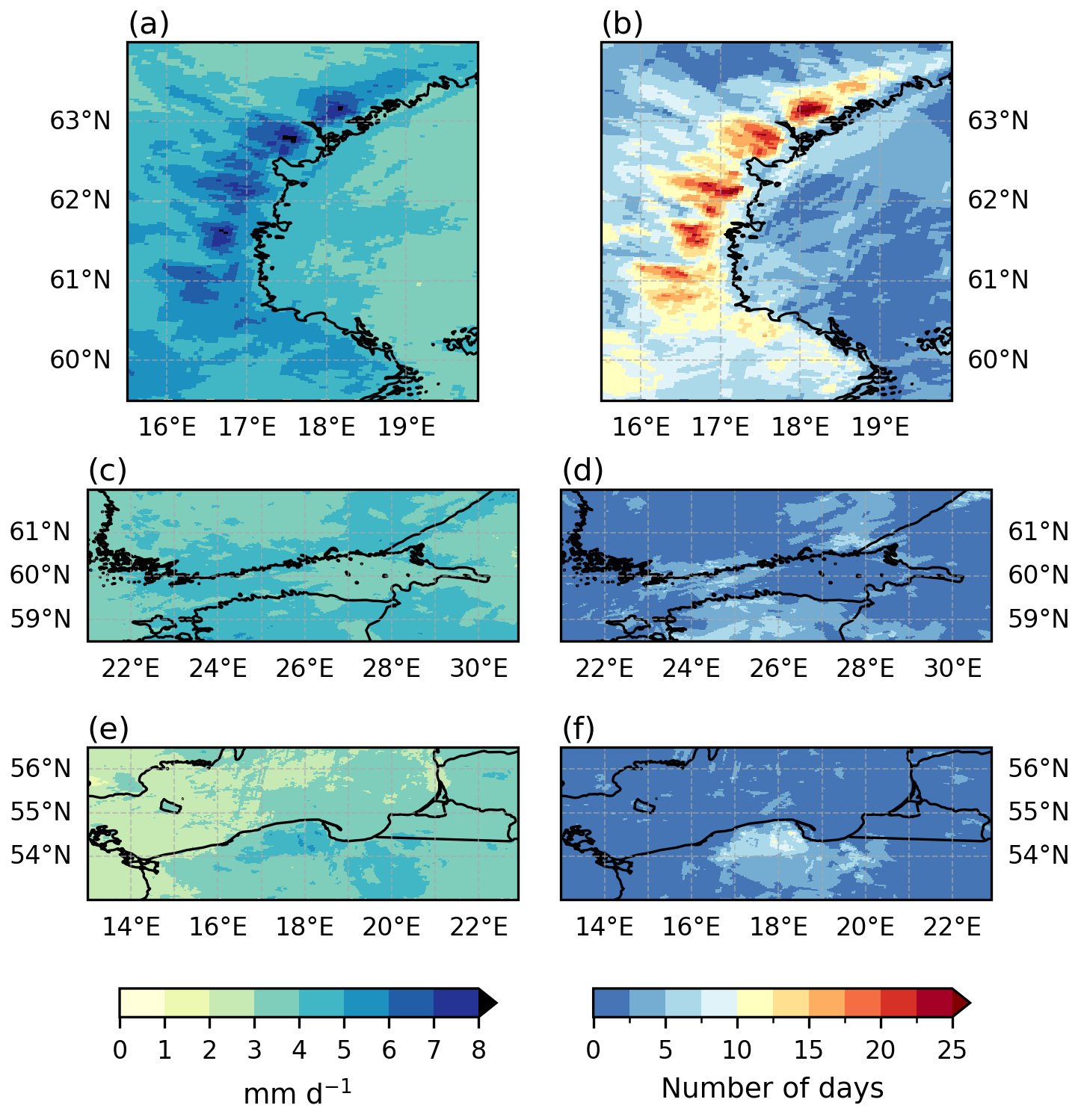
Figure 9 98th percentile of daily snowfall on snowband days (left column) and number of days with snowfall exceeding 5 mm d⁻¹ on snowband days (right column) in the three subregions shown in Fig. 1. Snowband day in each subregion is defined here as a day during which all the refined snowband criteria (see Table 1) were fulfilled, and the wind direction at the 900 hPa level was (a–b) 350–360° or 0–140°, (c–d) 90–255° and (e–f) 280–360° or 0–80°, in at least one grid box at least once somewhere in the subregion.

Figure A2 and previous studies (see e.g. OLS2023 and Bednorz et al., 2022) have shown that sea-effect snowfall systems over the Baltic Sea can occur under a variety of large-scale weather patterns. A key requirement is a flow that advects cold air over the sea. Figure 10 shows the composite mean geopotential height at the 500 hPa level and mean sea level pressure (values at 12:00 UTC) for snowband days in the three regions of Fig. 9. We note that as composites do not capture the full variability of large-scale weather conditions, these results should be interpreted with caution. For snowbands potentially affecting the eastern coast of Sweden, the mean large-scale weather pattern comprises an upper-level trough and low-level low-pressure system over the southern half of the Baltic Sea, producing a northeasterly mean low-level flow over the Bothnian Sea (Fig. 10a). Snowbands drifting over southern Finland from the Gulf of Finland show a somewhat similar configuration, with low-level southerly-to-southeasterly winds in that region (Fig. 10b). In contrast, snowbands forming near the northern coast of Poland are associated with somewhat higher mean sea-level pressure, a low-pressure area over eastern Baltic countries and mean low-level flow from the north, guiding cold air into the region (Fig. 10c).

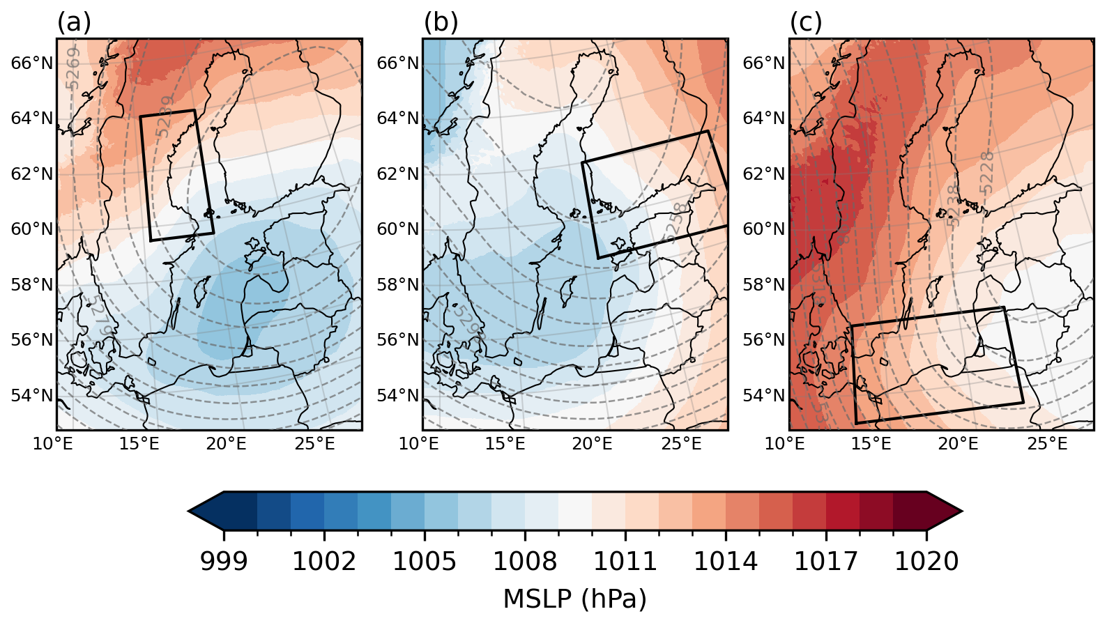
Figure 10 Composite mean geopotential height at the 500 hPa level (gpm, contours, contours shown every 10 gpm) and mean sea level pressure (hPa, color shading) associated with snowband days in the three subregions shown in Figs. 1 and 9. Snowband day in each subregion is defined here as a day during which all the refined snowband criteria (see Table 1) were fulfilled, and the wind direction at the 900 hPa level was (a) 350–360° or 0–140°, (b) 90–255° and (c) 280–360° or 0–80°, in at least one grid box at least once somewhere in the subregion.

4 Discussion

In this study, snowband days over the Baltic Sea area occur most frequently near the east coast of Sweden, over the Gulf of Finland and Northern Baltic Proper (Fig. 5). Snowband days are most prevalent when the low-level winds have an easterly component (i.e. wind direction at the 900 hPa level is between 0 and 180°, Fig. 6a–b, Table 3). The HCLIM-based snowband climatology resembles the 11 year climatology of snowbands for Sweden, being simulated with another, coarser-resolution, regional climate model by JEW2017. They showed that when the low-level wind was from 0–90°, hotspots for precipitation on days with favourable conditions for convective snowbands typically occurred over land in the Swedish coast of the Bothnian Sea and Western Gotland Basin, as well as in Gotland (see Fig. 4 in JEW2017). In the majority of those regions, mean daily snowfall was between 1 and 2 mm d⁻¹ (JEW2017). Local maxima in mean daily snowfall on snowband days (mean daily snowfall between roughly 0.9 and 2.1 mm d⁻¹) are also seen in the above mentioned regions in the current study (Fig. 8a–b). Furthermore, although less frequent, snowbands in HCLIM are also detected over the southern Baltic Sea (Fig. 5), where they are mostly associated with northwesterly-to-northeasterly winds (Fig. 6a and d) and typically occur between November and March (Fig. 7). This is consistent with the findings of Bednorz et al. (2022), who documented typical conditions linked to 25 extreme snowfall events occurring over northern Poland. Their extreme cases (that led to observed snow depth increase of at least 20 cm within two days) occurred between November and February, typically under a northeasterly circulation in the lower troposphere over warm sea water, driven by a low-pressure area in eastern Europe. In the current study, a local maximum in daily snowfall (98th percentile between 4 and 5 mm d⁻¹ in liquid water equivalent) on snowband days with winds towards the Polish coastline was found near the northern coast of Poland (Fig. 9e–f).

The snowband day climatology near the Finnish coastline also shares several similarities with the previously defined climatology of OLS2020 and OLS2023. When the criteria of OLS2023 were applied to HCLIM data, the annual mean number and monthly distribution of snowband days in Finland closely resembled those shown by OLS2023 (Table 2 and Fig. 2). Snowband days in HCLIM occurred most frequently along the southern coast of Finland in S, consistent with the main hotspots reported in OLS2023. A notable difference between the current study, OLS2020 and OLS2023, however, was seen in the location of the most favourable region for snowband occurrence. While OLS2020 and OLS2023 found that the most favourable region for snowband occurrence was near the western coast of Finland (region W) during southerly-to-westerly winds, this maximum in occurrence frequency is absent in HCLIM (Fig. 3, Fig. 6). In fact, winds with a westerly component were found to be the least favourable for snowband occurrence across the northern Baltic Sea in HCLIM (Fig. 6c–d).

The reason for this discrepancy is not fully understood. On one hand, HCLIM has a superior spatial resolution (3 km), uses non-hydrostatic dynamics, and explicitly resolves deep convection. Even though the resolved convection and high resolution likely bring more added value for summer than for winter convection, they are beneficial also in the latter, allowing HCLIM to represent many convective circulations more accurately than the datasets used by OLS2020 and OLS2023. Namely, OLS2020 used regional climate model data with 11 km resolution and parameterized deep convection, whereas OLS2023 used the ERA5 reanalysis data at 31 km resolution, which exceeds the size of the smallest sea-effect snowfall systems. This leads to uncertainty in the representativeness of snowbands in those datasets. For example, over the Great Lakes area, Notaro et al. (2015); Lucas-Picher et al. (2017) have shown that climate models with grid spacings larger than 10 km were not able to accurately represent all lake-effect snowfall events (see also Lucas-Picher et al., 2021). On the other hand, OLS2023 showed that ERA5 was able to successfully capture past well known cases of sea-effect snowfall.

Four case studies from the northern Baltic Sea revealed that HCLIM was able to simulate past high-impact snowbands well and the sea-effect snowfall detection method captured the events. The case studies and comparison to the previous climatology by OLS2023 support the utility of HCLIM and the refined snowband criteria to identify the general occurrence distribution of snowband days and areas most at risk from convective snowfall over the Baltic Sea area. However, it should be kept in mind that the detection method does not explicitly find convective precipitation and, instead, is based on finding days with considerable snowfall and environmental conditions that favor the occurrence of snowbands. It is therefore possible that some of the detected snowband days that form the snowband day climatology did not actually involve convective precipitation forced by the sea-effect. On the other hand, some cases may be undetected if the criteria used by the detection method are too strict.

5 Conclusions

In this study, we use the convection-permitting HCLIM climate model data at 3 km horizontal and 3 h temporal resolution to study the long-term occurrence of snowband days over the Baltic Sea area in 1998–2018. To accomplish this goal, we utilize a refined sea-effect snowfall detection method that finds the grid boxes and time steps with considerable snowfall (3 hourly snowfall over 0.5 mm) and environmental conditions known to be favourable for the occurrence of snowbands (see criteria in Table 1).

According to HCLIM, snowband days (i.e. days when all the refined snowband criteria are fulfilled at least once) are most frequent near the east coast of Sweden, southern coast of Finland and between Sweden and Estonia (up to a few snowband days per year in a 3 km×3 km area) and when the low-level wind has an easterly component. Over the northern Baltic Sea, the snowband season typically begins in October and ends in February. Over the southern Baltic Sea, snowband days are favoured by low-level winds having a northerly component and occur typically between December and March. A more detailed summary of the key findings for different regions of the Baltic Sea is as follows:

• Gulf of Bothnia between Sweden and Finland: Snowband days typically occur in October–January over the Bothnian Bay in the north and in November–February over the Bothnian Sea in the south, most frequently near the eastern coast of Sweden, and with low-level winds from 0–180°. On snowband days, mean daily snowfall is highest near the Swedish coastline. Daily snowfall over 8 mm d⁻¹ (98th percentile, liquid water equivalent) is seen near Sweden over the Bothnian Sea when low-level winds are towards the coastline.

• Gulf of Finland between Finland and Estonia: Most snowband days occur between November and February and with low-level winds from 0–180°. Considerably fewer snowband days are seen with westerly winds. On snowband days with low-level winds towards the Finnish coastline, daily snowfall is over 6 mm d⁻¹ (98th percentile, liquid water equivalent) near the coastline.

• Northern Baltic Proper between Sweden, Finland and Estonia: Snowband days are detected mainly between November and March, peaking between December and January and occur mainly with low-level winds from 0–180° and 270–360°.

• Southern Baltic Sea: Snowband days are most common near the east coast of Sweden and near the coast of Poland and Lithuania. The average season spans December–March. Low-level winds from 0–90° favor snowband days near Sweden. Over the southernmost Baltic Sea near the Bay of Gdansk, snowband days occur mostly with winds from 0–90° and 270–360°.

Four case studies of verified past sea-effect snowfall systems in the Baltic Sea area show that HCLIM, with reanalysis data used for lateral boundary conditions, is able to simulate the location and morphology of the snowbands surprisingly well. The detection method, with the refined snowband criteria, was able to capture snowband days in the correct general impact areas. Furthermore, the long-term occurrence distribution presented in this study in generally in line with past regional climatologies presented in other studies. This supports the utility of the kilometer-scale regional climate model HCLIM, that has previously been shown to lead to considerable added value in the representation of summertime extreme precipitation, also in studies of past and future distributions of convective snowfall in northern Europe.

We note that the methodology used to construct the snowband day climatology has some limitations. The detection method does not explicitly seek to identify convective precipitation. Instead, the environmental conditions need to fit the criteria defined in previous studies of sea-effect snowfall for the snow system to be included in the snowband day climatology. The criteria consist of quantitative thresholds for different meteorological parameters, which the number of detected days is sensitive to. Therefore, the method might miss some snowbands if the criteria are too strict, or capture non-convective snowfall if the criteria are too loose. Furthermore, although HCLIM represents previously defined snowband climatologies well, the model may contain uncertainties and biases that affect the long-term statistics. The 21 year period of investigation is rather short for studying long-term statistics, especially that of extremes. If a longer period, say 30 or 50 years, were used study the occurrence of snowband days, some local-scale differences with respect to our results may arise due to the natural spatial and temporal variability of the snowbands.

The number of detected snowband days was shown to be sensitive to the number of criteria, however, the general characteristics of the occurrence distribution remained largely unchanged. This suggests that the spatial distribution of snowband days is primarily determined by the distribution of sea-surface temperature and the vertical temperature difference between the sea-surface and the lower troposphere. Understanding how climate change affects the extent and annual cycle of sea ice – as well as the co-occurrence of ice-free sea and cold lower-tropospheric air masses – can thus provide valuable insights into how the general characteristics and spatial distribution of sea-effect snowfall may change in the future.

This study presents, for the first time, the climatology of snowbands environments over the full Baltic Sea region. Such a climatology is important as it can be used to identify areas most at risk from sea-effect snowfall and thereby support the planning and implementation of climate adaptation measures, while also providing useful context for weather-related decision-making. The results form the fundamental basis for studying impacts of future climate change on the occurrence, frequency and intensity of sea-effect snowfall in northern Europe.

Appendix A

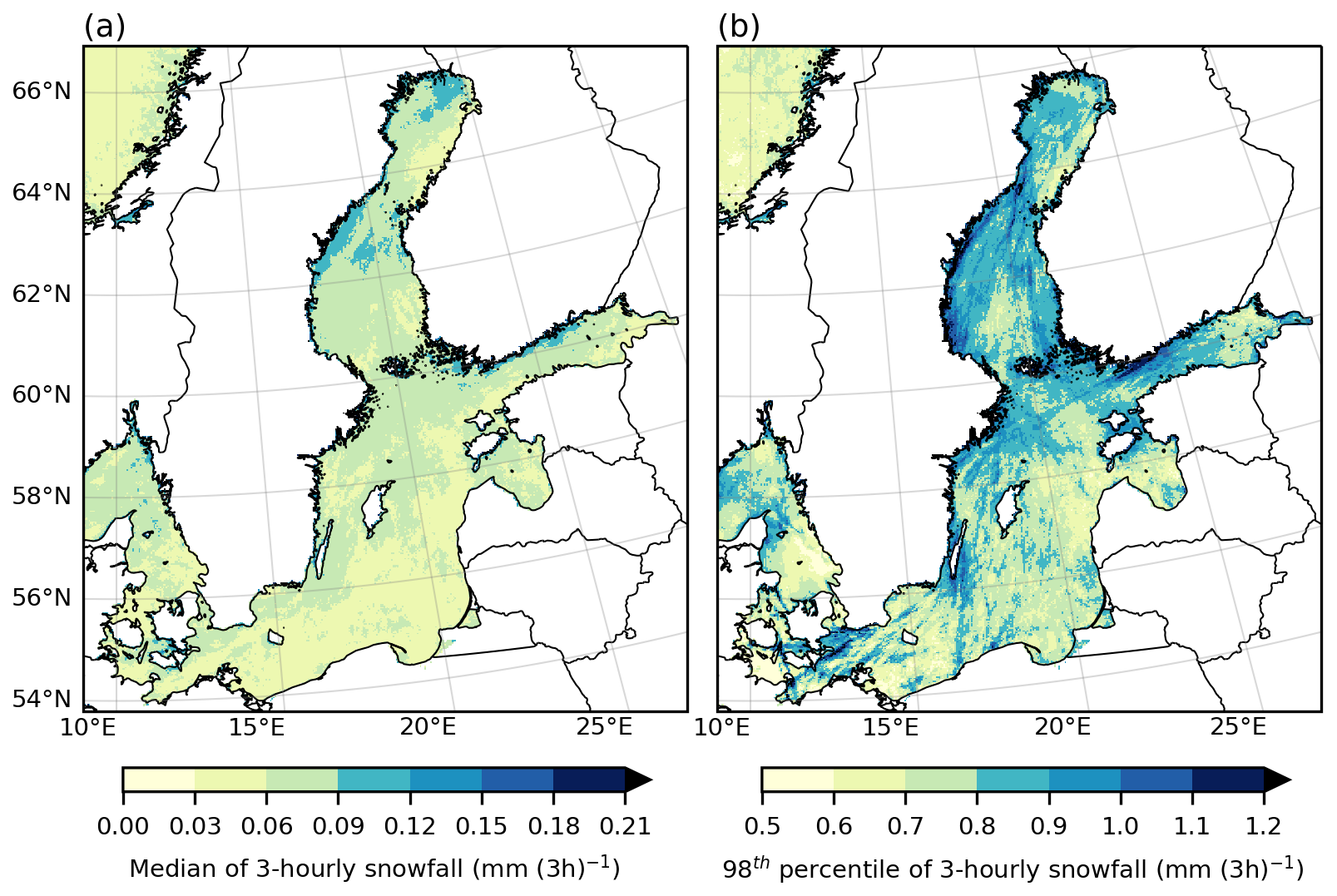
Figure A1 (a) Median and (b) 98th percentile of 3 hourly snowfall in 1998–2018 in HCLIM. The median and the 98th percentile of snowfall is calculated from time steps when all the refined criteria shown in Table 1 (except the criterion for 3 hourly snowfall exceeding 0.5 mm) are fulfilled and at least some snowfall occurs (i.e. 3 hourly snowfall rate exceeds 0.01 mm (3 h)⁻¹).

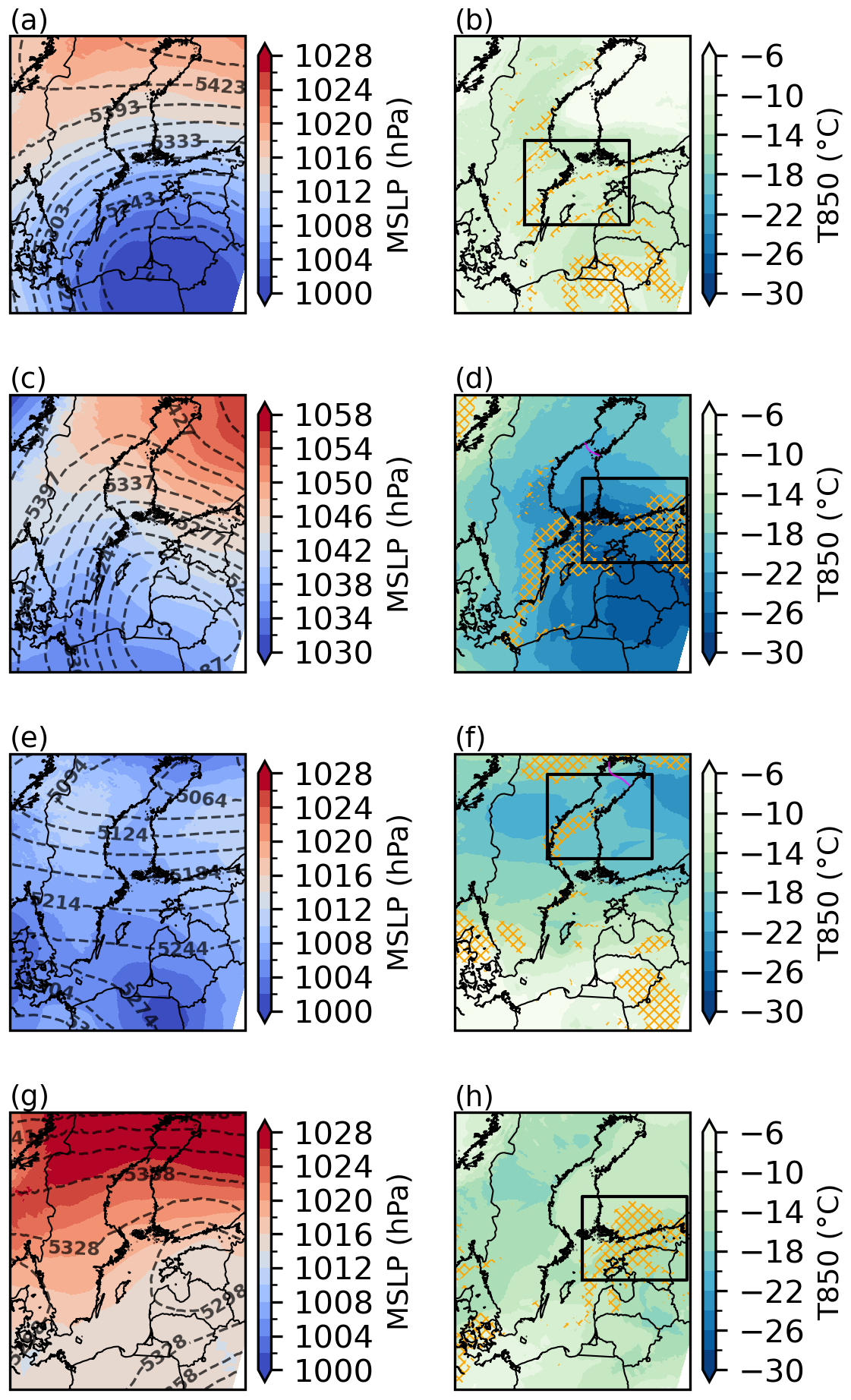
Figure A2 Geopotential height at the 500 hPa level (gpm, contours) and mean sea level pressure (hPa, color shading, first column), as well as temperature at the 850 hPa level (°C, color shading), occurrence of snowfall exceeding 0.1 mm (3 h)⁻¹ (orange rasters) and sea ice extent (magenta contour, second column) in HCLIM on 13 November 2007 at 12:00 UTC in (a–b), on 2 February 2012 at 12:00 UTC in (c–d), on 9 January 2016 at 00:00 UTC in (e–f), and on 8 November 2016 at 12:00 UTC (g–h).

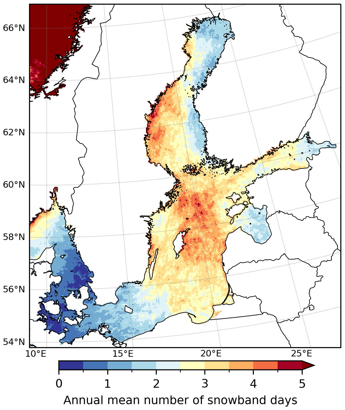
Figure A3 Annual mean number of snowband days in 1998–2018 in HCLIM detected by using the loose criteria (see criteria in Table 1). Snowband day in each grid box is defined here as a day during which all the criteria were fulfilled at least once.

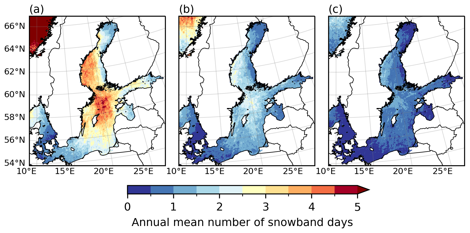
Figure A4 Annual mean number of snowband days in 1998–2018 in HCLIM detected by using the refined snowband criteria, but with the threshold for 3 hourly snowfall being (a) 0.3 mm (3 h)⁻¹, (b) 0.5 mm (3 h)⁻¹ and (c) 0.8 mm (3 h)⁻¹. Snowband day in each grid box is defined here as a day during which all the criteria were fulfilled at least once.