Transient flow patterns of an annular-like stratospheric polar vortex

A two-component study is undertaken of sub-planetary scale flow features associated with the wintertime polar-night vortex at upper-stratospheric levels. First, case studies based upon reanalysis data are presented to illustrate the scale, structure, evolution and dynamics of the features potential vorticity in three disparate flow settings along with signatures of some accompanying flow, thermal, and constituent variables. The features are shown to be present near the periphery of the vortex and are associated with the vortex's predilection to develop a structure akin to an annular-like band of enhanced potential vorticity. Second, theoretical considerations and numerical model simulations of perturbations of an annular band of enhanced absolute vorticity using a non-divergent barotropic model on a polar β-plane yield results consistent both with the occurrence and character of the observed sub-planetary scale features, and with the rapid reconfiguration of the band when subject to a planetary scale wave perturbation. The latter result suggests that that the break-up of the polar vortex at stratopause-levels can be facilitated by the synergetic combination of strong planetary-scale Rossby-wave forcing from below acting upon the vortex's annular potential vorticity band.

1 Introduction

The general form of wintertime stratospheric polar vortex (SPV) is well established (see e.g. Waugh and Polvani, 2010; Schoeberl and Newman, 2015; Butchart, 2022). It extends from the lower stratosphere at ∼15 km to well beyond the stratopause at ∼50 km, attains a maximum wind strength often greater than 120 m s⁻¹ at stratopause levels, and is characterized in the stratosphere by an inner cold core driven primarily by the lack of ozone-related radiative heating during the polar night.

On quasi-horizontal or isentropic surfaces, the SPV's lateral “edge” has been defined in various ways (Waugh et al., 2016; Manney et al., 2021). Kinematically it has been associated with the iso-line demarking the strongest wind strength (Waugh et al., 2016) or the maximum streamline density (Harvey et al., 2002; Harvey et al., 2009), cartographically as a feature-based configuration (Serra et al., 2017; Lawrence and Manney, 2018), and dynamically as the zone of sharp lateral PV gradient (Butchart and Remsberg, 1986; Manney et al., 2022; Nash et al., 1996). The latter definition arises from regarding the vortex's lateral configuration as an inner core of high potential vorticity (PV) encased by a narrow zone of strong PV gradient that is itself encircled by broad and well-mixed surf zone of lower PV (McIntyre and Palmer, 1984). The adoption of one or another of the above criteria to define the vortex's periphery will depend upon its practical utility or its interpretative value for the specific purpose in hand.

The present study is geared to examining the sub-planetary and finer-scaled flow features that are contiguous to, or related to, the structure of the SPV's periphery, and to this end we utilize the PV perspective (Hoskins et al., 1985). The study is framed around the postulate that a, possibly fragmented, annulus of enhanced PV (i.e. a maximum in the across-jet distribution of the PV) can exist near the periphery. This assertion is rendered plausible by two factors. First, a strong laterally confined jet with a relative vorticity maximum (say, ζ_max) located at a co-latitude χ (<30°) on the vortex's poleward side would connote a maximum of absolute vorticity provided (${\mathit{\zeta }}_{\max }/\mathrm{2}\mathrm{\Omega }$) $>\mathrm{1}/\mathrm{2}{\mathit{\chi }}^{\mathrm{2}}$, and this inequality is readily satisfied (often by an order of magnitude) in the upper stratosphere. This in turn would connote a PV maximum (sic annulus of enhanced PV) if the variation of the stratification on an isentropic surface within the vortex is not comparably large. Second, the presence of such an annular structure on an isentropic surface is a necessary criterion for instability of axisymmetric quasi-geostrophic stratospheric flow (Charney and Stern, 1962), and the realization of the instability could result in a fragmented annulus.

The probable existence of such an annular structure in the polar stratosphere has long been recognized (Hartmann, 1983), and indeed a balanced flow response to a radiative equilibrium (Leovy, 1964) or radiatively determined (Shine, 1987) stratospheric state would possess such a maximum. Such a feature has also been detected in other planetary atmospheres (e.g. Sharkey et al., 2021; Shultis et al., 2025) and is often a feature in the vicinity of the hurricane's eyewall (Schubert et al., 2018). Moreover, Davies and Sprenger (2024) – hereafter denoted DS24 – drew attention to flow features at stratopause elevations that are akin to that of a fragmented annulus.

An annular structure of enhanced PV would be embedded within an SPV that itself exhibits a distinct life cycle (Lu et al., 2021), and marked inter-annual variations (Butchart, 2022; Rao et al., 2024) particularly those related to the occurrence and aftermath of a Sudden Stratospheric Warming (Baldwin et al., 2021). This poses questions as to whether the annular structure or its fragmented counterpart is present at all phases of the life cycle, and what role (if any) it plays in the development of Sudden Stratospheric Warming (SSW) events that have themselves been pointedly linked to a variety of mechanisms and preconditioned states deemed to be more amenable to engendering such events (Plumb, 1981; Frederiksen, 1982; Smith, 1992; Matthewman and Esler, 2011; de la Camara et al., 2017; Lawrence and Manney, 2020; Yessimbet et al., 2022).

Again, the annulus occupies the same spatial domain as two classes of shorter-term phenomena, and questions arise regarding the extent of their inter-dependence. One class can be viewed as intrinsic natural modes confined to, and governed by the structure of, the SPV itself such as planetary-scale zonally propagating waves (Venne and Stanford, 1979; Randel and Lait, 1991), smaller scale zonally propagating waves and synoptic-scale features (Harvey et al., 2002; Lu et al., 2021). The second class comprise planetary-scale Rossby waves (PRWs) (see e.g. Hitchcock and Haynes, 2016) and short-term smaller-scale gravity waves (GW) (see e.g. Holton and Alexander, 2000; Eichinger et al., 2020) both of which propagate upward from lower elevations and can break on attaining large amplitude. Both are influenced by the SPVs structure, and the PRWs tend to break in the mid-to-upper stratosphere and the GWs at even higher elevations. On breaking they can heavily modulate the SPV's structure. Indeed, breaking PRWs (Hitchman and Huesmann, 2007; Greer et al., 2013) strip PV filaments off the vortex edge, create the surf zone (McIntyre and Palmer, 1984), and are endemic to the occurrence of SSW events (Martius et al., 2009). Likewise breaking gravity waves can serve as a drag (GWD) reducing the strength of the SPV's jet.

In this study attention is focused on the presence, role and dynamics of a PV annulus and/or its fragmented counterpart in the wintertime upper stratosphere. It is set against the backcloth of the series of questions posed above, and it has observational and theoretical components. For the observational component, illustrative case studies pertaining to the SPV's annular structure are presented for three different winter settings. For each case attention is drawn to the structure, temporal evolution, and dynamical character of the realized transient sub-planetary and planetary scale flow features. The three cases comprise: (i) a mildly perturbed mid-winter vortex in the Northern Hemisphere, (ii) a comparatively undisturbed early winter vortex in the SH, and (iii) a highly disturbed NH vortex in mid-February associated with a developing SSW.

The theoretical component is prompted by noting that the observationally detected features (DS24) bear comparison with the break-up of a barotropic jet-like flow. The ready inference that a jet-like structure might satisfy a necessary condition for barotropic instability has spawned a fleet of studies for basic states akin to that of: the SPV's jet and the circumpolar jets of other planetary atmospheres (see for example, Pfister, 1979; Davies, 1981; Hartmann, 1983; Michaelangeli and Zurek, 1987; Manney et al., 1988; Seviour et al., 2017; Mitchell et al., 2021; Waugh, 2023); the hurricane's eyewall (Schubert et al., 2018); and the inner region of extratropical cyclones (Leutwyler and Schär, 2019). Key dimensionless parameters that govern the dynamics of these other systems can differ substantially from those that pertain to the stratosphere's polar night jet, but herein we consider only flow settings representative of the SPV. The strategy adopted here is to select an idealized theoretical model capable of capturing the essence of rapidly growing wave patterns of a barotropic model for flow settings akin to that of a deep undisturbed SPV. The specific objective is not to replicate (or contrast) the results with that of the earlier studies, but rather to seek further basic understanding of, and insight upon, the dynamics of the observed features.

Both components are foreshadowed by the recognition that the presence of an annular PV feature in the upper stratosphere would influence the character of in-situ generated phenomena and of waves propagating into the domain. For example, a change in the SPV's structure modifies its transmissivity to upward propagating waves (Hitchcock and Haynes, 2016). The strong positive PV gradient on the outer side of the annulus constitutes a columnary shaft that favours vertical PRW propagation (Abatzoglou and Magnusdottir, 2007). Contrariwise, the negative PV gradient on its inner side would inhibit the propagation into the vortex core, and thereby in principle help isolate the core from external effects. It is pertinent to note that this “shielding of the vortex core” associated with the PV gradients contrasts markedly with the dynamics at the counterpart tropopause-level sharp PV gradient (and accompanying jet stream) located at the break in the mid-latitude extratropical tropopause (Appenzeller and Davies, 1992).

The paper is arranged as follows. Section 2 sets out the observational case studies. Section 3 sets out the theoretical results derived using an idealized barotropic model to study the dynamics of both small and finite amplitude perturbations of an SPV-like basic state. In a final section further remarks are made regarding the study's results and their possible implications.

2 Observed Flow Features

Three case-studies are presented with the objective of capturing the essence of transient flow features associated with an annular-like PV structure in the wintertime upper stratosphere.

2.1 Data

Consideration of the flow at stratopause and higher elevations using reanalysis data sets are subject to constraints arising from the decrease in the number and resolution of sampled meteorological variables and the shortcomings of the parent assimilation model at these elevations (see the overview in S-RIP, 2022). Nevertheless, Reanalysis fields have been utilized, albeit with caveats, to examine a range of upper stratospheric diagnostic studies. Moreover, DS24 showed examples of three Reanalysis data sets, viz. ERA-Interim (Dee et al., 2011), MERRA (Gelaro et al., 2017), and ERA-5 (Hersbach et al., 2020), capturing the same sub-planetary and synoptic-scale flow features.

Here, we proceed pragmatically, examine only levels at and below the prevailing stratopause and adopt the ERA-Interim data set. In Appendix A illustrations are provided of the overall similarity of this study's key PV patterns as captured by the ERA-Interim and MERRA2 Reanalysis data sets.

2.2 Diagnostic Analysis

The objective is to establish the existence, scale, structure, evolution and dynamics of the sub-planetary transient flow features. To this end the instantaneous scale and structure of the PV features is first illustrated at a vertical series of pressure-level charts. In addition, for two of the three case studies, we exploit the PV perspective (Hoskins et al., 1985) by displaying a time-sequence of displays on pertinent isentropic surfaces to capture: the time-development of the PV pattern; the possible Lagrangian-conservation of the PV of the individual features; and to assess the dynamics and possible instability of the flow. Note that the rapid vertical increase of the background PV can serve to diffuse/sharpen the equatorward edge of an annular feature on a pressure surface located above/below the stratopause in comparison to its structure on a contiguous isentropic surface.

Further insight is provided by examining aspects of the contemporaneous distribution, on pertinent pressure-level surfaces, of other flow variables including the relative vorticity, divergence, potential temperature, specific humidity and ozone mass mixing ratio. For each case study we present a summary of key features at the 10 mb level followed by examples of the structure and evolution of the flow at upper stratospheric levels for specific time windows.

2.3 Features of a Mid-winter SPV

The Boreal Winter of 2004–2005 was comparatively non-descript and there wasn't an SSW event. At the 10 mb level the time-latitude pattern of zonal mean velocity (Fig. 1a) increased almost monotonically to a maximum of ∼70 m s⁻¹ by 19 January and decreased almost uniformly thereafter. The corresponding time-longitude pattern of the meridional velocity at 60° N (Fig. 1b) shows evidence of a strong m=2 pattern by the middle of December. Its amplitude and phase remained comparatively constant for the remainder of the Winter although it transiently weakened and retrogressed in early January. The onset of the wave and the forementioned transient retrogression was accompanied by a relatively strong upward EP fluxes (not shown).

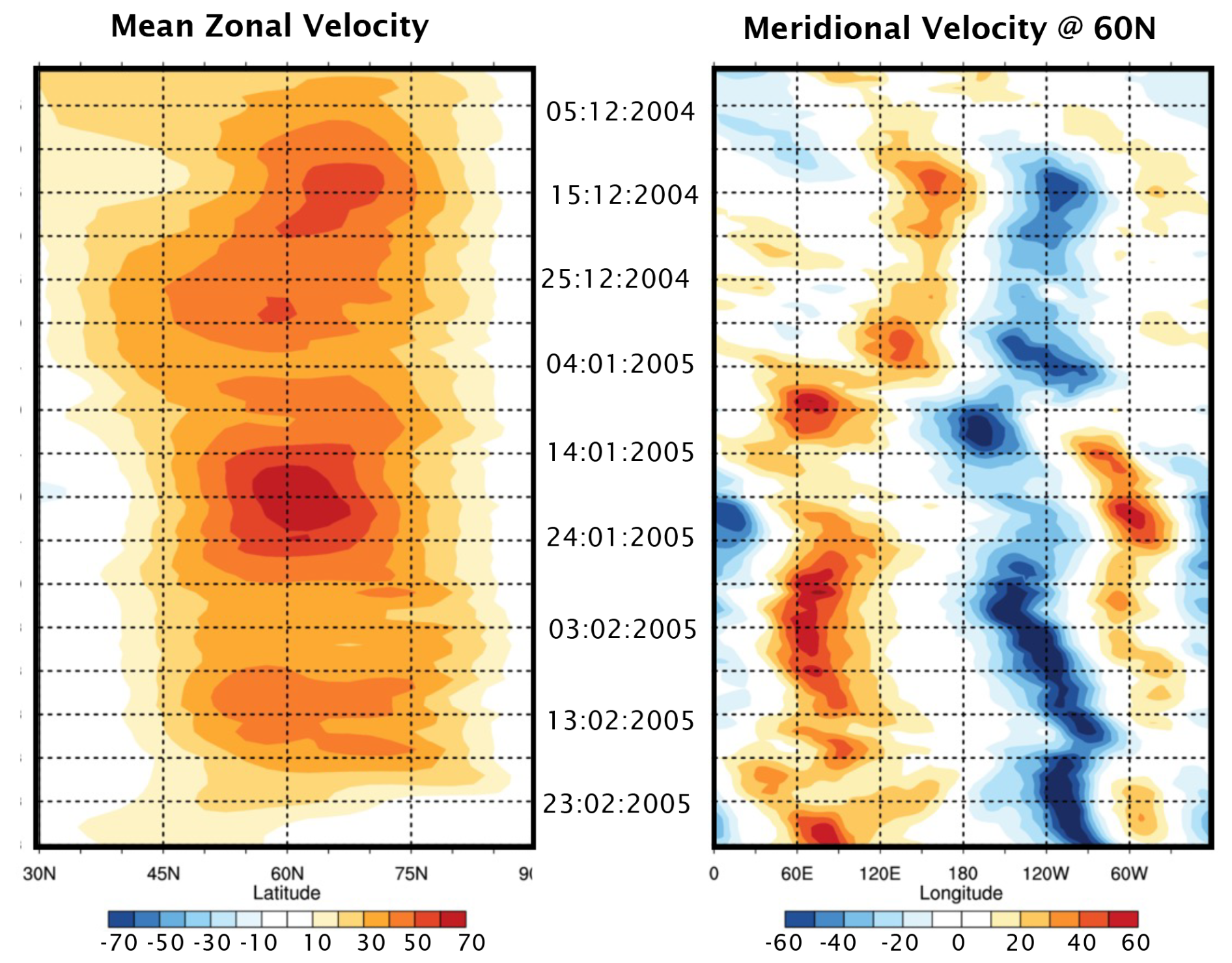
Figure 1 Panel (a) shows the zonal mean velocity as a function of latitude (30–90° N) at 10 hPa for the Boreal Winter of 2004–2005, and panel (b) depicts the meridional velocity field at 60° N at the same level for the same winter season (Based upon the NCEP/NCAR Reanalysis.).

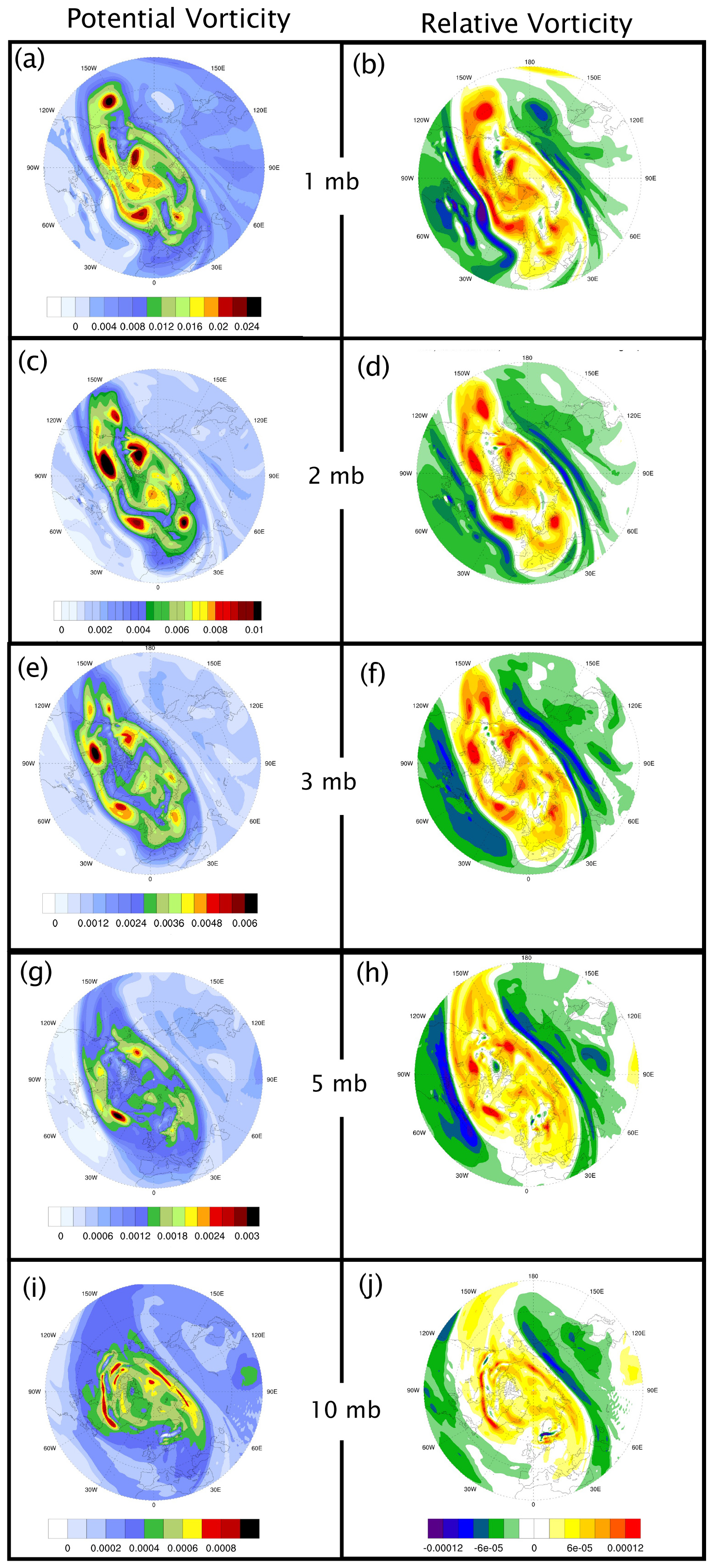
Figure 2 Depicted are polar stereographic projections poleward from 30° N of the PV in units of K m² kg⁻¹ s⁻¹ (left column) and the relative vorticity in units of s⁻¹ (right column) for 00:00Z 11 January 2005 on the 1, 2, 5 and 10 mb surfaces (Based upon the ERA-Interim Reanalysis.).

At stratopause elevations, the winter's flow pattern in general showed notable, transient synoptic-scale variations. Here we select the 11 January as a not atypical day, and Fig. 2 shows the instantaneous patterns of the PV and the relative vorticity on a sequence of pressure levels at 00:00Z 11 January. At all levels there are planetary scale features (zonal wavenumber m=1–3) with evidence of finer-scale features embedded within an annular-like structure. The upper two rows (Fig. 2a–d) indicate the presence within or on the periphery of the SPV of localized regions of PV maxima with co-located but more diffuse regions of positive relative vorticity. These features resemble those identified in DS24 and are sub-planetary / synoptic in scale, and their relative vorticity values ($\sim \mathrm{1.0}\times {\mathrm{10}}^{\mathrm{-}\mathrm{4}}$ s⁻¹) are comparable to that of the earth's rotation. Their spatial scale signifies: (a) via Stokes's circulation theorem, a circulation of ∼25 m s⁻¹, and (b) a supra-geostrophic flow. Thus, the contemporaneous existence of these synoptic-scale features (hereafter referred to as SSS features) indicates that they are an integral dynamical aspect of the SPV's overall structure, and their amplitude and lateral width are indicators of the in-situ jet's sharpness. In principle the flow field attributable to these features can influence the spatial distribution of chemical constituents within the SPV's core and at its periphery.

Figure 2e–j demonstrate that at this time most of the forementioned SSS features are vertically coherent extending down to 10 hPa (∼30 km) with the relative vorticity exhibiting comparable amplitude at all levels. This contrasts with the expected increase with height of an upward propagating wave's velocity field as the density decreases. Although the features are deep, their meridional width diminishes downwards so that they exhibit a stalactite-like structure. Again, the character of the features, with their predominantly positive maxima of PV, differ intrinsically from the patterns of the corresponding fields astride the tropopause level jet (Appenzeller and Davies, 1992), and this again points to the different transient dynamics of the two jets.

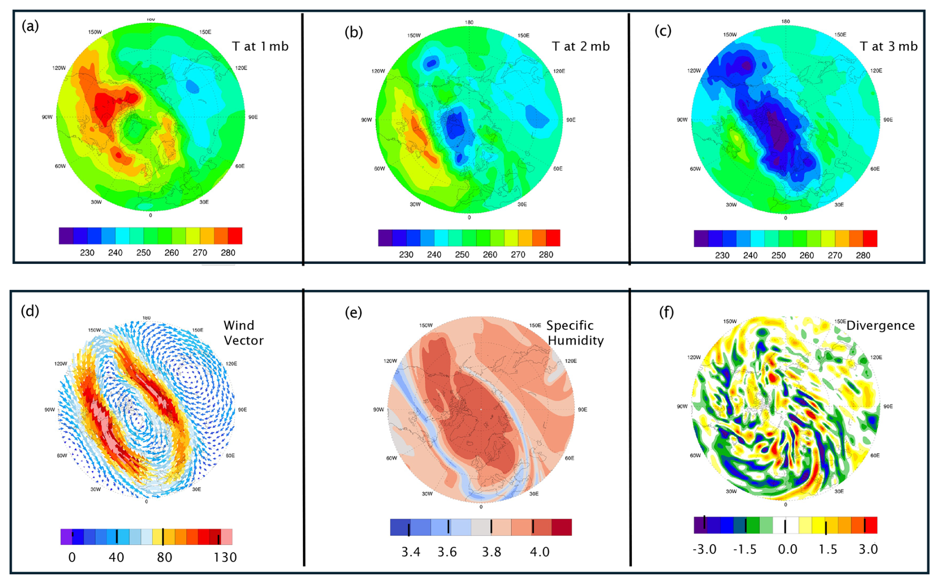
Figure 3 Distribution of the temperature on the 1, 2 and 3 mb surfaces (upper row) and the wind vector (ms⁻¹), specific humidity (10⁻⁶ kg kg⁻¹) and divergence (10⁻⁵ s⁻¹) on the 2 mb surface (lower row) for the same time instant as Fig. 2 (Based upon the ERA-Interim Reanalysis.).

Figure 3 displays, for the same time instant as Fig. 2, the distributions of the temperature on the 1, 2 and 3 mb pressure surfaces (Fig. 3a–c), and the wind vector field (Fig. 3d), the specific humidity (Fig. 3e) and the divergence patterns (Fig. 3f) on the 2 mb surface. The temperature fields are comparatively smooth and indicate that the SPV's cold pool weakened above 2 mb. In general, they do not exhibit the finer-scale features of the corresponding PV and relative vorticity patterns, whereas the stratification/static stability (not shown) at the PV maxima as determined in terms of the potential temperature difference between the different pressure levels, is typically twice that of the adjacent areas. These two contrasting facets of the thermal structure are in harmony with the forementioned vertical coherence of the PV features that attain a maximum amplitude at stratopause levels.

The wind vector field (Fig. 3d) pinpoints the location of the jet, and it is evident that the jet's overall strength suffices to substantially conceal the wind signature of the individual SSS features. In passing we note that a convenient ad hoc measure of the SPV's core is the domain located poleward of zero relative vorticity (see Figs. 2 and 3d). In the ERA-Interim Reanalysis the specific humidity is inert and merely advected with the in-situ winds and hence is akin to a flow tracer. Its distribution (Fig. 3e) is suggestive of a well-mixed SPV core that is substantially encircled by an elongated streamer of low humidity values advected on a different potential temperature surface.

The amplitude of the divergence field (Fig. 3f) is typically less than a quarter of the corresponding relative vorticity (and the corresponding absolute vorticity) values of the SSS features, and its spatial pattern is more reminiscent of buoyancy/gravity waves. This suggests that the dynamics of the sub-planetary scale features at stratopause elevations has a strong quasi-barotropic component. This lends a measure of credence to our later adoption of a barotropic theoretical model.

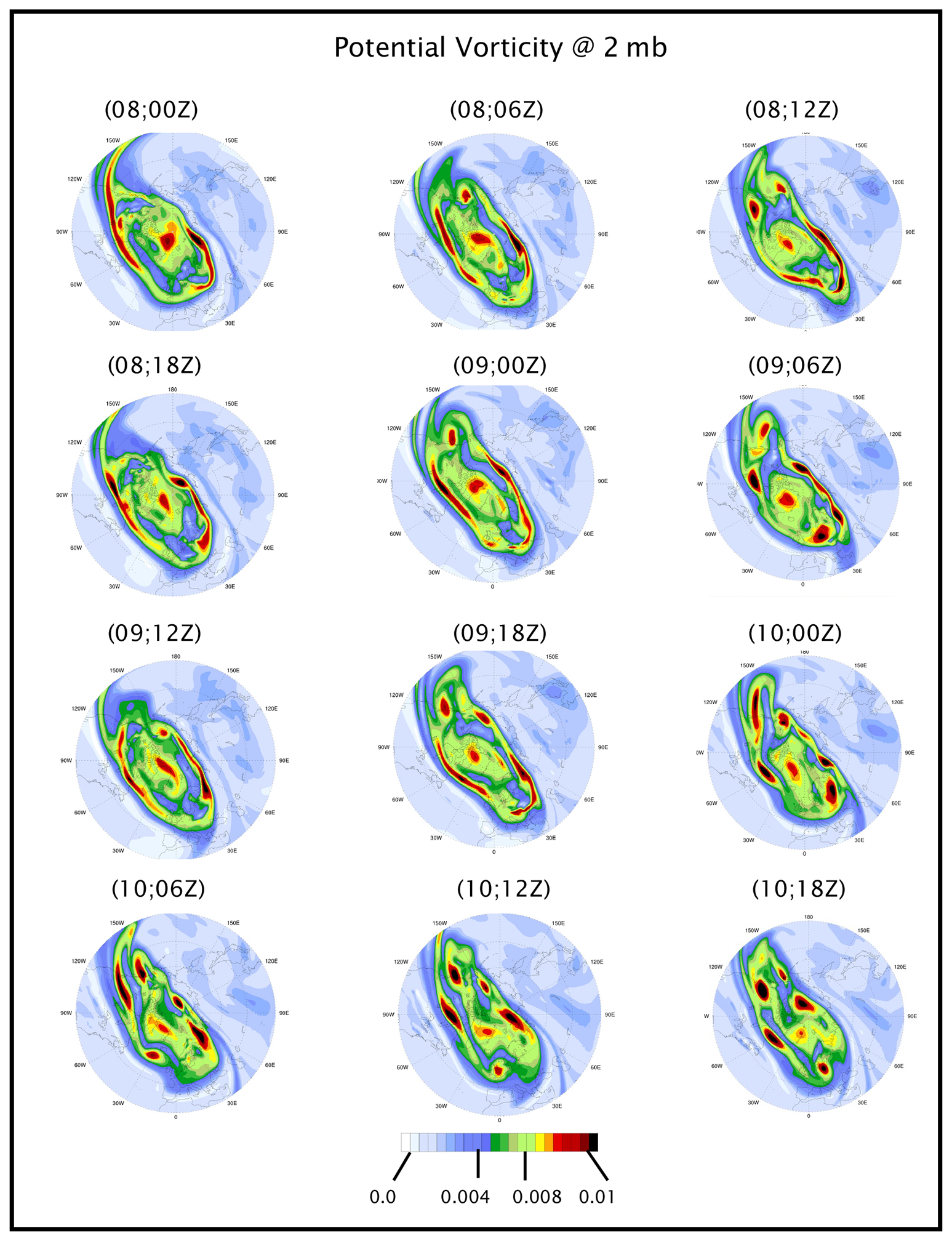
Figure 4 Evolution of the PV (K m² kg⁻¹ s⁻¹) on the 2 hPa pressure surface at 6 hourly intervals from 00:00Z on the 8 January to 18:00Z on the 10 January.

The prior development of the PV pattern depicted in Fig. 2c is shown in Fig. 4. It displays a 6 hourly time-sequence of the corresponding patterns to 00:00Z 11 January. The fragmented annulus is seen to evolve with time and the individual embedded SSS features are readily identified exhibiting a measure of temporal coherence as they are both advected by, and serve to modify, the in-situ flow. Note that the panels in Fig. 4 display the PV pattern on the 2 hPa surface. This renders ready comparison with the patterns of other variables shown on the 2 hPa surface in Figs. 2 and 3. In the subsequent case studies the evolution of the PV pattern is shown on the dynamically more instructive isentropic surfaces.

2.4 Features of a nascent SPV

The Austral winter stratosphere is less subject to PRW forcing from below, and here we examine the SPV during late Spring/early Southern Hemisphere winter of 2018. On the 10 mb pressure surface, the nascent SPV in April has a weak pole-centred PV anomaly, and by mid-May the jet's mean zonal flow had increased to ∼60 m s⁻¹ (Fig. 5a). In late April through early May there is evidence of a weak eastward propagating m=1 wave (Fig. 5b) but it disappeared by mid-month. The accompanying polar temperature had decreased by mid-May to ∼200 K with a pole-to-30° S temperature difference of some 25 K (not shown).

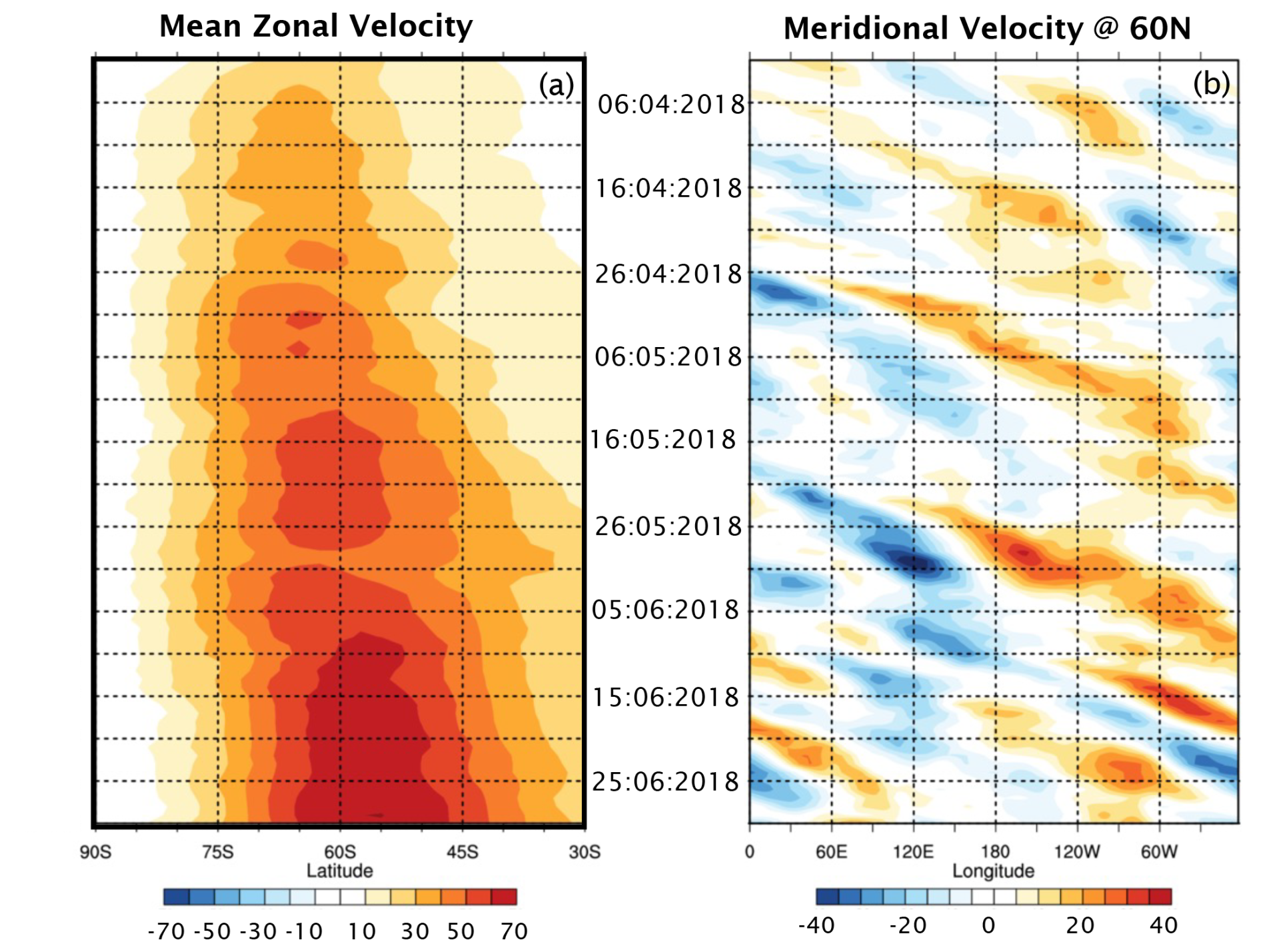
Figure 5 Counterpart of Fig. 1 but for April–June 2018 in the Southern Hemisphere at 10 mb. The zonal velocity now pertains to the latitude range 30–90° S, and the meridional velocity field is for 60° S.

Above, at stratopause levels, the localized region of high PV at the SPV's core began to break apart in early May and thereafter had a fragmented structure. Here the focus is on the synoptic-scale features in mid-month. Fig. 6 shows the PV, relative vorticity, divergence, potential temperature, ozone mass mixing ratio, and wind vector patterns on the 1 mb pressure surface at 00:00Z on 19 May. A train of isolated PV centres circumscribes the Hemisphere near 60° S with another PV feature in the neighbourhood of the pole (Fig. 6a). The train is also readily identifiable in the relative vorticity pattern (Fig. 6b) with, as in the previous case, peak amplitudes greater than 1.2×10⁻⁴ s⁻¹ – a value an order of magnitude stronger than that of the less organized divergence/gravity-wave field (Fig. 6c). The depth of the train itself extends downward at least over a scale depth with similar co-located patterns present on the 2 and 3 mb surfaces.

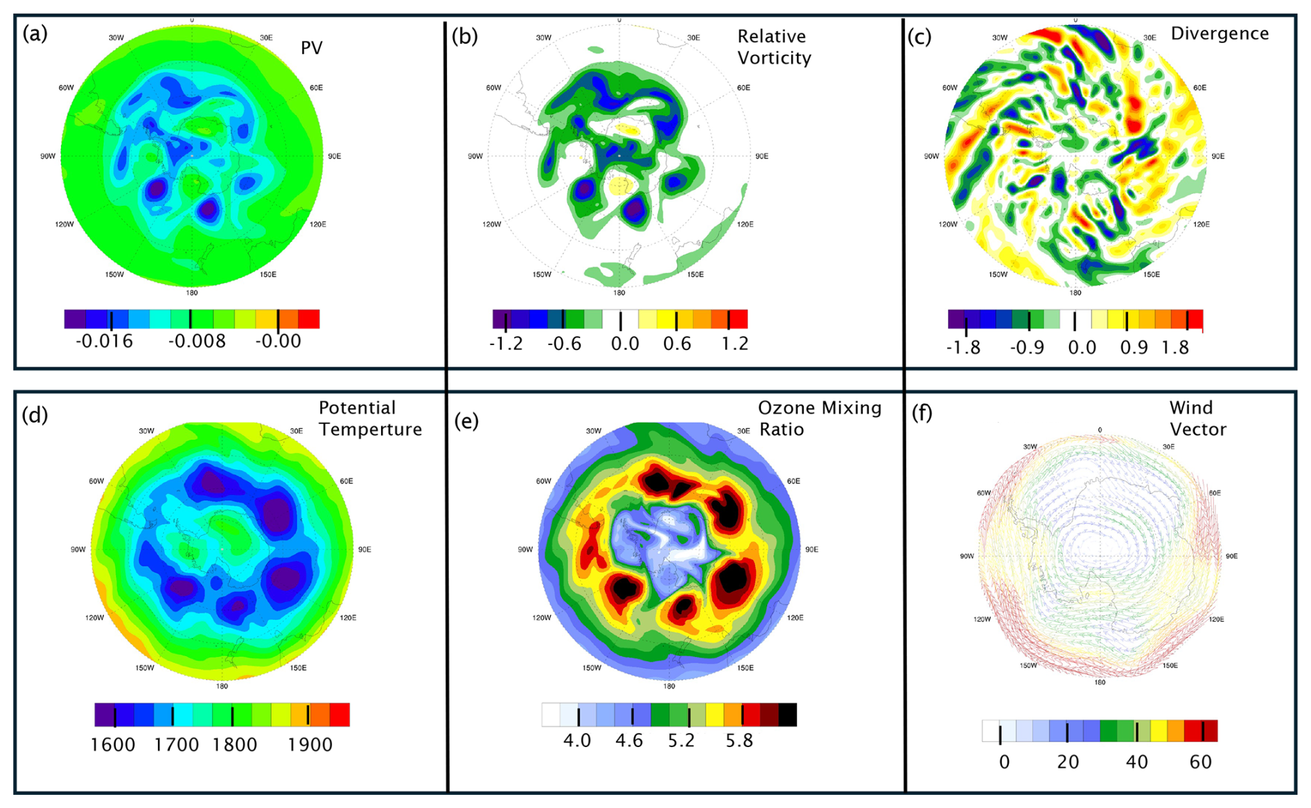
Figure 6 Depiction of the PV (K m² kg⁻¹ s⁻¹), relative vorticity (10⁻⁴ s⁻¹), divergence (10⁻⁵ s⁻¹), potential temperature (K), ozone mass mixing ratio (10⁻⁶ kg kg⁻¹), and wind vector (ms⁻¹) patterns on the 1 mb pressure surface at 00:00Z on 19 May. The panels are polar stereographic projections poleward from 30° S, except for panel (f) which is only poleward from 60S.

The potential temperature (θ) field (Fig. 6d) shows that at the 1 mb level the train is accompanied by a co-located zonal band of low potential temperature (∼1650 K). One possible inference is that the forementioned polar PV feature is located on a higher isentropic surface (around θ–1800 K). Saliently, the contemporaneous distribution of the ozone mass mixing ratio (Fig. 6e), shows not only a rich pattern of lower O₃ values within the SPV's core, but also a string of high values coincident with the vortex train itself. The latter is consistent with the presence of raised isentropic surfaces beneath the features of enhanced PV. Finally, the wind vector pattern (Fig. 6f) is consistent with the existence of strong shear on the poleward side of the jet and the presence of troughs linked to the stronger vortices of the train.

Figure 7 gives an indication of the prior development and movement of the isolated SSS features in the period from the 15–20 May. It depicts at daily interval the PV pattern on the 1700 isentropic surface and shows that the features advect eastward with, and are deformed by, the in-situ flow. To a measure they retain their amplitude pointing to their predominantly adiabatic character. Their temporal development is reminiscent of the downstream growth of a vortex train forming on a barotropically unstable shear layer rather than a synchronous development of vortices on such a layer. A noteworthy feature is that Figs. 6a and 7e display a close correspondence of both the individual features and the rim-like structure on the pressure and isentropic surfaces.

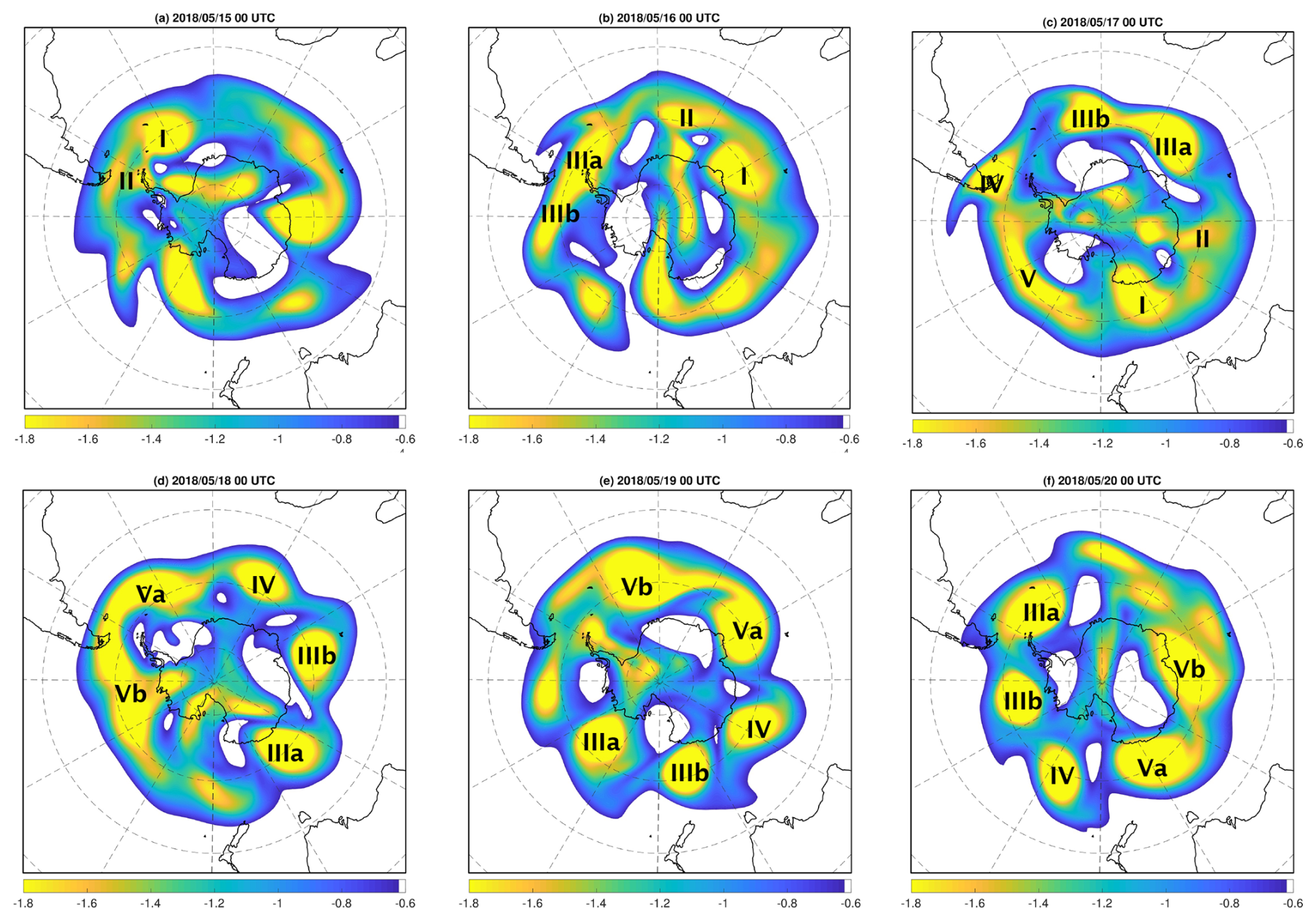
Figure 7 Evolution of the PV pattern at stratopause levels on the 1700 K isentropic surface at daily intervals from 00:00Z on the 15 May–20 May 2018. The labels I, II etc. attached to the PV maxima indicate the successive locations of the individual features (Units: km² kg⁻¹ s${}^{-\mathrm{1}}\times {\mathrm{10}}^{\mathrm{2}}$).

2.5 Features related to an SSW

A notable Sudden Stratospheric Warming occurred in February 2018, and it has subsequently been the subject of considerable scrutiny. This includes consideration of the event's development (Butler et al., 2020), the contribution of GWD (Watanabe et al., 2022), its dynamics and predictability (Rao et al., 2018; Karpechko et al., 2018; Knight et al., 2020; Erner et al., 2020), the accompanying middle atmosphere chemical signature (Perot and Orsolini, 2021), its difference to the 2019 SSW (Butler et al., 2020), its impact upon the mesosphere (Wang et al., 2019), and role of surface conditions in its occurrence (Lu et al., 2020). Here we briefly consider the planetary-scale and annular features of this SSW.

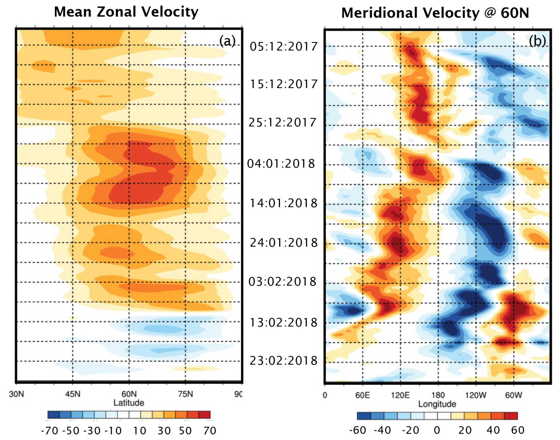
Figure 8 is the counterpart of Fig. 1 but for the 2017–2018 Boreal Winter. It shows that at 10 mb the zonal mean velocity (Fig. 8a) strengthened during the last week of December, attained a maximum of ∼60 m s⁻¹ in early January, deaccelerated to ∼30 m s⁻¹ in the period from the 14–19 January, and subsequently oscillated about this value before finally reversing around the 11 February. The time-longitude section for the meridional velocity at 60° N (Fig. 8b) indicates the presence of significant planetary scale wave patterns. The m=1 wave present in December was supplemented by an m=2 signal in January and subsequently supplanted by the latter ahead of the SSW event. Polar temperature tended to decrease to the 10 January, increased by ∼15 K by the 19 January, and oscillated thereafter until the onset of the SSW (not shown).

Figure 8 As for Fig. 1 but for the Winter of 2017–2018.

Above, at stratopause levels, the presence of the forementioned planetary scale waves were evidenced first by an off-pole PV pattern in December, and a dumb-bell off-pole pattern in January that distorted in the run up to the SSW. Figure 9 shows the patterns of the PV (left column), relative vorticity (centre column) and temperature (right column) on the 1 mb (upper row), 2 mb (middle row) and 10 mb (lower row) surfaces at a time (00:00Z 12 February) shortly after the SPV had satisfied the standard empirical criteria for an SSW. A distinctive and strong split of the SPV's PV distribution is evident at all three levels. The PV patterns on the upper two levels are similar (as are the relative vorticity patterns), and the range of the temperature fields are also similar. The near-pole temperatures are relatively low (high) at the upper levels (lower level). Together these flow and thermal patterns attest to the vertical coherency of an anomalous PV structure that is “effectively” centred near or below the 2 mb surface.

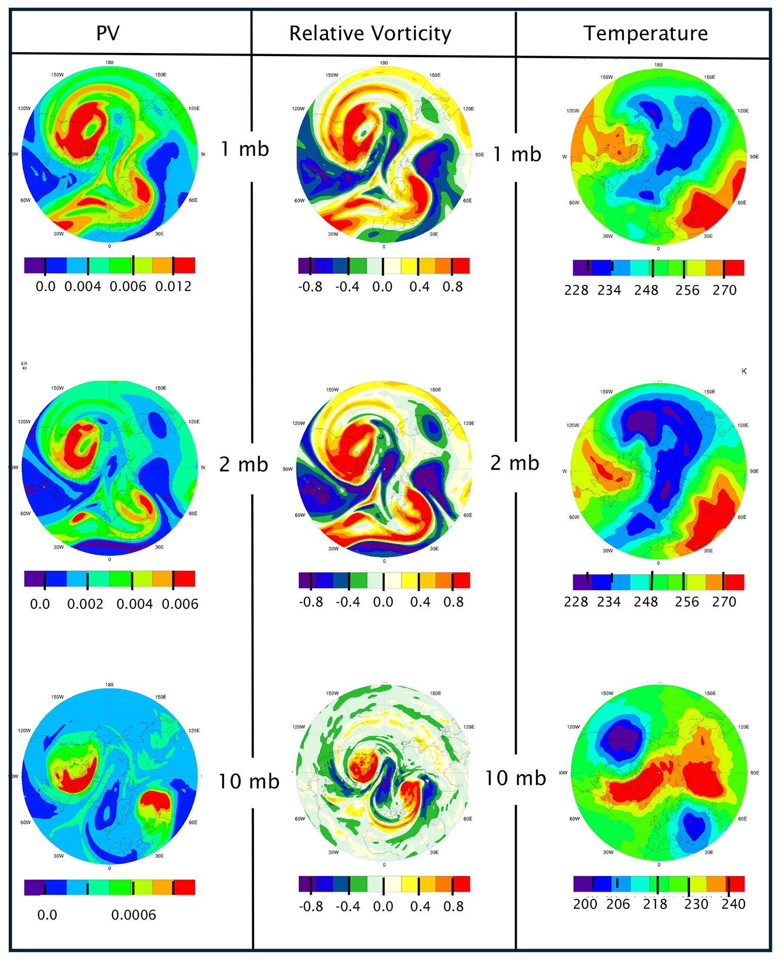
Figure 9 Distribution of the PV (K m² kg⁻¹ s⁻¹) in the left column, relative vorticity (10⁻⁴ s⁻¹) in the centre column, and potential temperature in the right column on the 1, 2, and 10 mb pressure surfaces at 00:00Z 12 February (shortly after the SSW).

Figure 10 portrays the development of the PV pattern at upper and mid-stratospheric levels at 48 h intervals immediately ahead of the satisfaction of the SSW criterion. The upper row depicts the patterns on the 1500 K isentropic surface at 00:00Z on the 6, 8 and 10 February, and the lower row shows the corresponding patterns on the 850 K isentropic surface.

Figure 10 The upper row displays the PV patterns in the upper stratosphere on the 1500 K isentropic surface at 00:00Z for the 6, 8 and 10 February, and the lower row shows the corresponding patterns but on the 850 K surface. The labels A, B, C etc. attached to individual PV maxima identify the successive location of the individual features (Units: km² kg⁻¹ s${}^{-\mathrm{1}}\times {\mathrm{10}}^{\mathrm{6}}$).

On the higher surface an annular-like structure is evident on the 6 February in the form of an off-pole elliptical structure with embedded sub-planetary scale features. It begins to fragment between the 6 and 8 February, and by the 10 February notable PV maxima have formed over Canada and western Europe. On the lower theta surface, the initially compact elliptic PV structure (Fig. 10d), first distends (Fig. 10e) and then splits (Fig. 10f). An inference is that the vortex is disrupted earlier and more severely on a higher θ surface.

The corresponding thermal patterns (not shown) on the upper (2 mb) and lower (10 mb) levels possess a dipole structure of opposite polarity that reverses with time. From the 10–12 February the near polar-temperature changes at the 1, 2, and 10 mb levels are respectively −18, −32, and +16 K.

2.6 Assessment of the Results

The foregoing case studies are for three fundamentally different flow settings and are focused on the finer-scaled flow features contiguous to, or related to, the structure of the Stratospheric Polar Vortex's periphery at stratopause levels. In particular, they sought to capture the essence of their scale, structure, temporal evolution, and dynamics.

The results show the features to be present in all three flow settings as synoptic-scale PV extrema located principally on the vortex's periphery in both hemispheres with associated relative vorticity values of ∼10⁻⁴ s⁻¹ and extending typically at least a scale-depth below the stratopause. The temperature and horizontal divergence patterns do not have a comparable localized signal on pressure surfaces located at stratopause levels. Together these features are consistent with deep isolated PV features centred near the stratopause with associated strong static stability at their core and weak quasi-horizontal temperature gradients at their centre. Also taken together the amplitude and synoptic-scale of the vorticity centres and the significantly weaker amplitude of their divergence suggests that the contribution of the horizontal divergence term to the development of the vertical component of vorticity is weak. This is not inconsistent with the adoption of an idealized barotropic model in the study's theoretical component (Sect. 3).

Again, the distinctive pattern of the ozone mixing ratio is consistent with the existence and dynamical signature of the isolated PV features whilst the space-time development of the PV pattern itself on key isentropic surfaces sheds light on their translation, development and conservation. In effect these transient sub-planetary and synoptic scale, predominantly monopole, positive PV (and relative vorticity) anomalies translate with and distort the ambient SPV's flow. These observationally based characterization of the PV features underlines the desirability of establishing the climatology of the features. In this context we note for example that at the 2 mb level on every 15 January of the 41 year ERA-Interim data set, SSS features and/or an annular-like structure were present on 24 d, the PV vortex was severely disrupted on another 16 d (of which 11 were related to major or minor SSW events at 10 hPa), and on one day there was a single pole-centred PV vortex.

The presence of the features can in principle contribute to the distribution of chemical constituents within the core. Their existence near the core's periphery suggests that they can modify the perceived width of the SPV, potentially help mix air both within the core and across its periphery, and serve to diffuse the jet (Bowman and Chen, 1994; Ishioka and Yoden, 1995; Mitzu and Yoden, 2001). The latter surmise points to their possible role, in addition to GWD, in reducing the jet strength at and above the stratopause. Again, the predominantly monopole structure of the features is consistent with their predilection to evolve from a banded structure of enhanced PV near the SPV's periphery and is strongly reminiscent of the growth to finite amplitude of perturbations of a barotropically unstable flow. Also, the break-up of the stratopause-level annular band of enhanced PV during a Sudden Stratospheric Warming event opens the possibility that the band might participate in, and contribute to, the initial development of such an event.

3 Theoretical Model Studies

Our objective here is to explore the character of perturbations that can evolve on an annular-like flow structure akin to that of a deep, axisymmetric and undisturbed SPV. To this end we parsimoniously adopt an idealized theoretical model capable of representing fundamental features of such a setting including the occurrence of barotropic instability. The model constitutes non-divergent barotropic flow on a polar β-plane. It can sustain a basic state of a cylindrical (possibly unstable) jet, and it incorporates a suitable representation of the latitudinal variation of the Coriolis effect but excludes consideration of three-dimensional effects, and therefore best represents flows structures that are comparatively deep. These restrictions, together with the model's simple configuration, imply that our results will constitute a potentially insightful qualitative guide rather than providing quantitative definitive statements.

3.1 Model Configuration and Methods of Analysis

On a polar β-plane the earth's vorticity is given by

$$f=\mathrm{2}\mathrm{\Omega }\left[\mathrm{1}-\mathrm{1}/\mathrm{2}{\left({\displaystyle \frac{r^{*}}{R}}\right)}^{\mathrm{2}}\right],$$

where r^* denotes radial distance on the plane and R refers to the Earth's radius. Then the model's governing equation takes the form

$$\begin{array}{}\text{(1)}& D\left(Z^{*}\right)/D{t}^{*}=\mathrm{0}\end{array}$$

where $D/D{t}^{*}$ denotes the material derivative for two-dimensional flow, and Z^* is the “system-relative” absolute vorticity

$$Z^{*}=z^{*}-\mathrm{2}\mathrm{\Omega }\left[\mathrm{1}/\mathrm{2}{\left(r^{*}/R\right)}^{\mathrm{2}}\right].$$

Here ζ^* denotes the relative vorticity and is such that ${\mathit{\zeta }}^{\ast }={\mathrm{\nabla }}^{\mathrm{2}}{\mathit{\psi }}^{\ast }$ with ψ^* denoting the stream function. In the following the dimensional starred variables are replaced by non-dimensional unstarred variables: $r=r^{*}/R$, $Z=Z^{*}/\left(\mathrm{2}\mathrm{\Omega }\right)$, $\mathit{\zeta }={\mathit{\zeta }}^{\ast }/\left(\mathrm{2}\mathrm{\Omega }\right)$, and an azimuthal velocity $V=V^{*}/\left(\mathrm{2}\mathrm{\Omega }R\right)$.

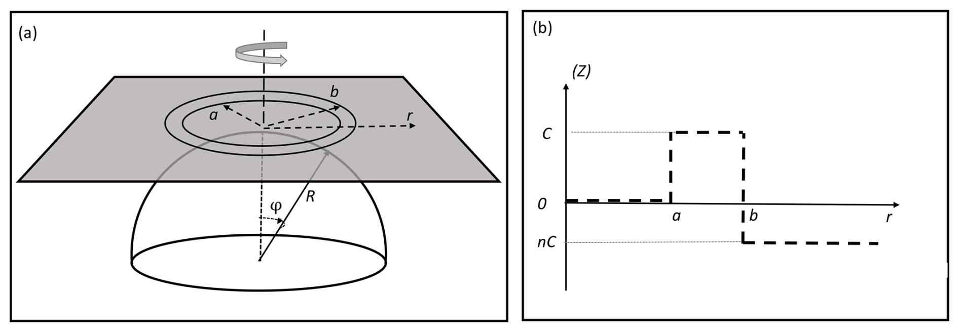
Figure 11 Panel (a) is a schematic of the polar β-plane and the geometry for the initial distribution of the vorticity. Panel (b) shows the radial distribution of three concentric zones of uniform Z (displayed as heavy dashed lines) such that there is annular band of enhanced Z located between $(a<r<b)$.

To facilitate the derivation of analytical results we let the “system relative” absolute vorticity of the undisturbed circumpolar vortex comprise three concentric zones (see Fig. 11) of respective uniform absolute vorticity (Z_I, Z_II, Z_III), given by

$$\begin{array}{}\text{(2a)}& {\displaystyle }{Z}_{\mathrm{I}}=\mathrm{0},\mathrm{for}r<a,\text{(2b)}& {\displaystyle }{Z}_{\mathrm{II}}=C,\mathrm{for}a\le r\le b,\text{(2c)}& {\displaystyle }{Z}_{\mathrm{III}}=nC,\mathrm{for}r>b.\end{array}$$

This represents a relatively quiescent innermost core (r<a), an annular region ($a\le r\le b$) yielding an absolute vorticity maximum, and an outer domain (r>b) of weaker vorticity (i.e. n<0).

The accompanying axisymmetric basic flow (V) takes the form

$$\begin{array}{}\text{(3a)}& {\displaystyle }{V}_{\mathrm{I}}=\left(\mathrm{1}/\mathrm{8}\right)r^{\mathrm{3}},\mathrm{for}r<a,\text{(3b)}& {\displaystyle }{V}_{\mathrm{II}}=(\mathrm{1}/\mathrm{2})\mathrm{Cr}\left[\mathrm{1}-{\left(a/r\right)}^{\mathrm{2}}\right]+\left(\mathrm{1}/\mathrm{8}\right)r^{\mathrm{3}}\mathrm{for}a\le r\le b,\text{(3c)}& {\displaystyle }\begin{array}{rl}& V_{\mathrm{III}}=(\mathrm{1}/\mathrm{2})\mathrm{Cr}\left[n+{\left(b/r\right)}^{\mathrm{2}}(\mathit{\epsilon }-n)\right]+\left(\mathrm{1}/\mathrm{8}\right)r^{\mathrm{3}}\\ & \mathrm{for}r>b.\end{array}\end{array}$$

It is also pertinent to note that,

$$\begin{array}{}\text{(4)}& {\displaystyle }\left({\displaystyle \frac{V_a}{a}}\right)=\left(\mathrm{1}/\mathrm{8}\right)a^{\mathrm{2}},\text{(5)}& {\displaystyle }\left({\displaystyle \frac{V_b}{b}}\right)=(\mathrm{1}/\mathrm{2})\left[C\mathit{\epsilon }+\left(\mathrm{1}/\mathrm{4}\right)b^{\mathrm{2}}\right],\end{array}$$

where ($V_{\mathrm{a}}/a$) and ($V_{\mathrm{b}}/b$) denote respectively the angular velocity at r=a and b.

Here $\mathit{\epsilon }=[\mathrm{1}-{\left(a/b\right)}^{\mathrm{2}}]$ is a measure of the width of the annular region relative to its radial location, and the $(\mathrm{1}/\mathrm{8})r^{\mathrm{3}}$ term in Eq. (3a)–(3c) is attributable to the β-effect. In effect the parameters ($a,b,C,n$) determine the basic state of the vortex core, with typically $C\le \mathrm{2},b\sim \mathrm{1}/\mathrm{2}$, and a and b such thatϵ is capable of spanning across its permissible [0,1] range.

The parameter (nC) determines the relative vorticity (ζ) distribution in the exterior (i.e. ${\mathit{\zeta }}_{\mathrm{III}}=nC+\mathrm{1}/\mathrm{2}{r}^{\mathrm{2}}$). Its value is bounded by the requirements that the absolute vorticity in the far-field be less than in the polar region (nC<0), and the basic state flow should be inertially stable (nC>−1). A more stringent condition is the requirements that at a radial distance, say r=r_c, the velocity is significantly reduced and ζ approaches zero (i.e. $nC\sim -\mathrm{1}/\mathrm{2}{r}_c^{\mathrm{2}}$). For such a reduction to occur by say ∼30° N then typically $\mathrm{0.7}>r_c>\mathrm{1.2}$.

Figure 12 shows illustrative examples of the basic state flow profiles (V) representable by Eq. (3). For the r≤b domain, the jet profiles correspond to maxima of 90 m s⁻¹ and 135 m s⁻¹ located at $b=\mathrm{1}/\mathrm{2}$ (≈60° N), for wide (ϵ = 0.91), intermediate (ϵ = 0.75) and narrow (ϵ = 0.36) annuli. Note that, for C in the range ($\mathrm{1}/\mathrm{2}$–2) and ϵ in the range ($\mathrm{3}/\mathrm{4}\mathrm{-}\mathrm{1}$), then $v_b\approx \mathrm{1}/\mathrm{4}\left(C\mathit{ϵ}\right)$, and the velocity profiles shown in the outer domain (r>b) span those for realistic values of r_c. In essence Fig. 12 shows that the parameter settings permit a range of appropriate velocity profiles.

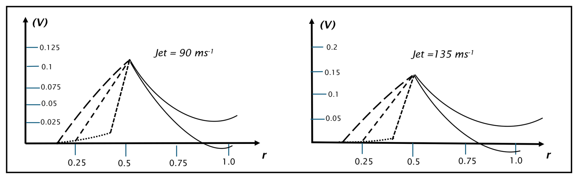
Figure 12 A sample of the model's possible basic state velocity (V) profiles corresponding to a dimensional jet strength of 90 m s⁻¹ (left) and 135 m s⁻¹ (right) located at $b=\mathrm{1}/\mathrm{2}$ (≈60° N). In each panel the three curves for r<b, depicted with long, intermediate and short dashes, refer respectively to wide (ϵ = 0.91), intermediate (ϵ = 0.75), and narrow (ϵ = 0.36) annuli, and the dotted line is the velocity profile, where applicable, in the r<a sector. The two full curves beyond r=b encompass the physically constrained band (i.e. $\mathrm{0.7}>r_c>\mathrm{1.2}$) of velocity profiles (For the specific values of C see the legend to Fig. 13).

Results are derived for the linear and non-linear response of perturbations of stipulated basic states. The linear component includes a normal mode analysis that establishes the growth rate and azimuthal wavenumber (m) of unstable modes, and an analysis of the response to a specific form of non-normal mode initial perturbation. The non-linear response is simulated using a contour-dynamics technique (Dritschel, 1989a) with adjustments of the standard contour advection technique to (a) account for the specification of the absolute as opposed to the relative vorticity and (b) circumvent the standard contour advection stipulation of non-zero absolute vorticity in the outermost domain. The forward integration is conducted using a 4th order Runge-Kutta scheme and, depending upon the purpose of the simulation, the initial state is perturbed by adding either weak amplitude random noise to the location of the interfaces or a finite amplitude displacement to the location of the interface at r=b.

3.2 Normal Mode Analysis

3.2.1 Derivation of the Instability Criterion

Small amplitude perturbations of the governing equation (Eq. 1) satisfy the linear equation,

$$\begin{array}{}\text{(6)}& \mathit{\{}\partial /\partial t+(V/r)\partial /\partial \mathit{\theta }\mathit{\}}{q}^{\prime }+u^{\prime }\partial /\partial r\left(Z\right)=\mathrm{0}\end{array}$$

Here (q^′, u^′) refer to the perturbation vorticity and radial velocity with $q^{\prime }={\mathrm{\nabla }}^{\mathrm{2}}{\mathit{\psi }}^{\prime }$. Likewise, (Z,V) are, as indicated earlier, the basic state absolute vorticity and azimuthal velocity (Eqs. 2 and 3).

Adopting a “PV Perspective” for the perturbations (Davies and Bishop, 1994) solutions of Eq. (6) are sought for stream-function perturbations (ψ^′) of the form

$${\mathit{\psi }}^{\prime }={\mathit{\psi }}_{\mathrm{a}}^{\prime }+{\mathit{\psi }}_{\mathrm{b}}^{\prime }$$

where the two components represent wave perturbations propagating respectively on the vorticity discontinuities at the domain interfaces located at r=a and b. The associated stream functions are

$${\mathit{\psi }}_{(a,b)}^{\prime }=F_{(a,b)}\left(r\right)\sin (m\mathit{\theta }-\mathit{\omega }t)$$

and for basic states of the form given by Eq. (3), F has a r^m and r^−m dependency respectively within and exterior to the pertinent interface. On applying appropriate conditions at r=0, as r−>∞, and at the interfaces, the wave amplitudes at the two interfaces, $F_{(a,b)}=$ (A, B), are linked by the relationships,

$$\begin{array}{}\text{(7a)}& {\displaystyle }\left({\displaystyle \frac{\mathit{\omega }}{m}}\right)A=(V_a/a)A+(\mathrm{1}/\mathrm{2})(C/m)[A+{\left(\mathrm{1}-\mathit{\epsilon }\right)}^{m/\mathrm{2}}B],\text{(7b)}& {\displaystyle }\begin{array}{rl}\left({\displaystyle \frac{\mathit{\omega }}{m}}\right)B& =\left({\displaystyle \frac{V_b}{b}}\right)B-(\mathrm{1}/\mathrm{2})\left({\displaystyle \frac{C}{m}}\right)(\mathrm{1}-n)\\ & [B+{\left(\mathrm{1}-\mathit{\epsilon }\right)}^{m/\mathrm{2}}A].\end{array}\end{array}$$

The three-terms on the right-hand side in each of Eq. (7a) and (7b) correspond respectively to: translation with the ambient angular velocity (Eq. 3d, e); a “Rossby-wave type” contribution of the in-situ wave; and a far-field “Rossby-wave type” contribution due to the influence of a wave at one interface acting upon that at the other interface. In the absence of the latter far-field contributions, equivalence of the phase velocities would require – see Eqs. (4) and (5)

$$\begin{array}{}\text{(8a)}& \mathcal{D}=\mathrm{0}\end{array}$$

where

$$\begin{array}{}\text{(8b)}& \mathcal{D}=\left[m\mathit{\epsilon }\right(\mathrm{1}+\mathit{\mu })-(\mathrm{2}-n\left)\right]\end{array}$$

with $\mathit{\mu }=b^{\mathrm{2}}/\left(\mathrm{4}C\right)$.

We return to consider the import of Eq. (8a) later but proceed here to note that together Eq. (7a) and (7b) yield the linear system's wave-dispersion relationship. After some manipulation the instability criterion can be written as

$$\begin{array}{}\text{(9a)}& \mathrm{\Delta }>\mathrm{0},\end{array}$$

with

$$\begin{array}{}\text{(9b)}& \mathrm{\Delta }=\left[-{\mathcal{D}}^{\mathrm{2}}+\mathrm{4}\left(\mathrm{1}-n\right){\left(\mathrm{1}-\mathit{\epsilon }\right)}^m\right],\end{array}$$

and for unstable waves, the growth rate (σ) and angular phase speed (v) are given by,

$$\begin{array}{}\text{(9c)}& {\displaystyle }\mathit{\sigma }=(\mathrm{1}/\mathrm{4})C\sqrt{\left(\mathrm{\Delta }\right)},\text{(9d)}& {\displaystyle }v=(\mathrm{1}/\mathrm{2})\left[(V_a/a+V_b/b)+\left(nC\right)/m\right],\end{array}$$

In line with the necessary criteria for barotropic instability the annular region needs to be a maximum of absolute vorticity (see Eq. 9b), i.e. (1−n)>0.

3.2.2 Sample Growth Rate Curves

A sample of the dependency of the instability upon the configuration of the basic state is illustrated in Fig. 13. It shows the growth rate (σ) as a function of the wavenumber (m) for settings corresponding to those referred to earlier (see Figs. 12 and 13). In terms of conventional flow parameters, the growth rate is seen to increase markedly with jet strength, decrease strongly as the sharpness of the jet decreases on its poleward side (i.e. width of the annulus increases), and is less sensitive to the velocity profile in the surf zone (as determined by the value of r_c). In effect for these settings the sensitivity to the jet skewness is primarily governed by the structure within the core. These results are in qualitative agreement with, and complement those of, earlier barotropic instability studies (see in particular Hartmann, 1983) but a significant difference (discussed further below) is the stability of the m=1or2 modes. The large growth rate of the sub-planetary modes is notable since a pragmatic lower bound for an unstable mode's growth rate would be that σ should exceed τ, where τ∼ (10 d)⁻¹ is the radiative decay timescale (Shine, 1987) of deep perturbations within the polar-night vortex in the upper stratosphere.

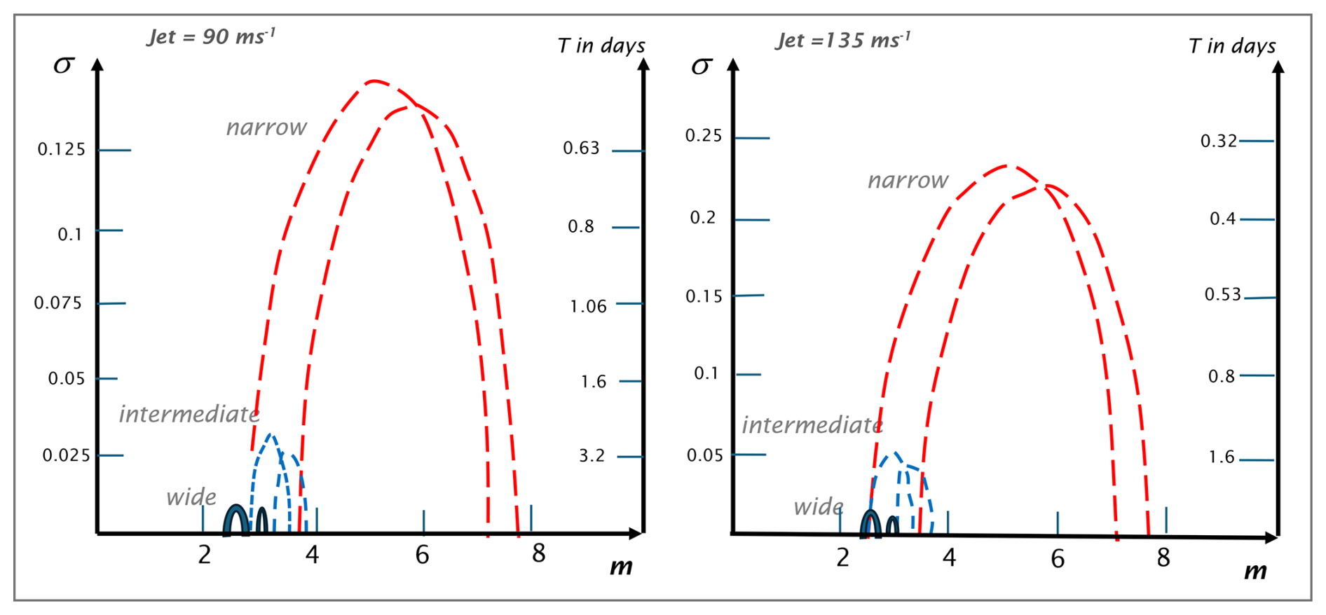
Figure 13 Growth rate (σ) displayed as a function of the wavenumber (m) for a jet of strength 90 m s⁻¹ (left) and 135 m s⁻¹ (right) located at $b=\mathrm{1}/\mathrm{2}$ (≈60° N). Note the differing scale of the ordinates. The dashed-red, dashed-blue and thick-black curves are for respectively: – narrow (ϵ = 0.36), intermediate (ϵ = 0.7); and wide (ϵ = 0.91) annular bands. For the 90 m s⁻¹ jet, the two curves for each of the three categories the [C,r_c] values are: – [0.91, (0.85–0.95); 0.44, (0.89–0.93); 0.36, (0.85–0.95)]. The corresponding values for the 135 m s⁻¹ jet are: – [1.44, (0.93–1.0); 0.69, (0.93–1.05); 0.57, (0.96–1.07)].

3.2.3 Dynamics of the Instability

Figure 13 provides a useful, but non-exhaustive, display of the unstable modes dependence upon the basic state configuration. Further numerous computations using Eq. (9c) would enable the sensitivity to the externally specified parameters (such as b) or combination of those parameters (such as μ) to be empirically inferred. Here in contrast we seek to deductively determine those sensitivities by pinpointing the dynamics underlying of the instability and thereby concomitantly establishing the wavenumber of the most unstable mode.

To this end we adopt the PV-based phenomenological interpretation (Lighthill, 1967; Hoskins et al., 1985) and mathematical formulation (Davies and Bishop, 1994) of barotropic and baroclinic instability. In this framework the present form of instability is viewed in terms of two counter propagating waves on the opposite-signed PV jumps at r=a and r=b that are held stationary relative to one another by the differing in-situ flow at their respective locations. In such a configuration the waves inter-dependency can promote mutual amplification and/or induce a modification of their azimuthal phase velocities.

The key to the instability dynamics comes from noting the implications of 𝒟= 0. First, phase locking of the two waves is achieved without an inter-wave contribution (see discussion leading to Eq. 8a) so that the two perturbations are in quadrature and their inter-wave influence is constrained to yield maximal growth. Second there is (see Eq. 9b) an azimuthal wave number (m₀) for which a wave perturbation is unstable with

$$\begin{array}{}\text{(10a)}& m_{\mathrm{0}}=(\mathrm{2}-n)/\left[\mathit{\epsilon }\right(\mathrm{1}+\mathit{\mu }\left)\right]\end{array}$$

In effect m₀ is the ratio of the sum of the two vorticity discontinuities to the difference in the angular velocities across the annular region. It can be reformulated as

$$\begin{array}{}\text{(10b)}& m_{\mathrm{0}}\mathit{\epsilon }=\mathrm{2}[\mathrm{1}+r_c^{\mathrm{2}}/(\mathrm{4}C\left)\right]/[\mathrm{1}+b^{\mathrm{2}}/(\mathrm{4}C\left)\right]\end{array}$$

It follows that, for specified values of the external parameters, satisfaction of Eq. (10a) and (10b) signifies the instability of the wavenumber m₀. The accompanying growth rate is given by Eq. (9c), so that

$$\begin{array}{}\text{(11a)}& \mathit{\sigma }=(\mathrm{1}/\mathrm{2})C{\left[\left(\mathrm{1}-n\right){\left(\mathrm{1}-\mathit{\epsilon }\right)}^m\right]}^{\mathrm{1}/\mathrm{2}},\end{array}$$

In conjunction with Eq. (10b) this can be recast in the form

$$\begin{array}{}\text{(11b)}& \mathit{\sigma }=(\mathrm{1}/\mathrm{2}){\left\{C\left[C+\mathrm{1}/\mathrm{2}\left(r_c^{\mathrm{2}}\right)\right]{\left(\mathrm{1}-{\displaystyle \frac{m_{\mathrm{0}}\mathit{\epsilon }}{m_{\mathrm{0}}}}\right)}^{m\mathrm{0}}\right\}}^{\mathrm{1}/\mathrm{2}}\end{array}$$

The third consequence of setting 𝒟=0 is that m₀ provides (for m₀>2) an excellent estimate of the wavenumber ($m=m^{*}$) of the most unstable mode. This follows from (a) deducing that,

$$\begin{array}{}\text{(12)}& (m^{*}/m_{\mathrm{0}})=\mathrm{1}+\mathit{\lambda }\mathit{\phi }\end{array}$$

where

$$\mathit{\lambda }=[\mathrm{1}+(\mathrm{1}/\mathrm{2}\left)r_c^{\mathrm{2}}\right]/[\mathrm{1}+r_c^{\mathrm{2}}/(\mathrm{4}C\left)\right][\mathrm{1}+b^{\mathrm{2}}/(\mathrm{4}C\left)\right]$$

and

$$\mathit{\phi }={\left(\mathrm{1}-\mathit{\epsilon }\right)}^{m^{*}}\ln (\mathrm{1}-\mathit{\epsilon })/\left(\mathit{\epsilon }\right)$$

and (b) noting from Fig. 14 that λ is less than or order 1 and $\mathit{\phi }\sim -\mathrm{0.1}$ for the range of pertinent basic state settings.

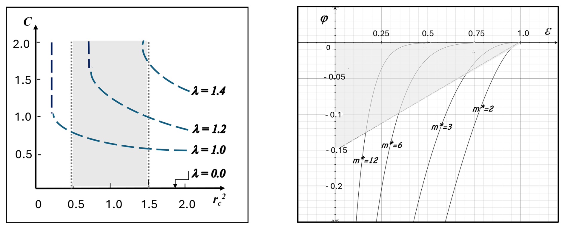
Figure 14 Left panel displays λ in the space of [(r_c)², C] for $b=\mathrm{1}/\mathrm{2}$ with the realistic range for r_c lightly shaded. Right panel shows φ as a function of ϵ for selected values of the wave number m^*, and the permissible domain is confined to the lightly shaded wedge-shaped region with (m^*ϵ) >2.0.

In summary the dynamics of the instability is encapsulated by the characteristics of the normal mode whose two interface waves are in quadrature (i.e. 𝒟= 0). It is unstable, its wavenumber (m₀) is an accurate estimate of that of the most unstable mode (m^*) for (m^*) >2, and it provides (via Eq. 10) a compact description of the sensitivity of m^* to the configuration of the basic state. Again, it demonstrates that the occurrence of unstable high wavenumbers (say, $m^{*}>\mathrm{8}$) requires narrower annular regions (small ϵ); unstable sub-planetary scale waves (say, $\mathrm{3}<m^{*}<\mathrm{8}$) exist for a wide range of external settings; and the graver modes ($m=\mathrm{1},\mathrm{2}$) are stable.

3.2.4 An Instability Ready Reckoner

The two panels of Fig. 15 are based upon Eq. (10) and together constitute an instability “Ready Reckoner”. For a stipulated specification of the external parameters, the procedure is as follows:

• (i)

  Fig. (15a) determines the value of (m₀ϵ) as a function of ${r_c}^{\mathrm{2}}$ and C (see Eq. 10b),

• (ii)

  an estimate m₀ of the most unstable wavenumber is then known given the specification of ϵ,

Furthermore, the factors influencing the growth rate and an estimate of that growth can be gleaned from inspection of Fig. 15b and in conjunction with Eq. (11b). It is noteworthy that the growth rate is highly dependent upon the value of C, favoured by higher values of ${r_c}^{\mathrm{2}}$, and is sensitive to the value of m₀ (see Fig. 15b).

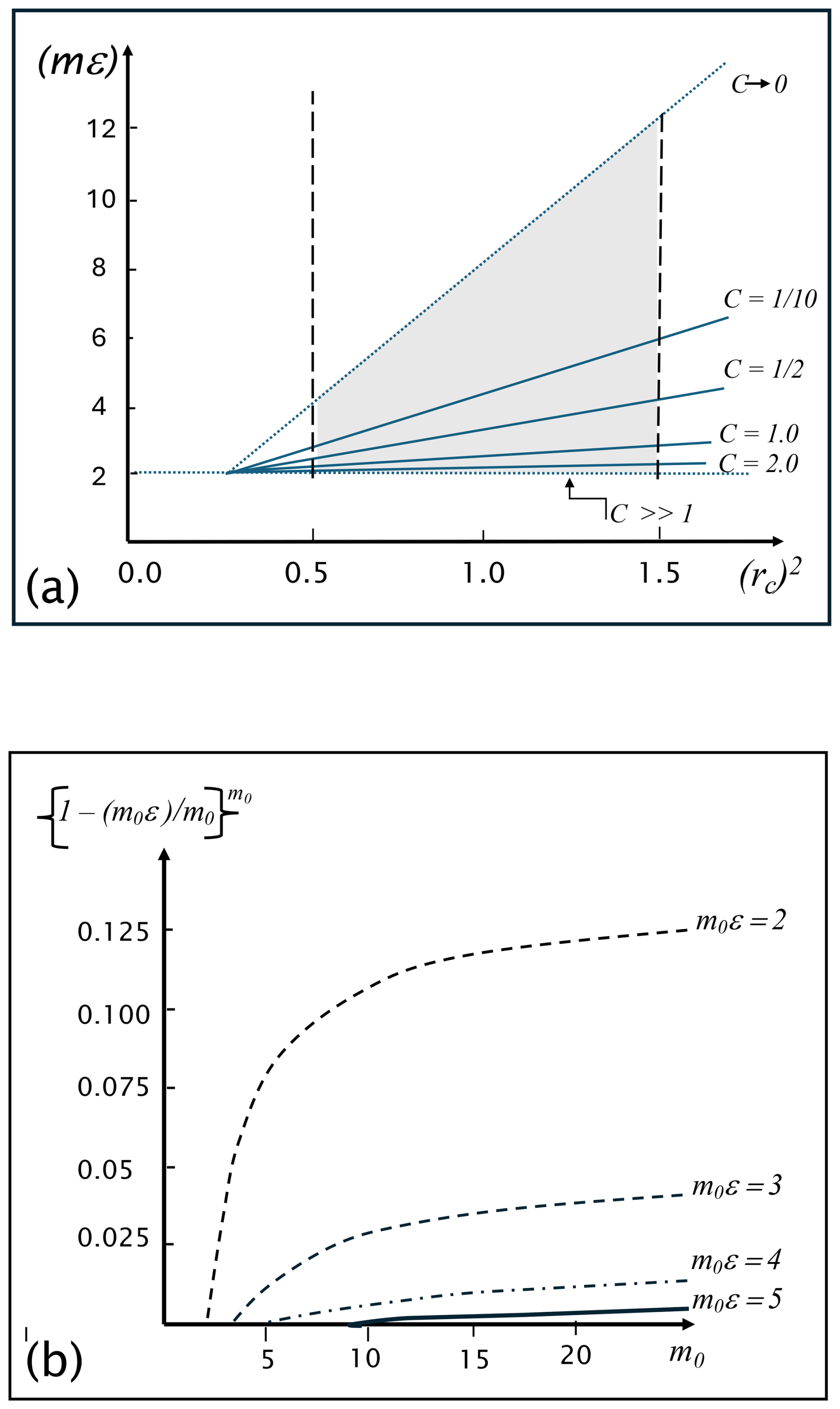
Figure 15 A sensitivity guide to the most unstable normal mode: Displayed in panel (a) is a plot of (m₀ϵ) as a function of (r_c)² for a range of C with $b=\mathrm{1}/\mathrm{2}$. Again the realistic range for r_c is the lightly shaded region. Panel (b) depicts the growth factor $\left(\mathrm{1}\mathrm{-}\right(m_{\mathrm{0}}\mathit{ϵ})/m_{\mathrm{0}}$)^m0 as a function of the wavenumber m₀.

In effect the Ready Reckoner is an indicator of the scale and growth rate of the most unstable modes over the realistic range of external parameters. Moreover, the results, in conformity with the observational cases studies of Sect. 2, indicate that sub-planetary and synoptic-scale features can evolve preferentially for a wide-range of realistic annular flow settings.

3.2.5 Stability of the m=1, 2 Modes

The character of the gravest modes ($m=\mathrm{1},\mathrm{2}$) are not adequately represented by Eqs. (10) and (11). However, they are of particular interest in connection with the occurrence of an SSW, and therefore merit special attention. For these two modes the instability criterion, sic. the parameter Δ (Eq. 9), equates to,

$$\begin{array}{rl}\mathrm{\Delta }& =-\mathit{\{}{\mathit{\epsilon }}^{\mathrm{2}}{\left(\mathrm{1}+\mathit{\mu }\right)}^{\mathrm{2}}-\mathrm{2}\mathit{\epsilon }[n+\mathit{\mu }(\mathrm{2}-n)]+n^{\mathrm{2}}\mathit{\}}\\ & \mathrm{for}m=\mathrm{1},\mathrm{and}\\ \mathrm{\Delta }& =-\mathit{\left\{}{\mathit{\epsilon }}^{\mathrm{2}}\right[\mathit{\mu }(\mathrm{2}+\mathit{\mu })+n]-\mathit{\epsilon }[n+\mathit{\mu }(\mathrm{2}-n)]+(n^{\mathrm{2}}/\mathrm{4}\left)\mathit{\right\}}\\ & \mathrm{for}m=\mathrm{2},\end{array}$$

with $\mathit{\mu }=\frac{b^{\mathrm{2}}}{\mathrm{4}C}$ and $n=-\mathrm{1}/\mathrm{2}{\left(r_c\right)}^{\mathrm{2}}/C$. For realistic values of μ and n, generally Δ<0, so that both modes are indeed stable. Notwithstanding Δ can be small ($\mathrm{0}>\mathrm{\Delta }>\mathrm{-}\mathrm{0.2}$) for m=2 across the entire range of ϵ values, and small for m=1 as ϵ–>0. (This will become a significant factor in the next sub-section when we consider a mechanism that runs counter to the non-growth of these normal modes.)

3.3 Initial-value Dependency

Consider a configuration of our model system that at the initial instant comprises a pre-existing small amplitude wave on the outer (r=b) interface but with no perturbation on the inner (r=a) interface. The analogue stratospheric setting would be the combination of: (a) the distortion of the outer interface by, say, a Rossby wave emanating from tropopause elevations and propagating upward preferentially along the waveguide formed by the sharp PV gradient on the polar vortex's outer edge; and (b) the inner interface being initially substantially undisturbed being protected by the reversed latitudinal PV gradient on an annular band's inner side.

To replicate the model's evolution of such a configuration we now allow the stream functions of the two interface waves to assume the form,

$$\begin{array}{}\text{(13a)}& {\displaystyle }{\mathit{\psi }}_{\mathrm{1}}=\mathcal{A}\left(t\right)\sin [m\mathit{\theta }-{\mathit{\delta }}_{\mathrm{1}}t)],\mathrm{on}r=a\text{(13b)}& {\displaystyle }{\mathit{\psi }}_{\mathrm{2}}=\mathcal{B}\left(t\right)\sin [m\mathit{\theta }-{\mathit{\delta }}_{\mathrm{2}}t)],\mathrm{on}r=b\end{array}$$

In effect the waves are allowed to have a time-varying amplitudes (𝒜, ℬ) and phases (δ₁, δ₂) at respectively $r=(a,b)$, with ℬ(0)=B₀ and 𝒜(0)=0. Thus, in contrast to the normal mode analysis which allows the time development of perturbations of a fixed spatial form, the amplitude/growth rate and shape of these perturbations evolve with time. Substitution into Eq. (6) yields the following triad of predictive equations,

$$\begin{array}{}\text{(14a)}& {\displaystyle \frac{\partial }{\partial t}}\left(\mathcal{A}\right)=-(\mathrm{1}/\mathrm{2})\left(C\mathit{\gamma }\right)\mathcal{B}\sin \mathit{\delta },\text{(14b)}& {\displaystyle \frac{\partial }{\partial t}}\left(\mathcal{B}\right)=-(\mathrm{1}/\mathrm{2})\left(C\mathit{\gamma }\right)\left(\mathrm{1}-n\right)\mathcal{A}\sin \mathit{\delta }\text{(14c)}& {\displaystyle }\begin{array}{rl}& \mathcal{A}\mathcal{B}{\displaystyle \frac{\partial }{\partial t}}\mathit{\delta }=+(\mathrm{1}/\mathrm{2})C\\ & \mathit{\{}\left(\mathcal{A}\mathcal{B}\right)\mathcal{D}-\mathit{\gamma }[\left(\mathrm{1}-n\right){\mathcal{A}}^{\mathrm{2}}+{\mathcal{B}}^{\mathrm{2}}\left]\cos \mathit{\delta }\mathit{\right\}},\end{array}\end{array}$$

where $\mathit{\gamma }={\left(a/b\right)}^m$, and δ is the relative phase-difference $\mathit{\delta }=({\mathit{\delta }}_{\mathrm{2}}-{\mathit{\delta }}_{\mathrm{1}}).$

A trenchant inference is that Eq. (14a) and (14b) indicate that the inner and outer waves can grow synchronously provided only that the basic state configuration satisfies the necessary (but not necessarily sufficient) normal mode criterion for instability, (1− n) >0, and that δ remains in the range [−π,0] with maximum growth prevailing when $\mathit{\delta }=\mathrm{-}\mathit{\pi }/\mathrm{2}$. Significantly this transient growth prevails irrespective of the value of Δ, and pertains even for grave (m=1 and 2) perturbations that are stable for normal mode perturbations.

The triad possess two temporal invariants,

$$\begin{array}{}\text{(15a)}& {\displaystyle }\partial /\partial t[\left(\mathrm{1}-n\right){\mathcal{A}}^{\mathrm{2}}-{\mathcal{B}}^{\mathrm{2}}]=\mathrm{0},\text{(15b)}& {\displaystyle }\partial /\partial t\mathit{\{}\mathcal{1}/\mathcal{2}(\mathcal{D}/\mathit{\gamma }\left)\right[({\mathcal{A}}^{\mathrm{2}}+{\mathcal{B}}^{\mathrm{2}})/(\mathrm{2}-n)]-\mathcal{A}\mathcal{B}\cos \mathit{\delta }\mathit{\}}=\mathrm{0}\end{array}$$

These invariants can be exploited to show that the growth of the wave on the inner interface (r=a) is given by,

$$\begin{array}{}\text{(16)}& {\displaystyle \frac{\partial }{\partial t}}\left(\mathcal{A}\right)=\left({\displaystyle \frac{\mathrm{1}}{\mathrm{4}}}\right)C\sqrt{\left[\mathrm{\Delta }{\mathcal{A}}^{\mathrm{2}}+\mathrm{4}{\mathit{\gamma }}^{\mathrm{2}}{\mathcal{B}}^{\mathrm{2}}\right]}\end{array}$$

hence

$$\begin{array}{}\text{(17a)}& \mathcal{A}=\left(\mathrm{2}\mathit{\gamma }/{\mathrm{\Delta }}^{\mathrm{0.5}}\right){\mathcal{B}}_{\mathrm{0}}\sin h\left[{\mathrm{\Delta }}^{\mathrm{1}/\mathrm{2}}T\right]\mathrm{for}\mathrm{\Delta }>\mathrm{0}\end{array}$$

and

$$\begin{array}{}\text{(17b)}& \begin{array}{rl}\mathcal{A}& =\left(\mathrm{2}\mathit{\gamma }/{{\mathrm{\Delta }}^{*}}^{\mathrm{0.5}}\right){\mathcal{B}}_{\mathrm{0}}\sin \left[{{\mathrm{\Delta }}^{*}}^{\mathrm{1}/\mathrm{2}}T\right]\\ & \mathrm{for}{\mathrm{\Delta }}^{*}=-\mathrm{\Delta }>\mathrm{0}\end{array}\end{array}$$

where $T=\left(\frac{\mathrm{1}}{\mathrm{4}}\right)Ct$.

Note that for an unstable configuration (Δ>0), the factor ${\mathrm{\Delta }}^{\mathrm{1}/\mathrm{2}}T$ is the normal mode growth rate (Eq. 9c), and the coupled waves evolve toward a state of exponential growth. For a stable configuration (${\mathrm{\Delta }}^{*}>\mathrm{0}$) the amplitude attains a maximum of

$$\begin{array}{}\text{(17c)}& \mathcal{A}\left(\max \right)=\mathrm{2}{\left(a/b\right)}^m{\mathcal{B}}_{\mathrm{0}}/{{\mathrm{\Delta }}^{*}}^{\mathrm{1}/\mathrm{2}}\end{array}$$

at the time

$$t=\mathrm{2}\mathit{\pi }/\left(C{{\mathrm{\Delta }}^{*}}^{\mathrm{1}/\mathrm{2}}\right).$$

For both settings, the initial short time evolution is given by

$$\begin{array}{}\text{(17d)}& \mathcal{A}\approx \mathrm{2}{\left(a/b\right)}^m{\mathcal{B}}_{\mathrm{0}}T\end{array}$$

The dependency upon $(a/b{)}^m$ indicates that it is larger for a narrow annular region and planetary-scale modes. Pointedly this growth can be significant. For example, if $(a/b)=\mathrm{1}/\mathrm{2}$ and $C=\mathrm{1}/\mathrm{2}$, then in dimensional terms 𝒜 would attain the value of ℬ₀ in $\sim \mathrm{2}/\mathrm{3}$ d for m=1 and in $\sim \mathrm{4}/\mathrm{3}$ d for m=2, so that the wave-mean flow interaction would rapidly become non-linear. Together Eq. (17c, d) establish the form of the basic state that would yield significant transient growth of the 𝒜 wave.

The accompanying amplitude of the ℬ wave and the phase-difference are,

$$\begin{array}{}\text{(17e)}& {\displaystyle }{\mathcal{B}}^{\mathrm{2}}=\left(\mathrm{1}-n\right){\mathcal{A}}^{\mathrm{2}}+{\mathcal{B}}_{\mathrm{0}}^{\mathrm{2}}\text{(17f)}& {\displaystyle }{\cos }^{\mathrm{2}}\mathit{\delta }=\left({\displaystyle \frac{\mathrm{1}}{\mathrm{4}}}\right)(\mathcal{D}/\mathit{\gamma }{)}^{\mathrm{2}}{\left({\displaystyle \frac{\mathcal{A}}{{\mathcal{B}}_{\mathrm{0}}}}\right)}^{\mathrm{2}}\left[\mathrm{1}+\left(\mathrm{1}-n\right){\left({\displaystyle \frac{\mathcal{A}}{{\mathcal{B}}_{\mathrm{0}}}}\right)}^{\mathrm{2}}\right]\end{array}$$

Equation (17e) implies that after significant growth the amplitude ratio of the two waves would be

$$\mathcal{A}/\mathcal{B}=\mathrm{1}/\sqrt{(\mathrm{1}-n)}=\mathrm{1}/\sqrt{[\mathrm{1}+r_c^{\mathrm{2}}/(\mathrm{2}C\left)\right]}$$

so that for a weak vortex the ℬ wave would dominate.

A feature of Eq. (17f) is that, for a flow setting with 𝒟=0, the 𝒜 and ℬ waves are ab initio phase-locked with $\mathit{\delta }=\mathrm{-}\mathit{\pi }/\mathrm{2}$ and hence the optimum growth criterion is sustained (Eq. 14a, b).

The seminal deduction of the above analysis is that, for an annular basic state, the initial growth rate and wavenumber of the fastest growing non-normal mode can be, and generally is, significantly different to that of the fastest growing normal mode. Indeed, for a basic state that would yield a most unstable synoptic-scale normal mode, there can exist m=1 and 2 non-normal mode perturbations whose initial growth rate surpasses that of the fastest normal mode.

A further implication arises because the stratosphere's transmissivity to upward propagating PRWs serves as a “scale-selection” mechanism only allowing these gravest waves to reach well into the stratosphere to disturb the vortex's rim at higher elevations. Thus, it is the gravest waves that could initiate the fore-mentioned significant “scale-sensitive” growth.

3.4 Non-linear Development

For the same model configuration, we examine the non-linear evolution of perturbations to the model's stipulated basic state. In Fig. 16 the three rows are for different initial configurations each with a jet of 120 m s⁻¹ but located at $b=\mathrm{1}/\mathrm{2}$ (for the first two rows but with different annuli widths) and for the atypical value of b=0.67 (third row). The three columns depict respectively the initial small amplitude randomly perturbed initial states (left column), an early phase of development (central column) and the mature non-linear (right column) patterns. In accord with the linear normal-mode instability theory, the upper two rows capture the development of the synoptic-scale most unstable wavenumbers (m=6 and 9) that then leads to an aggregation of the bands into quasi-isolated mono-signed vortices each attached to its neighbours by thin filaments. The third row, for which linear theory indicates that only the m=3 and 4 waves are unstable, shows that after an extended time (the calculated growth rates are very weak) there is a complex break-up of the annular structure.

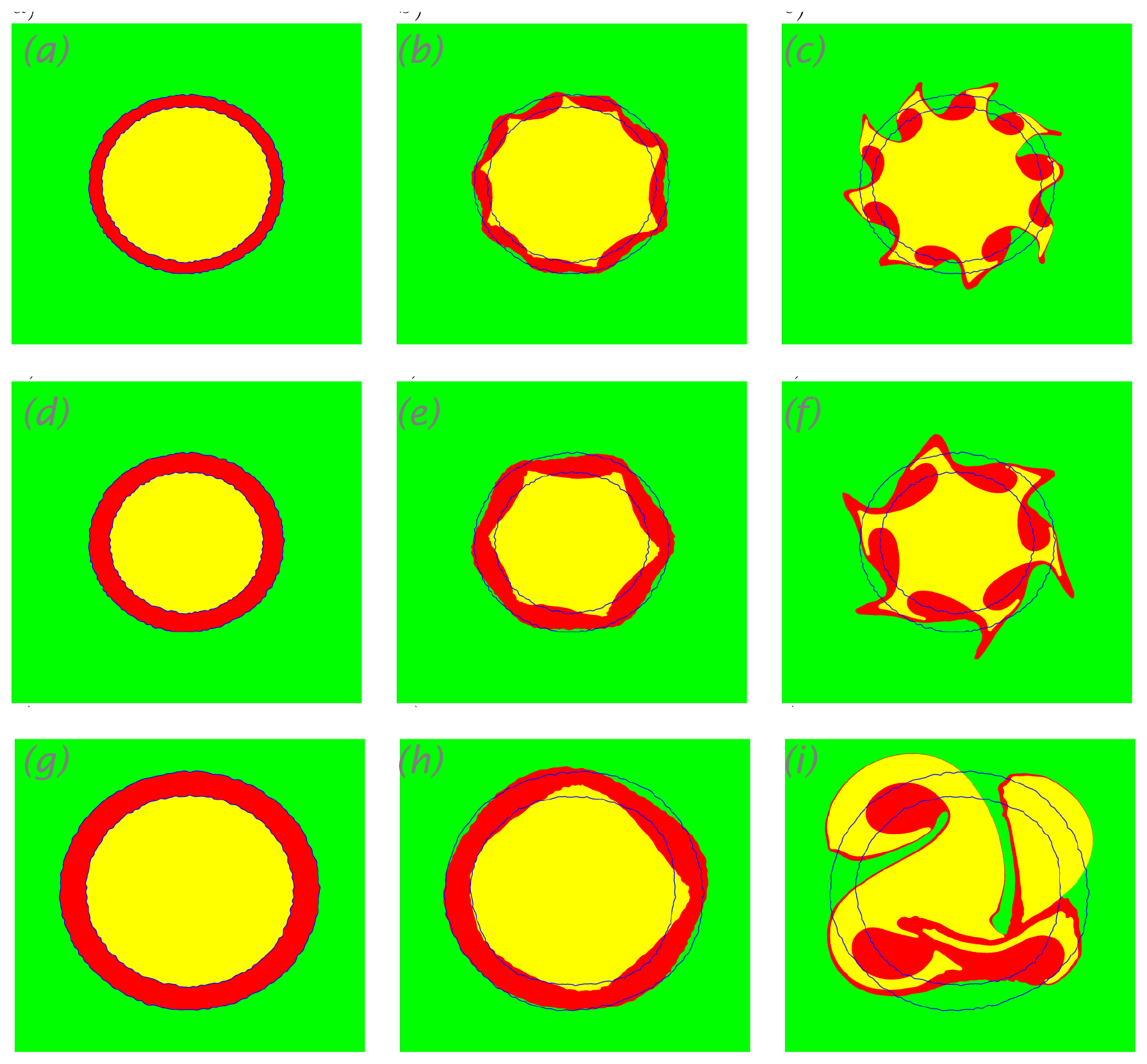
Figure 16 Evolution of three different annular bands subjected to initial small amplitude random perturbations. The initial states are shown in panels (a), (d), and (g) for which the external parameters ($a,b,C,n$) take the respective values of (0.434, 0.5, 1.71, −0.57), (0.4, 0.5, 1.12, −0.63), and (0.53, 0.67, 0.20, −0.65). In each case the jet strength is 120 m s⁻¹. Panels (b), (e), and (h) display an early quasi-linear development phase, and panels (c), (f), and (i) capture a mature non-linear phase.

Figure 17 shows an example of the evolution of an initial finite amplitude m = 2 perturbations of the r = b interface but with no perturbation of the inner (r = a) interface. This setting is that envisaged in the previous sub-section, and pertains for ($C,a,b,n$) = (1.0, 0.447, 0.5, −0.5) that again corresponds to a jet of 120 m s⁻¹ and perturbed by a wave with an amplitude of 0.03. Again, in harmony with the results derived earlier, the evolution exhibits a notable growth over a period of 3.2 d.

Figure 17 Development of an annular band's absolute vorticity when the outer interface (r=b) is subject to an initial finite-amplitude m=2 wave perturbation. The simulation is for $(a,b,C,n)$ taking the values (0.447, 0.5, 1.0, −0.5) with an initial wave amplitude of (0.03). Panel (a) displays an initial state, and the patterns displayed in panels (b) and (c) are in dimensional terms after 1.3 and 3.2 d.

It results in the formation of two vortex structures each possessing a trailing filamentary structure, and the pattern and its subsequent development (not shown) bears a modicum of resemblance to the split classification pattern that can emerge during an SSW event. However, the simplicity of our model cautions against overstating the relationship to realized events.

It is also pertinent to note the results of two null simulations of this case (not shown). First for an initial small amplitude random noise perturbation of both interfaces, there evolves the (expected according to our normal mode theory) growth of a wave number m=12. The second null simulation corresponds to an initial configuration comprising a jet of the same strength as before at r = b but now with a uniform absolute vorticity distribution across the entire r<b domain. When subjected to the same 0.03 amplitude wave perturbation at r=b, the configuration evolves to a steadily rotating ellipse with an aspect ratio close to unity. In effect, these “null” simulations indicate that the vortex breakdown is attributable explicitly to the existence of the annular band. This underlines and illustrates the significance of the results presented in Sect. 3.2.4, and points to the efficacy of the gravest-mode wave forcing to the break-up of an annular vortex.

3.5 Model Critique and Assessment of the Results

This study's examination of the possible barotropic instability of the Polar Night Jet was geared not to replicating (or refuting) the results of the previous numerous related studies but rather was aimed at seeking further understanding of the associated processes. Our results are constrained by the simplicity of the adopted polar β-plane configuration and non-divergent barotropic model, and here we first comment in turn upon these restrictions.

The polar β-plane is a reasonable assumption for flow features confined substantially to the polar and extra-tropical latitudes because the Coriolis effect is well represented at these latitudes. By way of comparison, for barotropic flow on the sphere: (a) the Circulation Theorem imposes an integral constraint on the net globally area averaged relative vorticity, and (b) the requirement of inertial/symmetric stability of an axisymmetric basic state the relative vorticity must also be zero at the equator. On a polar β-plane there is no à priori equivalent to the integral constraint whilst a condition of zero relative vorticity imposed at the β-plane's pseudo-equivalent of the equator (that is, r_c=1.4) would imply for our model that a state of (unlikely) neutrality to symmetric perturbations pertains in the entire region between b and r_c (in effect the surf zone). Our approach has been to select a basic state absolute vorticity profile that ensures a relatively quiescent inner region (i.e. Z_I=0, for r<a), a jet capable of spanning the range of observed values, and a value for the absolute vorticity in the outer region that is both consistent with inertial (as opposed to barotropic) stability and yields realistic values for the zonal velocity and/or the relative vorticity at our model's equivalent of the sub-tropics.

The impact of setting, Z_I=lC, is that the key Eqs. (10) and (11) are modified to the form,

$$\begin{array}{}\text{(18)}& {\displaystyle }{m}_{\mathrm{0}}=[\mathrm{2}-(l+n\left)\right]/\left[\mathit{\epsilon }\right(\mathrm{1}+\mathit{\mu }-l\left)\right]\text{(19)}& {\displaystyle }\mathit{\sigma }=\mathrm{1}/\mathrm{2}/C/\sqrt{\left[\left(\mathrm{1}-n\right)\left(\mathrm{1}-l\right)\left(\mathrm{1}-\mathit{\epsilon }\right)m\right]}\end{array}$$

In effect for l≪1 the changes are minor with a reduced growth rate. The reverse shear across the annulus attributed to the inner region inhibits the instability, and a similar effect was noted in a simpler setting by Dritschel (1989b).

The second constraint referred to above is the limitation of non-divergence and barotropy. This alleviated somewhat at stratopause elevations by the deductions presented in Sect. 2 that were based upon the character of the observed features. Paldor et al. (2021) provide a formal comparison of geostrophic, shallow water divergent and non-divergent representations of barotropic instability. In passing we again note that our earlier observational deductions render more challenging the specification of the barotropic “equivalent depth” as adopted in some shallow water instability studies (Matthewman and Esler, 2011; Sharkey et al., 2021). More fundamentally the assumption of barotropy excludes consideration of baroclinic (cf. Dickinson, 1973; Simmons, 1974) and mixed barotropic-baroclinic (cf. Manney and Randel, 1993) instability at these elevations. In mitigation we note that the monopole character of the PV features points to a barotropic-like instability mechanism.

Positively, in comparison with some other studies, our model does not invoke quasi-geostrophy (cf. Davies, 1981; Hartmann, 1983), incorporates an acceptable representation of the β-effect (cf. Dritschel, 1989b; Dritschel and Polvani, 1992). The adoption of the polar β-plane configuration, as opposed to spherical geometry (Hartmann, 1983; Michaelangeli and Zurek, 1987; Manney et al., 1988; Mitchell et al., 2021; Waugh, 2023) enables a simpler derivation and interpretation of analytical solutions for a wide range of relatively realistic basic states velocity fields. Also, our examination of the annular feature and its response to a large wave perturbation differs from that pursued by Matthewman and Esler (2011) who considered the development of a non-annular vortex to such forcing.

The dependency of the most unstable normal mode to the jet's strength and skewness and to the width of the annular region was noted earlier. More generally the linear normal mode analysis and the non-linear simulations indicate that, for a wide range of external parameters characterizing the model's jet structure, the modes of maximum growth possess space-time scales and structure consistent with that of the observed features. In effect barotropic instability provides an attractive mechanism to account for the observed sub-planetary scale features.

An apparent discrepancy is that our normal-mode graver modes ($m=\mathrm{1},\mathrm{2}$) are stable in contrast with their instability as detected by Hartmann (1983). This can be linked to the form of the basic state adopted by Hartmann that can comprise a second weaker annulus of enhanced PV in mid-latitudes. This latter structure introduces two possible additional modes of instability associated either with the second annulus (with a most unstable mode of high wavenumber) or with the broad region of diminished PV located between the two annuli (with a most unstable mode of low wavenumber). This association was noted by Hartmann. The equivalent for our model configuration is an annulus of reduced absolute vorticity with a jet located at r=a associated with (C−>−1; l−>−1; n≪1). Inspection of Eqs. (18) and (19) suggests, and direct evaluation of Δ (see Sect. 3.2.4) confirms, that the wavenumber m=2 can be unstable and possess a large growth rate. The interpretation is that this mode's instability is aided by the basic state flow component within the annulus that is attributable to the “shear-effect” of the highly non-quiescent inner region.

Clearly the existence of this unstable mode in an upper-stratospheric setting depends crucially on the presence of an annulus of reduced PV. The evidence for such a feature is meagre although an instantaneous N-S section at a given longitude might (incorrectly) attribute such a structure to the existence of a trailing streamer of high PV emanating from the core and present within the surf zone at that longitude.

4 Further Remarks

This study can be viewed as lending further credence to two assertions regarding the Stratospheric Polar Vortex. The first is that the vortex's periphery can be populated with distinctive and dynamically significant sub-planetary scale flow features. Their presence (DS24) and this study's more detailed description of their structure, temporal evolution and dynamics serves to augment and refine the well-established documentation of SPV's overall structure (see Waugh and Polvani, 2010; Schoeberl and Newman, 2015; Butchart, 2022).

The second is that there is merit in considering the dynamics of a jet-like barotropically unstable flow configuration comprising an annular band of enhanced absolute vorticity to help account for the character of the forementioned observed features. Our linear instability analysis of such a band indicates that, for a wide range of external parameters characterizing the model's jet structure, the readily calculated normal modes that yield maximum growth rates possess space-time scales and structure consistent with that of the observed features. In effect barotropic instability provides an attractive mechanism to account for the observed sub-planetary scale features. In contrast the model's gravest planetary-scale normal modes ($m=\mathrm{1},\mathrm{2}$) are shown to be stable and hence do not of themselves support a small amplitude instability hypothesis associated with SSW events.

In addition, the study relates to two other key themes of contemporary SPV studies. First, for mass and chemical composition budget studies and for dynamically studies, it has been customary to identify (albeit as noted earlier in diverse ways) the SPV's “edge”. The occurrence of sub-planetary scale features near the SPV's periphery, each associated with a distinctive flow feature, adds further complication to defining the “edge”. Therefore, it would appear appropriate to characterize the vortex's periphery as possibly comprising “a rim of finite-width, that is highly variable in both in space and time, and that corresponds to an annular or fragmented region of enhanced PV”.

As noted earlier, this study bears upon the dynamics of SSW events that result from strong planetary-scale Rossby-wave (m=1 or 2) forcing from below acting upon the SPV. Our model simulations depict the rapid break-up of an annular structure when subject to strong m=1 or 2 wave-perturbation of its outer rim. It is therefore attractive to conjecture that a PV annulus of the stratospheric polar vortex in conjunction with the forementioned planetary-scale wave forcing of its outer rim could facilitate the break of the SPV itself. In such a development, the vortex “break-down” would result, not from a displacement or splitting of the SPV's core at stratopause levels, but rather from the aggregation into one or two distinct isolated entities of the annular band's PV on the SPV's periphery. Our linear theory indicates that the rapidity of the break-up is in part favoured by a narrow annular band. However, direct observational corroboration of the conjecture is hampered in part by the almost ubiquitous presence of large deviations away from symmetric circumpolar flow of the SPV at stratopause levels.

The present study would benefit from more detailed reanalysis-based case studies that include an evaluation of the influence of the parent model's GWD parameterization at and above the stratopause. Likewise, it would be illuminating to perform numerical simulations with a primitive equation model possessing high horizontal and vertical spatial resolution of potentially unstable basic flow states (or realized atmospheric states) and undertaken with, and without, strong Rossby wave forcing from below.

Appendix A: Comparison of upper stratospheric PV features in two Reanalysis data sets

The veracity of Reanalysis data sets at upper stratospheric levels is constrained by the accuracy of the dynamics and non-parameterized physics of the parent assimilation models, the adequacy of the raw data used for the analysis, the fidelity of any upper level phenomenologically based sub-grid scale Gravity Wave Drag (GWD) parameterization scheme, and any ad hoc divergence damping scheme of the models. In so-far as the parameterized schemes are tuned to match the expected state of the upper atmosphere, they have an artefact element that might/could compensate for, or disguise, other physical effects.

The figures recorded in the main text were derived from ERA-Interim Reanalysis (Dee et al., 2011a, b). Here we compare this data set's representation of the present study's key flow features with the corresponding fields derived from the MERRA2 set (Gelaro et al., 2017). The two assimilation models have horizontal resolutions at polar-extratropical latitudes, number of vertical levels, and top-most level of respectively for ERA-Interim of (∼79 km, 60, 0.1 hPa), and for MERRA2 of (∼50 km, 72, 0.01 hPa). In addition, MERRA2 incorporates improved stratospheric temperature data, and there are significant differences (see S-RIP, 2022, in particular Tables 2.3 and 2.7) in the treatment of the uppermost levels.

In Figs. A1, A2 and A3 the PV patterns displayed respectively in Figs. 2a, c, e, f, g, 6a and 9 (left column) are set alongside the corresponding MERRA2 patterns. The choice of PV as the elected variable is appropriate since it involves both the rotational component of the velocity and the thermal field whilst avoiding the divergent wind component that can be/is influenced by the differing treatment of inertia-gravity waves at stratopause levels in the various Reanalysis fields.

The similarity of these seminal sub-planetary scale PV features in the ERA-Interim and MERRA2 is striking particularly considering the forementioned differences in the procedure for deriving the two Reanalyses. It testifies to the consistency of their representation of these key features and lends credence to their accuracy and to our adoption of the ERA-Interim data set.

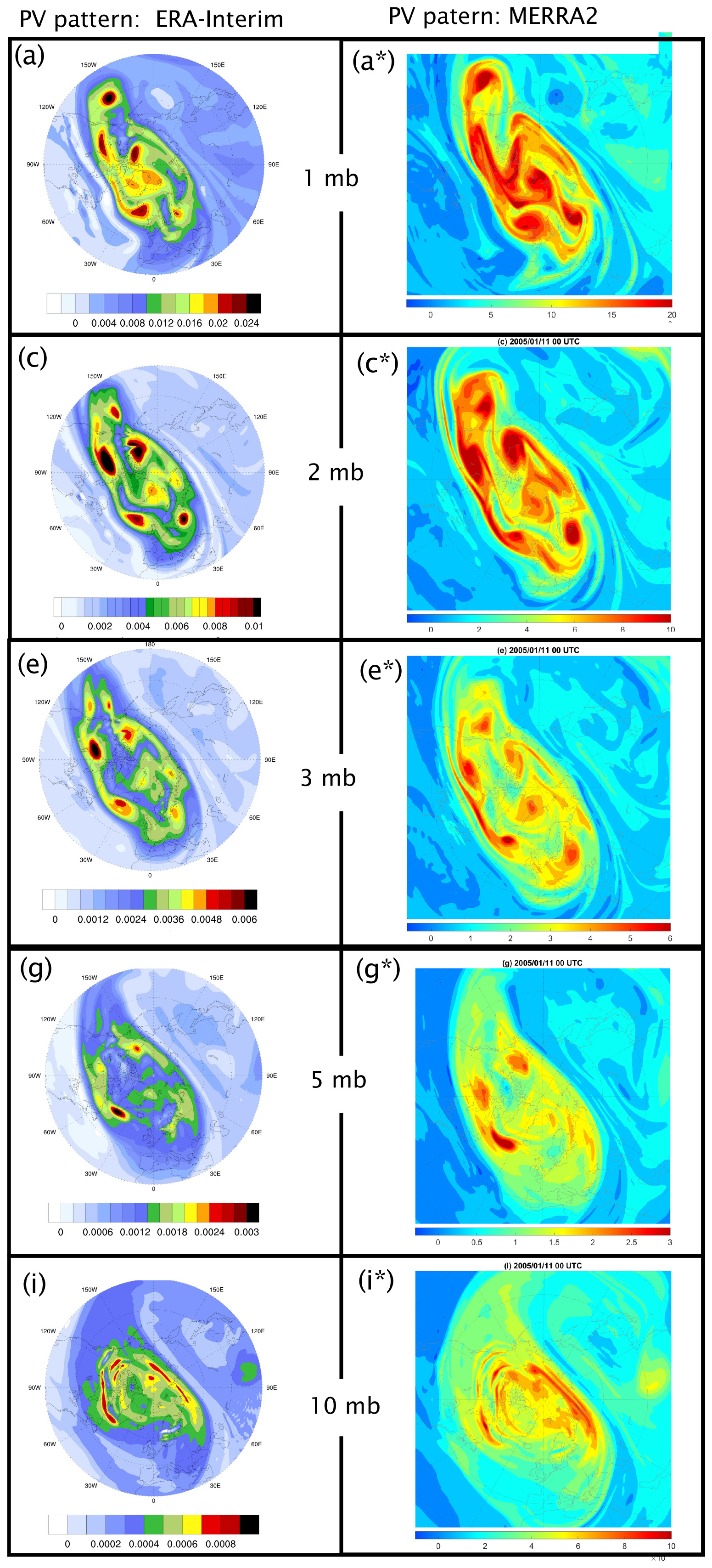
Figure A1 A comparison of the PV patterns derived with ECMWF-Interim data at 1, 2, 3, 5 and 10 mb. The left panels, Fig. 2a, c, e, g, i, are reproduced from the main text's Fig. 2, and in the right panels are the corresponding patterns derived from MERRA2 data. (Note the different colour scaling schemes for the two sets).

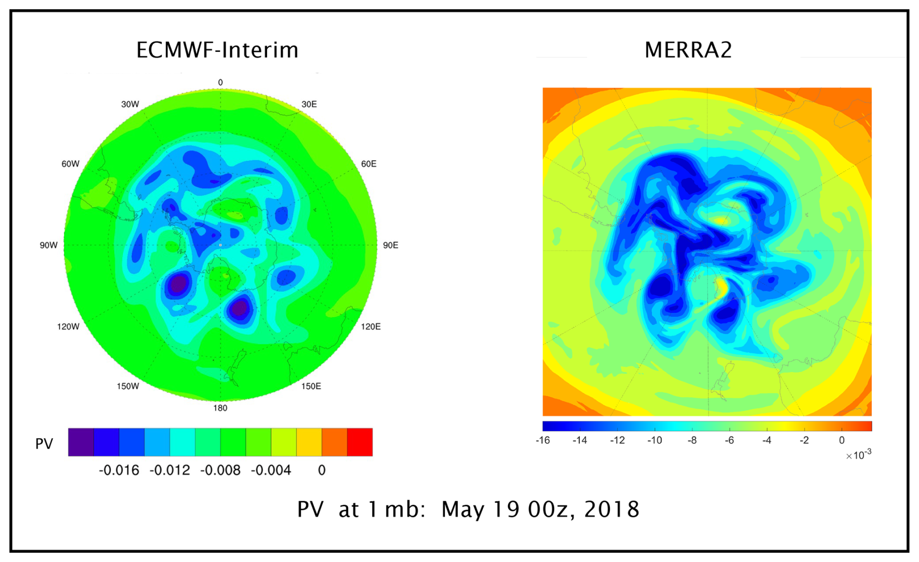
Figure A2 As for Fig. A1 but now comparing the PV pattern shown in Fig. 6a.

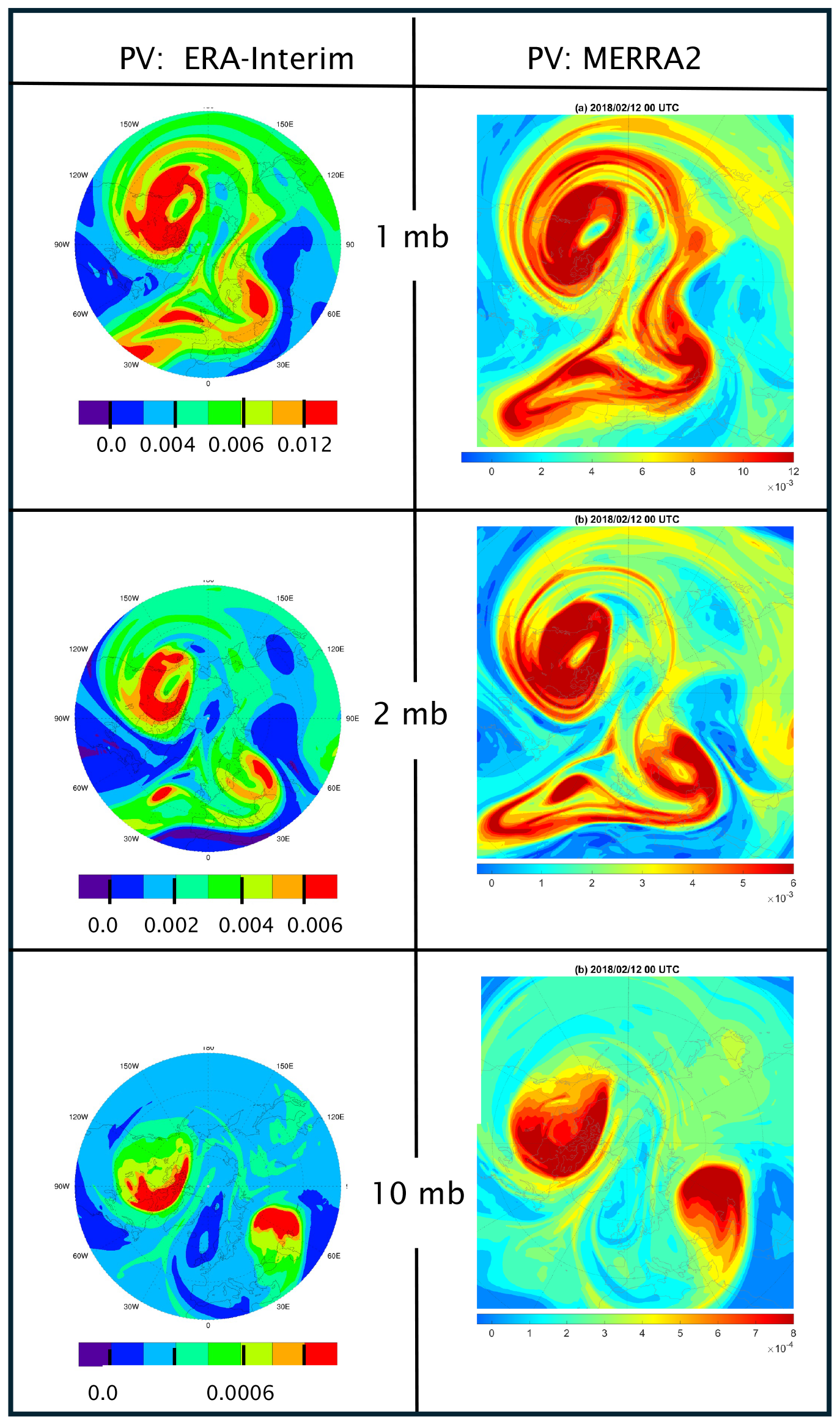
Figure A3 As for Fig. A1 but now comparing the PV pattern shown in Fig. 9.