Global monsoon in ICON: the scale-dependent response of Northern Hemisphere monsoons

The global monsoon system is a lifeline for two-thirds of the world's population, as it is essential for tropical water security, food, and agriculture. However, its complex multiscale interactions challenge weather and climate models. This study investigates how horizontal grid spacing (80, 40, and 10 km) in the ICOsahedral Non-hydrostatic (ICON) model affects both the mean and the variability of Northern Hemisphere monsoons across diurnal, intraseasonal, and interannual timescales. All simulations show substantial skill in capturing the global monsoon system domain and its mean annual range of precipitation with a pattern correlation of > 0.7 and RMSE < 3 mm d⁻¹. For the key Northern Hemisphere regional monsoons, South Asia (SAsiaM), West Africa (WAfriM) and North America (NAmerM), ICON achieves an accuracy > 80 % in capturing the observed monsoon domain. Crucially, the impact of grid spacing is strongly region-dependent and non-systematic. The finer grid spacing induces higher mean precipitation biases over continental SAsiaM, and WAfriM. Some of these biases are related to the intensity and location of moist monsoonal low-level jets, as well as their sensitivity to grid spacing. Furthermore, the fine grid spacing overestimates monsoon precipitation variability at interannual and intraseasonal scales, including intense precipitation frequency (> 10 mm d⁻¹). This amplification stems primarily from enhanced grid-scale precipitation resulting from efficient microphysical processes, while convective precipitation exhibits limited sensitivity to grid spacing. Over NAmerM, biases are smaller and show minimal sensitivity to model grid spacing. Increased intraseasonal variance (2–30 d band) in the 10 km simulation is linked to more intense low-pressure synoptic systems over SAsiaM and intense African easterly wave activity over WAfriM. All simulations agree on the diurnal precipitation peak timing, with the 10 km simulation marginally performing better over continents. Our results demonstrate that fine grid spacing alone does not uniformly improve monsoon simulations. Some features, such as the precipitation diurnal cycle, are improved while existing biases in mean precipitation and variability are enhanced. This underscores the role of region-dependent sensitivity of grid spacing governing monsoon dynamics.

1 Introduction

The global monsoon system encompasses the coupled dynamics of the ocean, atmosphere, land, and ice systems. It exhibits seasonal transitions of atmospheric circulation and precipitation driven by the annual solar cycle (Trenberth et al., 2000; Masson-Delmotte et al., 2021; Wang and Ding, 2008). Monsoon precipitation contributes to the livelihoods and agricultural productivity of more than 60 % of the world's population, particularly in tropical and subtropical regions. However, this rainfall undergoes significant changes on daily, seasonal, annual, and decadal timescales due to the influence of complex processes that interact across spatiotemporal scales of the earth system (Wang et al., 2014). The resulting variability in rainfall has profound impacts on agriculture, health, energy, and ecosystems, particularly in developing and vulnerable societies. Moreover, warming in the past century has perturbed monsoon systems by altering atmospheric circulation and intensifying precipitation extremes, thereby elevating the risks of both floods and droughts in monsoon regions (Zhang and Zhou, 2019; Singh et al., 2019). Given the critical role of the global monsoon system, it is essential to predict its associated variability and its governing processes.

Weather and climate models are very useful tools for simulating and predicting the monsoon system and its associated variability. However, complex spatio-temporal interactions ranging from large-scale global circulations to convective clusters make model simulations extremely challenging (Turner and Annamalai, 2012; Wang et al., 2017). Adding to this complexity, the global monsoon system is comprised of regional subsystems that undergo non-coherent variability on interdecadal to intraseasonal timescales, with some degree of interannual coherence driven by El Niño–Southern Oscillation (ENSO) (Geen et al., 2020). The Intergovernmental Panel on Climate Change Sixth Assessment Report on monsoons identifies six such subsystems: the South Asian (SAsiaM), East Asian (EAsiaM), Australian-Maritime Continent (AusMCM), West African (WAfriM), South American (SAmerM), and North American (NAmerM) monsoon systems, each featuring unique internal variability due to region-specific processes (Masson-Delmotte et al., 2021).

Studies based on data from the Coupled Model Intercomparison Project (CMIP) and Coordinated Regional Climate Downscaling Experiments (CORDEX) have made significant contributions towards understanding the global and regional monsoon dynamics and physics in present and future climate scenarios (Giorgi and Gutowski, 2015; Dunne et al., 2025; Eyring et al., 2016). Furthermore, ensemble weather and sub-seasonal-to-seasonal prediction systems have advanced in their monsoon forecasting skill (Pokhrel et al., 2016; Vellinga et al., 2013; Liu et al., 2014; Prein et al., 2022; O'Reilly et al., 2025; Saha et al., 2019; Nellipudi et al., 2026). However, these modeling systems typically operate at coarse grid spacing spanning tens to hundreds of kilometers. For example, the CMIP phase 6 models used horizontal grid spacings ranging from ≈ 0.7° (70 km) to 3.75° (300 km). Models operating at such coarse grids are challenged with under-resolved orography, simplified representation of key physics such as convection, turbulence and microphysics (Stevens et al., 2019).

The CMIP6 modeling community made substantial efforts to improve model physics and grid spacing to better resolve process interactions across spatiotemporal scales (Allan et al., 2023). Chen et al. (2024) investigated the representation of global monsoon and associated biases in CMIP6 compared to CMIP5 using an ensemble of 20 models. Their study reported a higher skill in simulating monsoon precipitation, intensity and the extent of monsoon domains in CMIP6, particularly for the Northern Hemisphere regions. However, despite these improvements, systematic biases, such as dry precipitation bias over Northern Hemisphere monsoon lands and an unrealistic oceanic extension of the monsoon domain, persist in CMIP6. A similar comparison over SAsiaM region by Choudhury et al. (2022) reported an improvement in the intensity and area covered by monsoon precipitation in CMIP6, but systematic dry biases over the continent and wet biases over the ocean persist. Further studies focusing on the SAsiaM and WAfriM regions reported persistent biases in CMIP6, with only minor improvements in the intensity of the precipitation dry bias (Katzenberger et al., 2021; He et al., 2023; Monerie et al., 2020).

Multi-model analysis from the High-Resolution Model Intercomparison Project (HighResMIP) with grid spacing ranging above 40 km reported improvements in SAsiaM monsoon precipitation biases compared to their coarse grid counterparts, especially over complex terrain (Li et al., 2025; Kumari et al., 2026). However, dry bias over central SAsiaM persisted but with reduced magnitude. The study concludes that the inherent design choices between models, such as the choice of model numerics and physics, remain a primary source of uncertainty, independent of grid spacing. Similar conclusions are also reported in regional CORDEX simulations (Choudhary et al., 2018; Ashfaq et al., 2021; Mishra et al., 2021; Pothapakula et al., 2020).

With increasing computational resources of High-Performance Computing (HPC) systems and investments in optimizing model code for modern hardware architectures, it is now possible to execute next-generation global models at unprecedented resolutions (Donahue et al., 2024; Dipankar et al., 2026; Prein et al., 2026; Paredes et al., 2023). These models have the potential to significantly improve the representation of tropical cyclones, land–sea interactions, inter-tropical convergence band, meso-scale convective systems, tropical waves, and Madden–Julian Oscillations (Stevens et al., 2019; Judt et al., 2021; Takasuka et al., 2024; Feng et al., 2025; Lee and Hohenegger, 2024; Segura et al., 2025; Kodama et al., 2021). However, challenges such as representing organized tropical convection or precipitation diurnal cycles over the ocean and land persist (Hohenegger et al., 2023; Segura et al., 2022; Feng et al., 2025). Furthermore, substantial computational resources required by fine grid spacing simulations limit the simulation length and ensemble size compared to their coarser counterparts, complicating model evaluation and climate change assessments.

The above inter-comparison studies show that the added value of decreasing grid spacing is region-dependent. While this result is to be expected as monsoon systems feature complex multi-scale interactions, a systematic study to understand how changing grid spacing affects rainfall in different monsoon regions is beneficial to advance the fundamental understanding of monsoonal flows and to guide future model development. Therefore, we conduct systematic grid spacing sensitivity experiments ranging from 80, 40, and 10 km with a single model. This hierarchy approximates the resolutions of CMIP-class models (Zhang et al., 2018), HighResMIP models, and CORDEX-type models. By keeping the model physics and dynamical constant, this design allows us to assess the effect of grid spacing on the monsoon system. For this, we leverage a refactored code of the ICOsahedral Non-hydrostatic (ICON) model developed with the Extreme-scale Computing and Data Platform for Cloud-Resolving Weather and Climate Modeling (EXCLAIM) project at ETH Zürich (Dipankar et al., 2026). The objective of our study is to (a) validate the representation of the global monsoon and its regional characteristics in ICON, and (b) to investigate its sensitivity to varying horizontal grid spacings concerning the representation of monsoonal mean state to interannual, intraseasonal to diurnal scales.

Specifically, we address the following questions:

• 1.

  Do ICON simulations capture the global monsoon domain and its mean precipitation and precipitation frequency distribution accurately?

• 2.

  How are the regional monsoonal characteristics, such as onset, interannual, intraseasonal and diurnal scales, represented?

• 3.

  Are the results sensitive to changing horizontal grid spacing? If so, what processes are responsible for this sensitivity?

In the following text, we briefly introduce the refactored version of ICON and the model setup, followed by methods used for analysis in Sect. 2. In Sect. 3, we show the ICON performance in capturing the spatial extent of the global monsoon, followed by its regional monsoon characteristics ranging from mean climate to diurnal scales. Finally, we conclude our remarks in Sect. 4.

2 Methodology

Section 2.1 outlines the ICON model, the experimental setup, and their computational implementation. Section 2.2 describes the observational references, verification metrics, and process-based diagnostics used to evaluate the model's performance in simulating the global monsoon domain, regional monsoon characteristics (including onset and extent), and mean precipitation, frequency and its variability across interannual to diurnal timescales.

2.1 Modeling

Recent advances in HPC systems have substantially improved the computational throughput of weather and climate models. We use the refactored ICON code described in Dipankar et al. (2026) that uses a GT4Py-based dynamical core developed within the EXCLAIM project. We performed global ICON experiments on the new ALPS HPC infrastructure of the Swiss National Computing Center at grid spacings of 80, 40, and 10 km from 2006–2016 including 1 year of spin-up. The 10 km simulation uses 32 Grace Hopper-200 GPU nodes, achieving a computational throughput of approximately 0.7 simulated years per wall clock day. The 40 km and 80 km run used 24 and 1 node, respectively, with throughputs of 5 and 4.9 simulated years per wall clock day. Initial conditions for all simulations are derived from European Center for Medium-Range Weather Forecasts (ECMWF) operational analysis on 1 November 2005, 00:00 UTC, with sea surface temperatures and sea ice data taken from Program for Climate Model Diagnosis and Intercomparison (PCMDI) AMIP II (Taylor et al., 2012). This boundary condition data is available at approximately 1° horizontal grid spacing and is updated monthly, with the ICON model performing a linear temporal interpolation to daily resolution.

The simulations use 120 vertical levels with a terrain-following hybrid setup based on smooth level vertical (SLEVE) coordinate (Leuenberger et al., 2010). The convection is parametrized using the Tiedtke–Bechtold bulk mass flux convection scheme, which treats shallow, mid, and deep convection with large-scale omega, boundary layer equilibrium, and convective available potential energy closure, respectively (Tiedtke, 1989; Bechtold et al., 2008). Cloud microphysics are calculated using a single-moment scheme for cloud water, cloud ice, snow, and rain (Doms et al., 2011). The turbulent kinetic energy-based surface transfer and planetary boundary layer parameterization are used for turbulence representation with a second-order closure (Raschendorfer et al., 2003). Land surface processes are simulated by the soil–vegetation–atmosphere-transfer submodel TERRA (Schulz and Vogel, 2020), which utilizes eight model levels and is responsible for exchanges of heat, moisture, and momentum. The TERRA uses a tile approach to account for the effects of subgrid surface heterogeneities (Avissar and Pielke, 1989).

A numerical time step of 60, 180, and 360 s is used for the 10, 40, and 80 km runs, respectively. The radiation scheme is called every 6 min. In contrast, the convection, cloud cover, sub-grid-scale orography, and non-orographic gravity wave drag schemes were called every time step in all simulations. The fast physics such as saturation adjustment, surface transfer scheme, land-surface scheme, boundary-layer/turbulent vertical diffusion scheme, and microphysics scheme are called every model timestep. The Tegen aerosols climatology (Tegen et al., 1997) is used, while Global and regional Earth-system Monitoring using Satellite and in-situ data (GEMS) and Monitoring Atmospheric Composition and Climate (MACC) ozone climatologies are used (Katragkou et al., 2015). The external parameters such as topography, land-use land cover, etc., required by ICON were prepared by the External Parameters for Numerical Weather Prediction and Climate Application software (Asensio et al., 2020). In Fig. S1 in the Supplement, we show the topography of SAsiaM, WAfriM, and NAmerM domains in various ICON simulations. The finer grid spacing resolves complex topographic structures such as the Himalayas, Western and Eastern Ghats of SAsiaM, Ethiopian Highlands of WAfriM, and the slopes of the Sierra Madre Occidental over NAmerM very well compared to its coarser grid counterparts (Fig. S2).

2.2 Validation and Analysis

We validate the ICON experiments across the global monsoon domain and the representation of its regional characteristics with an ensemble of gridded precipitation datasets shown in Table 1 for a period of 10 years (2007–2016). The precipitation observations include products derived from satellites, satellite observations corrected with in situ measurements, station-based, and reanalysis products. In addition to the precipitation, we use the Fifth-generation ECMWF Reanalysis (ERA5) data to verify the moisture transport (Hersbach et al., 2020). Furthermore, we utilize the Indian Meteorological database to validate monsoon low-pressure systems over the SAsiaM (Indian sub-continent) region. A detailed description of these datasets, including their advantages and limitations are provided in Appendix A.

Hersbach et al. (2020)Huffman et al. (2019)Beck et al. (2019)Helmi and Abdelhamed (2022)Xie and Arkin (1997)Schneider et al. (2014)Pai et al. (2014)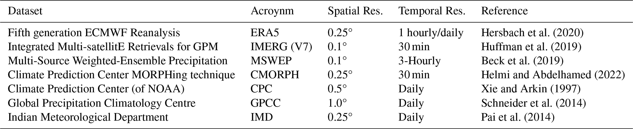

Table 1 Description of observational datasets.

To identify the global monsoon domain in observations and our simulations, we follow a standard definition from Wang and Ding (2008). First, we calculate the difference between local summer and local winter precipitation and identify regions that exceed 2 mm d⁻¹, and thereafter filter the regions where the contribution of local summer rainfall exceeds 55 % of total annual rainfall. Here, local summer is defined as June–July–August–September (JJAS) for the Northern Hemisphere and December–January–February–March (DJFM) for the Southern Hemisphere. The first criterion, i.e., the annual range (local summer minus winter) distinguishes the monsoon climatic regions from the equatorial perennial rainfall, while the second criterion (percentage of summer contribution) distinguishes monsoon from subtropical arid and semi-arid regimes. We use standard metrics such as spatial correlation and root mean square error to validate the annual range of precipitation over the global monsoon domain with observations.

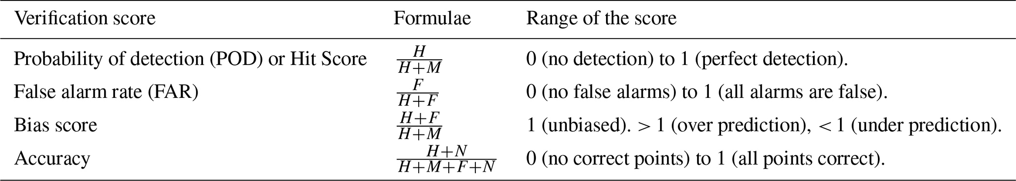
We use standard categorical verification metrics, such as the Probability of Detection (POD), False Alarm Ratio (FAR), bias score, and accuracy, to quantitatively assess ICON's skill in simulating regional monsoon domains (see Table 2).

Table 2 Definitions and interpretation of verification scores used to evaluate simulated monsoon domains. The H refers to hits, i.e., the number of grid points where ICON and observations agree to be a monsoon grid point (model YES, obs YES). The M refers to the observed monsoon points that the model misses (model NO, obs YES). The model predicted monsoon points not present in observations (model YES, obs NO) is referred to as False alarm (F), and correct negatives (N) are the points where both model and observation agree of a non-monsoon grid point.

Monsoon onset is a key metric impacting sectoral planning across all monsoon regions. We identify monsoon onset as the first date, after 1 March in the northern hemisphere and 1 November in the southern hemisphere, on which the pentad-mean (5 d running mean) precipitation exceeds 5 mm d⁻¹ for at least three consecutive pentads. This criterion accounts for transient events and follows the definition of Wang and LinHo (2002). Furthermore, Nguyen-Le (2023) tested various monsoon onset criteria across regional monsoon domains, and concluded that the methodology by Wang and LinHo (2002) agrees well with the observations.

The precipitation over various monsoon domains is largely fed by moist low-level jets advected from the oceans. Hence, we quantify the vertically integrated horizontal moisture transport in the lower troposphere from the surface to 850 hPa,

$$\begin{array}{}\text{(1)}& \mathit{Q}={\displaystyle \frac{\mathrm{1}}{g}}\underset{p_{\mathrm{sfc}}}{\overset{p_{\mathrm{850}\mathrm{hPa}}}{\int }}\mathit{V}q\mathrm{d}p,\end{array}$$

where Q is the moisture transport vector (kg ms⁻¹), g is the gravitational acceleration (m s⁻²), V is the wind vector (m s⁻¹), and q is the water vapor mixing ratio (kg kg⁻¹). The integration is performed from the model surface pressure (p_sfc) to 850 hPa. Over elevated terrain where p_sfc < 850 hPa, the layer has zero thickness and Q is not computed. We therefore restrict our analysis of low-level jets to oceanic and low-terrain regions, following Tamoffo et al. (2023).

2.2.1 Variability Across Timescales

Before analyzing monsoon variability across temporal scales, we first evaluate whether ICON faithfully replicates the distribution of daily precipitation intensities. We examine the cumulative distribution function (CDF) and probability of exceedance of daily precipitation rates across the core monsoon regions to assess the model's performance in capturing the observed frequency of light, moderate, and heavy rainfall events (Ban et al., 2014). We define light to medium precipitation as 1–10 mm d⁻¹, encompassing the high-frequency, mostly non-convective rainfall regime. Events > 10 mm d⁻¹, which often involve organized convection, are analyzed as the heavier intensity spectrum. The CDFs are computed using logarithmically spaced bins from 0.1 to 500 mm d⁻¹ during the local monsoon season. To explicitly assess the frequency of light-to-moderate precipitation, we analyze the CDF directly. To isolate biases in the extreme tail of the distribution, we analyze the complementary cumulative distribution function, or probability of exceedance (1−CDF). This dual representation allows for a clear comparison of the full intensity spectrum across models and observations.

Next, we quantify monsoon precipitation variance across interannual, intraseasonal, and diurnal timescales in ICON simulations and observations, and investigate its sensitivity to model grid spacing. Interannual variability is calculated as the variance of the annual mean local summer monsoon seasonal precipitation over the 10-year analysis period. Intraseasonal variability is separated into low-frequency (30–90 d) and high-frequency (2–30 d) bands using a 4th-order, zero-phase-shift Butterworth band-pass filter (Russell, 2006). The 30–90 d band primarily is associated with the Madden–Julian Oscillation, while the 2–30 d band isolates variability associated with synoptic-scale systems such as monsoon lows and tropical waves. Variance is calculated separately for each filtered time series.

We investigate the key processes associated with the synoptic-scale intraseasonal band in the SAsiaM and WAfriM regions contributing to precipitation variance. For the SAsiaM region, we track Synoptic Low Pressure Systems (LPS) often referred to as the monsoon lows, depressions (D) or deep depressions (DD), cyclonic storms (CS) and severe cyclonic storms (SCS) as defined by the Indian Meteorological Department (Hunt et al., 2016; Sikka, 2006). For WAfriM, we first examine the vertical structure of the African Easterly Jet and Tropical Easterly Jet in simulations and reanalysis. We then use the variance of band-pass filtered (2–10 d) daily meridional wind as a proxy for African Easterly Wave (AEW) activity, which is linked to organized convection (Nicholson and Grist, 2003; Tamoffo et al., 2023).

Diurnal variability is analyzed by first computing the mean diurnal cycle of hourly precipitation during the local monsoon season (JJAS for the Northern Hemisphere). The diurnal peak timing is then identified as the hour of maximum precipitation in local solar time.

2.2.2 Tracking Synoptic Low Pressure Systems

We developed an automated tracker to detect monsoon LPS over SAsiaM. We particularly focus on systems originating over the Northern Indian Ocean (Bay of Bengal) and moving towards the land, contributing to significant precipitation, and in some cases extreme rainfall over the Indian sub-continent. LPSs are identified using mean sea-level pressure (MSLP) and horizontal wind components (u,v) at 850 hPa, extracted from the ERA5 reanalysis and ICON simulations. Tracking is performed at 6-hourly intervals to ensure temporal consistency across datasets. We followed the study of Vishnu et al. (2020) in choosing the thresholds for detecting the LPS.

In the first step, the tracker identifies LPS centers where the Laplacian exceeds 3.0 hPa, calculated over the immediate neighbors of the grid cell. Next, we calculate the stream function (ψ) from the 850 hPa wind field using the u and v components. To isolate synoptic-scale vorticity features and suppress grid-scale noise, we apply a two-dimensional Gaussian spatial filter to the 850 hPa stream function field. The filter uses a standard deviation of σ = 150 km, which effectively smooths features smaller than approximately ≈ 300–400 km (≈ 2 σ–3 σ), consistent with the scale of monsoon low-pressure systems. This pre-processing step follows the methodology of Vishnu et al. (2020). The LPS candidates are retained only if their associated normalized stream-function amplitude exceeds ψ ≥ 0.2 σ, ensuring a robust, smoothed vorticity signature. Next, the tracker connects LPS candidates in time if their locations are less than 250 km apart, corresponding to a maximum movement speed of ≤ 50 km h⁻¹ in 6 h, while restricting the turning angle to 120° to ensure physically plausible LPS trajectories and avoid spurious connections.

We remove LPS that live for less than 24 h or have a minimum central pressure at the time of genesis (first detection) greater than 1005 hPa. Genesis points are required to occur over the Bay of Bengal (5–22° N, 80–97° E), and any centers detected over land are eliminated; thus we focus on LPS's originating over ocean and moving northwestward toward the land. Also, we considered only LPSs that make landfall over India. The final LPS tracks from the tracker are compared against subjectively analyzed best-track data from the India Meteorological Department (IMD). Finally, we categorized the tracked LPS based on the strength of the maximum 10 m wind speed it attains during its lifetime, following the criteria of IMD (Sikka, 2006).

3 Results and Discussion

In this section, we evaluate the skill of the ICON simulations and their sensitivity to grid spacing against observational datasets and the ERA5 reanalysis. We begin by examining the model's ability to capture the global monsoon domain, followed by a detailed investigation of its regional characteristics. Thereafter, we focus on regional analysis, investigating monsoon onset, precipitation patterns and their interannual and intraseasonal variance, the diurnal cycle characteristics, and precipitation frequency distributions. Finally, to understand the processes governing the simulated synoptic variability contributing to the intraseasonal variance, we focus on two key monsoon regions: over the SAsiaM domain we investigate the characteristics of monsoon LPS, and over the WAfriM domain we investigate the African Easterly Wave activity.

3.1 Representation and Skill of Monsoon Domains in ICON Simulations

We delineated the global monsoon domain using the criteria of Wang and Ding (2008) in our ICON grid spacing runs and in the IMERG reference dataset (Fig. 1a–d). The contours mark the monsoon boundaries, while the shading depicts the annual range (local summer minus winter), a key metric of monsoon intensity. All ICON simulations broadly capture the spatial pattern of the monsoon domains representing the well-known monsoon regions such as the NAmerM, SAmerM, WAfriM, SAsiaM, EAsiaM, AusMCM, SAfriM, including their adjacent oceans (Masson-Delmotte et al., 2021).

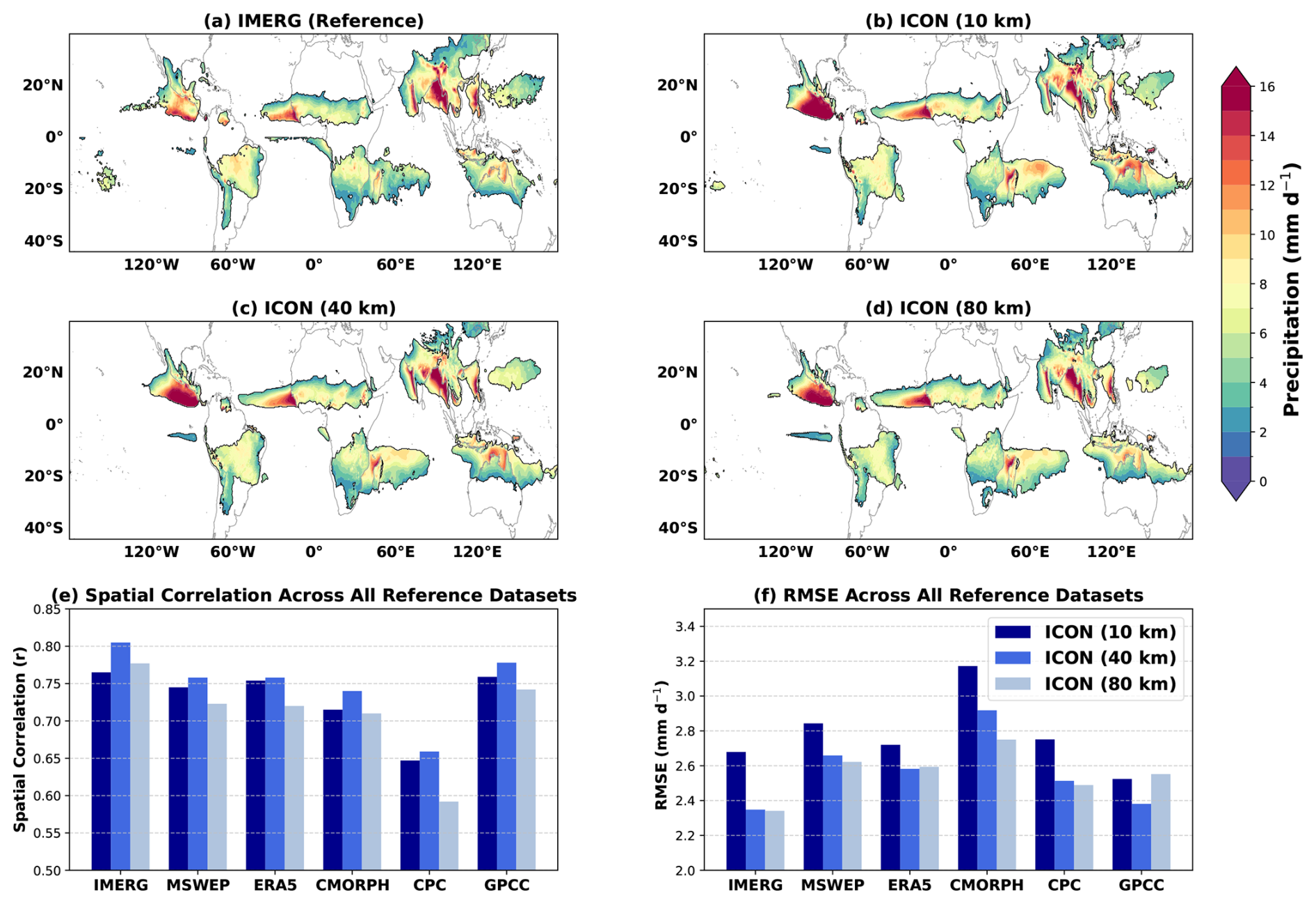
Figure 1 Global monsoon domains (contours), defined by regions where local summer minus winter precipitation difference is > 2 mm d⁻¹ and summer precipitation contribution is ≥ 55 % of annual total. The shaded regions show the annual range of precipitation (local summer minus winter) in (a) IMERG observations and (b–d) ICON simulations at 10, 40, and 80 km grid spacing. (e) Spatial correlation and (f) RMSE of the monsoon precipitation annual range for ICON simulations against six observational datasets (2007–2016). The spatial correlation and RMSE values are statistically significant with p < 0.05 based on a two-sided Student's t test. All the datasets are plotted and analyzed at a common grid close to ERA5 with a grid spacing of about 30 km.

The IMERG data shows the most intense annual range in monsoon precipitation over the SAsiaM domain, with values exceeding 14 mm d⁻¹ over the head Bay of Bengal, the eastern Arabian Sea, the western Pacific, and the orographically dominated regions of the Himalayas and Western Ghats. All the ICON simulations broadly capture these features. A notable resolution dependence is evident over the Himalayan foothills, where only the highest-resolution (10 km) simulation reproduces the magnitude observed in IMERG, while the 40 and 80 km runs are unable to replicate the orographically induced precipitation pattern. Furthermore, while all simulations capture the annual range maximum over the continental core of the Indian monsoon region, they consistently show a slight overestimation in this area. All ICON simulations reproduce the core EAsiaM domain and its general annual precipitation range. However, they exhibit a systematic bias in capturing the full spatial extent of the monsoon domain along its northwestern margin, specifically the transitional zone bordering the Tibetan Plateau and continental China.

Over the WAfriM domain, IMERG shows a large annual range (> 12 mm d⁻¹) over the eastern tropical Atlantic, off the coast of Guinea. Across the continental interior, a north-south gradient characterizes the monsoon, with the maximum annual range is visible in the southern part of the domain. All the simulations overestimate both the spatial extent and the annual range over the tropical Atlantic. However, the continental spatial patterns, i.e., the north-south gradient, are broadly captured well in all simulations. For the NAmerM domain, IMERG shows a peak annual range (> 12 mm d⁻¹) over the equatorial eastern Pacific Ocean, followed by a secondary continental peak over northwestern Mexico and the southwestern United States, marking the core monsoon region. All ICON simulations consistently overestimate the annual range over the equatorial eastern Pacific Ocean. While the general features over the continent are captured, the spatial extent of the domain is underestimated, particularly near the interior western United States, and southeastern Mexico.

In the Southern Hemisphere region, IMERG shows peak annual range (> 10 mm d⁻¹) over the southern Pacific ocean, off the coast of northern Australia, followed by the southern Indian ocean, off the coast of South Africa. All simulations show a consistent overestimation of the annual range over these oceanic regions, with a larger magnitude in the finest-grid (10 km) simulation. Over the continental regions of SAmerM, SAfriM and AusMCM, all simulations align well with the IMERG reference data. All the qualitative results presented above remain robust when evaluated against an ensemble of observational datasets (MSWEP, CMORPH, ERA5, GPCC, and CPC; see Table 1 and Fig. S3).

We quantified model performance using the spatial correlation coefficient and root-mean-square error of annual precipitation range, comparing the ICON simulations with an ensemble of reference datasets to account for observational uncertainty. For the global monsoon domain, all ICON simulations show significant spatial correlations (> 0.7) with all observational datasets (except CPC, a land-only in situ dataset), indicating a robust representation of the spatial precipitation pattern. The 10 and 40 km runs consistently showed greater correlations than the 80 km simulation (except for the 10 km compared to IMERG).

Regarding the RMSE, the 10 km simulation produces the highest values (> 2.5 mm d⁻¹) across all observational datasets, exceeding those of the 40 and 80 km runs. Analysis of the error distribution (Fig. S4) reveals that the elevated RMSE largely stems from the greater annual range over oceanic regions, suggesting greater sensitivity of simulated oceanic precipitation to model grid spacing. Furthermore, to assess the uncertainty associated with the grid remapping methodology, we also performed the analysis on a common coarse grid of 80 km spacing. As shown in Fig. S5, the qualitative conclusions remain unchanged, confirming the robustness of our results.

We next assess the representation of regional monsoon characteristics by examining the monsoon domains and local summer precipitation for each major regional system (Fig. 2a–f). For the purposes of this article, we focus on tropical monsoon systems in the Northern Hemisphere, but we show a preliminary investigation of monsoon domain spatial extent from various ICON simulations for Southern Hemisphere monsoons. A detailed investigation of the characteristics of Southern Hemisphere monsoons is, however, beyond the scope of this article. The black contours represent the IMERG reference, and the red, green, and blue contours represent the 10, 40, and 80 km grid spacing runs regional monsoon boundaries, respectively, while the shading represents the observed IMERG local summer precipitation. Over the combined SAsiaM/EAsiaM region, all simulations broadly capture the IMERG monsoon domain. However, all simulations exhibit a systematic bias in capturing the full spatial extent of monsoon domain along key margins. Specifically, the transitional zone connecting the western Pacific coastal basins to the deep ocean near 120° E, and the inland boundary bordering the Tibetan Plateau and continental China. Quantitative verification scores for the monsoon domain, including the hit rate, false alarm ratio, bias, and accuracy, are shown in Figs. S6–S8 for various observational datasets. All runs show high-quality, consistent performance (e.g., accuracy ≈ 0.85), indicating reliable monsoon domain detection in all simulations. The spatial pattern of IMERG local summer monsoon precipitation largely follows that of the annual range shown in Fig. 1, confirming the dominance of summer precipitation in delineating the monsoon seasonal signal.

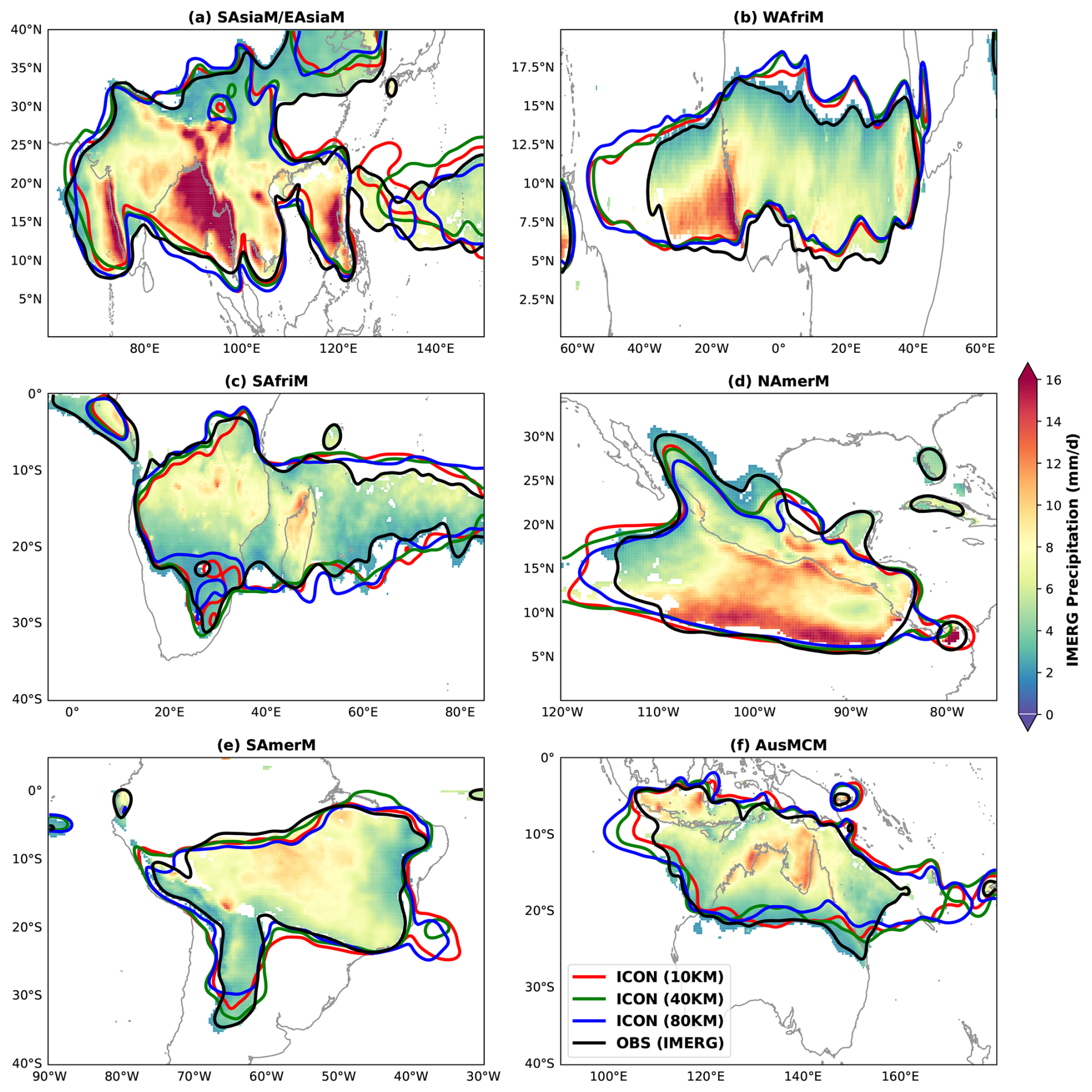
Figure 2 Regional monsoon domains (a) SAsia/EAsiaM (b) WAfriM (c) SAfriM (d) NAmerM (e) SAmerM (f) AusMCM detected in various ICON simulations and IMERG reference dataset defined as the regions where the local summer minus winter precipitation is > 2 mm d⁻¹ and summer contribution is ≥ 55 % of annual total. The black contours show monsoon domains in IMERG observational dataset, while the red, blue, green show the boundaries for 10, 40, 80 km simulations respectively. The shading shows the total precipitation in mm d⁻¹ (local summer) from IMERG reference dataset. Contours are Gaussian-smoothed (σ = 3) for clarity.

For the WAfriM domain, all simulations show an extended monsoon domain over the Atlantic Ocean, off the coast of Guinea, and a slight northward shift toward the Sahara. This misalignment results in a slightly higher FAR of > 20 % compared to other monsoon domains. However, all ICON runs show high scores (e.g., accuracy > 0.82), with a slight added value in 10 km simulation compared to 40 and 80 km. Over the NAmerM domain, almost all the ICON simulations are unable to capture the full inland of continental southern United States, specifically towards the northern and the eastern boundaries compared to IMERG. Furthermore, an overestimation of the equatorial Pacific Ocean is detected. Nevertheless, again the verification scores for the NAmerM remain high, with an accuracy of ≈ 0.85. The summer monsoon precipitation patterns for both NAmerM and WAfriM domains again broadly follow the spatial patterns of the annual range precipitation.

Overall, for detecting regional monsoon domain metrics, we conclude that all ICON runs show robust, high quality results independent of grid spacing. Furthermore, these findings are consistent across observational datasets, confirming their robustness.

3.2 Monsoon Onset Characteristics

Onset timing, progression and direction are some primary characteristics of monsoon systems, hence their reliable representation in the model is essential. Figure 3 shows the monsoon onset in IMERG compared to our ICON runs for the SAsiaM (a–d), WAfriM (e–h), and NAmerM (i–l) domains. IMERG shows a characteristic southeast-to-northwest propagation of the SAsiaM, with the progression beginning over the Bay of Bengal, the southeast Arabian Sea off the coast of Eastern Ghats in late April, and then progressing towards the continental northwest Indian continent by the end of June. An early onset signal in March over the foothills of the Himalayas and near Bangladesh is likely due to persistent orographic rainfall interacting with the low-level monsoon flow. Within this domain, the EAsiaM also follows a southeast to northwest progression from continental China towards the Tibetan Plateau. The IMERG results agree well with the general propagation features of the monsoon (Nguyen-Le, 2023), confirming the reliability of our monsoon onset definition. All the ICON simulations capture the large-scale propagation features, but with notable discrepancies. For example, they exhibit a delayed and less homogeneous progression over the Bay of Bengal, and the 80 km run show a delayed onset over central India compared to fine-grid spacing runs. Furthermore, all runs are unable to capture the inland propagation over continental China, consistent with their unrealistic representation of the EAsiaM rainfall domain (Fig. 2a).

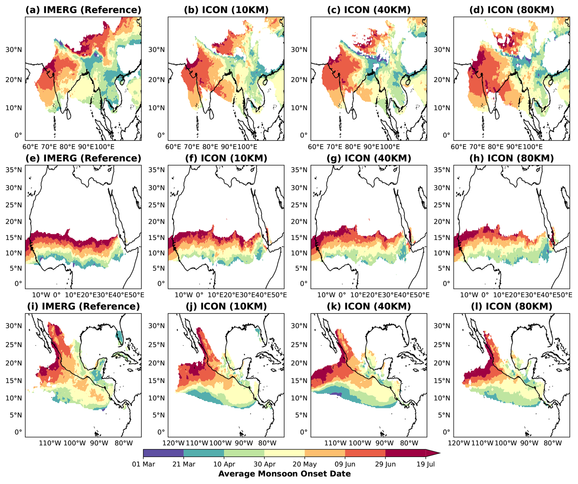
Figure 3 Spatial patterns of monsoon onset dates over the (a–d) SAsiaM, (e–h) WAfriM and the (i–l) NAmerM domain in IMERG and ICON simulations. The onset of a monsoon is defined as the first day starting from March, on which pentad-mean (5 d running mean) precipitation exceeds 5 mm d⁻¹ for at least three consecutive pentads. The definition of the monsoon onset is consistent across various monsoon domains to ensure the property of universal applicability.

The WAfriM domain features a northward propagation primarily linked to the movement of the Intertropical Convergence Zone (ITCZ), and local land–atmosphere feedbacks. The progression begins in late March to early April near the Guinea region, advances into the Sudanian region by late April to May, and finally reaches the Sahel region by June–July. All simulations capture this large-scale feature. The IMERG onset progression within the NAmerM domain shows two distinct regimes: (1) an early April–May onset over southeastern Mexico and the adjacent western Caribbean, associated with the northward migration of the ITCZ and the bimodal rainfall pattern of Central America, and (2) the canonical late June–July onset of the core North American Monsoon. The core monsoon onset is characterized by a northwestward progression of organized convection from the eastern Pacific Ocean into the Sierra Madre Occidental of northwestern Mexico and the southwestern United States (e.g., Adams and Comrie, 1997; Wayne Higgins et al., 2003). All simulations capture the progression of the NAmerM from the eastern Pacific to the southwestern United States. However, the inland penetration of the NAmerM into the southern United States is absent (Fig. 2d).

While the large-scale patterns of the monsoon onset are well captured in ICON runs, they exhibit some systematic biases in timing. In Fig. 4, we show the onset biases (ICON minus IMERG), along with a statistical investigation of errors over the core monsoon domains using violin plots. Over the SAsiaM domain (Fig. 4a–d), two major large scale biases emerge in all runs: (1) a systematic late onset (≈ 10–20 d) over continental southeast Asia, Bay of Bengal, and continental central India suggesting a delay in the model's representation of the monsoon trough's northward progression and associated moisture convergence (2) an early onset (≈ 30–40 d) over the Himalayas, Tibetan Plateau and continental China, a common bias often linked to unrealistic snow representation, excessive springtime heating and spurious convection over complex topography (Senan et al., 2016). The improvement with finer grid spacing is not systematic across all regions. While the early onset over the Tibetan Plateau is partially reduced in the 10 km run, the delayed onset over southern India is smallest in the 40 km run. Over the core monsoon region, the median (mean) delayed onset for ICON 10, 40, and 80 km are 7 (7), 3 (5), and 12 (12) d, respectively. This indicates that the 10 and 40 km run marginally improve the onset bias compared to 80 km. The difference in the onset bias is very small between 10 and 40 km grid spacings highlighting a non-monotonic relationship with grid spacing.

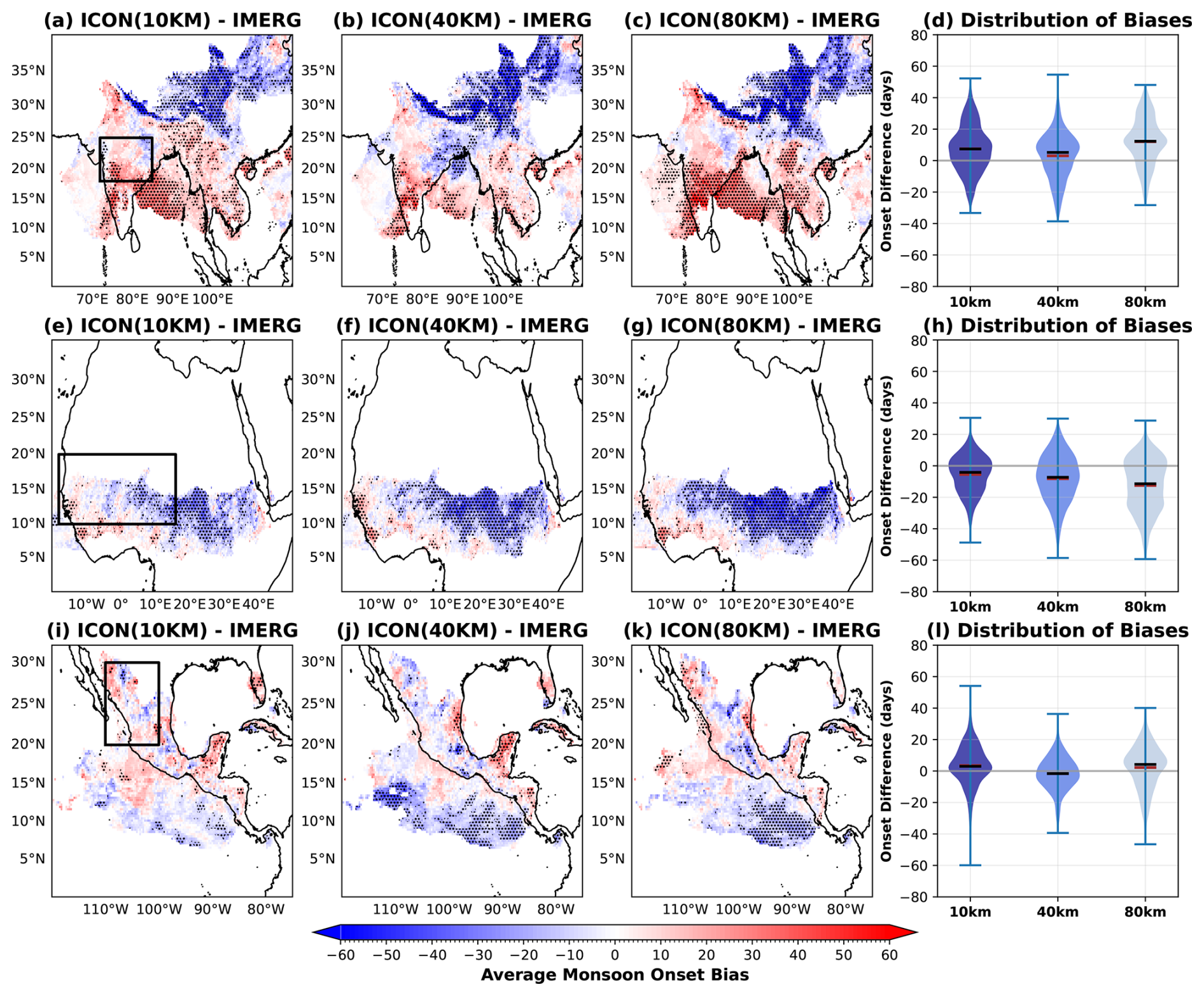
Figure 4 Spatial patterns of mean bias in the monsoon onset during the summer monsoon season (JJAS) in various simulations with reference to IMERG dataset for (a–d) the SAsiaM domain, (e–h) WAfriM, and (i–l) NAmerM. Stippling indicates grid points where the onset bias is statistically significant at the 95 % confidence level based on a two-sided Student's t test. The black boxes in the SAsiaM (a), WAfriM (e) and NAmerM (i) domains indicate the respective core monsoon regions, and the violin plots show the bias distribution of the monsoon onset day over the highlighted box regions. The black bar in the violin plots indicate the median, while the brown bar indicates the mean bias in monsoon onset over the monsoon core regions.

Over the WAfriM (Fig. 4e–h) domain, all runs show a systematic early-onset bias (≈ 20–30 d) over the eastern Sahel and Sudanian region, that might be related to land-atmosphere feedback errors in these interior zones. This bias is systematically reduced with finer grid spacing. In contrast, over the western African coast and the adjacent eastern Atlantic, all simulations show substantially smaller biases compared to the eastern continental regions, suggesting model performance is more constrained by observed oceanic boundary conditions. Over the core monsoon region, the 10, 40, and 80 km runs show a median (mean) early onset bias of 6 (4), 8 (7), and 10 (11) d respectively, representing a systematic improvement of ≈ 60 % for the 10 km run compared to the 80 km simulation. Furthermore, the bimodal (double-peak) bias distribution evident in the 80 km simulation (Fig. 4h), indicating two distinct bias patterns, is consolidated into a single, sharper peak in the 10 km run. This showcases a marginal improvement in the representation of monsoon onset characteristics with fine grid spacing over WAfriM.

The bias patterns over the NAmerM domain (Fig. 4i–l) are less coherent, underscoring the challenge of representing the intricate dynamic and thermodynamic processes that govern it. Despite this complexity, a clear non-monotonic grid spacing dependence emerges in the core monsoon region. The 40 km run shows the best performance with a minimal median (mean) early bias of −2 (−2) d. On the contrary, both the 10 and 80 km runs exhibit a delayed onset, with biases of 3 (3) and 2 (4) d, respectively. This result suggests that while coarse resolution (80 km) is insufficient to capture key onset dynamics, the highest resolution (10 km) may potentially introduce its own biases that require further investigation. Overall, the mean biases for NAmerM are notably smaller in magnitude than those for the SAsiaM and WAfriM domains.

In summary, results reveal that ICON reliably captures the large-scale onset characteristics but exhibits region-dependent biases that are modulated by model grid spacing in non-systematic ways. For the WAfriM, finer grid spacing yields marginal improvement. However, for the SAsiaM and NAmerM, the relationship is non-monotonic. The overall magnitude of onset timing biases is smallest for the NAmerM, followed by the WAfriM. These results remain qualitatively consistent when validated against CMORPH, ERA5 and MSWEP (shown in Fig. S9). All ICON simulations use monthly SST data linearly interpolated to daily resolution. Sensitivity experiments with a daily high-resolution SST product reveal that monsoon onset over SAsiaM and WAfriM is sensitive to SST bias and update frequency. Nevertheless, since all grid spacing experiments (10–80 km) use identical SST boundary conditions, our conclusions about grid spacing remain robust.

3.3 Monsoon Precipitation Characteristics and Associated Biases

Accurate representation of the spatial patterns and magnitude of monsoon precipitation has been a long-standing challenge for weather/climate models. Here, we investigate the precipitation features of the SAsiaM, WAfriM, and NAmerM domains and their associated biases.

Figure 5 Spatial patterns of the mean precipitation (mm d⁻¹) occurring during the summer monsoon season (JJAS) in reference IMERG and various ICON model simulations over the (a–d) SAsiaM domain, the (e–h) WAfriM, and the (i–l) NAmerM domains respectively. All the ICON simulations are brought to a common ERA5 grid (30 km) for fair comparison, and only the precipitation over monsoon domains as identified in Fig. 2 are shown.

Figure 5a–d show monsoon precipitation over the SAsiaM during local summer. IMERG shows peak precipitation (> 15 mm d⁻¹) over the head Bay of Bengal, the Himalayan foothills and Western Ghats, and over the south China/west Philippines Sea. Over the agriculturally critical central Indian core region, precipitation reaches ≈ 11 mm d⁻¹. A characteristic coastal maximum with subdued inland rainfall is also evident in the EAsiaM sub-region. All simulations reproduce the observed spatial patterns of these precipitation peaks. However, they exhibit region specific differences indicating resolution sensitivity. Most notably, only the 10 km simulation reproduces the observed IMERG precipitation peak over the Himalayan foothills, underscoring the need of a fine scale orography for realistic orography rainfall. Notably, all the runs capture the precipitation peak over the SAsiaM core region, indicating a reliable process representation in ICON such as the inland moisture transport, monsoon LPS, active/break oscillations and local land-atmosphere coupling. Across the EAsiaM region, the 10 km run also better captures the coastal to inland precipitation gradient, indicating added value in capturing local atmosphere–land–sea interactions.

Over the WAfriM domain, IMERG reveals distinct precipitation features characterized by sharp meridional gradients. An intense precipitation maxima along the Guinea coast and adjacent eastern Atlantic (> 15 mm d⁻¹) followed by a secondary continental maximum over the Sudanian region (∼ 9–12° N), creating a characteristic meridional profile with a relative minimum in the intervening Sahelian zone. A localized precipitation peak over the western slopes of the Ethiopian Highlands (40° E) is also evident. All runs capture the primary precipitation coastal maxima and the orographic induced precipitation over the Ethiopian Highlands. However, the simulations fail to capture the sharp meridional gradient observed in the IMERG over the Sudanian and Sahel regions due to an overestimation of precipitation in these regions. Furthermore, the orographic precipitation over the Ethiopian Highlands is also overestimated in all the simulations.

Over the NAmerM domain, IMERG reveals a defining land-ocean precipitation structure. The primary feature is the continental precipitation peak (> 6 mm d⁻¹) on the windward slopes of Sierra Madre Occidental, with a sharp rain shadow on its leeward side. This orographic peak is fed by moisture transport from the eastern Pacific Ocean, southwest of Mexico. All simulations capture the continental maximum over the Sierra Madre Occidental, with the 10 km run showing a sharper and more realistic orographic gradient. However, a major systematic overestimation of precipitation (> 16 mm d⁻¹) over the eastern Pacific source region is present in all simulations.

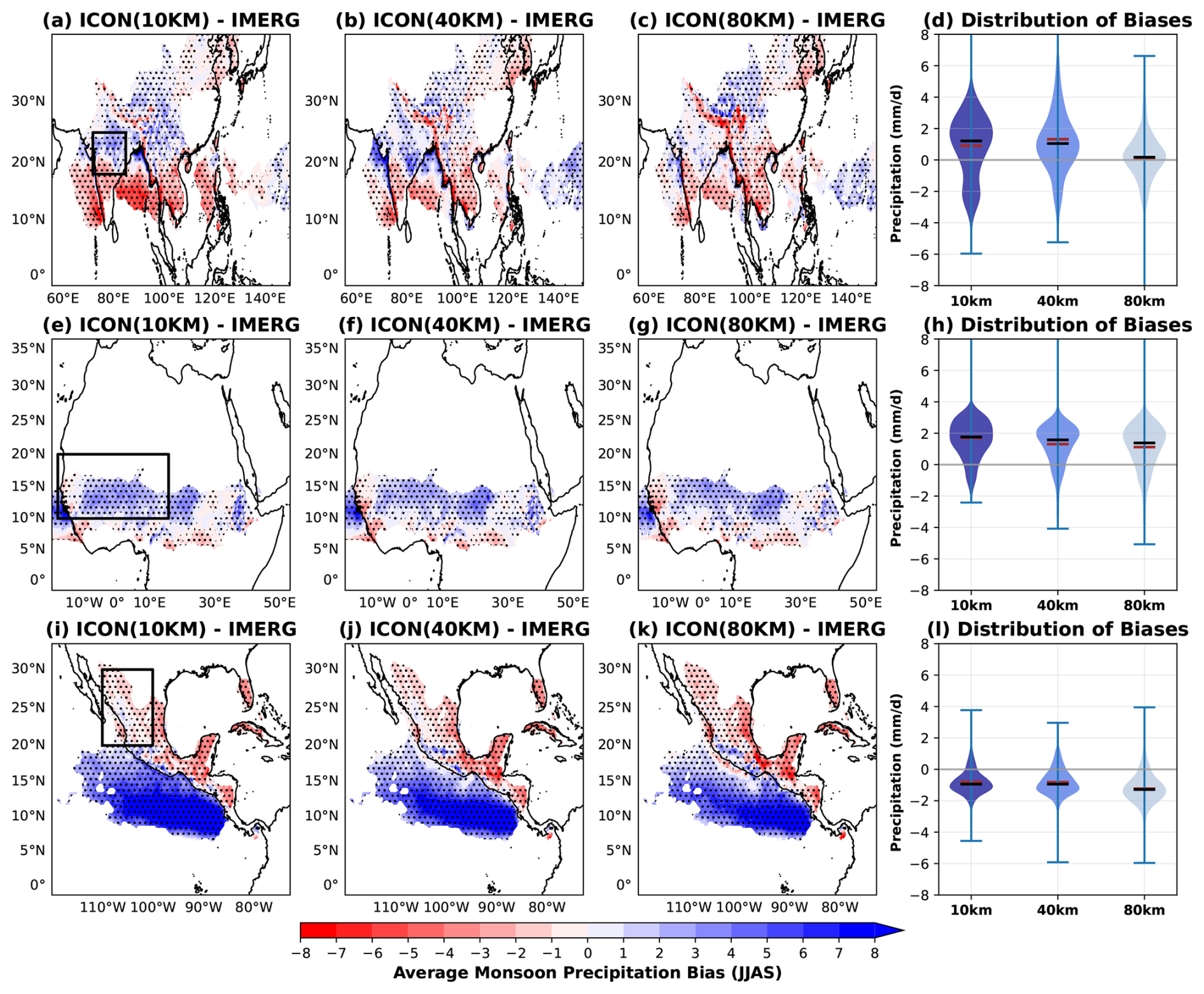
Figure 6 Spatial patterns of the mean bias in the total precipitation occurring during the summer monsoon season (JJAS) in various simulations with reference IMERG dataset over the (a–d) SAsiaM, the (e–h) WAfriM, and the (i–l) NAmerM domains respectively. Stippling indicates grid points where the bias is statistically significant at the 95 % confidence level based on a two-sided t test of log (1+P) transformed precipitation data.The black boxes in the domains indicate the respective core monsoon regions of (a) SAsiaM, (e) WAfriM and (i) NAmerM, and the violin plots show the bias distribution of total precipitation over the highlighted box regions. The black bar in the violin plots indicate the median, while the brown bar indicates the mean of the total precipitation bias.

All simulations reproduce observed precipitation patterns well, but region-specific differences remain. We quantify these biases in Fig. 6 by showing the difference between the simulations and IMERG, followed by an investigating into the monsoon core regions using violin plot. Over the SAsiaM domain (Fig. 6a–d), all runs exhibit a coherent dipole bias pattern, a systematic dry bias (> 2 mm d⁻¹) over the southern Indian peninsula and adjacent equatorial Indian Ocean coupled with a wet bias (≈ 2 mm d⁻¹) over central and northern India. Additional biases include a dry bias over the foothills of the Himalayas, and a wet bias over Tibetan Plateau. Fine grid spacing (10 km) reduces the dry bias over the Himalaya and wet bias over the Tibetan Plateau, but it amplifies the wet-dry dipole bias over the Indian sub-continent. Over the monsoon core region, a median (mean) bias over central India in 10, 40, 80 km of 0.9 (1.2), 1.3 (1.0), 0.1 (0.1) mm d⁻¹ exists respectively. A bimodal distribution of bias in 10 km run further shows that finer grid spacing enhances the dipole bias pattern over India. This points out that finer grid spacing, does not necessarily improve biases, rather it might further activate regional processes over SAsiaM domain, such as orography moisture blocking, local land-atmosphere interactions or intensification of synoptic systems (Vishnu et al., 2020).

Over the WAfriM domain (Fig. 6e–h), all runs show a wet bias (≈ 1.5 mm d⁻¹) in the continental central Sahel, Sudanian regions and coastal Atlantic, which intensifies with finer grid spacing. Over the monsoon core region, the 10, 40, and 80 km simulations show a median (mean) bias of 1.7 (1.7), 1.2 (1.6), and 1.1 (1.3) mm d⁻¹, respectively, further indicating intensification of biases. These results are also consistent with the findings in SAsiaM core region. Over the NAmerM domain, systematic slight dry bias (≈ 0.5 mm d⁻¹) is revealed in all simulations over the Sierra Madre Occidental region, and a large wet bias over the eastern Pacific ocean (> 8 mm d⁻¹). This large oceanic bias shows a deficiency in ICON in representing tropical eastern Pacific convection, air-sea interactions, or the subtropical high-pressure system that normally suppresses rainfall in this area in summers (Adams and Comrie, 1997). Finer grid spacing (10 and 40 km) shows a slight improvement in the magnitude of dry bias (0.8 mm d⁻¹) over the monsoon core region compared to 80 km (1.2 mm d⁻¹) run.

Overall, ICON reliably simulates the large-scale patterns of SAsiaM, NAfriM, and NAmerM monsoon precipitation, but it exhibits systematic regional biases. Importantly, finer grid spacing improves some features (e.g., orographic gradients) but amplifies others, such as continental wet-dry dipoles and excessive oceanic rainfall. This demonstrates that increased resolution alone does not necessarily improve performance; it can instead more vigorously activate both realistic and biased physical processes. Furthermore, our findings remain qualitatively consistent when validated against CMORPH, ERA5 and MSWEP (shown in Fig. S10)

3.3.1 Role of Low-Level Monsoon Jets in Precipitation Biases

To diagnose potential origins of precipitation biases, we analyzed low-level moisture transport in ICON simulations and compared them against ERA5 reanalysis in Fig. 7.

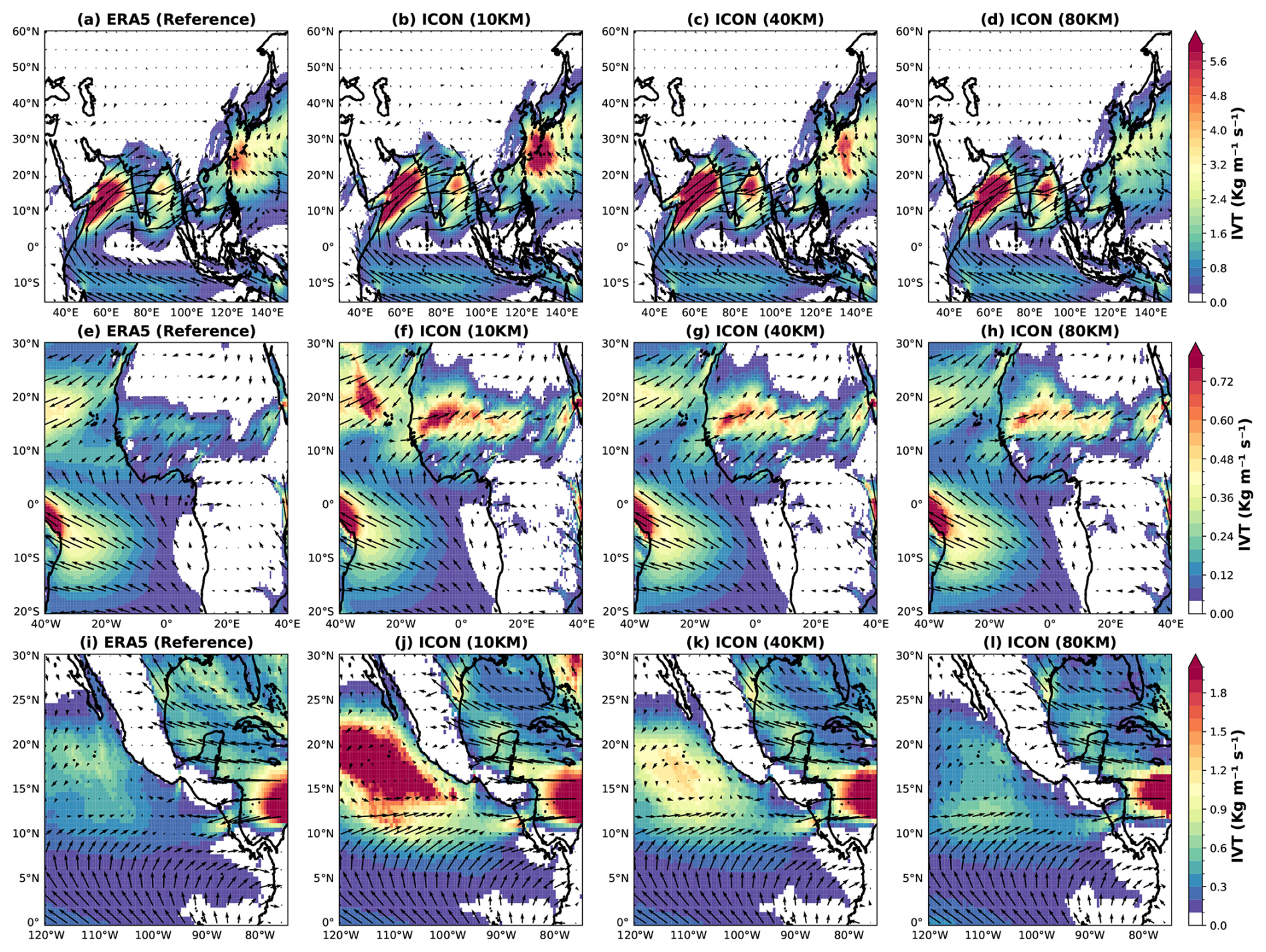
Figure 7 Spatial patterns of the vertically integrated moisture transport (IVT) near the lower boundary layer (integrated from surface to 850 hPa) during the summer monsoon season (JJAS) in reference ERA5 reanalysis dataset and various ICON simulations over the (a–d) SAsiaM domain showcasing the Findlater low level jet, the (e–h) WAfriM domain showcasing the West African Jet, and (i–l) NAmerM domain showcasing the Gulf of California Jet. All the ICON simulations are brought to a common ERA5 grid for fair comparison.

Over the SAsiaM domain (Fig. 7a–d), the ERA5 reanalysis shows the canonical cross-equatorial moisture transport from the southern hemisphere (≈ 12° S) to the northern hemisphere, which turns eastward off the Somali coast as the Findlater jet, carrying substantial moisture (> 5 kg ms⁻¹) from the western Indian Ocean towards India. A second branch of strong moisture transport is observed over the Bay of Bengal, feeding precipitation over Southeast Asia and the South China Sea, while a third hotspot over the western Pacific supplies the EAsiaM. All simulations capture the large-scale patterns of moisture transport. However, the Findlater jet moisture transport is enhanced and more oriented toward the north. While the 10 km run shows an improved pattern and magnitude over the Bay of Bengal, it unrealistically enhances moisture transport over the western Pacific off the coast of China.

For the WAfriM domain (Fig. 7e–h), ERA5 reanalysis shows a southwesterly to westerly transport of moisture from the eastern Atlantic and Gulf of Guinea towards the continent. Inland, this moist southwesterly monsoon flow meets the dry, northeasterly Harmattan winds from the Sahara, forming a sharp inter-tropical discontinuity that marks the northern boundary of the monsoonal moisture. All the simulations capture the large-scale southwesterly to westerly transport over the ocean. However, over continental Africa, specifically near the eastern/central Sahel, the Sudanian region, and the Ethiopian Highlands, all simulations exhibit a systematic enhancement of moisture flux that increases with finer grid spacing. Critically, this enhanced moisture flux reaches farther north than observed, indicating an unrealistic representation of the intertropical discontinuity. Compared to SAsiaM and WAfriM domain, the moisture flux contributing to NAmerM (Fig. 7i–l) is highly localized. The ERA5 reanalysis shows a primary moisture source over the eastern Pacific Ocean, southwest of Mexico. An important narrow branch of this flux is channeled northward towards the Gulf of California, reaching the southwest United States, while the southward flow supplies the Sierra Madre Occidental. The moisture flux is unrealistically enhanced over the eastern Pacific Ocean in fine grid simulations (10 and 40 km) compared to coarser grid simulation, indicating an unrealistic moisture convergence over open ocean. Crucially, only the 10 km simulation shows a realistic moisture flux through the Gulf of California, while at coarse grid spacing ICON struggles to capture this feature. This indicates the importance of fine grid spacing in correctly capturing the channeled low-level jet over the Gulf.

To further quantitatively evaluate the performance of ICON's low-level moisture transport and the impact of grid spacing, we show the spatial bias patterns and corresponding statistics using a violin plot in Fig. 8.

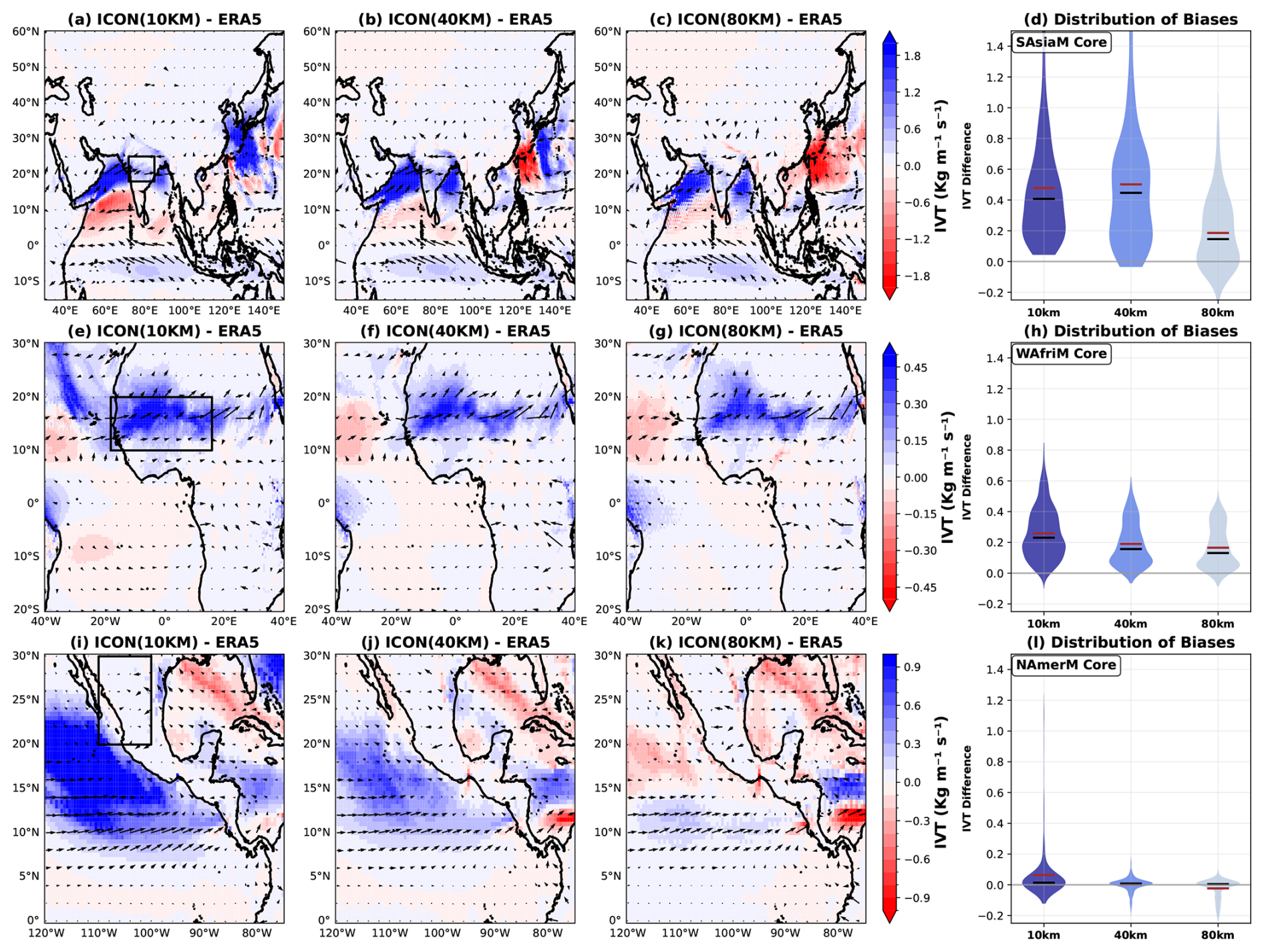
Figure 8 Spatial patterns of the mean vertically integrated moisture transport (IVT) bias near the lower troposphere during summer monsoon season (JJAS) in various ICON simulations with ERA5 reanalysis over the SAsiaM domain (a–d), WAfriM (e–h), and NAmerM domains (i–l). The black boxes in the (a) SAsiaM, (e) WAfriM and (i) NAmerM domains indicate the respective core monsoon regions, and the violin plot on the right panels show the bias distribution of IVT over the box regions. The black bar in the violin plots indicate the median, while the brown bar indicates the mean of the IVT bias distribution.

Over the SAsiaM domain (Fig. 8a–d), all simulations systematically overestimate the moisture flux over the northern Indian ocean (> 1.5 kg ms⁻¹), while slightly underestimating it in the southern Indian ocean, with 10 km simulation showing the largest southern ocean deficit (≈ 1 kg ms⁻¹). These moisture flux biases can be directly related to the north-south dipole precipitation biases (Fig. 6), where all the simulations exhibit a wet bias over northern India and a dry bias over southern India. Over the SAsiaM core region, the median (mean) moisture flux bias increases from 0.19 (0.15) kg ms⁻¹ in the 80 km run to 0.50 (0.45) and 0.48 (0.41) kg ms⁻¹ in the 40 and 10 km runs, respectively. Thus, the amplification of precipitation biases with finer grid spacing is related to these moisture flux biases. Furthermore, pronounced and unsystematic biases in the moisture flux over the western Pacific Ocean, off the coast of China, underscore ICON's deficiencies in capturing the moisture transport feeding the EAsiaM domain.

A systematic and pronounced moisture flux dominates in all ICON simulations over the continental WAfriM domain (Fig. 8e–h). The magnitude of this overestimation increases with finer grid spacing, with the 10 km run showing the largest bias (> 0.2 kg ms⁻¹), while biases over the ocean remain small. This excessive continental moisture flux explains the widespread precipitation wet bias over the Sahel, Sudanian and Ethiopian Highland regions. Additionally, a northward extent of the enhanced flux indicates a northward shift of Africa's monsoon moisture convergence zone. Over the WAfriM core region, 10 km run shows a maximum median (mean) bias of 0.26 (0.23) kg ms⁻¹, followed by 40 km run with a bias of 0.19 (0.17) kg ms⁻¹, and 0.17 (0.13) kg ms⁻¹ in 80 km run, reflecting the systematic overestimation of precipitation over these core region. Over the NAmerM (Fig. 8i–l), the moisture flux biases over the continental core region remain relatively small in all simulations compared to the SAsiaM and WAfriM core regions, while the finer grid spacing runs (10 and 40 km) show a large overestimation over the open eastern Pacific ocean. A notable grid spacing sensitivity is evident over the Gulf of California and eastern coast of Mexico, where the coarse grid (40 and 80 km runs) spacing shows an underestimation of flux, while the fine grid spacing 10 km run is closer to ERA5. The dry bias in precipitation over the Sierra Madre Occidental, and the southwestern United States in all simulations can not be completely explained by moisture transport patterns.

Overall, the precipitation biases are driven by errors in low-level moisture jets. While fine grid spacing corrects some localized features, such as the Gulf of California, it enhances large-scale moisture flux biases.

3.3.2 Daily Precipitation Intensities Distribution

Figure 9 shows the cumulative distribution (a–c) and probability of exceedance (d–f) of daily precipitation for the monsoon core regions, using IMERG and MSWEP as observational references.

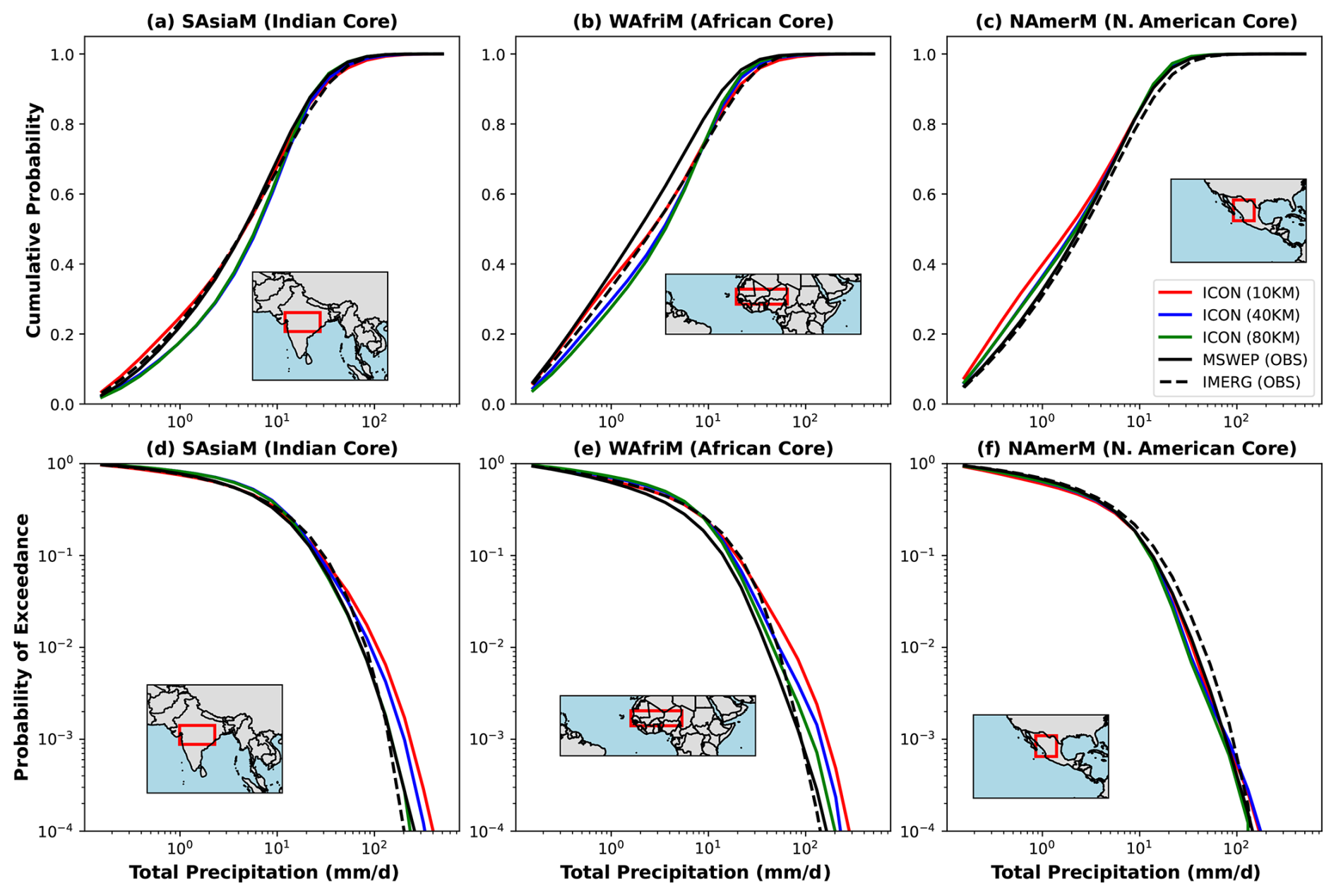
Figure 9 Cumulative probability distribution of daily total precipitation over the SAsiaM, WAfriM, and NAmerM core regions (red boxes) during local summer monsoon season (JJAS). Panels (a)–(c) show the cumulative probability distribution function on a linear probability scale, highlighting biases in light-moderate rainfall frequency. Panels (d)–(f) show the complementary cumulative distribution function, or probability of exceedance on a logarithmic probability scale to emphasize extreme precipitation. The IMERG and MSWEP observational datasets (in solid and dotted black lines respectively) are used to compare against model simulations.

Over the SAsiaM (Fig. 9a–d) core region, 10 km simulation shows excellent agreement with observations in light to medium precipitation intensities (1–10 mm d⁻¹). However, in the extreme tail, it overestimates the probability of exceedance (> 10 mm d⁻¹), indicating that its wet bias over this region is driven primarily by an excess of intense daily events. The coarser grid spacing runs underestimate the frequency of light-to-medium rain events, but diverges for extremes. The 40 km overestimates intense events, while 80 km shows better agreement with observations. Overall, finer grid spacing increases the simulated frequency of extreme daily rainfall over the SAsiaM domain.

Over the WAfriM (Fig. 9b–e) core region, 10 km shows a good agreement in light and medium precipitation events with MSWEP observational dataset. The observations, IMERG and MSWEP slightly disagree in this regime, underscoring the observational uncertainties. The coarse-grid-spacing simulations underestimate the light and medium precipitation events compared to both IMERG and MSWEP datasets. All the simulations systematically exhibit a high frequency of intense precipitation events, with 10 km simulation showing the highest overestimation followed by 40 km. This indicates a consistent enhanced convective activity in ICON over WAfriM, contributing to the wet precipitation bias in this region.

Applying the cumulative probability distributions to the convective precipitation (Fig. S11) reveals that the low and medium rain closely follow the behavior of total precipitation as in Fig. 9. However, for intense precipitation events, all the simulations show no distinct differences in convective precipitation, unlike the clear resolution dependence seen in total precipitation. This indicates that the enhanced frequency of intense total precipitation arises from the sensitivity of grid-scale (resolved) precipitation to grid spacing, while intense convective precipitation exhibits a more nuanced, resolution-invariant behavior. Consequently, the enhanced wet bias over SAsiaM and WAfriM regions at fine grid spacing is likely driven by an overproduction of precipitation by the grid-scale processes in response to better resolved dynamical forcing.

All the ICON simulations overestimate the frequency of light rain events (≈ 1–5 mm d⁻¹) over the NAmerM (Fig. 9c–f) core domain. In the intense precipitation regime (10–80 mm d⁻¹), the 10 km run shows good agreement with IMERG, though there is a slight discrepancy between IMERG and MSWEP. For extreme events (> 80 mm d⁻¹), the 10 km run produces an overestimation. The coarser resolutions exhibit different biases, both 40 and 80 km slightly underestimate intense precipitation, while the 40 km run also overestimates the extreme tail. These results underscore the greater complexity and finer scale of controlling processes in the NAmerM compared to the SAsiaM and WAfriM regions.

Furthermore, we investigated the partition of convective and grid-scale (resolved) precipitation across the simulations over monsoon core regions. Results indicate that fine grid spacing (10 km) induces more grid-scale precipitation compared to the coarse grid spacing simulations (40 and 80 km) in all three monsoon cores. Notably, over the SAsiaM, from 28 % to 46 % and NAfriM, from 12 % to 30 % in 10 to 80 km simulation respectively. Correspondingly, the convective fraction decreases. This indicates that fine grid-spacing allows the model to generate more explicitly resolved precipitation, reducing the dominance of parameterized convection. However, it is important to note that the rate of increase in the grid-scale precipitation is not proportional to the decrease in convective precipitation. For example, over South Asia, the 10 km simulation's grid-scale gain exceeds the convective loss by a factor of 1.7. This indicates that fine grid spacing does not merely partition the existing precipitation, but generates additional precipitation through explicitly resolved dynamics.

Further analysis reveals that the increase in grid-scale precipitation in fine grid spacing simulations is due to efficient microphysical processes in the lower troposphere. This is largely attributed to efficient conversion of rain content (Fig. S12) from the cloud water content in the cloud microphysics, coupled with increased vertical velocity and enhanced large-scale moisture advection into the monsoon core.

In summary, the analysis reveals that fine grid spacing systematically amplifies the simulated frequency of extreme daily precipitation, which is a primary driver of the mean wet biases over the SAsiaM and WAfriM core regions. Specifically, this amplification is attributed to an increase in resolved grid-scale precipitation relative to convective precipitation, largely driven by efficient cloud microphysics processes coupled with large-scale moisture advection. Over NAmerM, the relationship is more nuanced, reflecting the complex, fine-scale processes that govern precipitation in this region.

3.4 Monsoon Precipitation Variability at Interannual, Intraseasonal and Diurnal Scales

Here, we assess the ICON performance across various timescales to investigate the representation and sensitivity of monsoon variability to grid spacing. Figure 10 shows the spatial patterns of variance ratio (ICON/IMERG) associated with 30–90 d bandpass filtered daily precipitation data over the SAsiaM (a–d), WAfriM (e–h) and NAmerM (i–l) domains.

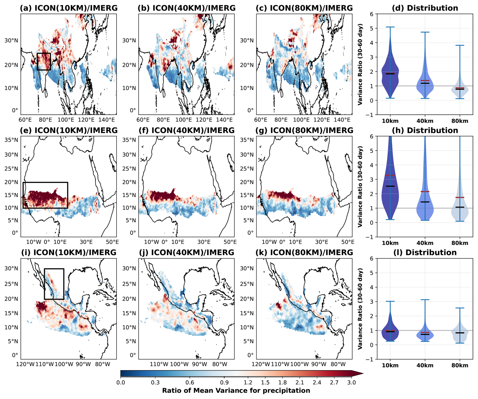
Figure 10 The Spatial patterns of 30–60 d filtered precipitation variance of ICON divided by the variance of IMERG during summer monsoon season (JJAS) representing intraseasonal variability for the (a–d) SAsiaM, the (e–h) WAfriM and the (i–l) NAmerM domains. The regions highlighted in the black box represents core monsoon region for (a) SAsiaM, (e) WAfriM, and (i) NAmerM domains. The violin plot on the right most panels show distribution of the variance ratio's in the core monsoon domains, with black bar indicating the median, while the brown bar indicates the mean of the distribution.

Over the SAsiaM domain, the 10 km simulation shows an overestimation of intraseasonal variability, with a peak variance ratio > 1.5 over the central Indian monsoon core region, Bangladesh and eastern Tibetan Plateau. The 40 km simulation also overestimates the variance over the monsoon core region, but the peak pattern is confined more towards the east coast of India. In contrast, the ICON 80 km variance ratio is ≈ 1 over most of the domain. Over the monsoon core region, the median (mean) variance ratio is 1.9 (1.8) for 10 km, 1.4 (1.1) for 40 km, and 0.8 (0.7) for 80 km simulation. This systematic resolution dependence, where the fine grid spacings produce greater intraseasonal variance, explains the earlier finding of enhanced extreme-precipitation frequency. The 10 km simulation exhibits approximately 58 % greater variance than the 80 km run. Since the 30–90 d variability in this domain is largely governed by the boreal summer intraseasonal oscillation and tropical waves, these results suggest that the simulation of these large-scale convective phenomena is highly sensitive to model grid spacing.

In the WAfriM domain, all the simulations systematically overestimate the variance, with most of the overestimation occurring in the Sahel region. The spatial patterns of this variance overestimation exhibit a clear north-south gradient, closely mirroring the mean precipitation bias shown in Fig. 6. The magnitude and the spatial extent of the overestimation increase with fine grid spacing. The 10 km simulation shows the highest variance > 2, and also covers a larger swath over the Sahel compared to the coarse grid spacing simulations. Quantitatively, over the monsoon core region, the median (mean) variance ratio is 3.2 (2.4), 2.1 (1.4), and 1.7 (1) for ICON 10, 40, and 80 km simulation, respectively. This represents an 88 % increase in mean core variance from 80 km run to 10 km, the largest resolution-induced amplification among all three monsoon domains. Over the continental NAmerM domain, the spatial patterns of variance ratio in ICON simulations look almost identical, but with a slightly enhanced variance over the Sierra Madre Occidental in 10 km simulation compared to coarser grid spacing runs. Over the monsoon core region, the median (mean) variance ratio is 1 (0.9) for 10 km, 0.9 (0.7) for 40 km, and 0.8 (0.8) for 80 km simulation. This indicates a slight underestimation of 30–90 d variability across all simulations, with minimal sensitivity to model grid spacing. These results qualitatively agree when simulations are compared to MSWEP, CMORPH and ERA5 observations (Figs. S13–S15)

Next, we investigated the 2–30 d high frequency variability (Figs. S17–S20) across the domains. The results mirror those of the 30–90 d band, i.e., the finer grid spacing systematically amplifies variance, with ICON 10 km showing the highest variance over the SAsiaM and WAfriM domains. The percentage increase over the SAsiaM core monsoon region between the ICON 10 and 80 km is ≈ 54 % and 42 % over WAfriM. In these regions, the high-frequency 2–30 d oscillations are generally attributed to synoptic systems, wave activity, which contributes to active/break monsoon periods. Often, these systems are attributed to the extreme precipitation over these regions, causing massive flooding. Key examples include low pressure systems (LPS) over of the Bay of Bengal that propagate northwestward into the Indian core region, and African Easterly Wave activity that triggers organized mesoscale convective systems over the Sahel. We investigate these processes explicitly in the following section.

In contrast, over the NAmerM domain, variance is suppressed (ratio < 1) in all the simulations, suggesting that the model does not fully resolve the key drivers of high-frequency variability in this region, such as Gulf of California moisture surges. Analysis of interannual variability (Fig. S22) shows similar resolution-dependent patterns, but we do not emphasize these results, as a simulation period longer than our 10-year sample is required for robust statistics at these longer timescales. Overall, the analysis of 30–90 and 2–30 d bands demonstrates that finer grid spacing systematically amplifies precipitation variance across the SAsiaM and WAfriM monsoons, with the strongest effect occurring at the finest resolution (ICON 10 km).

To determine if intense precipitation in fine grid spacing simulations disproportionately influence the variance ratios, we applied a log (1+P) transformation to all precipitation (P) datasets prior to band-pass filtering. This transformation reduces the statistical leverage of intense rainfall, while preserving the timing of precipitation events. After transformation, the systematic increase of variance persists across both the 30–90 and 2–30 d bands over SAsiaM and WAfriM domains (Figs. S16 and S21). Crucially, the transformed variance ratios are below unity for 2–30 d, revealing that all simulations underestimate organized precipitation variability when intense precipitation is statistically controlled, while the ratio of 30–90 d in fine grid spacing remains near unity. This indicates that the variance ratios exceeding 1 in raw data primarily reflect the fine-grid simulations over production of intense precipitation (> 10 mm d⁻¹). These findings are robust when seasonal cycle is removed in both raw and transformed datasets. The persistence of grid spacing dependence on variance ratios after transformation confirms they represent real model sensitivities rather than statistical artifacts from intense precipitation.

Finally in Fig. 11, we examine the spatial patterns of the local hour of maximum precipitation (peak diurnal timing) in local solar time (LST) compared against IMERG during the local summer monsoon season.

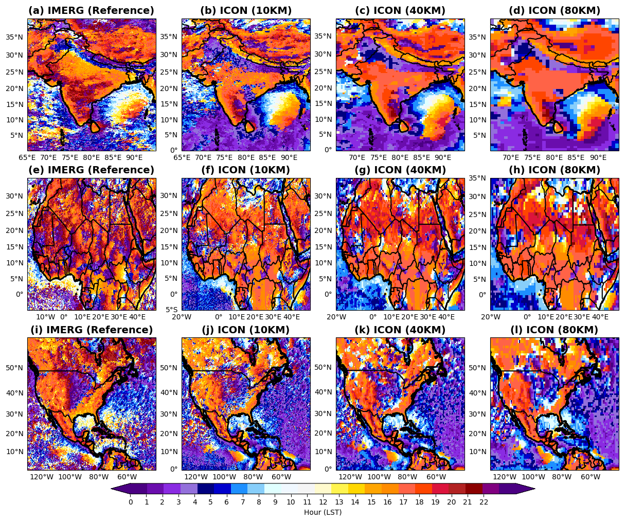
Figure 11 The local solar time (LST) at which maximum precipitation occurs on average during the summer monsoon season (JJAS), showcasing a peak time of diurnal cycle in IMERG reference dataset and the ICON simulations over the (a–d) SAsiaM, (e–h) WAfriM, and (i–l) NAmerM domain. The shading of blue/dark purple indicates a nocturnal maxima while the colors shaded from yellow/red show afternoon or late evening peak.

Over the SAsiaM domain Fig. 11a–d, IMERG shows a wide spread afternoon peak (≈ 15:00–18:00 LST) over continental India, and the Tibetan Plateau, driven by strong daytime land-surface heating, and a nocturnal peak over the adjacent oceans, likely associated with nighttime cloud-top cooling and local air–sea interactions (Fang and Du, 2022). Notable exceptions include a nocturnal peak over the Himalayas and its adjacent foothills associated with the interaction of katabatic winds with the monsoonal flow, and a patchy nocturnal to afternoon transitions over the open oceans. All simulations capture the diurnal signal over the continental afternoon/oceanic nocturnal signal. However, ICON 10 km marginally better agrees in the timing of the peak signal (≈ 15:00–18:00 LST), while 40 and 80 km simulations exhibit slight delay, with a peak occurring mostly at ≈ 18:00 LST. All simulations are unable to reproduce the nocturnal peak over the Himalayas, instead they unrealistically produce the peak towards the south of the Himalayan foothills. Over the oceans, the simulated diurnal phase patterns align well with observations across all grid spacings.

Over the continental WAfriM domain Fig. 11e–h, IMERG shows a wide spread late afternoon maxima (≈ 16:00–18:00 LST) over the interior, primarily driven by land surface heating, and a coastal zone with nocturnal maxima along the Guinea coast, eastern Atlantic and coastal Sahel indicative of land-sea breeze convergence. Inland nocturnal patches are observed, particularly over the central Sahel, likely associated with the propagation of mesoscale convective systems initiated during the afternoon. All the simulations capture the broad inland afternoon peak. The 10 km simulation marginally better reproduces the timing, while the coarse grid spacing show a slight delay. The coastal early morning peak near the Sahelian coast is also well captured in all the simulations, indicating that the local land-sea breeze is reasonably well simulated.

Over the NAmerM domain Fig. 11i–l, IMERG reveals the expected afternoon maximum (≈ 15:00–18:00 LST) over the orographically complex regions of western North America (Sierra Madre Occidental, Rocky Mountains) and Central America, driven by slope heating, as well as over the eastern US and coastal regions, driven by land-surface heating. A distinct early morning peak (≈ 03:00–07:00 LST) over the Great plains resulting from the nocturnal eastward propagation of mesoscale convective systems initiated over the mountains. A nocturnal peak dominates open oceans, while patchy afternoon peaks are observed near coast lines. All simulation capture the broad pattern of afternoon peak over both, the eastern and western North American regions. The 10 km simulation shows the correct peak time, while the coarser grid spacing runs exhibit a slight delay, consistent with the behavior seen over SAsiaM and WAfriM continents. The nocturnal maximum over the central plains of America is also simulated well in all simulations. Overall, the diurnal phase is surprisingly well simulated in all the simulations, with 10 km run providing only marginal improvement in timing over land.

These results demonstrate that while finer grid spacing improves some aspects of monsoon simulation (diurnal timing, variance structure) depending upon the region, it exacerbates others (extreme overproduction, mean biases), revealing complex trade-offs in fine grid spacing monsoon modeling.

3.5 Processes Associated with SAsiaM and WAfriM Domain's High Frequency Intraseasonal Variability (2–30 band)

The previous section analysis showed that ICON's fine grid spacing systematically amplified the variance in the 2–30 d band over the SAsiaM and WAfriM domains. Here we investigate the characteristics of the processes responsible for this variability, namely the rain carrying synoptic low pressure systems over SAsiaM domain and African Easterly wave activity. While the 30–90 d mode shows similar behavioral trends, its dynamics involve more complex large scale ocean–atmosphere interactions that extend beyond the scope of this regional process evaluation.

Low pressure Systems and African Easterly Waves

Figure 12 shows the detected track of low pressure systems, depressions, deep depressions, cyclonic storms and severe cyclonic storms in (a) IMD observations, (b) ERA5 reanalysis, and various (c–e) ICON simulations. The LPS systems in IMD and ERA5 show the classical northwestward propagation from the Bay of Bengal into the continental land mass. These systems typically make landfall between ≈ 15 to 25° N, impacting a wide swath of the Indian subcontinent. They extensively contribute to the synoptic variability (2–30 d band) and are often triggered under the influence of ITCZ near the head of Bay of Bengal (Saha et al., 2019). Methodological differences in identification lead to discrepancies in the track intensities (shown in track color) between the IMD and ERA5. The IMD uses a subjective best track estimates based on a series of observational network, while the ERA5 tracks are obtained by applying our in-house objective tracking algorithm.

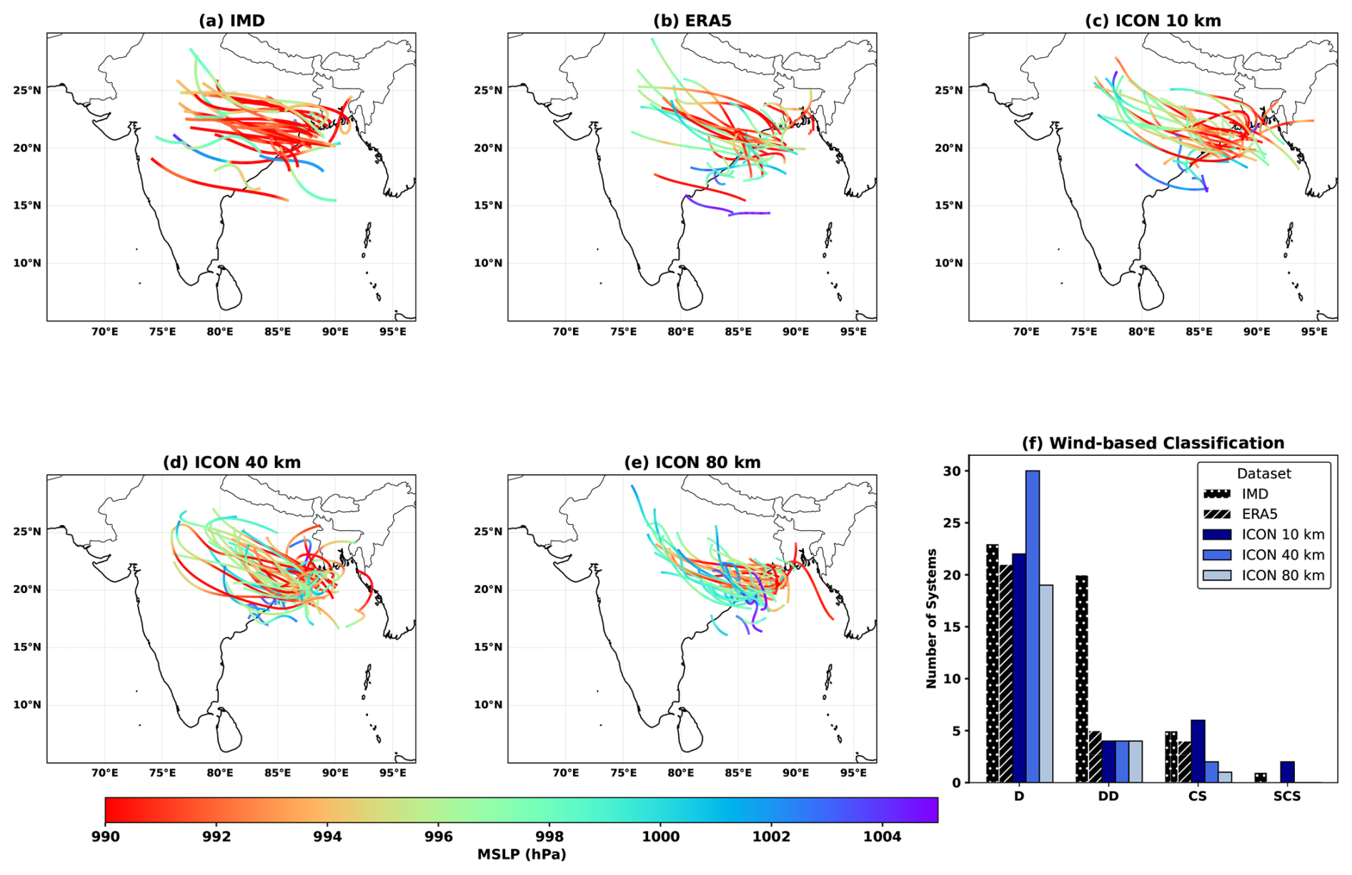
Figure 12 Best track estimates based on minimum surface pressure and 850 hPa stream function around the local minima of all the north-westward propagating low pressure systems during the JJAS season over the SAsiaM domain. The (a) IMD best track estimates are based on subjective analysis, while the (b) ERA5 and various (c–e) ICON simulations used a common tracker. The colors of the tracks indicate the minimum surface pressure during the north-westward propagation, while the (f) bar plots show the number of detected systems based on the classification of LPS systems (depressions (D), deep depressions (DD), cyclonic (CS) and sever cyclonic storms (SCS)) by the IMD.

All the simulations reproduce the northwestward movement of the LPS. However, the 80 km run shows an unrealistic, narrow concentration of tracks near the head Bay of Bengal compared to IMD and ERA5. Further wind based classification reveals that the 10 km run overestimates the frequency of cyclonic storms and severe cyclonic storms, while the 40 km overestimates the frequency of depressions. The coarse 80 km simulation underestimates the frequency of intense LPS systems. Thus, the greater 2–30 d variance in the finer-grid spacing runs can be partially attributed to this overestimation of intense LPS activity (Fig. 12f). Our results remain consistent when the analysis is conducted on the original grid spacing of the simulations and ERA5 reanalysis data indicating robustness.

Figure 13 shows the vertical profile of the zonal winds averaged over the longitudes 10° W–10° E, highlighting the representation of the African Easterly Jet, Tropical Easterly Jet, and low level moist westerly flow in (a) ERA5 and our (b–d) simulations. The ERA5 profile shows two prominent jets, the TEJ (between the red vertical lines, ≈ 400–100 hPa, 5° S–10° N) and the AEJ (between the black vertical lines, ≈ 700–500 hPa, 10–20° N), along with a weaker low-level westerly flow. Additionally a less intense moist westerly low level flow is also seen over the African continent. All the simulations realistically capture the location and strength of the AEJ (> 6 m s⁻¹), however they consistently exhibit strong westerly moist flow, consistent with the moisture transport and precipitation biases shown in Figs. 6 and 8. The location of the TEJ is slightly displaced towards the south of Guinea Coast (near 5° S), and its magnitude intensified in all simulations. The realistic representation of the AEJ is crucial, as it governs the organization and steering of rain producing mesoscale convective systems. While previous studies attributed mean precipitation bias over WAfriM with the location and strength of easterly jets, in ICON the dominant bias appears to originate from an overly intense low-level westerly moisture flux.

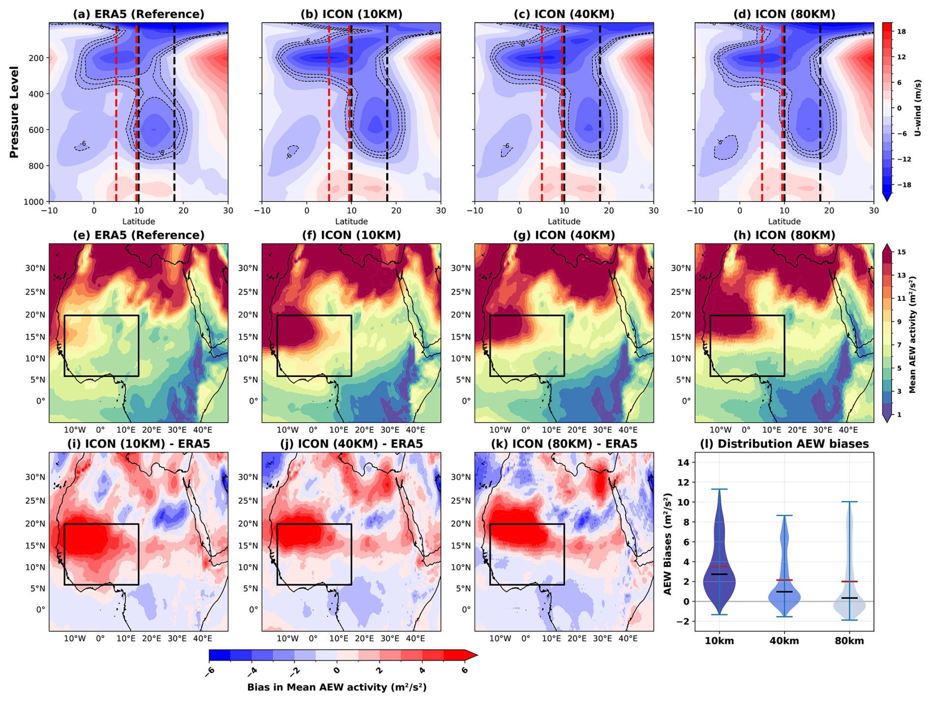
Figure 13 The top panel shows the vertical cross section of the zonal winds (m s⁻¹) averaged over the longitudes 10° E–10° W indicating the location of African Easterly Jet (contours > 6 m s⁻¹ indicating the AEJ region) in (a) ERA5 reference and various (b–d) ICON simulations. The black dotted vertical lines indicate the approximate location of the Sahel and the red lines indicate Guinea coast. The middle panel shows the 2–10 d bandpass filtered variance of the meridional wind over the African continent indicating the African Easterly Wave (AEW) activity in (e) ERA5 and various (f–h) ICON simulations with the black box indicating the core monsoon AEW activity. Panels (i)–(k) shows the difference in AEW activity between various ICON simulations against ERA5 reference, and the (f) violin plot shows the AEW bias in the core region with black horizontal line indicating the median and the brown line indicating the mean.

Figure 13e–h shows the high frequency variance associated of meridional velocity, representing the African Easterly Wave activity driven by the barotropic and baroclinic instabilities of the AEJ. The ERA5 shows a variance of ≈ 5–9 m² s⁻² over the central Sahelian region (black box), increasing gradually towards its coast. All the simulations systematically overestimate the AEW activity across the Sahel as confirmed by the Fig. 13i–k bias panels. Quantitatively, the mean (median) value of AEW variance is 2.7 (3.5) m² s⁻² for 10 km, 0.9 (2) m² s⁻² for 40 km and 0.3 (2) m² s⁻² for 80 km. This systematic amplification of AEW activity with finer grid spacing provides a direct dynamical explanation for the enhanced 2–30 d precipitation variance over the WAfriM core region.

In summary, the enhanced sub-seasonal variance in the fine grid spacing simulations is consistent with an overestimation of key synoptic drivers, namely the low pressure systems over the SAsiaM and the African Easterly Wave activity over the WAfriM domain. Furthermore, these processes are also potentially responsible for the increase in extreme precipitation frequency and mean wet biases in these regions. This demonstrates that finer grid spacing not only enhances variance statistically, but also intensifies the representation of the physical systems that contribute to the monsoon precipitation variability.

4 Summary and Conclusion

This study provides a comprehensive evaluation of global and northern hemispheric regional monsoon systems simulated by the ICON model across three horizontal grid spacings (10, 40, and 80 km), with a focus on the effects of grid spacing.

Applying the objective global monsoon definition of (Wang and Ding, 2008), we demonstrate that ICON robustly captures the large-scale spatial structure of the global monsoon domain and its regional sub-domains. These include the North American (NAmerM), South American (SAmerM), West African (WAfriM), South and South East Asian (SAsiaM), East Asian (EAsiaM), Australian-Maritime Continent (AusMCM), and the South African Monsoon (SAfriM) systems that are well established in the literature (Masson-Delmotte et al., 2021). All the runs exhibit significant skill in delineating these domains, with annual range spatial correlations exceeding 0.7 against an ensemble of observations, and a domain detection accuracy of above 80 %. Notably, the 10 km simulation exhibits a greater root mean square error of annual precipitation range compared to its coarser counterparts by ≈ 15 %–17 %, a discrepancy originating largely over oceans. This indicates that the fine grid spacing amplifies precipitation biases in oceanic regions, even as it maintains the high skill (accuracy > 80 %) in capturing the spatial monsoon domains over land and ocean.

Assessing the monsoon onset, a fundamental characteristic, we find that all the simulations generally capture the observed large scale propagation patterns, the southeast to northwest propagation over SAsiaM, northward propagation over WAfriM, and the delayed onset (June–July) over the core NAmerM. The dependency of the onset timing to the grid spacing is regionally dependent. It shows a non-systematic (non-monotonic) dependence over SAsiM and NAmerM, but a systematic improvement with fine grid spacing over WAfriM. This demonstrates that grid spacing alone universally can not correct the onset biases, model performance is governed by a complex interplay of local to regional processes whose sensitivity to grid spacing varies across monsoon domains.

The model simulations generally captured key total precipitation spatial features over the SAsiaM, WAfriM and NAmerM, but few region specific biases such as a bi-polar north-south wet-dry bias over SAsiaM, wet bias over WAfriM and, dry bias over NAmerM core persists independent of grid spacing. The fine grid spacing further increased the biases over SAsiaM, WAfriM, but a slight improvement in dry bias over NAmerM region. The precipitation cumulative distributions show a pronounced overestimation in the frequency of intense daily total precipitation (> 10 mm d⁻¹), with a large contribution from resolved grid-scale precipitation, contributing to the enhancement of mean and extreme precipitation bias. Furthermore, we find that the enhanced grid-scale precipitation is largely due to the efficient microphysical processes (conversion of cloud water to warm rain), a process dominated by increased vertical velocity. Notably, the increment in the contribution of grid-scale precipitation with fine grid spacing is by a factor > 1.5 times the convective precipitation. This points out for a necessary implementation of scale aware convective physical parametrization in ICON (Wang, 2022; Park et al., 2024).

This intensification is also dynamically rooted in errors of low-level moisture transport. The precipitation biases over SAsiaM and WAfriM are largely attributable to discrepancies in the magnitude and location of key monsoonal jets (e.g., the Somali Jet and the West African westerly flow), which are systematically enhanced at higher resolution. Thus, the model's overactive large-scale circulation, when combined with finer grid spacing, disproportionately amplifies moisture convergence in already-biased regions.

The precipitation variability at intraseasonal timescales over SAsiaM, WAfriM domains show large sensitivity to grid spacing, while the signal is more nuanced over NAmerM domain. Specifically, the variance associated with 30–90 and 2–30 d band over the core monsoon regions systematically increased with fine grid spacing in 10 km simulation compared to the 80 km, stemming largely from the sensitivity to intense precipitation events in the fine grid spacing simulations. Supporting this, a sensitivity analysis using log-transformed precipitation, which reduces the statistical influence of extremes confirms the resolution dependence is real and not an artifact. However, when intense rainfall is statistically controlled, the models underestimate organized synoptic variability, highlighting a dual bias: an overestimation of intense precipitation coupled with an underestimation of moderate organized rainfall. In contrast, the diurnal cycle of precipitation is surprisingly well simulated across all simulations, with ICON capturing the observed peak timing patterns across all three domains. The primary added value of fine grid spacing here is a marginal correction of the delayed continental peak evident in the coarser runs. This dichotomy indicates that while local, thermally forced processes like the diurnal cycle can be directly improved by finer grids, the simulation of larger-scale organized convective variability (intraseasonal oscillations) is more complex and can be disproportionately amplified.

Process-based analysis of the systems dominating the 2–30 d band confirms that the amplified variance at finer grid spacing is dynamically rooted in an intensification of key synoptic drivers. Over SAsiaM, fine grid spacing generates more intense low-pressure systems, while over WAfriM, it enhances African Easterly Wave activity. This demonstrates that the model's representation of the fundamental processes governing monsoon variability is inherently sensitive to grid spacing, providing a dynamical confirmation of enhanced statistical variance.

In summary, this study demonstrates that the added value of fine grid spacing is not linear or universal across monsoon regions, but is strongly modulated by regional dynamics. Furthermore, finer grid spacing can amplify existing systematic biases in both the mean state and variability, indicating that it intensifies the representation of both realistic and erroneous physical processes. These conclusions are specific to the parameterized convection regime explored here (10–80 km grid spacings). A critical next step is to extend this analysis to convection-permitting kilometer scale global simulations (Dipankar et al., 2026; Prein et al., 2026), where explicit deep convection may fundamentally alter the sensitivity of monsoon systems to grid refinement.

Appendix A: Description of observational datasets used in this study

Here we describe in detail the various strengths and weaknesses of observational datasets used in this study as given in Table 1:

• IMERG combines passive microwave estimates from multiple low-earth-orbital satellites with geostationary infrared (IR) observations and gauge data. Sophisticated techniques such as morphing and Kalman filter compensate for the limited low earth orbital sampling, enabling high-temporal (30 min) and spatial resolution. However, this dataset is limited due to its indirect estimation of the infrared channel for filling temporal gaps, and morphing techniques assume linear motion. Furthermore, gauge bias correction at monthly intervals is limited over the ocean, thus enhancing the probability for bias. Despite these limitations, IMERG represents the state-of-the-art in multi-satellite precipitation estimation over the tropics.

• MSWEP uses a multitude of gauges (76 747 stations), satellites (CMORPH, GSMaP, TMPA), and reanalyses (ERA-Interim, JRA-55) to produce a global 0.1°, 3-hourly product. It has comprehensive land-ocean coverage with discharge-based bias correction (13 762 stations) and improved performance in mountains. However, its 3-hourly temporal frequency misses sub-daily extremes, its reliance on gauge stations limits performance in regions with sparse networks, discharge correction is indirect, and the complex methodology involves assumptions.

• CMORPH, similar to GPM IMERG, retrieves precipitation from passive microwave sensors deployed on low-earth orbiting satellites, and uses cloud motion vectors from geo-stationary satellites to morph precipitation. The data is also a bias-corrected version against CPC gauges (land) and GPCC (ocean). CMORPH has high temporal resolution, global coverage, and has a good warm-season performance. However, like GMPM, it uses morphing and thus assumes linear motion, has biases in complex terrain, underestimates heavy rain, and has variable regional performance.

• GPCC provides gridded gauge-based precipitation analyses derived from quality-controlled in-situ station data over global land surfaces based on up to 84 800 stations. This product uses a large station network across the globe and has established quality control procedures (Becker et al., 2013; Schamm et al., 2014). However, it is limited by variable station density and bias correction for systematic gauge measuring errors.

• CPC provides gauge-based analysis of global daily precipitation over land surfaces. It uses optimal interpolation to combine data from over 30 000 rain gauges. It uses a relatively large station network, rigorous quality control, provides estimations of gauge counts per grid cell, and accounts for orographic effects during interpolation. Like GPCC, this dataset is also limited by variable station density and has coarse spatial resolution.

• In addition to observational datasets, we used ERA5, which assimilates a vast amount of historical observations (from satellites, radiosondes, aircraft, weather stations, and ships) with a numerical weather prediction model using data assimilation to create a physically consistent, globally complete dataset.

• To validate our low-pressure system tracks from ICON, we used IMD best track datasets to estimate cyclone positions at 6-hourly intervals. It uses a multi-satellite approach for locating storm centers, including Indian geostationary satellites (Kalpana-1, INSAT-3A, and later INSAT-3D) along with polar-orbiting satellites from international partners. However, this dataset relies completely on satellites, and hence the estimates are biased, especially during periods of intense cloud cover.