the Creative Commons Attribution 4.0 License.
the Creative Commons Attribution 4.0 License.
 | 11 Aug 2020
The role of North Atlantic–European weather regimes in the surface impact of sudden stratospheric warming events
Daniela I. V. Domeisen
Christian M. Grams
Lukas Papritz
Sudden stratospheric warming (SSW) events can significantly impact tropospheric weather for a period of several weeks, in particular in the North Atlantic–European (NAE) region. While the stratospheric forcing often projects onto the North Atlantic Oscillation (NAO), the tropospheric response to SSW events, if any, is highly variable, and what determines the existence, location, timing, and strength of the downward impact remains an open question. We here explore how the variable tropospheric response to SSW events in the NAE region can be characterized in terms of a refined set of seven weather regimes and if the tropospheric flow in the North Atlantic region around the onset of SSW events is an indicator of the subsequent downward impact. The weather regime analysis reveals the Greenland blocking (GL) and Atlantic trough (AT) regimes as the most frequent large-scale patterns in the weeks following an SSW. While the GL regime is dominated by high pressure over Greenland, AT is dominated by a southeastward-shifted storm track in the North Atlantic. The flow evolution associated with GL and the associated cold conditions over Europe in the weeks following an SSW occur most frequently if a blocking situation over western Europe and the North Sea (European blocking) prevailed around the SSW onset. In contrast, an AT regime associated with mild conditions over Europe is more likely following the SSW event if GL occurs already around SSW onset. For the remaining tropospheric flow regimes during SSW onset we cannot identify a dominant flow evolution. Although it remains unclear what causes these relationships, the results suggest that specific tropospheric states in the days around the onset of the SSW are an indicator of the subsequent tropospheric flow evolution in the aftermath of an SSW, which could provide crucial guidance for subseasonal prediction.
- Article
(9701 KB) - Full-text XML
- BibTeX
- EndNote


Sudden stratospheric warming (SSW) events can have a significant impact on the tropospheric large-scale circulation and hence on surface weather (Baldwin and Dunkerton, 2001). While a causal downward link from the stratosphere after SSW events has been confirmed in idealized experiments (e.g., Gerber et al., 2009), a robust quantification of the downward impact of SSWs in observational data remains challenging. First of all, the number of SSWs in the record of satellite-era reanalysis is small (26 events from 1979 to 2019), while the case-to-case variability in terms of their tropospheric impact is large. Second, the internal variability of the troposphere itself is high, such that it can mask a stratospheric influence. Predicting if, when, and where a downward impact from SSW events will occur is therefore not straightforward, yet a better prediction of the type and timing of a downward impact would significantly benefit a wide range of users.
The tropospheric impact of SSW events is communicated by a range of mechanisms including synoptic- and planetary-scale waves (e.g., Song and Robinson, 2004; Domeisen et al., 2013; Hitchcock and Simpson, 2014; Smith and Scott, 2016). The subsequent tropospheric variability in the North Atlantic–European (NAE) region is often characterized in terms of the bimodal North Atlantic Oscillation (NAO), commonly defined through a station-based index (Cropper et al., 2015; Domeisen et al., 2018), or by the first empirical orthogonal function (EOF) of geopotential height in the North Atlantic sector. Furthermore, multimodal weather regime classifications based on k-means clustering of the leading EOFs in the North Atlantic sector tend to denote two out of several weather regimes as the positive (NAO+) and negative (NAO−) phases of the NAO given the similarity of their spatial patterns to the bimodal NAO definition (Michelangeli et al., 1995; Cassou, 2008; Ferranti et al., 2015; Charlton-Perez et al., 2018). After SSW events the NAE region tends to exhibit more persistent states of the negative phase of the NAO (Domeisen, 2019), as well as more frequent transitions towards NAO− and fewer away from NAO− (Charlton-Perez et al., 2018). NAO− is associated with enhanced meridional air mass exchanges, in particular, more cold air outbreaks in northern Europe but fewer over the Nordic Seas (Kolstad et al., 2010; Kretschmer et al., 2018b; Papritz and Grams, 2018; Huang and Tian, 2019), as well as increased precipitation in southern Europe (Butler et al., 2017; Ayarzagüena et al., 2018). The Pacific sector tends to be less strongly affected in the aftermath of SSW events (Greatbatch et al., 2012; Butler et al., 2017), though the occurrence of wave reflection in the stratosphere can be associated with Pacific blocking (Kodera et al., 2016) and cold spells over North America (Kretschmer et al., 2018a; Matthias and Kretschmer, 2020). Given the preferred occurrence and the increased persistence of certain surface signatures in the NAE region after SSW events as compared to climatology, medium- to long-range predictability over Europe has been suggested to increase after SSW events (Sigmond et al., 2013; Domeisen et al., 2015; Karpechko, 2015; Butler et al., 2016; Scaife et al., 2016; Jia et al., 2017; Beerli et al., 2017; Butler et al., 2019; Domeisen et al., 2020a). SSW events themselves are often not predictable beyond a few days to weeks, with high interevent variability (Taguchi, 2014, 2016; Domeisen et al., 2020b), although probabilistic predictability can be found for longer timescales (Scaife et al., 2016).
The analysis of the high case-by-case variability in the tropospheric signature after an SSW event is further complicated by the fact that there exists a range of different metrics for characterizing the downward impact, with each definition yielding a different set and number of SSW events with apparent surface impacts. In particular, the occurrence and type of downward impact has been investigated with respect to the SSW geometry, i.e., split versus displacement events (Charlton and Polvani, 2007; Mitchell et al., 2013; Maycock and Hitchcock, 2015; Seviour et al., 2016; Lehtonen and Karpechko, 2016), though no statistically robust differences with respect to wave geometry emerge in the tropospheric response. In addition, it has been suggested that precursors to SSW events with a downward influence differ from SSWs without such a tropospheric impact in terms of strength and location (Nakagawa and Yamazaki, 2006; Domeisen, 2019; Zhang et al., 2019), in particular with respect to forcing over Eurasia (White et al., 2019; Tyrrell et al., 2019; Peings, 2019). Furthermore, the evolution of the stratosphere–troposphere system following the SSW (Kodera et al., 2016) and in particular the persistence of the lower stratospheric response after the SSW event (Hitchcock et al., 2013a; Karpechko et al., 2017; Runde et al., 2016; Polichtchouk et al., 2018) have been found to determine the existence and type of a downward response. These studies use indices for the downward effect that are based on exclusively stratospheric or a combination of stratospheric and tropospheric indicators. For comparison, in this study we will investigate purely tropospheric indicators of the downward impact of SSW events. Definitions of a downward impact using tropospheric indicators are generally based on large-scale circulation indices such as the NAO (Charlton-Perez et al., 2018; Domeisen, 2019) or tropospheric jet location (Garfinkel et al., 2013; Afargan-Gerstman and Domeisen, 2020; Maycock et al., 2020).
Furthermore, remote forcing can affect both the stratosphere and the troposphere and thereby either mask or strengthen the downward response from the stratosphere. A range of tropical remote connections can impact the NAE region through both a tropospheric and a stratospheric pathway (Attard et al., 2019), such as the Quasi-Biennial Oscillation (QBO) (Gray et al., 2018; Andrews et al., 2019), the Madden–Julian Oscillation (MJO) (Garfinkel et al., 2014; Barnes et al., 2019), and El Niño–Southern Oscillation (ENSO) (Jiménez-Esteve and Domeisen, 2018; Domeisen et al., 2019), in addition to extratropical tropospheric forcing in the North Pacific (Honda and Nakamura, 2001; Sun and Tan, 2013; Drouard et al., 2013), Arctic sea ice (Sun et al., 2015), and snow cover in Eurasia (Cohen et al., 2014). It therefore has to be kept in mind that the stratosphere is only one possible forcing of the troposphere.
Given the large variability of the tropospheric flow evolution following SSW events and the influence of additional remote factors mentioned above, the prediction of the SSW response in the troposphere remains difficult for an individual event, despite the general shift towards NAO negative conditions in a statistical sense. The goal of this study is to investigate if tropospheric flow regimes in the NAE region can help us understand the variability of the SSW response in the observational record. More specifically, we here address the question of whether the tropospheric flow evolution in the NAE region after an SSW is statistically different from that without an SSW using seven weather regimes in the NAE region. Weather regimes are quasi-stationary, recurrent, and persistent patterns of the large-scale extratropical circulation (e.g., Michelangeli et al., 1995). While many studies showed that there are preferred transitions between different regimes, internal tropospheric variability is high and a regime onset often occurs on short timescales (e.g., Vautard, 1990; Michel and Rivière, 2011). Therefore predictability due to regimes arises from regime persistence on timescales of several days rather than typical regime sequences over several weeks. However, recent work revealed important shifts of regime occurrence and transition probabilities between regimes on subseasonal timescales of several weeks depending on the external forcing such as the stratospheric polar vortex state (Charlton-Perez et al., 2018; Papritz and Grams, 2018; Beerli and Grams, 2019). This motivates the study at hand aiming at investigating if the variability in the tropospheric flow evolution following SSW events can be characterized in terms of the weather regime around the SSW onset.
2.1 Data and classifications
ERA-Interim reanalysis (Dee et al., 2011) from 1979 to 2019 is the data basis for this study. The SSW events are defined based on daily mean data at the native ERA-Interim horizontal grid resolution. The SSW central dates are defined as the first day of easterly zonal mean zonal winds at 10 hPa and 60∘ N between the 1 December and 31 March. Events have to be preceded by at least 20 consecutive days of daily mean westerly winds. If an event fulfills the criterion for both a SSW and a final warming event, it is excluded from the analysis. Final warming events are defined as the first day of the year when the zonal mean zonal winds at 10 hPa and 60∘ N reverse and do not return to westerly for more than 10 consecutive days. These SSW central dates agree with Table 2 in Butler et al. (2017), which provides central dates up to 2013, and are defined using the same criterion thereafter. The central dates for the more recent SSW events are 12 February 2018 and 2 January 2019 (see Table 1). Following Karpechko et al. (2017) the event on 24 March 2010 has been excluded to avoid an overlap with the aftermath of the SSW event on 9 February 2010. This yields 25 SSW events for the period 1979–2019.
The tropospheric flow over the NAE region is described in terms of seven year-round weather regimes defined in Grams et al. (2017) based on 6-hourly data for the period 1979–2019 using 1.0∘ horizontal resolution (Appendix Fig. A1). As for the canonical seasonal definition using four regimes (e.g., Michelangeli et al., 1995; Michel and Rivière, 2011; Ferranti et al., 2015; Charlton-Perez et al., 2018), the mean patterns of the seven regimes are based on a k-means clustering in the phase space spanned by the leading seven EOFs (explaining 76 % of the variance) of 10 d low-pass-filtered 500 hPa geopotential height anomalies. In addition, we employ a normalized projection (weather regime index IWR) following Michel and Rivière (2011) for each of the seven regimes to define objective and persistent weather regime life cycles and for a filtering of time steps without a clear regime structure (“no regime” category). In essence, an active life cycle requires an IWR above a certain threshold for at least 5 consecutive days (minimum persistence of an active regime life cycle) and a continuous increase/decrease during the onset/decay phases (see methods of Grams et al., 2017, for details). As different life cycles can be active simultaneously, in particular during the onset and decay phases, individual days are attributed to a specific regime life cycle only if IWR is also the maximum of all IWR. The life cycle definition allows for a continuous extension of the weather regime attribution to more recent data without repeating the EOF analysis and clustering (here done for the years 2016–2019).
We use this weather regime classification to stratify SSW events according to the large-scale tropospheric flow conditions in the North Atlantic around their onset (see Table 1). To do so, we select for each SSW the dominant weather regime that is active during at least one 6-hourly time step in a time window ±5 d around the onset day (at 00:00 UTC) of the SSW. We consider a weather regime to be dominant if the mean IWR in the time window ±5 d around the onset reaches a maximum compared to other active regime life cycles. Manual inspection of the 25 considered SSW events confirms the unambiguity of this approach. An identified weather regime is required to be dominant for a minimum of 3 d in the considered 10 d period around the SSW central date.
Three of the seven regimes are dominated by a cyclonic 500 hPa geopotential height anomaly (“cyclonic regimes”; see Fig. A1a–c): the Atlantic trough (AT) regime with cyclonic activity shifted towards western Europe, the zonal regime (ZO), and the Scandinavian trough (ScTr) regime. The remaining four regimes are dominated by a positive geopotential height anomaly and are referred to as “blocked regimes” (Fig. A1d–g): Atlantic ridge (AR), European blocking (EuBL), Scandinavian blocking (ScBL), and Greenland blocking (GL).
A potential modulation of the frequency of occurrence of the seven regimes can be understood in terms of the link between the respective regimes and the NAO (Beerli and Grams, 2019, their Figs. 2 and 6). While ZO and ScTr project onto NAO+, GL strongly projects onto NAO−. EuBL and AT do not project strongly onto either NAO phase.
2.2 Statistical testing
Since SSW events only occur roughly every second winter (Butler et al., 2017), the subsequent stratification according to tropospheric flow conditions requires careful statistical testing to extract significant results that are distinct from sampling uncertainty. The overarching questions we address in this study are whether after SSWs the tropospheric flow evolution is different from situations without an SSW and to what extent this depends on the tropospheric state at the time of the SSW. To investigate these questions, we consider subsamples of all SSWs. In all cases the relevant null hypothesis is that the flow evolution after SSWs is indistinguishable from that occurring in the absence of an SSW. The testing procedure, thus, comprises the following two steps:
-
First, we assess the robustness of the samples by performing a Monte Carlo resampling. For that purpose, we resample the original samples 100 times with repetitions. The number of random samples is chosen according to the maximum number of possible combinations with repetitions of the smallest subset of SSW events that will be considered in this study (N=5 events corresponding to 126 independent combinations). This yields confidence intervals, estimating the uncertainty inherent in each sample. Due to the small sample size, these confidence intervals are relatively large.
-
Second, we compute 1000 random samples of the same size as the original sample but for random periods with the same weather regime at the central date but no SSW occurring within ±60 d, yielding estimates of the distributions in the absence of SSWs. Prescribing the same weather regime at the central date for the random samples filters out signals which might result from regime persistence or preferred regime transitions independent of external forcings. Testing for significance is done by comparing the confidence intervals and distributions obtained from the random samples for overlap.
Applying this method to anomalies of geopotential height and 2 m temperature, we consider anomalies as robust if the width of the confidence interval is smaller than the amplitude of the anomaly. In addition, the sample mean is significant at, e.g., the 10 % level, if the confidence intervals overlap by less than 10 % with the Monte Carlo distribution. A similar procedure is applied to test significance of lagged weather regime occurrence.
Anomalies of geopotential height are defined with respect to the climatological (1979–2019) 21 d running mean. In order to remove the background warming, which is particularly pronounced at high latitudes, we consider detrended anomalies of 2 m temperature. For that purpose, we use as the climatology a centered 9-year mean instead of the entire study period. Note that at the beginning and end of the study period the first and last 9 years are used, respectively.
Table 1Weather regime attribution around the onset of SSW events: SSW date, attributed regime, and mean weather regime index (, with ) for the attributed regime for the period ±5 d around SSW onset. Asterisks (*) indicate that the event has been excluded from the subsequent analysis; for details see Sect. 2.1.
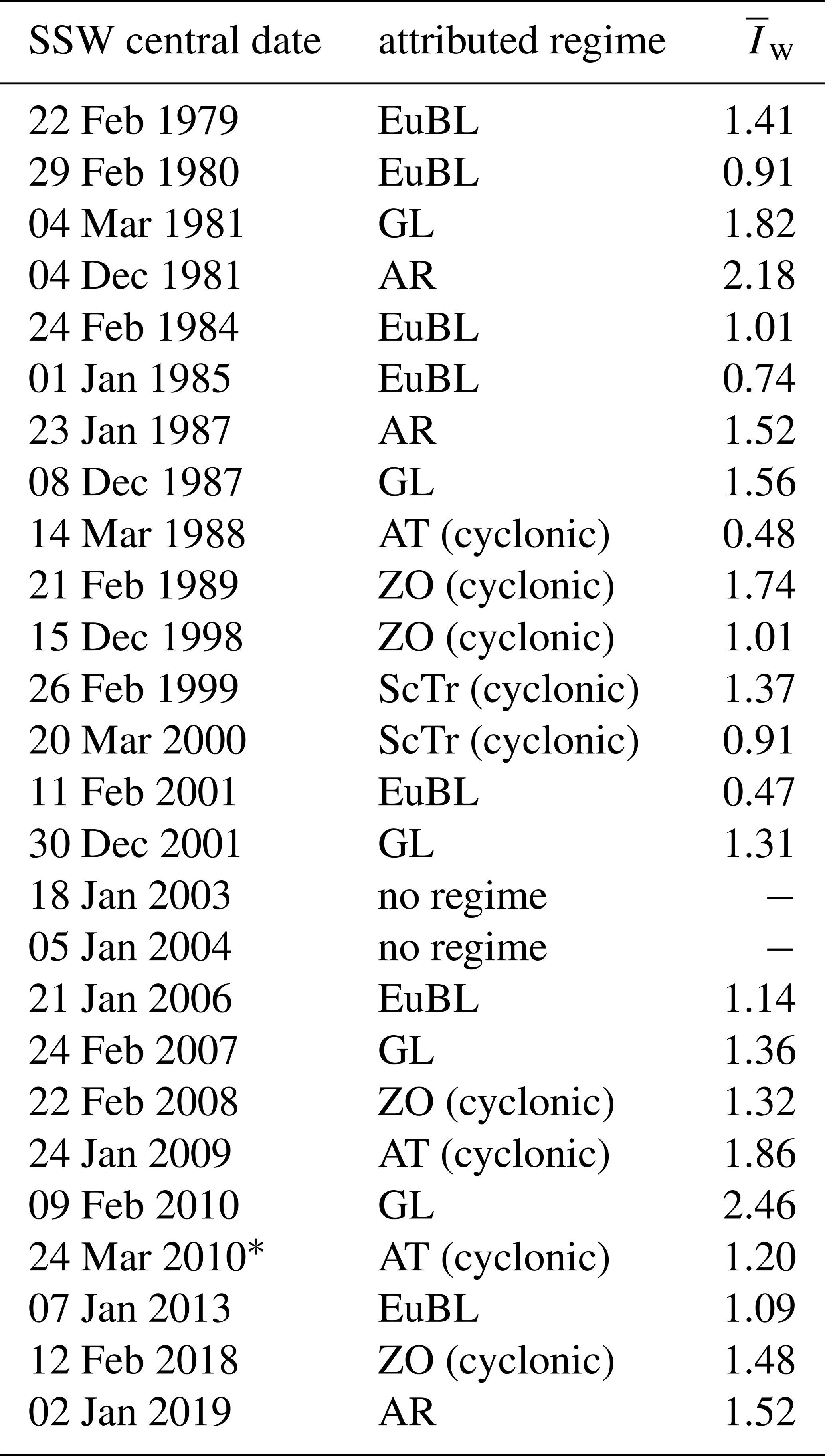
As a first step, we evaluate the sequence of weather regimes from 60 d before to 60 d after an SSW for all 26 SSW cases during 1979–2019 (Fig. 1, Table 1). Note that Fig. 1 shows the dominant persistent regime, so that alternating regimes in a time window shorter than the persistence criterion of 5 d indicate simultaneously active regime life cycles (see Sect. 2.1 for details). This figure suggests a preferred occurrence of AT (purple) and GL (blue) during the weeks after an SSW compared to the weeks before.
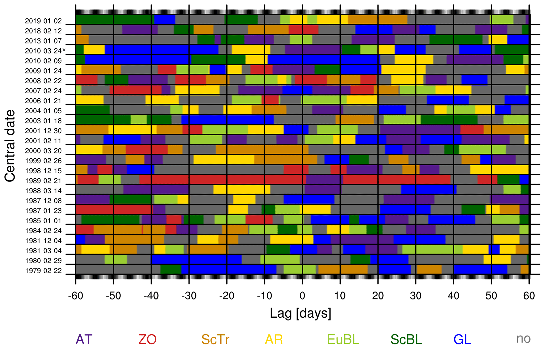
Figure 1The sequence of the dominant weather regimes (colors indicated in legend) for −60 to +60 d with respect to the onset for all 26 SSW events (lag 0) between 1979 and 2019. The central dates of the SSW events are indicated on the left. Asterisk (*) indicates that the event has been excluded from the subsequent analysis; for details see Sect. 2.1.
This is further emphasized by the 5 d running mean of the anomalous frequency of weather regimes around SSW events, which provides a more complete overview over the modulation of regime frequencies after SSWs (Fig. 2). We show the 5 d running mean frequency anomaly to account for the 5 d minimum duration of an active regime life cycle. Different from the testing procedure outlined in Sect. 2.2, we here consider the distribution of lagged 5 d mean frequencies by selecting for each day in the original sample a random day ±15 d around the original day of year but from a different winter. In addition, the random day must exhibit the same weather regime as the original day to replicate potential regime dependence. We then compute the mean lagged weather regime frequency for each random sample as for the original sample and test for significance at the 10 % level (bold). For reference, we show the absolute frequencies of weather regimes in Fig. A2.
GL and EuBL are the most prominent regimes around the onset of SSW events with a 5 d mean frequency of around 19 % and 21 %, respectively (Fig. A2a). The frequency of EuBL is significantly enhanced from 5 d prior until the onset of the SSW (Fig. 2a), in agreement with Woollings et al. (2010) and Nishii et al. (2011). The cyclonic regimes ZO and ScTr, as well as the blocked regimes AR and ScBL, tend to be suppressed at the time of SSW events. This is consistent with the strong projection of the ZO and ScTr regimes onto NAO+, which also tends to be suppressed after SSW events (Charlton-Perez et al., 2018). On the other hand, AR (yellow, significant peak around lag −20 to −10) and the related ScTr (orange, significant around lag −10) regimes are more frequent in the period 1–3 weeks before the SSW onset. The prominence of AR around 15 d before the onset of an SSW event agrees with the suggested precursor role of blocking over the Atlantic before SSW events (Martius et al., 2009). Furthermore, blocking over the Ural region in Eurasia has been suggested as a precursor to SSW events (Kolstad and Charlton-Perez, 2011; Peings, 2019; White et al., 2019). The Ural blocking precursor projects onto the EuBL and especially the ScBL regimes, which are also found to show significant positive anomalies of occurrence within the 3 weeks before SSW events (Fig. 2a). It is well known that precursors in the North Pacific also tend to be prevalent before SSW events, e.g., Garfinkel et al. (2012) and Lehtonen and Karpechko (2016), though these are not possible to identify with the present analysis, which is focused on the NAE region. After the SSW onset, AT frequencies are significantly enhanced, peaking at around 20 % after 7 d (Fig. A2a), corresponding to a frequency anomaly of around 12 % for the same lag (Fig. 2a). Thereafter, GL (lag 12 to 40 d) and AT (lag 17–35 d) are the most likely weather regimes with enhanced frequency anomalies of up to 15 % (Fig. 2a), while in absolute terms frequencies for both are around 20 %–25 % and neither of the two clearly dominates (Fig. A2a). This dominant occurrence of both GL and AT after SSW events obscures the potential tropospheric impact of an SSW in a composite, as AT and GL trigger contrasting large-scale weather conditions (mild and windy for AT, cold and calm for GL) for large parts of Europe (Beerli and Grams, 2019).
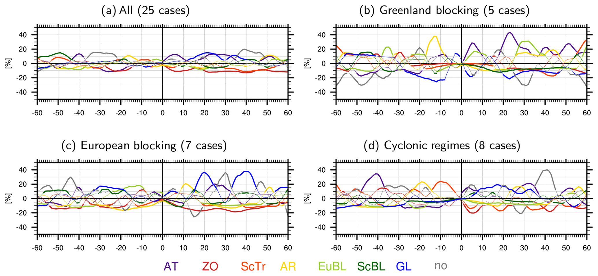
Figure 2The 5 d running mean of the anomalous frequency of weather regimes centered on the onset of the SSW event (lag 0) relative to the mean of the climatological distribution (a) for all SSW events and (b–d) conditional on the dominant weather regime around lag 0: (b) Greenland blocking, (c) European blocking, and (d) cyclonic regimes (ZO, AT, and ScTr). The 5 d mean frequencies are computed from 6-hourly weather regime data for lags of −60 to 60 d. Note that anomalous frequencies at lag 0 in (c) and (d) are – by construction – close to zero as the same regime is prescribed for computing the mean from the 1000 Monte Carlo samples. The bold parts of the lines indicate significant deviations from climatology (see text for details).
We now subdivide the 25 SSW events with respect to the weather regime that dominates during the 10 d around the SSW onset: GL (five cases), EuBL (seven cases), and the cyclonic regimes (ZO, ScTr, AT; eight cases). The remaining five cases either have no clear regime signature (no regime, two events) or are associated with AR (three events) at their onset. Because of the small sample size, we do not consider these cases here. For the GL subset (Figs. 2b, A2b), all other regimes are subsequently suppressed except for AT and EuBL. The frequency of GL itself drops immediately after the SSW, reaching values below 10 % around a lag of 20 d (Fig. A2b) – far below its climatological mean frequency. AT, and to a lesser degree also EuBL, become significantly more frequent immediately after the SSW until about a lag of 10 d, reaching absolute frequencies of 35 % and 20 %, respectively (Fig. A2b). After a period with no clear regime assignment, AT becomes the dominant regime starting at lag 18 d with anomalous frequencies above 40 % (Fig. 2b), peaking above 50 % absolute frequency about 23 d after the SSW and remaining significantly enhanced until a lag of 33 d (Fig. A2b). From lag 25 d until lag 40 d, EuBL becomes significantly enhanced, peaking at 40 % absolute frequency around lag 30 d.
For the EuBL subset (Figs. 2c, A2c), the subsequent regime frequencies are quite different to GL around the onset of an SSW. First, the frequency of AR is significantly enhanced directly after the SSW, with peaks at 30 % absolute frequency at lag 10 d. This is then followed by a period of preferred occurrence of GL (lag 15 to 25 d) and AT (lag 21 to 32 d) with an absolute frequency reaching up to 45 % and 35 %, respectively. The dominance of GL from lag 33 to 45 d (above 45 % peak frequency) is particularly striking.
Cyclonic regimes around the time of the SSW (Fig. 2d, A2d) exhibit a less prominent regime frequency modulation after an SSW compared to the EuBL and GL subsets. Still, GL (lag 5–35 d), AR (lag 24–31 d), and AT (lag 25–37 d) are significantly enhanced, but absolute frequencies remain around 20 %–30 %. Note that this corresponds to significantly increased frequencies of 10 %–20 % for these regimes in the considered time windows. However, most often no single regime dominates after an SSW event with a cyclonic regime at lag 0, hinting at cases with no downward response after the SSW event. Of the eight SSWs with cyclonic weather regimes at lag 0, Karpechko et al. (2017) investigated seven and classified five out of the seven SSW events as lacking a tropospheric impact. For EuBL and GL around the onset of the SSW, seven out of seven and one out of five, respectively, are classified as having a tropospheric impact. The reasons for this will be discussed in the next section.
Despite the large tropospheric variability in the aftermath of SSW events, the investigation of lagged regime frequencies reveals that (1) the AT and GL regimes are more likely to follow an SSW (as compared to other weather regimes) and (2) that this subsequent modulation is sensitive to the tropospheric flow regime around the onset of the SSW. The dominance of EuBL and GL at the time of the SSW onset hints at a significantly more likely GL response (after EuBL at lag 0) vs. AT (after GL at lag 0) after an SSW, respectively. Thus the stratospheric impact on the evolution of the tropospheric flow in the NAE region and hence the associated surface weather may be connected to the presence of a particular tropospheric regime around the onset of the SSW.
We focus in the following on the modulation of stratosphere–troposphere coupling for the previously discussed sets of SSWs. For that purpose, we evaluate the temporal evolution of standardized geopotential height anomalies averaged over the NAE sector (60–90∘ N, 80∘ W–40∘ E) by compositing a given set of SSW events. Using the full hemisphere, that is, the full longitude range instead of the here used longitude sector over the North Atlantic, yields the same qualitative results due to the strong imprint of the anomalies induced by the SSW in the NAE sector (Fig. A3).
Compositing all SSW events (Fig. 3a) yields the classical dripping paint plot of Baldwin and Dunkerton (2001, their Fig. 2). Qualitative differences compared to the figure from Baldwin and Dunkerton (2001) are due to the different variable (geopotential height in our study vs. northern annular mode, NAM) and the number of events (25 in our study vs. 18) for a different time period (1979–2019 in our study vs. 1958–1999). When compositing all SSW events, the downward impact between 10 and 60 d after the SSW onset is robust at the 25 % but not the 10 % level (see Fig. A4a). Together with the relatively weak amplitude of the anomalies, this reflects the large case-to-case variability in the tropospheric impact of SSWs. Despite the low robustness, the anomaly around a lag of 15 d is unlikely to be obtained from a random sampling as evident from the less than 10 % overlap between the confidence and random distributions (Fig. 3a). This suggests that in the aftermath of an SSW (lag 15–25 d), indeed positive geopotential height anomalies over the NAE sector are significantly more likely than in the absence of an SSW.
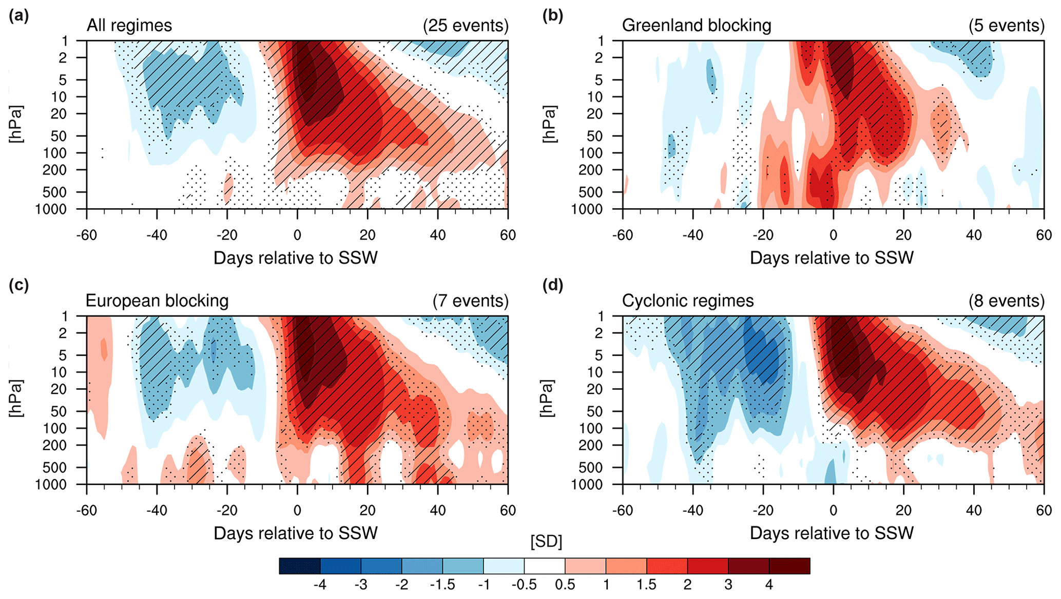
Figure 3Standardized geopotential height anomalies for the North Atlantic sector (60–90∘ N, 80∘ W–40∘ E) (a) for all SSW events and (b–d) subdivided by the weather regime that is dominant around the onset of the SSW event as indicated in the panel titles. Stippling (hatching) indicates that the confidence intervals and the random distributions overlap by less than 25 % (10 %). Figure A3 shows a version of this figure for the full longitude range.
SSW events that occur during GL (Fig. 3b) are associated with an immediate, strongly positive anomaly in the troposphere. Consistent with Fig. A2b, when GL is present around the onset of the SSW, GL or AR are often already present before the SSW event, which is likely the cause of the positive tropospheric geopotential height anomalies several days prior to the event. Notably, there are no significant and robust (Figs. 3b and A4b) anomalies after 10 d of the onset of the SSW except for a weak negative geopotential height anomaly after 20 d (significant at the 25 % level), indicating a cyclonic flow regime in the NAE region. This is consistent with the significantly enhanced likelihood for the occurrence of the AT regime at this lag (Fig. A2b). Note that both the immediate positive geopotential height anomalies and the weak tropospheric anomalies in the aftermath of the event are not the result of cancellations in the composites but are rather typical across cases. In fact, four out of the here identified five GL events have been classified by Karpechko et al. (2017) as having no downward impact.
For EuBL around the onset of the SSW event, a robust (10 % level) positive tropospheric anomaly can be observed at the time of the SSW (Fig. A4c). This anomaly is not significant (Fig. 3c), reflecting that it is not different from generic anomalies during EuBL. However, robust, significant, and strongly positive geopotential height anomalies are present in the troposphere at lags of 15–20 and 30–55 d after the SSW event. This is consistent with the classification of all of the here defined seven EuBL events as having a tropospheric impact in Karpechko et al. (2017). These positive anomalies are consistent with the finding that first AR and then GL are much more likely in the aftermath of an SSW with EuBL around lag 0 (compare to Fig. A2c). Furthermore, comparing to the panel for all SSW events (Fig. 3a) indicates that the EuBL cases dominate the perceived downward response in the canonical response for SSW events.
During cyclonic regimes around the onset of the SSW, there is no substantial tropospheric anomaly in the NAE region at the time of the SSW, but a positive albeit weak anomaly can be observed around days 15–20 after the SSW event (Fig. 3d). This anomaly is not robust at the 25 % level, but it is significantly different from a random sample at the 25 % level (Fig. A4d). Several SSWs with a cyclonic regime around the onset are followed by GL at a longer lag (Fig. A2d), thus likely causing these anomalies. Still, the GL absolute frequencies remain below 30 % (Fig. A2). These findings and the small amplitude of the anomalies suggest that the variability in the tropospheric flow evolution after SSWs is large after a cyclonic regime at lag 0, which is also confirmed by the inspection of individual cases (not shown).
The question arises of whether other factors might contribute to the differing tropospheric evolution in the aftermath of the SSW event. In particular, a differing amplitude and persistence of the lower stratospheric anomaly can be observed in Fig. 3 between the different composites. Events with EuBL around the onset and a strong downward impact tend to have a longer stratospheric persistence, but an equally long persistence can be observed for cyclonic regimes around the onset of the SSW, with little downward impact. The five SSW events associated with GL have a shorter-lived lower stratospheric response. As events with a persistent lower stratospheric response are often associated with so-called polar jet oscillation (PJO) events (Kuroda and Kodera, 2004; Hitchcock et al., 2013b), a comparison with Table 1 in Karpechko et al. (2017) reveals that two out of five SSW events with a GL regime (and, respectively, four out of seven EuBL events) around the onset are associated with a PJO event. While this is not a clear result, it indicates that the shorter (longer) persistence in the lower stratosphere for the SSWs associated with GL (EuBL) may add support to the persistence of the tropospheric response for several of the events, but the statistics are too small to provide a clear result. Similarly, four out of seven EuBL events are split events (rather than displacements), while two out of five GL events are split events, according to the classification in Karpechko et al. (2017).
Since each weather regime is associated with characteristic surface weather, the modulation of regime successions in the aftermath of an SSW by the tropospheric state at the time of an SSW might contribute to the marked variability in the surface impact. Hence, we here consider spatial composites of anomalies of 2 m temperature (T2m') and 500 hPa geopotential height (Z500') for the three groups of SSW events discussed in the previous sections (Fig. 4a–c) and for all SSW events (Fig. 4d) for days 0 to 25 after the SSW (Fig. A5 for days 25–50).
During SSWs dominated by GL around their onset, initially strongly positive T2m' values prevail over Greenland and the Canadian Archipelago, whereas western Russia and Scandinavia are anomalously cold, consistent with the anomalous ridge over Greenland and the low geopotential height anomalies over Scandinavia (Fig. 4a). With the subsequent progression of weather regimes – typically towards the cyclonic AT regime or EuBL – mild conditions are established throughout central Europe from a lag of 20 d onwards. This is in stark contrast to the negative NAO phase and the associated cold conditions that are commonly expected as the canonical response to SSWs over Europe (Butler et al., 2017; Kolstad et al., 2010; Domeisen et al., 2020a).
For SSWs that are dominated by EuBL around their onset, cold anomalies prevail over northern Europe, albeit also extending over large parts of central Europe (Fig. 4b). They peak at −4 to −6 K around lags beyond 20 d, which corresponds well with the occurrence of the GL regime. Note that negative T2m' values in the composite for all SSWs are much weaker (see Fig. 4d). The associated retrogression of initial positive Z500' over the eastern North Atlantic to Greenland along with a strengthening of negative Z500' over the southeastern North Atlantic around lag 15–25 d is striking. Furthermore, GL is associated with warm anomalies over Greenland and eastern Canada.
Finally, as expected by the varied regime succession for the SSWs with cyclonic regimes at their onset, composite T2m and Z500 anomalies are weaker for these events (Fig. 4c). Thus, the canonical response of surface temperature (i.e., the composite for all SSWs, Fig. 4d) is the result of averaging over – in important regions opposing – temperature anomalies for SSWs with GL, EuBL, or a cyclonic regime around the onset.
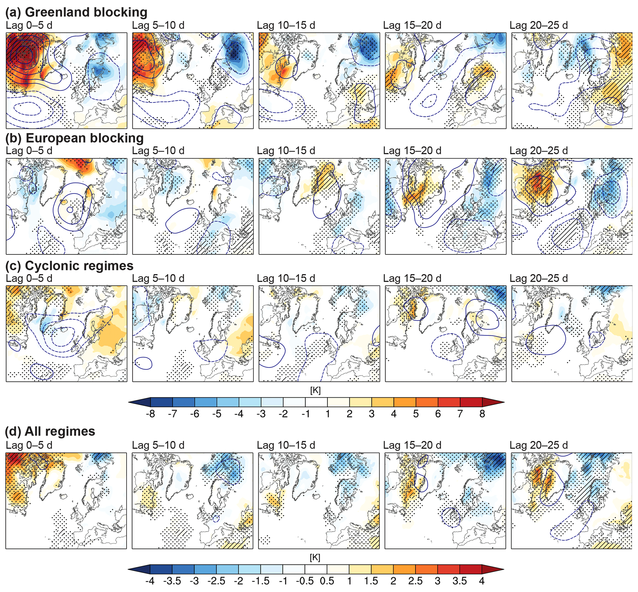
Figure 4Surface impact for SSWs with (a) Greenland blocking, (b) European blocking, and (c) cyclonic regimes around the SSW onset, as well as (d) for all SSWs. Shading indicates the composite 2 m temperature anomalies, with stippling (hatching) indicating significance at the 25 % (10 %) level. Blue contours correspond to geopotential height anomalies at 500 hPa in intervals of 50 gpm (geopotential meters). Negative values are dashed. The fields are averaged over 5 d between lags 0 and 25 d with respect to the SSW central date. Note the different scales for temperature in (a)–(c) and (d). The 2 m temperature anomalies are detrended and deseasonalized using 9-year and 21 d running mean filters.
This study aimed to shed light on the large case-to-case variability of the tropospheric response to SSW events and their associated surface impacts, as well as the dependence on the tropospheric weather regime around the onset of the SSW. To that end, we have exploited in a statistical framework the observational record of the satellite era (1979–2019) as represented in the ERA-Interim reanalysis. Our conclusions are as follows:
-
In the aftermath of an SSW event, the tropospheric flow in the NAE region exhibits an evolution that is unlikely to occur in the absence of an SSW. Specifically, positive geopotential height anomalies related to Greenland blocking are statistically more likely to occur after the onset of the SSW than in the absence of an SSW. This is consistent with the expected (canonical) negative NAO response of the troposphere to SSWs (e.g., Charlton-Perez et al., 2018).
-
The significant and robust positive geopotential height anomalies found in the period 10–60 d after SSWs are predominantly the result of SSWs with European blocking dominating around their onset. This is manifested for this subset of events in a transition from EuBL to GL that then dominates at lags of 15–20 and 30–55 d after the SSW onset, which is statistically significantly different from the natural progression from EuBL to GL. These events all correspond to SSWs that have in the literature been classified as having a tropospheric response (e.g., Karpechko et al., 2017). For other tropospheric regimes at SSW onset the tropospheric response is weaker and less robust and significant.
-
For Greenland blocking at the SSW onset, a weak preference for cyclonic flow regimes around 20–30 d after the SSW is apparent, with an opposite surface response in the aftermath of the SSW as compared to SSW onsets dominated by EuBL. These events almost exclusively correspond to SSWs that have in the literature been classified as having no tropospheric response.
-
SSWs that occur during cyclonic weather regimes exhibit a considerably weaker and less significant response as compared to SSW events associated with EuBL, with a modestly enhanced likelihood for GL.
Depending on the tropospheric weather regime around the SSW onset, different surface signatures result. Specifically, the signature in 2 m temperature resembling the expected canonical NAO− state, e.g., cold conditions prevailing over much of northern Europe, occurs for the EuBL cases. In contrast, mild temperatures in large parts of Europe are found for SSWs with GL around their onset. It is important to distinguish these cases, since although EuBL and GL frequently (that is, for roughly 50 % of all SSWs) occur around the onset of SSW events, they lead to a different subsequent evolution and different associated surface temperatures. In particular, the most common SSW events exhibit a transition from EuBL (GL) around SSW onset to GL (AT) around 3–4 weeks after the SSW, respectively, along with their contrasting large-scale weather impacts (Beerli and Grams, 2019). Note that these differences cannot be identified by using a set limited to four weather regimes. These findings indicate that the presence of either a EuBL or GL regime at SSW onset will allow us to disentangle the difference in surface weather and hence to determine if and when a downward impact of the SSW is expected. This is highly relevant for subseasonal forecasting.
While these findings are limited by the small sample size of SSW events available in the observational record, the rigorous statistical testing for significance and robustness performed here suggests that the large case-to-case variability in the tropospheric response to SSWs can be described in terms of NAE weather regimes and may depend on the regime around the onset of the SSW for many of the observed SSWs. Our findings confirm that while the stratosphere does not represent the sole forcing of the tropospheric state, for many SSW events it is able to affect the tropospheric flow by suppressing some weather regimes and by favoring others, as found in Charlton-Perez et al. (2018). We here in addition show that the susceptibility of the troposphere to the stratospheric forcing depends on the tropospheric state around the time of the SSW. Other factors that can modulate the tropospheric response to SSW events are the persistence of the temperature anomaly in the lower stratosphere (Hitchcock et al., 2013a; Karpechko et al., 2017; Runde et al., 2016; Polichtchouk et al., 2018), as well as upstream effects in the North Pacific (Afargan-Gerstman and Domeisen, 2020; Jiménez-Esteve and Domeisen, 2018). An analysis of differences in the lower stratospheric persistence for the weather regimes considered here did not yield conclusive results, which warrants further studies. Note that it was not possible in our analysis to fully exclude differences in the stratospheric forcing between SSW events due to the small sample size. In particular, differences in stratospheric behavior, such as vortex geometry or the persistence of the temperature signal in the lower stratosphere, may influence the type and persistence of the downward response. We expect a negligible influence from the vortex geometry, as the differences in the surface signals between split and displacement events tend to be small (Charlton and Polvani, 2007; Mitchell et al., 2013; Maycock and Hitchcock, 2015; Seviour et al., 2016; Lehtonen and Karpechko, 2016) and are also affected by the small sample size. While the persistence of the lower stratospheric response likely affects the persistence and type of the tropospheric signal (Hitchcock et al., 2013a; Karpechko et al., 2017; Runde et al., 2016; Polichtchouk et al., 2018), we did not find a clear correspondence between persistent stratospheric events and tropospheric weather regime evolution. In particular, roughly half of SSW events associated with either EuBL (4 out of 7) or GL (2 out of 5) are associated with a persistent lower stratospheric response (note the small sample size). Hence, we could not find a clear equivalence between tropospheric weather regimes and lower stratospheric persistence.
Our goal is to emphasize that the troposphere has a role to play in the downward response of SSW events. The respective contributions of the stratosphere, the state of the troposphere over the North Atlantic, and upstream precursors will subsequently have to be disentangled in a modeling study. In particular, a model study to quantify the respective contributions to the tropospheric impact of different remote factors in comparison to the role of local North Atlantic variability might shed further light onto the complex role of stratosphere–troposphere coupling for surface weather. However, it is currently not sufficiently known to what extent complex prediction models are able to represent the diversity of tropospheric responses to stratospheric forcing, as this has not been sufficiently tested in models beyond the canonical response and selected case studies. From a preliminary analysis of subseasonal prediction models we anticipate large biases and a complex role of the representation of stratosphere–troposphere coupling in prediction models that will be difficult to disentangle. Hence, while state-of-the-art subseasonal prediction systems are often unable to forecast at the time of occurrence of the SSW event if a surface response is to be expected, our findings suggests that the presence or absence – and in fact the timing – of a surface impact following SSW events might in some cases be predictable based on the dominant weather regime around the onset of the SSW event. This could significantly improve the subseasonal prediction of tropospheric winter weather following SSW events over Europe.
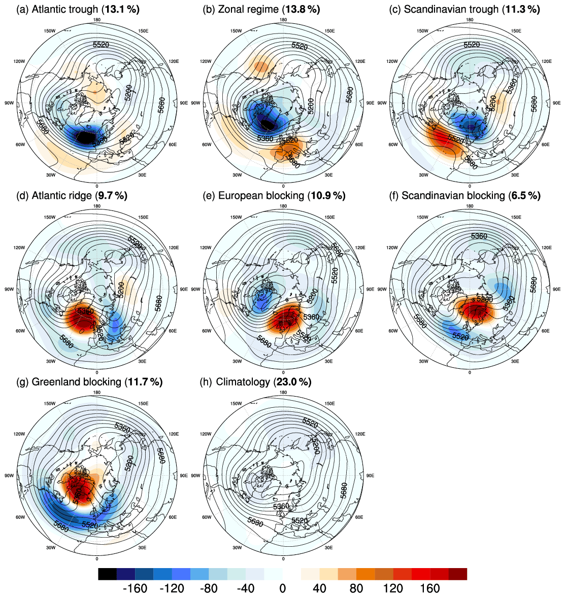
Figure A1Composite mean 10 d low-pass-filtered 500 hPa geopotential height anomaly (shading, every 20 gpm), and mean absolute 500 hPa geopotential height (black contours, every 20 gpm) for all winter days in ERA-Interim (DJF, 1979–2015) attributed to one of the seven weather regimes (a–g) and the climatological mean (h). Regime name and relative frequency (in percent) are indicated in the subfigure captions.
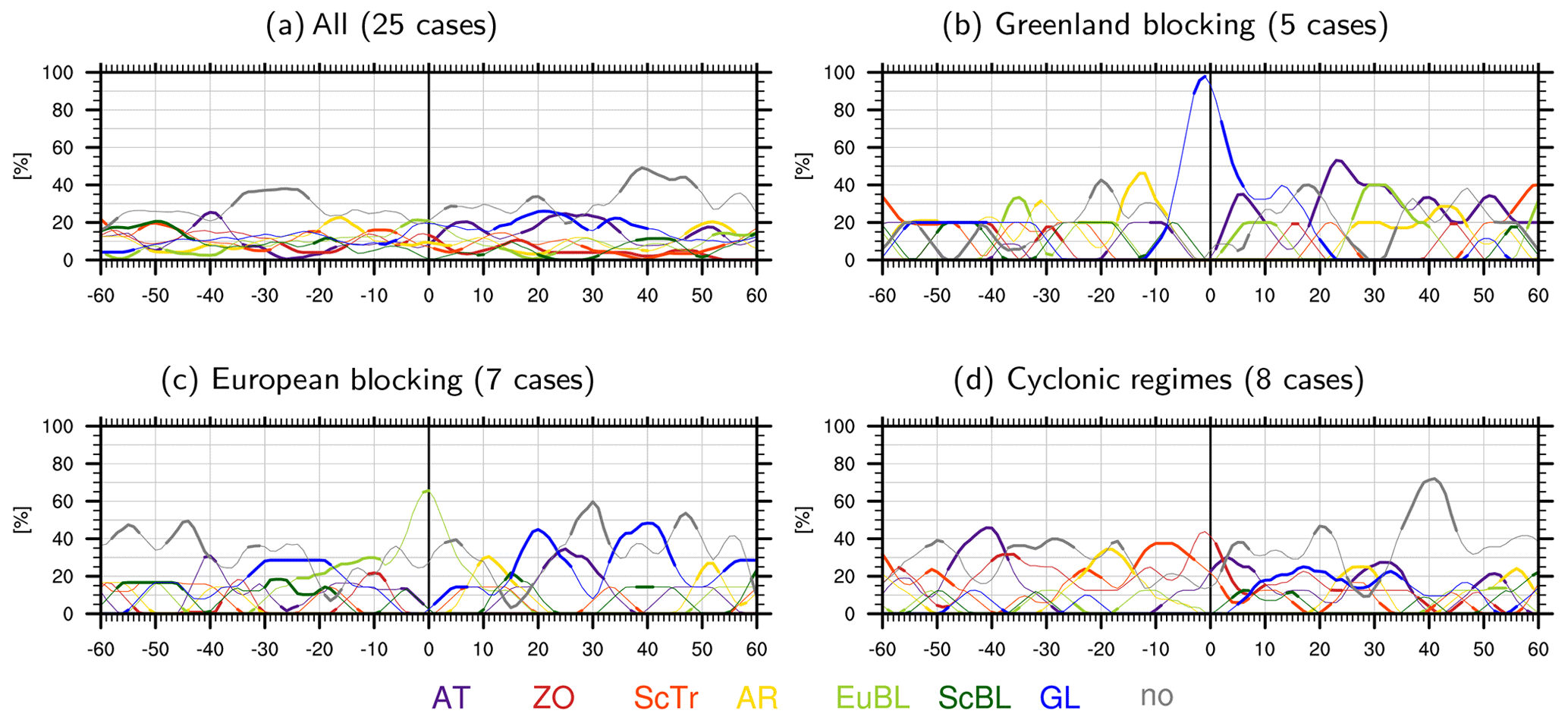
Figure A2As Fig. 2 but for the 5 d running mean absolute frequency of weather regimes centered on the onset of the SSW event (lag 0) for (a) all SSW events and (b–d) conditional on the dominant weather regime at lag 0: (b) Greenland blocking, (c) European blocking, and (d) cyclonic regimes (ZO, AT, and ScTr). The 5 d mean frequencies are computed from 6-hourly weather regime data from lag −60 d to lag 60 d. The bold parts of the lines indicate significant deviations from climatology (see text for details).
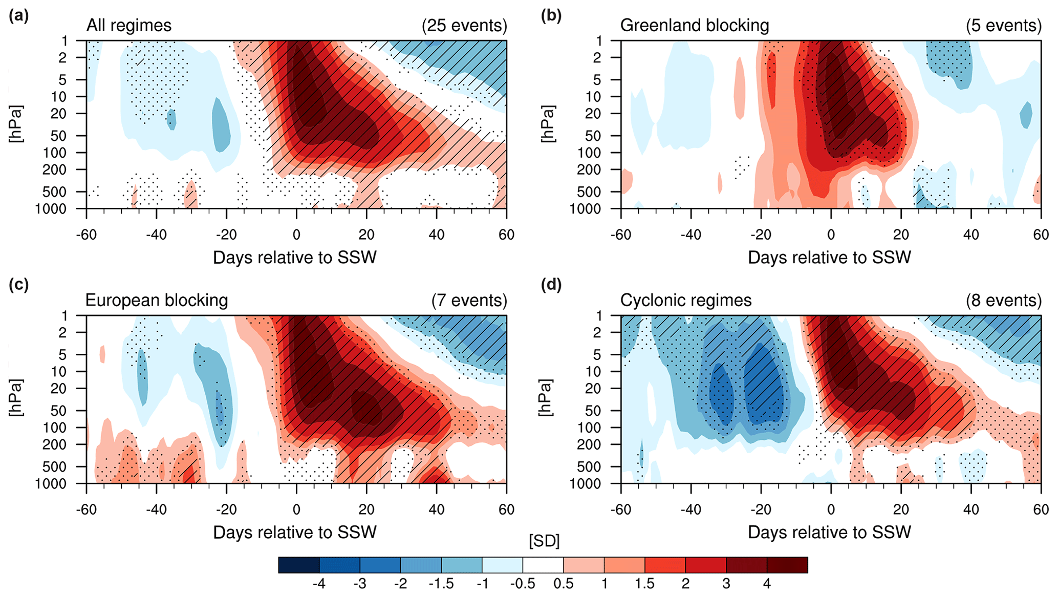
Figure A3As Fig. 3 but for the full longitude range, i.e., for the polar cap poleward of 60∘ N.

Figure A4Standardized geopotential height anomalies for the sector (60–90∘ N, 80∘ W–40∘ E) (a) for all SSW events and (b–d) subdivided by the weather regime that is dominant around the onset of the SSW as indicated by the titles of the panels. Robustness is assessed using confidence intervals by resampling the SSW events 100 times with repetition. If the magnitude of the anomaly exceeds the interquartile or the 10th–90th percentile ranges, the anomaly is highlighted by stippling or hatching, respectively. See Sect. 2.2 for details.
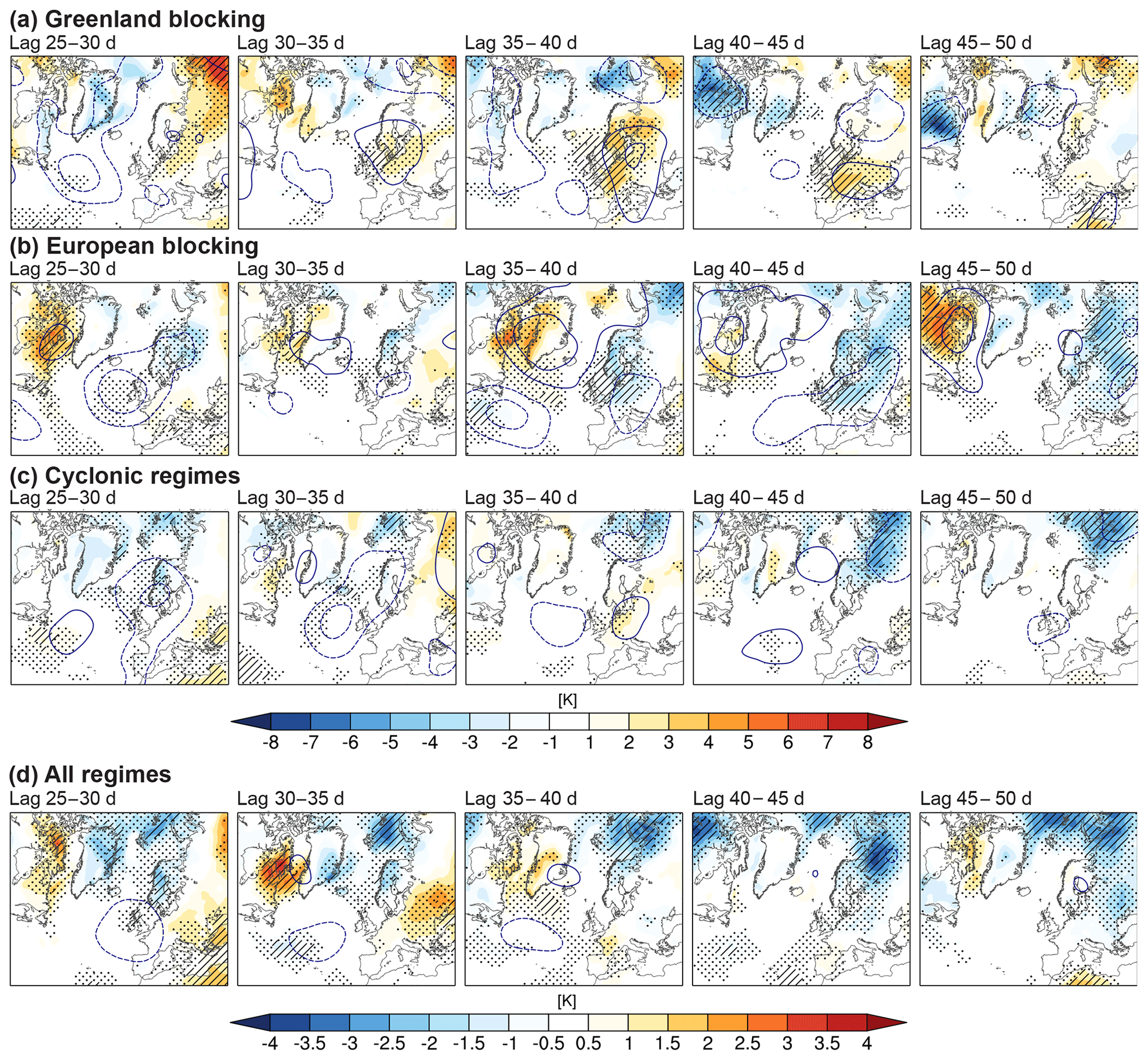
Figure A5As Fig. 4 but for days 25–50.
The ERA-Interim reanalysis data (Dee et al., 2011) are available from ECMWF at https://apps.ecmwf.int/datasets/data/interim-full-daily/ (last access: 7 August 2020).
The authors together initiated and designed the study, and all authors contributed to data analysis, discussion of results, and writing.
The authors declare that they have no conflict of interest.
Data analysis and visualization were performed using the NCAR Command Language (UCAR/NCAR/CISL/VETS, 2014). The authors thank the editor Pedram Hassanzadeh and the three anonymous reviewers for their reviews of the manuscript.
Support was provided by the Swiss National Science Foundation through project PP00P2_170523 to Daniela I. V. Domeisen. The contribution of Christian M. Grams was supported by the Helmholtz Association as part of the Young Investigator Group “SPREADOUT” (grant no. VH-NG-1243).
This paper was edited by Pedram Hassanzadeh and reviewed by three anonymous referees.
Afargan-Gerstman, H. and Domeisen, D. I. V.: Pacific Modulation of the North Atlantic Storm Track Response to Sudden Stratospheric Warming Events, Geophys. Res. Lett., 47, e2019GL085007, https://doi.org/10.1029/2019GL085007, 2020. a, b
Andrews, M. B., Knight, J. R., Scaife, A. A., and Lu, Y.: Observed and simulated teleconnections between the stratospheric Quasi-Biennial Oscillation and Northern Hemisphere winter atmospheric circulation, J. Geophys. Res.-Atmos., 124, 1219–1232, https://doi.org/10.1029/2018JD029368, 2019. a
Attard, H. E., Lang, A. L., Attard, H. E., and Lang, A. L.: The Impact of Tropospheric and Stratospheric Tropical Variability on the Location, Frequency, and Duration of Cool-Season Extratropical Synoptic Events, Mon. Weather Rev., 147, 519–542, 2019. a
Ayarzagüena, B., Barriopedro, D., Perez, J. M. G., Abalos, M., de la Camara, A., Herrera, R. G., Calvo, N., and Ordóñez, C.: Stratospheric Connection to the Abrupt End of the 2016/2017 Iberian Drought, Geophys. Res. Lett., 45, 12639–12646, 2018. a
Baldwin, M. P. and Dunkerton, T. J.: Stratospheric harbingers of anomalous weather regimes, Science, 294, 581–584, 2001. a, b, c
Barnes, E. A., Samarasinghe, S. M., Uphoff, I. E., and Furtado, J. C.: Tropospheric and Stratospheric Causal Pathways Between the MJO and NAO, J. Geophys. Res.-Atmos., 124, 9356–9371, 2019. a
Beerli, R. and Grams, C. M.: Stratospheric Modulation of the Large-Scale Circulation in the Atlantic-European Region and Its Implications for Surface Weather Events, Q. J. Roy. Meteor. Soc., 145, 3732–3750, https://doi.org/10.1002/qj.3653, 2019. a, b, c, d
Beerli, R., Wernli, H., and Grams, C. M.: Does the lower stratosphere provide predictability for month-ahead wind electricity generation in Europe?, Q. J. Roy. Meteor. Soc., 143, 3025–3036, 2017. a
Butler, A., Charlton-Perez, A., Domeisen, D. I. V., Garfinkel, C., Gerber, E. P., Hitchcock, P., Karpechko, A. Y., Maycock, A. C., Sigmond, M., Simpson, I., and Son, S.-W.: Sub-seasonal Predictability and the Stratosphere, in: Sub-Seasonal to Seasonal Prediction, Elsevier, 223–241, https://doi.org/10.1016/B978-0-12-811714-9.00011-5, 2019. a
Butler, A. H., Arribas, A., Athanassiadou, M., Baehr, J., Calvo, N., Charlton-Perez, A., Déqué, M., Domeisen, D. I. V., Fröhlich, K., Hendon, H., Imada, Y., Ishii, M., Iza, M., Karpechko, A. Y., Kumar, A., MacLachlan, C., Merryfield, W. J., Müller, W. A., O'Neill, A., Scaife, A. A., Scinocca, J., Sigmond, M., Stockdale, T. N., and Yasuda, T.: The Climate-system Historical Forecast Project: do stratosphere-resolving models make better seasonal climate predictions in boreal winter?, Q. J. Roy. Meteor. Soc., 142, 1413–1427, 2016. a
Butler, A. H., Sjoberg, J. P., Seidel, D. J., and Rosenlof, K. H.: A sudden stratospheric warming compendium, Earth Syst. Sci. Data, 9, 63–76, https://doi.org/10.5194/essd-9-63-2017, 2017. a, b, c, d, e
Cassou, C.: Intraseasonal interaction between the Madden–Julian oscillation and the North Atlantic Oscillation, Nature, 455, 523–527, https://doi.org/10.1038/nature07286, 2008. a
Charlton, A. and Polvani, L.: A new look at stratospheric sudden warmings. Part I: Climatology and modeling benchmarks, J. Climate, 20, 449–469, 2007. a, b
Charlton-Perez, A. J., Ferranti, L., and Lee, R. W.: The influence of the stratospheric state on North Atlantic weather regimes, Q. J. Roy. Meteor. Soc., 144, 1140–1151, 2018. a, b, c, d, e, f, g, h
Cohen, J., Furtado, J. C., Jones, J., Barlow, M., Whittleston, D., and Entekhabi, D.: Linking Siberian Snow Cover to Precursors of Stratospheric Variability, J. Climate, 27, 5422–5432, 2014. a
Cropper, T., Hanna, E., Valente, M. A., and Jónsson, T.: A daily Azores-Iceland North Atlantic Oscillation index back to 1850, Geosci. Data J., 2, 12–24, 2015. a
Dee, D., Uppala, S., Simmons, A., Berrisford, P., Poli, P., Kobayashi, S., Andrae, U., Balmaseda, M., Balsamo, G., Bauer, P., Bechtold, P., Beljaars, A., Berg, L., Bidlot, J., Bormann, N., Delsol, C., Dragani, R., Fuentes, M., Geer, A., Haimberger, L., Healy, S., Hersbach, H., Holm, E., Isaksen, L., Kållberg, P., Köhler, M., Matricardi, M., McNally, A., Monge-Sanz, B., Morcrette, J., Park, B., Peubey, C., Rosnay, P. D., Tavolato, C., Thepaut, J., and Vitart, F.: The ERA-Interim reanalysis: Configuration and performance of the data assimilation system, Q. J. Roy. Meteor. Soc., 137, 553–597, https://doi.org/10.1002/qj.828, 2011. a, b
Domeisen, D. I. V.: Estimating the Frequency of Sudden Stratospheric Warming Events from Surface Observations of the North Atlantic Oscillation, J. Geophys. Res.-Atmos., 124, 3180–3194, https://doi.org/10.1029/2018JD030077, 2019. a, b, c
Domeisen, D. I. V., Sun, L., and Chen, G.: The role of synoptic eddies in the tropospheric response to stratospheric variability, Geophys. Res. Lett., 40, 4933–4937, https://doi.org/10.1002/grl.50943, 2013. a
Domeisen, D. I. V., Butler, A. H., Fröhlich, K., Bittner, M., Müller, W. A., and Baehr, J.: Seasonal Predictability over Europe Arising from El Niño and Stratospheric Variability in the MPI-ESM Seasonal Prediction System, J. Climate, 28, 256–271, https://doi.org/10.1175/JCLI-D-14-00207.1, 2015. a
Domeisen, D. I. V., Badin, G., and Koszalka, I. M.: How Predictable Are the Arctic and North Atlantic Oscillations? Exploring the Variability and Predictability of the Northern Hemisphere, J. Climate, 31, 997–1014, 2018. a
Domeisen, D. I. V., Garfinkel, C. I., and Butler, A. H.: The Teleconnection of El Niño Southern Oscillation to the Stratosphere, Rev. Geophys., 57, 5–47, https://doi.org/10.1029/2018RG000596, 2019. a
Domeisen, D. I. V., Butler, A. H., Charlton-Perez, A. J., Ayarzaguena, B., Baldwin, M. P., Dunn Sigouin, E., Furtado, J. C., Garfinkel, C. I., Hitchcock, P., Karpechko, A. Y., Kim, H., Knight, J., Lang, A. L., Lim, E.-P., Marshall, A., Roff, G., Schwartz, C., Simpson, I. R., Son, S.-W., and Taguchi, M.: The role of the stratosphere in subseasonal to seasonal prediction: 2. Predictability arising from stratosphere – troposphere coupling, J. Geophys. Res.-Atmos., 125, e2019JD030923, https://doi.org/10.1029/2019JD030923, 2020a. a, b
Domeisen, D. I. V., Butler, A. H., Charlton-Perez, A. J., Ayarzaguena, B., Baldwin, M. P., Dunn Sigouin, E., Furtado, J. C., Garfinkel, C. I., Hitchcock, P., Karpechko, A. Y., Kim, H., Knight, J., Lang, A. L., Lim, E.-P., Marshall, A., Roff, G., Schwartz, C., Simpson, I. R., Son, S.-W., and Taguchi, M.: The role of the stratosphere in subseasonal to seasonal prediction: 1. Predictability of the stratosphere, J. Geophys. Res.-Atmos., 125, e2019JD030920, https://doi.org/10.1029/2019JD030920, 2020b. a
Drouard, M., Rivière, G., Arbogast, P., Drouard, M., Rivière, G., and Arbogast, P.: The North Atlantic Oscillation Response to Large-Scale Atmospheric Anomalies in the Northeastern Pacific, J. Atmos. Sci., 70, 2854–2874, 2013. a
Ferranti, L., Corti, S., and Janousek, M.: Flow-Dependent Verification of the ECMWF Ensemble over the Euro-Atlantic Sector, Q. J. Roy. Meteor. Soc., 141, 916–924, https://doi.org/10.1002/qj.2411, 2015. a, b
Garfinkel, C. I., Butler, A. H., Waugh, D. W., Hurwitz, M. M., and Polvani, L. M.: Why might stratospheric sudden warmings occur with similar frequency in El Niño and La Niña winters?, J. Geophys. Res., 117, D19106, https://doi.org/10.1029/2012JD017777, 2012. a
Garfinkel, C. I., Waugh, D. W., and Gerber, E. P.: The Effect of Tropospheric Jet Latitude on Coupling between the Stratospheric Polar Vortex and the Troposphere, J. Climate, 26, 2077–2095, 2013. a
Garfinkel, C. I., Benedict, J. J., and Maloney, E. D.: Impact of the MJO on the boreal winter extratropical circulation, Geophys. Res. Lett., 41, 6055–6062, 2014. a
Gerber, E. P., Orbe, C., and Polvani, L. M.: Stratospheric influence on the tropospheric circulation revealed by idealized ensemble forecasts, Geophys. Res. Lett., 36, L24801, https://doi.org/10.1029/2009GL040913, 2009. a
Grams, C. M., Beerli, R., Pfenninger, S., Staffell, I., and Wernli, H.: Balancing Europe's wind-power output through spatial deployment informed by weather regimes, Nat. Clim. Change, 7, nclimate3338–562, 2017. a, b
Gray, L. J., Anstey, J. A., Kawatani, Y., Lu, H., Osprey, S., and Schenzinger, V.: Surface impacts of the Quasi Biennial Oscillation, Atmos. Chem. Phys., 18, 8227–8247, https://doi.org/10.5194/acp-18-8227-2018, 2018. a
Greatbatch, R. J., Gollan, G., Jung, T., and Kunz, T.: Factors influencing Northern Hemisphere winter mean atmospheric circulation anomalies during the period 1960/61 to 2001/02, Q. J. Roy. Meteor. Soc., 138, 1970–1982, 2012. a
Hitchcock, P. and Simpson, I. R.: The Downward Influence of Stratospheric Sudden Warmings, J. Atmos. Sci., 71, 3856–3876, 2014. a
Hitchcock, P., Shepherd, T. G., and Manney, G. L.: Statistical Characterization of Arctic Polar-Night Jet Oscillation Events, J. Climate, 26, 2096–2116, 2013a. a, b, c
Hitchcock, P., Shepherd, T. G., Taguchi, M., Yoden, S., and Noguchi, S.: Lower-stratospheric Radiative Damping and Polar-night Jet Oscillation Events, J. Atmos. Sci., 70, 1391–1408, 2013b. a
Honda, M. and Nakamura, H.: Interannual Seesaw between the Aleutian and Icelandic Lows. Part II: Its Significance in the Interannual Variability over the Wintertime Northern Hemisphere, J. Climate, 14, 4512–4529, 2001. a
Huang, J. and Tian, W.: Eurasian Cold Air Outbreaks under Different Arctic Stratospheric Polar Vortex Strength, J. Atmos. Sci., 76, 1245–1264, https://doi.org/10.1175/JAS-D-18-0285.1, 2019. a
Jia, L., Yang, X., Vecchi, G., Gudgel, R., Delworth, T., Fueglistaler, S., Lin, P., Scaife, A. A., Underwood, S., and Lin, S.-J.: Seasonal Prediction Skill of Northern Extratropical Surface Temperature Driven by the Stratosphere, J. Climate, 30, 4463–4475, 2017. a
Jiménez-Esteve, B. and Domeisen, D. I. V.: The Tropospheric Pathway of the ENSO-North Atlantic Teleconnection, J. Climate, 31, 4563–4584, https://doi.org/10.1175/JCLI-D-17-0716.1, 2018. a, b
Karpechko, A. Y.: Improvements in statistical forecasts of monthly and two-monthly surface air temperatures using a stratospheric predictor, Q. J. Roy. Meteor. Soc., 141, 2444–2456, 2015. a
Karpechko, A. Y., Hitchcock, P., Peters, D. H. W., and Schneidereit, A.: Predictability of downward propagation of major sudden stratospheric warmings, Q. J. Royal Met. Soc., 104, 30937, https://doi.org/10.1002/qj.3017, 2017. a, b, c, d, e, f, g, h, i, j
Kodera, K., Mukougawa, H., Maury, P., Ueda, M., and Claud, C.: Absorbing and reflecting sudden stratospheric warming events and their relationship with tropospheric circulation, J. Geophys. Res.-Atmos., 121, 80–94, 2016. a, b
Kolstad, E. W. and Charlton-Perez, A. J.: Observed and simulated precursors of stratospheric polar vortex anomalies in the Northern Hemisphere, Clim. Dynam., 37, 1443–1456, 2011. a
Kolstad, E. W., Breiteig, T., and Scaife, A. A.: The association between stratospheric weak polar vortex events and cold air outbreaks in the Northern Hemisphere, Q. J. Roy. Meteor. Soc., 136, 886–893, 2010. a, b
Kretschmer, M., Cohen, J., Matthias, V., Runge, J., and Coumou, D.: The Different Stratospheric Influence on Cold-Extremes in Eurasia and North America, npj Climate and Atmospheric Science, 1, 44, https://doi.org/10.1038/s41612-018-0054-4, 2018a. a
Kretschmer, M., Coumou, D., Agel, L., Barlow, M., Tziperman, E., and Cohen, J.: More-Persistent Weak Stratospheric Polar Vortex States Linked to Cold Extremes, B. Am. Meteorol. Soc., 99, 49–60, 2018b. a
Kuroda, Y. and Kodera, K.: Role of the Polar-night Jet Oscillation on the formation of the Arctic Oscillation in the Northern Hemisphere winter, J. Geophys. Res., 109, D11112, https://doi.org/10.1029/2003JD004123, 2004. a
Lehtonen, I. and Karpechko, A. Y.: Observed and modeled tropospheric cold anomalies associated with sudden stratospheric warmings, J. Geophys. Res.-Atmos., 121, 1591–1610, 2016. a, b, c
Martius, O., Polvani, L., and Davies, H.: Blocking precursors to stratospheric sudden warming events, Geophys. Res. Lett., 36, L14806, https://doi.org/10.1029/2009GL038776, 2009. a
Matthias, V. and Kretschmer, M.: The Influence of Stratospheric Wave Reflection on North American Cold Spells, Mon. Weather Rev., 148, 1675–1690, 2020. a
Maycock, A. C. and Hitchcock, P.: Do split and displacement sudden stratospheric warmings have different annular mode signatures?, Geophys. Res. Lett., 42, 10943–10951, 2015. a, b
Maycock, A. C., Masukwedza, G. I. T., Hitchcock, P., and Simpson, I. R.: A Regime Perspective on the North Atlantic Eddy-Driven Jet Response to Sudden Stratospheric Warmings, J. Climate, 33, 3901–3917, 2020. a
Michel, C. and Rivière, G.: The Link between Rossby Wave Breakings and Weather Regime Transitions, J. Atmos. Sci., 68, 1730–1748, https://doi.org/10.1175/2011JAS3635.1, 2011. a, b, c
Michelangeli, P.-A., Vautard, R., and Legras, B.: Weather Regimes: Recurrence and Quasi Stationarity, J. Atmos. Sci., 52, 1237–1256, https://doi.org/10.1175/1520-0469(1995)052<1237:WRRAQS>2.0.CO;2, 1995. a, b, c
Mitchell, D. M., Gray, L. J., Anstey, J., Baldwin, M. P., and Charlton-Perez, A. J.: The Influence of Stratospheric Vortex Displacements and Splits on Surface Climate, J. Climate, 26, 2668–2682, 2013. a, b
Nakagawa, K. I. and Yamazaki, K.: What kind of stratospheric sudden warming propagates to the troposphere?, Geophys. Res. Lett., 33, L04801, https://doi.org/10.1029/2005GL024784, 2006. a
Nishii, K., Nakamura, H., and Orsolini, Y. J.: Geographical Dependence Observed in Blocking High Influence on the Stratospheric Variability through Enhancement and Suppression of Upward Planetary-Wave Propagation, J. Climate, 24, 6408–6423, 2011. a
Papritz, L. and Grams, C.: Linking low-frequency large-scale circulation patterns to cold air outbreak formation in the north-eastern North Atlantic, Geophys. Res. Lett., 45, 2542–2553, https://doi.org/10.1002/2017GL076921, 2018. a, b
Peings, Y.: Ural Blocking as a driver of early winter stratospheric warmings, Geophys. Res. Lett., 46, 5460–5468, https://doi.org/10.1029/2019GL082097, 2019. a, b
Polichtchouk, I., Shepherd, T. G., and Byrne, N. J.: Impact of Parametrized Nonorographic Gravity Wave Drag on Stratosphere-Troposphere Coupling in the Northern and Southern Hemispheres, Geophys. Res. Lett., 45, 8612–8618, 2018. a, b, c
Runde, T., Dameris, M., Garny, H., and Kinnison, D. E.: Classification of stratospheric extreme events according to their downward propagation to the troposphere, Geophys. Res. Lett., 43, 6665–6672, 2016. a, b, c
Scaife, A. A., Karpechko, A. Y., Baldwin, M. P., Brookshaw, A., Butler, A. H., Eade, R., Gordon, M., MacLachlan, C., Martin, N., Dunstone, N., and Smith, D.: Seasonal winter forecasts and the stratosphere, Atmos. Sci. Lett., 17, 51–56, 2016. a, b
Seviour, W. J. M., Gray, L. J., and Mitchell, D. M.: Stratospheric polar vortex splits and displacements in the high-top CMIP5 climate models, J. Geophys. Res.-Atmos., 121, 1400–1413, https://doi.org/10.1002/2015JD024178, 2016. a, b
Sigmond, M., Scinocca, J. F., Kharin, V. V., and Shepherd, T. G.: Enhanced seasonal forecast skill following stratospheric sudden warmings, Nat. Geosci., 6, 1–5, 2013. a
Smith, K. L. and Scott, R. K.: The role of planetary waves in the tropospheric jet response to stratospheric cooling, Geophys. Res. Lett., 43, 2904–2911, 2016. a
Song, Y. and Robinson, W. A.: Dynamical Mechanisms for Stratospheric Influences on the Troposphere, J. Atmos. Sci., 61, 1711–1725, 2004. a
Sun, J. and Tan, B.: Mechanism of the wintertime Aleutian Low–Icelandic Low seesaw, Geophys. Res. Lett., 40, 4103–4108, 2013. a
Sun, L., Deser, C., and Tomas, R. A.: Mechanisms of Stratospheric and Tropospheric Circulation Response to Projected Arctic Sea Ice Loss, J. Climate, 28, 7824–7845, 2015. a
Taguchi, M.: Predictability of Major Stratospheric Sudden Warmings of the Vortex Split Type: Case Study of the 2002 Southern Event and the 2009 and 1989 Northern Events, J. Atmos. Sci., 71, 2886–2904, 2014. a
Taguchi, M.: Connection of predictability of major stratospheric sudden warmings to polar vortex geometry, Atmos. Science Letters, 17, 33–38, 2016. a
Tyrrell, N. L., Karpechko, A. Y., Uotila, P., and Vihma, T.: Atmospheric Circulation Response to Anomalous Siberian Forcing in October 2016 and its Long-Range Predictability, Geophys. Res. Lett., 46, 2800–2810, https://doi.org/10.1029/2018GL081580, 2019. a
UCAR/NCAR/CISL/VETS: The NCAR Command Language (Version 6.1.2) [Software], Boulder, Colorado, https://doi.org/10.5065/D6WD3XH5, 2014. a
Vautard, R.: Multiple Weather Regimes over the North Atlantic: Analysis of Precursors and Successors, Mon. Weather Rev., 118, 2056–2081, https://doi.org/10.1175/1520-0493(1990)118<2056:MWROTN>2.0.CO;2, 1990. a
White, I., Garfinkel, C. I., Gerber, E. P., Jucker, M., Aquila, V., and Oman, L. D.: The Downward Influence of Sudden Stratospheric Warmings: Association with Tropospheric Precursors, J. Climate, 32, 85–108, 2019. a, b
Woollings, T., Charlton-Perez, A., Ineson, S., Marshall, A. G., and Masato, G.: Associations between stratospheric variability and tropospheric blocking, J. Geophys. Res.: Atmospheres, 115, D06108, https://doi.org/10.1029/2009JD012742, 2010. a
Zhang, R., Tian, W., Zhang, J., Huang, J., Xie, F., and Xu, M.: The Corresponding Tropospheric Environments during Downward-extending and Non-downward-extending Events of Stratospheric Northern Annular Mode Anomalies, J. Climate, 32, 1857–1873, 2019. a