On the intermittency of orographic gravity wave hotspots and its importance for middle atmosphere dynamics

When orographic gravity waves (OGWs) break, they dissipate their momentum and energy and thereby influence the thermal and dynamical structure of the atmosphere. This OGW forcing mainly takes place in the middle atmosphere. It is zonally asymmetric and strongly intermittent. So-called “OGW hotspot regions” have been shown to exert a large impact on the total wave forcing, in particular in the lower stratosphere (LS). Motivated by this we investigate the asymmetrical distribution of the three-dimensional OGW drag (OGWD) for selected hotspot regions in the specified dynamics simulation of the chemistry-climate model CMAM (Canadian Middle Atmosphere Model) for the period 1979–2010. As an evaluation, we first compare zonal mean OGW fluxes and GW drag (GWD) of the model simulation with observations and reanalyses in the Northern Hemisphere. We find an overestimation of GW momentum fluxes and GWD in the model's LS, presumably attributable to the GW parameterizations which are tuned to correctly represent the dynamics of the Southern Hemisphere. In the following, we define three hotspot regions which are of particular interest for OGW studies, namely the Himalayas, the Rocky Mountains and East Asia. The GW drags in these hotspot regions emerge as strongly intermittent, a result that can also quantitatively be corroborated with observational studies. Moreover, a peak-detection algorithm is applied to capture the intermittent and zonally asymmetric character of OGWs breaking in the LS and to assess composites for the three hotspot regions. This shows that LS peak OGW events can have opposing effects on the upper stratosphere and mesosphere depending on the hotspot region. Our analysis constitutes a new method for studying the intermittency of OGWs, thereby facilitating a new possibility to assess the effect of particular OGW hotspot regions on middle atmospheric dynamics.

1 Introduction

Internal gravity waves (GWs) are a naturally occurring and ubiquitous phenomenon with large impact on the atmosphere's thermal and dynamical structure (Andrews and McIntyre, 1987; Fritts and Alexander, 2003). The meridional overturning circulation in the middle atmosphere is known as the Brewer–Dobson circulation (BDC), with air rising in the tropics and then moving upward and poleward before descending in the middle and high latitudes (Butchart, 2014). While the BDC is believed to be driven mainly by Rossby waves, its upper part, the inter-hemispheric circulation in the mesosphere is driven by GWs (Plumb, 2002; Alexander, 2013). GWs contribute to mesospheric cooling which often accompanies sudden stratospheric warmings (SSWs; Stephan et al., 2020), and they may also play an important role in vortex preconditioning (Albers and Birner, 2014).

In the current generation of general circulation models (GCMs), the resolution is usually too coarse to simulate GWs directly, requiring that the majority of their spectrum must be parameterized. Usually, two parameterization schemes are employed to distinguish between orographic (OGWs) and non-orographic GWs (NGWs). All GW parameterizations employ various degrees of simplification of GW sourcing, propagation and dissipation processes and contain certain tunable parameters that are only poorly constrained by observations. The performance of the schemes is commonly evaluated through comparison of zonal mean climatologies of GCMs and observations (Geller et al., 2013).

From observations, it is known that, in addition to relatively uniform background GW activity, specific GW sources like orography, convection, or jets and fronts can occur as so-called hotspots and introduce strong spatial asymmetries around the globe (e.g., Hoffmann et al., 2013; Ern et al., 2016, 2018). The asymmetry of the spatial distribution of the total GW drag (GWD) resulting from the two parameterizations in the Canadian Middle Atmosphere Model (McLandress et al., 2013) with specified dynamics (hereinafter referred to as CMAM-sd) is mainly introduced by the OGW parameterization (Šácha et al., 2018). OGW drag (OGWD) hotspots are associated with well-known topographic structures such as the Andes and the Antarctic Peninsula in the Southern Hemisphere (SH) and the Rocky Mountains, the Scandinavian range and the Himalayas in the Northern Hemisphere (NH). These structures produce zonally asymmetric and interannually variable torques, which significantly contribute to the total drag, emerging already as low as in the lower stratosphere (LS; Šácha et al., 2019). Recent observational studies have shown that GW activity is highly intermittent (e.g., Hertzog et al., 2012; Wright et al., 2013) in terms of large amplitude wave packets.

In the present study, we focus on the valve layers in the LS (Kruse et al., 2016; Bramberger et al., 2017), where weak or zero horizontal winds between the subtropical jet and the polar night jet force OGWs to break and deposit the momentum (and energy). As a first study of this kind, we will investigate the short-term variability of the three-dimensional (3D) OGWD in a GCM simulation. For this, we explore outputs of a CMAM-sd simulation. Our study starts with a model description, a short review of its evaluation and a brief description of other datasets used in the study in Sect. 2.1. In Sect. 2.2 we describe the methodology allowing us to attribute the intermittency of parameterized OGWs, which leads to short (on a daily timescale) and strong bursts of localized wave forcing in the lower stratosphere. The simulated OGWD is compared with recent observational datasets in a traditional zonal mean monthly mean manner in Sect. 3.1. In Sect. 3.2 we present a statistical analysis of the OGWD within hotspots and analyze its intermittency. Finally, we present first results of a new method for studying the impact of spatiotemporally intermittent OGWD in Sect. 3.3 and end with concluding remarks in Sect. 4. Note that several parts of Sect. 2 (and figures marked up accordingly) were adapted from Sect. 3 in the doctoral thesis of the first author (Kuchar, 2018), who motivated the present study.

2 Data and methodology

2.1 Description of model and observations

The study is based on a simulation performed with CMAM (McLandress et al., 2013). CMAM is a chemistry-climate model with 71 levels in the vertical spanning from the surface up to $\mathrm{7}\times {\mathrm{10}}^{-\mathrm{4}}$ hPa (about 100 km) with a vertical resolution varying from 1 km around the tropopause to about 2.5 km in the mesosphere (see Fig. 1 in Scinocca et al., 2008). Thus the model belongs to the group of more highly resolved chemistry-climate models that are used in current multi-climate-chemistry-model assessments. CMAM uses a triangular spectral truncation of T47, but the physical parameterizations are performed on a 3.75^∘ horizontal grid. We selected a transient model simulation covering the period 1979–2010 with specified dynamics up to 1 hPa. This means that Newtonian relaxation (“nudging”) on spatial scales of wavenumbers < 21 to the 6-hourly horizontal winds and temperature time series from ERA Interim (Dee et al., 2011) is applied. For further details about the nudging we refer the reader to McLandress et al. (2014). The upper-stratospheric discontinuities in the reanalysis data emerging in 1979, 1985 and 1998 have been removed from the model data using the procedure described in McLandress et al. (2014). CMAM-sd has been chosen for our analysis due to the freely accessible 6-hourly model data including 3D GW diagnostics, which to our knowledge is currently unique in model data repositories. Moreover, CMAM is widely known for its realistic representation of middle atmospheric dynamics and has extensively been evaluated (see below).

In CMAM, OGWs and NGWs are parameterized using the schemes of Scinocca and McFarlane (2000) and Scinocca (2003), respectively. While McLandress et al. (2013) extensively detail both parameterization configurations, a brief outline of the parameterizations is given below. The OGW scheme launches every time step (when the conditions for sourcing of freely propagating waves are met) two vertically propagating zero-phase-speed waves with orientation and magnitude depending on the near-surface static stability, wind speed and direction relative to the subgrid topography (anisotropic effects; Scinocca and McFarlane, 2000). Two tunable parameters exist in this parameterization scheme: the integrated radial dependence of the pressure drag (G(y)=0.65) scaling the total vertical flux of horizontal momentum and the inverse critical Froude number (Fr_crit=0.375) determining the breaking height that has been tuned to reduce warm temperature biases in the SH climatology (Scinocca et al., 2008). The nonorographic GWD (NGWD) scheme considers a spectrum of non-zero phase speed GWs propagating horizontally into four cardinal directions at the fixed launch level (∼125 hPa) with a pre-defined launch flux ($\sim {\mathrm{10}}^{-\mathrm{4}}$ Pa). These parameters have been tuned for polar ozone chemistry studies using CMAM (McLandress et al., 2013).

CMAM-sd has been vastly evaluated by means of comparisons with observations (e.g., Shepherd et al., 2014). Climatology of zonal winds and temperatures in the lower to middle stratosphere in CMAM-sd have been found to be consistent with reanalyses and observations, although some local biases have been identified higher in the upper stratosphere and mesosphere (Shepherd et al., 2014; Pendlebury et al., 2015; Kuilman et al., 2017).

In the first section of the results, we compare the OGWD of the CMAM-sd simulation with the most recent generation of NASA's reanalysis MERRA-2 (Modern Era Reanalysis for Research and Applications-2) version of the Goddard Earth Observing System-5 (GEOS-5; Molod et al., 2015), the Japanese 55-year Reanalysis (JRA-55; Ebita et al., 2011) and with the observation-based GW climatology dataset GRACILE (Ern et al., 2018). MERRA-2 uses both orographic (McFarlane, 1987) and non-orographic (Garcia and Boville, 1994) wave parameterizations (see details in Fujiwara et al., 2017), while JRA-55 uses an OGW parameterization only (Iwasaki et al., 1989). GRACILE has been compiled with data from the SABER instrument on NASA's TIMED (Thermosphere Ionosphere Mesosphere Energetics Dynamics) satellite together with data from HIRDLS (High Resolution Dynamics Limb sounder) aboard NASA's Aura satellite. Note that neither SABER nor HIRDLS is assimilated in the reanalyses (Wright and Hindley, 2018). The GRACILE dataset is suitable for comparison with GW distributions in global models either with parameterized or resolved GWs. GW momentum fluxes from SABER and HIRDLS have been used previously for comparison with selected climate models and radiosonde observation by Geller et al. (2013).

2.2 Construction of hotspot composites

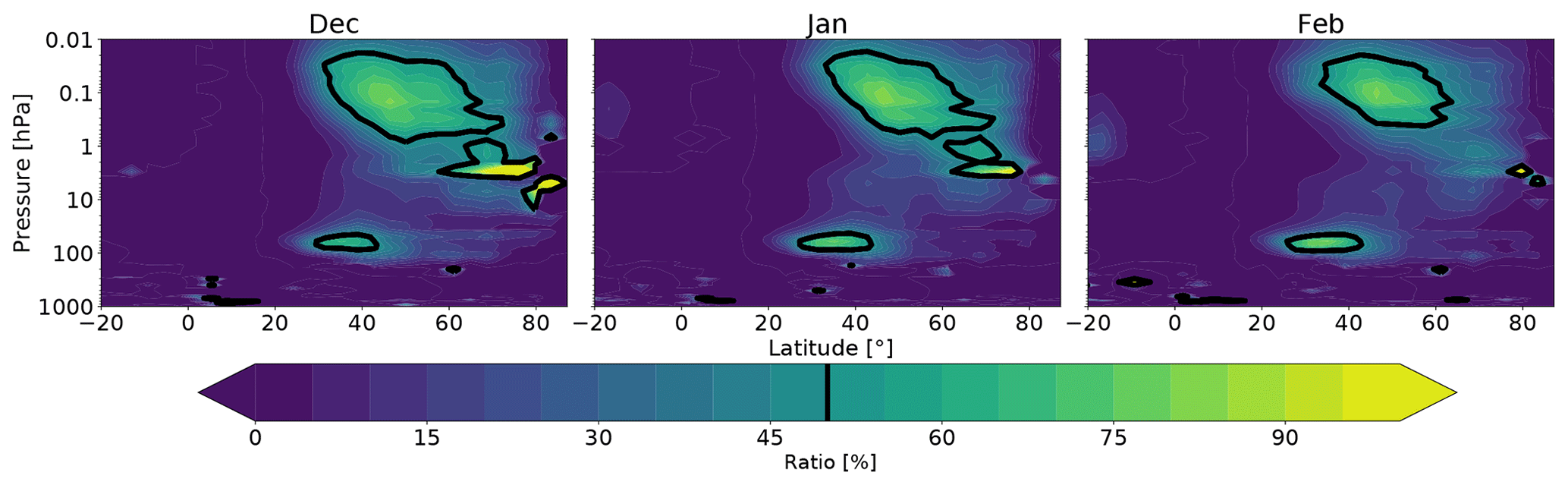
Figure 1 shows the boreal winter (DJF) average of the zonal-mean OGWD contribution to the total (OGWD + NGWD + resolved wave drag represented by Eliassen–Palm flux divergence – EPFD) zonal mean wave drag in the NH in CMAM-sd. Here two regions emerge in the middle atmosphere where the OGWD dominates the net drag, namely the lower mesosphere and the LS. In the lower mesosphere, OGWD controls most of the net drag between 40 and 75^∘ N in all months with the exception of the boreal summer months (not shown). In the LS between 25 and 50^∘ N, OGWD constitutes the majority of the net drag during boreal winter and adjacent spring and autumn months. The region of the LS OGWD maximum in the extratropics at 70 hPa starts at the upper flank of the subtropical jet and extends into the area of weak winds below the polar night jet. According to theoretical considerations postulated in Teixeira (2014) or following observational evidence from lidar measurements (Ehard et al., 2017), these areas, known as the valve layers (e.g., Kruse et al., 2016; Bramberger et al., 2017), are regions where weak or zero horizontal winds provide critical levels for OGWs. There, they break and deposit horizontal momentum. The dominance of the zonal mean OGWD forcing in the NH LS net drag emerges also as a robust feature in the free-running simulations with global (chemistry) climate models (including CMAM; Šácha et al., 2019; Okamoto et al., 2011; Dietmüller et al., 2018). In reanalyses, zonally averaged GWD constitutes about half of the net forcing in the LS (Albers and Birner, 2014; Abalos et al., 2015; Sato and Hirano, 2019).

Figure 1 Ratio of zonally averaged OGWD in zonal direction (units: %) to the total wave forcing (resolved waves represented by EPFD + OGWD + NGWD) for the climatological average of the period 1979-2010. The black contour represents 50 % contribution of OGWD. Adapted from Sect. 3 in Kuchar (2018).

The dominant OGWD in the LS at 70 hPa is mostly distributed into hotspots connected with regions of distinct topography. In our analysis, we focus on the hotspots highlighted by the colored boxes in Fig. 2. The amber, green and purple boxes represent the Himalayas (HI, 70–102.5^∘ E and 20–40^∘ N), West America (WA, 235–257.5^∘ E and 27.5–52^∘ N) and East Asia (EA, 110–145^∘ E and 30–48^∘ N) hotspots, respectively. The HI and WA hotspot areas have been defined based on the mountain range locations. The definition of the EA hotspot is not that straightforward as it corresponds to a geographical location of multiple mountain ranges. Several studies have reported the importance of the EA region as a “vertical communicator” from the troposphere into the stratosphere (e.g., Nakamura et al., 2013; Cohen and Boos, 2017; White et al., 2018). Strong OGW activity in the LS in this region has also been shown in observations. Šácha et al. (2015) have highlighted peak GW activity in the LS in a pronounced localized region corresponding to the EA hotspot as defined here. Moreover, Pisoft et al. (2018) showed that this region is unique because the background winds provide here a critical line for wave propagation in the LS.

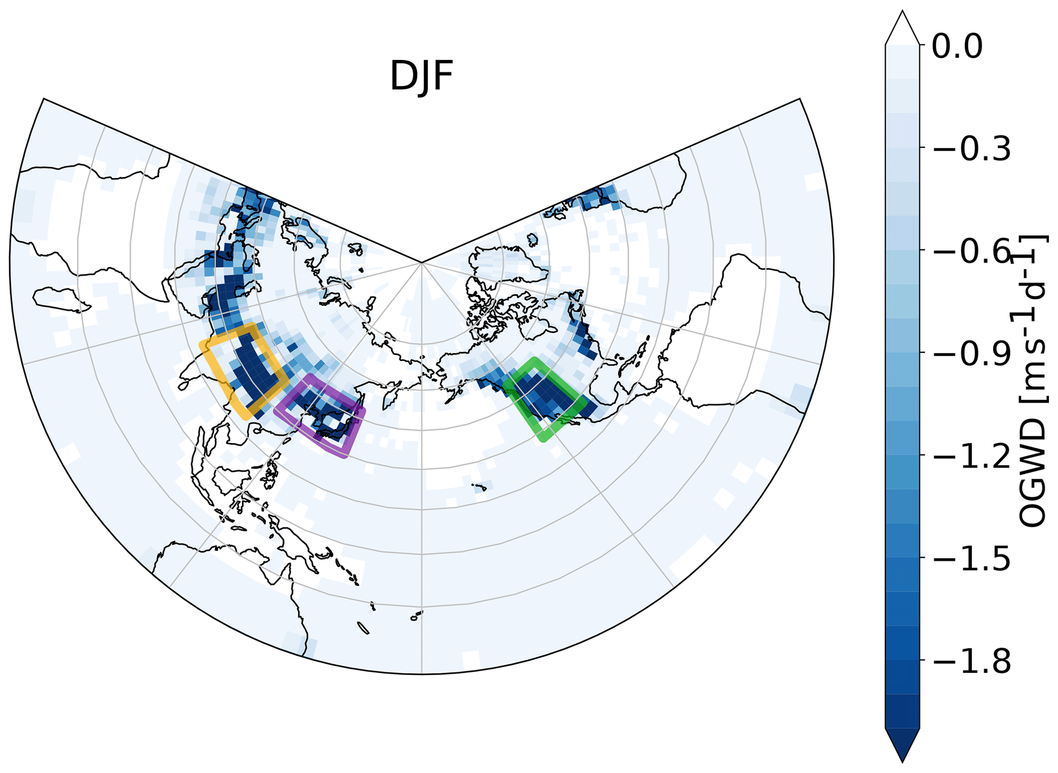
Figure 2 Boreal winter climatology of the zonal OGWD component (m s⁻¹ d⁻¹) at 70 hPa over the period 1979–2010. The amber, green and purple boxes represent the Himalayas (70–102.5^∘ E and 20–40^∘ N), West America (235–257.5^∘ E and 27.5–52^∘ N) and East Asia (110–145^∘ E and 30–48^∘ N) hotspots, respectively. Adapted from Sect. 3 in Kuchar (2018).

In order to analyze the CMAM-sd simulation with respect to the importance of asymmetrical GW forcing, we turn now to the analysis of these three hotspot regions. To create a representative OGWD time series for a particular hotspot, we area-weighted (using the cosine of the latitudes as weights) and averaged the OGWD at each grid point within the selected hotspots. With OGWD we refer here only to the zonal acceleration through OGWs. As shown in Fig. S1 in the Supplement comparing meridional and zonal components of OGWD at 70 hPa in our selected regions, the meridional component of OGWD can significantly contribute to the total drag from parameterized OGWs in CMAM-sd. However, as the dynamical role of the meridional acceleration is widely unknown (e.g., Šácha et al., 2016), we do not consider it in the analysis of the current paper but encourage its further investigation in future studies. For this type of analysis, we used daily mean values of the 6-hourly model data. The resulting OGWD time series for the three hotspot regions is shown in Fig. 3. The OGWD is generally small during summer and large during winter. In the parameterization the prevailing westward GWD is mainly determined by the near-surface wind speed and its direction relative to the orientation of the subgrid topography (McLandress et al., 2013; Šácha et al., 2018). During winter, many peak OGWD events can be seen in all hotspot time series.

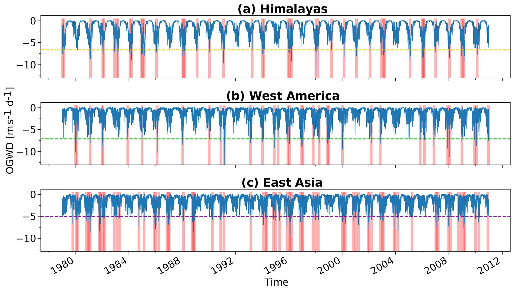
Figure 3 Area-weighted average of daily OGWD within the areas representing the Himalayas (a), West America (b) and East Asia (c). Peak events separated by 20-day timescale are highlighted by pink bars (see main text for explanation). Horizontal dashed lines show the OGWD threshold of the peak detection algorithm. For greater detail we refer the reader to the interactive figures in the Supplement. Adapted from Sect. 3 in Kuchar (2018).

To characterize the intermittency of (strong) OGWD events, we apply a peak-detection algorithm to detect peaks (local minima) that exceed immediate neighbors separated by more than 20 d. Only the peaks with amplitude beyond the normalized threshold are detected:

$$\begin{array}{}\text{(1)}& \mathrm{threshold}=\mathrm{0.55}(\min \mathrm{OGWD}-\max \mathrm{OGWD})+\max \mathrm{OGWD}.\end{array}$$

Here, the factor 0.55 is a free parameter to assess relatively strong events. The normalized threshold accounting for the time series range is different for each GW hotspot; i.e., it is −6.66 m s⁻¹ d⁻¹ for the Himalayas, −5.07 m s⁻¹ d⁻¹ for East Asia and −7.13 m s⁻¹ d⁻¹ for West America, respectively. Note that those threshold values represent the area-weighted average and even values 1 order of magnitude larger can be seen in individual grid points (see Sect. 3.2). The 20 d timescale was selected to be consistent with the definition of a simplified version of the World Meteorological Organization (WMO) criteria for SSW detection proposed by Charlton and Polvani (2007) using the reversal of the winds at 60^∘ N and 10 hPa and split and displacement SSW events employed in Seviour et al. (2013). The identification of strong OGWD events allows us to calculate composite anomalies of different variables by subtracting daily values from the monthly long-term climatology. The monthly climatology excludes months where SSW split and displacement events occurred according to the criteria of Seviour et al. (2013). The statistical significance and corresponding p values of the composites were derived through application of a bootstrap method based on 10 000 samples. The relative change of the particular variable was averaged according to the days preceding the identified peak events (lags from −10 to −1) and the days following the identified peak events (lags from +1 to +10).

3 Results

3.1 Evaluation of zonal mean GW diagnostics

We carry out comparisons of zonal mean GW parameterization outputs with observations to classify GW representation in CMAM-sd in relation to former validation efforts (Geller et al., 2013). A comparison of zonal mean absolute GW momentum fluxes from GRACILE and CMAM-sd is shown in Fig. 4. We analyze explicitly the sum of both GW fluxes (OGWs and NGWs), because it is impossible to derive pure OGW momentum fluxes from satellite observations. We restrict the analysis to boreal winter months in the lower and middle stratosphere, i.e., at 20 km and 30 km, respectively. These are the closest levels to the LS OGWD maxima in the NH extratropics (see Fig. 1) and the two lowest altitudes available from GRACILE for HIRDLS and SABER, respectively. Figure 4 shows that GW momentum fluxes in CMAM-sd largely overestimate the values from GRACILE between 30 and 60^∘ N in December and January at both levels. The shading represents climatological maxima or minima, which denotes the natural variability during the time periods used for averaging. In February, the modeled fluxes drop to much lower amplitudes at 30 km, which largely improves the agreement with the observations. However, the CMAM-sd fluxes in February still exceed those from observations by a factor of 2. Note that limb-sounder momentum flux estimates from HIRDLS and SABER are known to be systematically low-biased (e.g., Ern et al., 2004; Wright et al., 2015), which may be one of the reasons for such a significant overestimation as shown in Fig. 4. While the momentum flux distributions of GRACILE reveal maxima around 50^∘ N, the CMAM-sd fluxes show a latitudinal structure with multiple local maxima between 40 and 70^∘ N. At lower latitudes observations show larger and non-zero fluxes compared to the values produced in the CMAM-sd parameterizations, especially at 20 km.

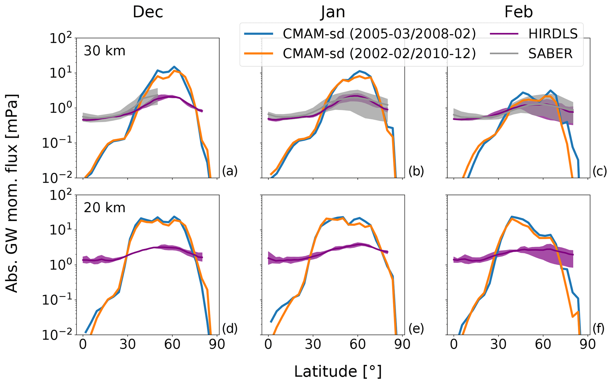
Figure 4 Climatologies for the absolute GW momentum fluxes (mPa) at 20 km (a–c) and 30 km (d–f) from CMAM-sd averaged over the HIRDLS period (March 2005–February 2008), over the longer period (February 2002–December 2010), respectively, and from SABER. The shading represents climatological maxima or minima adopted from the GRACILE dataset.

Comparison with Fig. 2 in Geller et al. (2013) reveals that CMAM-sd agrees well in terms of latitudinal GW variation but overestimates absolute GW momentum fluxes in the NH compared with other models. Geller et al. (2013) also documented in their Fig. 1 that absolute GW momentum fluxes from HIRDLS or SABER are larger during winter in the SH than in the NH. Furthermore, they show a similar overestimation of fluxes by models for January 2006 in the NH, while for July 2006 in the SH, models agree better with the observations. A comparison of the austral winter climatology of CMAM-sd momentum fluxes with GRACILE in the SH leads to the same conclusion (better agreement of magnitude), especially north of 60^∘ S (not shown). Those results underline the fact that the parametrization of OGWs in CMAM-sd is tuned to represent a missing drag in the SH (McLandress et al., 2012) resulting in the overestimation of the absolute GW momentum fluxes in the NH. We note that a similar effect of GW parameterizations has been recently documented for CESM1-WACCM4 (Garcia et al., 2017).

In Fig. 5 we show a comparison of the net zonal-mean OGWD (blue line) and NGWD (orange line) from CMAM-sd and reanalyses (JRA-55 – red line – and MERRA-2 – black lines) at 70 hPa (∼18 km) in the NH, i.e., the region of the LS OGWD maximum (see Fig. 1). In comparison with reanalyses, CMAM-sd overestimates the net GWD by about a factor of 2 from 30 to 70^∘ N. These are the latitudes where OGWD almost entirely determines the total GWD in CMAM-sd. However, when we add MERRA-2 assimilation analysis increments to the GWD tendency similarly to Scheffler and Pulido (2015), MERRA-2 still does not show as strong decelerations as CMAM-sd in the extratropical LS. This may stem from differences in OGWD parameterizations of MERRA-2, JRA-55 and CMAM-sd since the two-wave momentum flux representation in CMAM-sd leads to 30 %–50 % more GW momentum flux up into the middle stratosphere than the single-wave representation (used in MERRA reanalyses; McFarlane, 1987), depending on the pressure level and season (Scinocca and McFarlane, 2000). After accounting for the analysis increment, MERRA-2 (black dotted line) and JRA-55 (red line) agree remarkably well in terms of both amplitude and meridional distribution of the negative values of GWD, especially between 25 and 50^∘ N. Positive GWD values in MERRA-2 (black dotted line) at low and high latitudes can be interpreted as missing GWD from NGWs, which are typically launched with small amplitudes so that they deposit their momentum in the upper stratosphere and mesosphere (Kruse et al., 2016).

Figure 5 Climatology of parameterized zonally averaged OGWD (blue line) and NGWD (orange line) (m s⁻¹ d⁻¹) at 70 hPa in January averaged over the period 1980–2010. The black solid line represents the MERRA-2 tendency of eastward wind due to GWD and the black dotted line with the additional tendency of eastward wind from assimilation analysis, respectively. The red line represents the JRA-55 tendency of eastward wind due to GWD. Adapted from Sect. 3 in Kuchar (2018).

The climatological relative contribution of parameterized GWs to the resolved drag represented by the EPFD (see Eq. S4) agrees well between CMAM-sd and MERRA-2 and is slightly larger in JRA-55, albeit the GWD maximum (minimum of EPFD) being shifted to higher latitudes in CMAM-sd (see Fig. S2). This suggests that while GWD in reanalyses is smaller (Kruse et al., 2016), the resolved wave forcing may compensate the parameterized GWD (van Niekerk et al., 2018). In reanalyses the residual term of the zonal-mean momentum budget is still present in the LS (e.g., for JRA-55 see Fig. 2 in Martineau et al., 2016; Seviour et al., 2012, for ERA-Interim). NGWD is almost zero at 70 hPa in CMAM-sd, and the residual term coincides with the OGWD latitudinal maximum (see Fig. S3) between 30 and 40^∘ N, which may stem partly from missing NGWs at lower latitudes or underestimated OGWD (Seviour et al., 2012).

In summary, from the traditional zonal mean, monthly mean perspective we have shown that the OGW fluxes and drag in CMAM-sd are overestimated in the NH LS in comparison to observations and reanalyses, respectively. These biases have to be kept in mind in the following analysis and in the discussion of the results. In the next section we show that the OGW flux and drag cannot be fully described by the zonal mean quantities because they are strongly alternating in time and space.

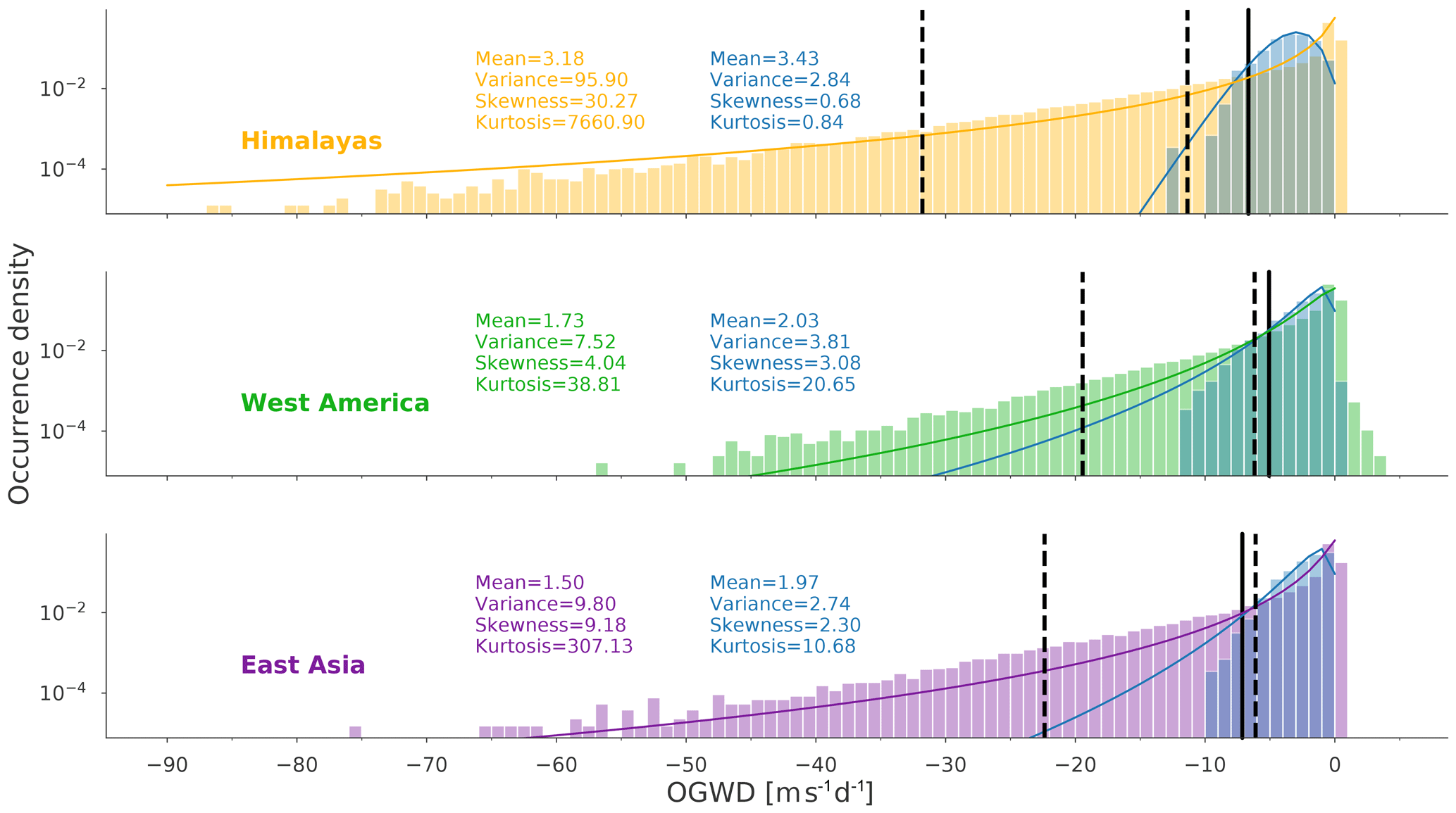
Figure 6 Daily OGWD distribution at 70 hPa during boreal winter within the Himalayas, West America and East Asia hotspot, respectively. Blue columns represent spatially averaged OGWD over the hotspot regions. Columns with different colors (amber for HI, green for WA and purple for EA) are unaveraged OGWD of all grid boxes within the hotspot regions, respectively. Vertical dashed lines show the value of the 10th and the 1st percentiles for the unaveraged OGWD. The vertical solid lines show the OGWD threshold of the peak detection algorithm (see Sect. 3.3). The corresponding fits of the log-normal distributions and their moments (mean, variance, skewness and kurtosis) are displayed as well. Note that the negative values of OGWD were used as positive values for fitting (and the originally positive part of the OGWD spectrum was not fitted).

3.2 Intermittency

The CMAM-sd OGWD spatial distribution is zonally asymmetric, which can be seen in Fig. 2 and in Šácha et al. (2018). In this section, we analyze the distribution of the OGWD magnitude in the three selected NH hotspots (HI, WA and EA). Figure 6 shows the probability density function (PDF) of the OGWD magnitude for the three hotspots at 70 hPa during boreal winter. The PDF is computed from the spatially averaged OGWD over the whole hotspot (blue columns) and from the unaveraged OGWD time series of all grid boxes within the hotspot location (amber for HI, green for WA and purple for EA). Dashed vertical lines show the value of the 10th and the 1st percentiles for the unaveraged times series, and the solid vertical line indicates a threshold OGWD value that is later in the article used to construct the composites of strong events for spatially averaged OGWD within the hotspots (see Sect. 3.3 below).

Figure 6 shows that the averaged OGWD values reach maxima around −10 m s⁻¹ d⁻¹. The PDF for HI follows a log-normal distribution, but the EA and WA hotspots do not reflect OGWD fitted values stronger than −10 m s⁻¹ d⁻¹ (see blue curves in Fig. 6, i.e., corresponding fits of log-normal distributions). In the spatially not averaged data we observe much broader tails of the PDF, and OGWD values reach up to −90 m s⁻¹ d⁻¹ in HI and −75 m s⁻¹ d⁻¹ in EA and WA. However, for WA, OGWD events larger than 50 m s⁻¹ d⁻¹ are rare in comparison to EA and especially HI. This is also reflected in the position of the 10th and 1st percentile, which have the largest value for the HI hotspot. The 10th percentile is at approximately −6 m s⁻¹ d⁻¹ for both EA and WA hotspots, but the 1st percentile is connected with a somewhat stronger OGWD for EA in comparison to WA (−19.5 m s⁻¹ d⁻¹). Note that for WA we find in addition some less frequent positive drags up to 5 m s⁻¹ d⁻¹ similarly to the averaged OGWD.

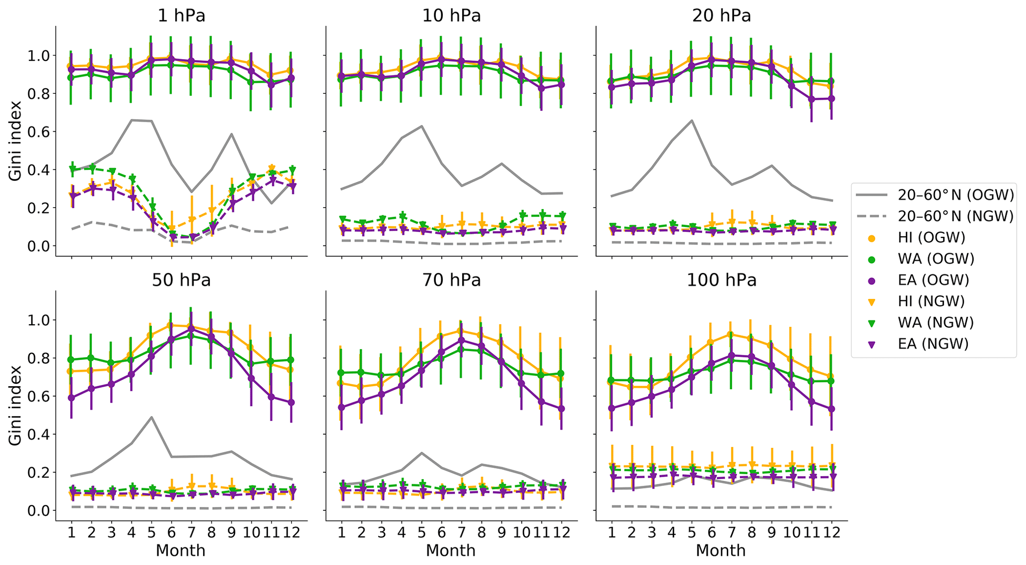
Figure 7 Spatial and annual variability of the Gini coefficient of GW momentum fluxes at 100, 70, 50, 20, 10 and 1 hPa within the Himalayas, West America and East Asia hotspots. Solid lines with circles and dashed lines with triangles represent OGWs and NGWs, respectively. Gray lines denote the Gini coefficient calculated from zonal mean between 20 and 60^∘ N. Error bars show the spatial standard deviation.

On the basis of recent observational studies (e.g., Hertzog et al., 2012; Wright et al., 2013), the intermittency of GWs has been increasingly acknowledged. Large GW events are known to be highly intermittent, which can be well quantified (Plougonven et al., 2013) by the so-called Gini coefficient (GC; Gini, 1912, the coefficient varies between 0, meaning a constant series without intermittency and 1, meaning maximum intermittency) usually calculated for GW momentum fluxes. For an exponential distribution GC is 0.5, and for a log-normal distribution the value is dependent on the standard deviation (Kendall and Stuart, 1977, p. 48):

$$\begin{array}{}\text{(2)}& \mathrm{GC}=\mathrm{erf}(\mathit{\sigma }/\mathrm{2})\equiv {\displaystyle \frac{\mathrm{2}}{\sqrt{\mathit{\pi }}}}\underset{\mathrm{0}}{\overset{\mathit{\sigma }/\mathrm{2}}{\int }}{\exp }^{-t^{\mathrm{2}}}\mathrm{d}t.\end{array}$$

The intermittency of OGW momentum fluxes in the atmosphere as well as of OGWD in the model is influenced by the sourcing processes as well as by the variability of the background flow during propagation. Figure 7 shows the annual cycle of GC for spatially averaged GW momentum fluxes over the hotspots (see Figs. S4–S11 for horizontal distributions of GC). In the upper to middle stratosphere (upper row in Fig. 7) the OGW fluxes are extremely intermittent with a weak annual cycle with maxima during boreal summer. This does not necessarily indicate strong OGWD in boreal summer as shown in Fig. 3, but it rather indicates that moderate OGWD occurs very sporadically and that the boreal summer climatological OGWD is weak. In the LS, GC of the OGWs is smaller in the boreal winter months for all hotspots. Still, OGWs in the LS can be considered as highly intermittent (minimal $\mathrm{GC}=\mathrm{0.5}\pm \mathrm{0.05}$). The three hotspot intermittencies of OGWD are comparable or slightly higher than estimated for OGW momentum fluxes from observations above regions with distinct topography ranging from 0.35 to 0.8 for the Antarctic Peninsula (Alexander et al., 2016; Jewtoukoff et al., 2015; Plougonven et al., 2013; Wright et al., 2013). Especially for OGWs in the upper stratosphere, the calculated GCs largely resemble the log-normal distribution estimate according to Eq. 2 (see Figs. S12 and S13 for GC estimated from log-normal distributions of OGW and NGW momentum fluxes, respectively). This is in agreement with the studies by Hertzog et al. (2012) and Plougonven et al. (2013), who found this relationship in balloon and spaceborne observations, and mesoscale numerical simulations. The intermittency of the hotspot regions is also clearly larger than the intermittency calculated from the NH mid-latitude (20–60^∘ N) zonal mean GW fluxes ranging from 0.1 to 0.4 in the LS (gray lines in Fig. 7). In other words, a significant amount of the intermittency is lost due to the zonal averaging of momentum fluxes. GC of the NH mid-latitude OGW fluxes shows the largest intermittency in spring and a secondary maximum in fall. This semiannual variation is larger with altitude and thus determined by the GW propagation conditions associated with the background atmosphere (Cao and Liu, 2016). During winter OGWs can permanently find favorable propagation conditions and act more continuously. Therefore OGW intermittency is reduced in winter when climatological OGWD is stronger and therefore more relevant in a traditional concept of stratospheric dynamics.

In the LS there are larger intermittency differences between the hotspots. During boreal winter, the lowest intermittency emerges for the EA hotspot. This can be connected with the fact that it consists of multiple mountain ranges with different orientations which may be favorable for more frequent fulfillment of conditions prone to launch freely propagating GWs and therefore resulting in lower intermittency compared to a single mountain range with uniform orientation. The intermittency of OGWD in the WA and HI remains high (minimally around 0.7) during the winter months. The annual cycle for WA is not as pronounced as for the other hotspots. GC in the LS slightly increases with altitude, suggesting that lower stratospheric background flow variability (critical line occurrence, Doppler shifting) plays only a minor role. The momentum flux intermittencies in the LS and at 850 hPa are comparable (see Fig. S14), pointing towards an important contribution of near-surface variability. A similar result has been derived for variability at longer timescales (Šácha et al., 2018). Only the EA hotspot reveals a weak annual cycle at 850 hPa suggesting that the annual cycle exposed for HI and WA in the stratospheric levels is determined by the background-flow variability.

The parameterized NGWD derived from spatially uniform fluxes at the launch level is also intermittent. Near the launch level in the LS (where NGWD is negligible) GC is about 0.1, but it increases with altitude and reaches 0.4 during boreal winter in the upper stratosphere (see dashed lines in Fig. 7). The low intermittency at lower altitudes is related to uniform momentum fluxes at the launch levels. Higher above larger NGW intermittency arises due to vertical propagation through variable background winds especially in boreal winter. Note that GC would be higher and show a more pronounced seasonal variability if the GW parameterization in CMAM-sd was source related.

3.3 Composite analysis

In the previous sections we demonstrated that the OGWD is a zonally asymmetric and intermittent forcing that dominates the total wave drag in the NH LS during the boreal winter. We propose a method for studying the OGWD influence by constructing strong-peak event OGWD composites of particular hotspots. To reduce the OGWD complexity we make the assumption that the OGWD inside a particular hotspot is homogeneous. Figures 6 and 7 showed that spatial averaging inside the hotspots changes the distribution (compare corresponding moments displayed in Fig. 6) as the information about the long tails of the distributions with strong (and apparently very localized) drag values of −15 m s⁻¹ d⁻¹ is lost, and also the approximation by the log-normal distribution no longer characterizes the spatially averaged OGWD distribution as good as the Weibull minimum extreme value distribution (see Fig. S15). On the other hand, the mean value of both distributions is approximately equally justifying the utilization of composites from spatially averaged OGWD for dynamical analysis. The magnitude of higher-order moments (especially kurtosis as a measure of the “tailedness” of the distributions) is another measure of the intermittency (Zel'Dovich et al., 1987; Mahrt, 1988). The spatially averaged OGWD represents still a highly intermittent forcing in the LS.

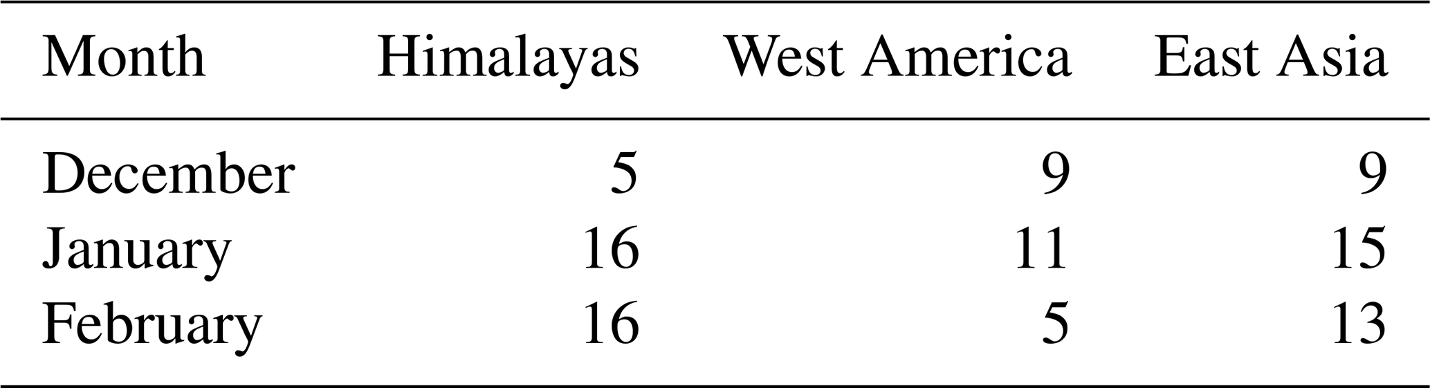
The number of days with detected peak events by the peak detection algorithm is shown in Table 1. For HI and WA the majority of detected strong OGWD events falls between November (December for HI) and March, for EA between September and May. Most of the events occur for all hotspots in January. To construct the composites we restrict the analysis to DJF, allowing us to assume a similar climatology for all peak events. Figure 8 shows the composites of the spatially averaged OGWD anomalies corresponding with strong OGWD events for each hotspot on the 20 d timescale. We note in passing that we have analyzed these composites also with a 30 d timescale yielding practically identical results (not shown).

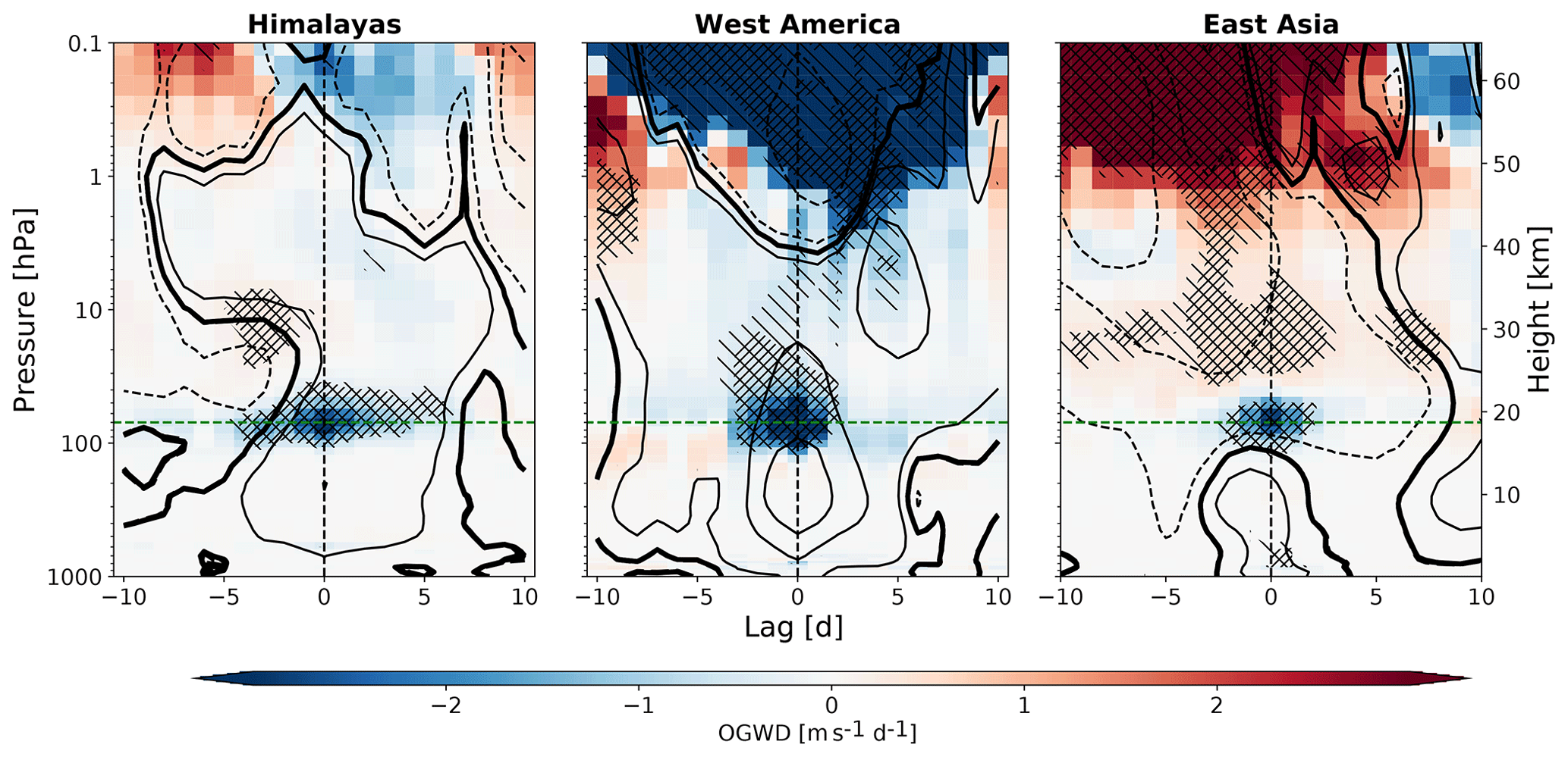
Figure 8 Composite anomalies of OGWD (m s⁻¹ d⁻¹) averaged at all lags within the selected hotspot areas (Himalayas, East Asia and West America) on the 20 d timescale. Green lines represent the composite level, i.e., 70 hPa. Hatching $\backslash \backslash \backslash \backslash$ and $////$ represents p values < 0.05 and <0.01, respectively. Dashed and solid contour lines represent negative and positive zonal wind anomalies with amplitudes {±1, ±5, ±8} m s⁻¹ within the selected hotspot, respectively. Solid bold line contours the zero-wind anomaly. Adapted from Sect. 3 in Kuchar (2018).

Table 1 Number of detected peak events per month for the three selected hotspot areas. DJF values are emphasized.

The composites of peak OGWD events within the hotspots naturally appear as statistically significant OGWD anomalies in the LS. The duration of the strong OGWD event differs slightly between the hotspots. For HI, OGWD anomalies are pronounced (smaller than −1 m s⁻¹ d⁻¹) for 5 d prior to the peak. For WA and EA, we find significant OGWD anomalies within 2 or 3 d prior to the peak (lag = 0). After the peak, strong OGWD anomalies occur up to +4 d for all hotspots. The vertical extent of the feature is similar in all three hotspots. For the HI and EA hotspots the OGWD anomaly reaches from about 100 to 40 hPa with a statistically robust peak at 70 hPa. The WA hotspot has a slightly larger vertical extent. The strong OGWD events are also connected with statistically significant OGWD anomalies at higher altitudes. Above about 1 hPa, anomalously strong and weak OGWDs for the WA and EA hotspot emerge, respectively. The OGWD anomalies in the upper stratosphere are negative but not significant for the HI hotspot. The enhanced OGWD results in a weakening of the westerlies in the mesosphere and is connected with strengthening of the westerlies throughout the stratosphere (see contour lines in Fig. 8) except for EA, where we found zonal wind weakening throughout the stratosphere. Absolute winds are usually eastward (positive) throughout the stratosphere and lower mesosphere except westward winds between 10 and 1 hPa for EA (not shown). This suggests that in the model the EA hotspot is connected with a critical level occurrence inhibiting further upward propagation of OGWs, while in the WA hotspot strong OGWD events are connected with strong momentum flux events. For the HI hotspot, the results are not conclusive due to the large variability of the strong OGWD events.

As we observe different anomalies above the hotspots between the upper stratosphere and the lower mesosphere (see Fig. 8), zonal-mean composites of OGWD reveal a common positive pattern corresponding to the positive zonal mean zonal wind anomalies. It indicates that the suppressed OGWD is connected with a weaker meridional residual circulation from lower to higher mesospheric latitudes. By the continuity equation, the weaker meridional transport is associated with weaker downward motion in polar latitudes which may result in a colder mesosphere (Zülicke et al., 2018). The positive OGWD anomalies reported here are similar to those reported in Albers and Birner (2014) and in Song and Chun (2016), i.e., suppressed in the regions of weak winds before the displacement SSWs. Hence, there are potential links between the illustrated OGW hotspot composites and middle atmosphere dynamics and transport. For example, the timing and the frequency of SSWs can be related to the GW forcing in the hotspots, and the upward propagation of GWs into the mesosphere can be hindered. This way, the hotspot composites indicate potentially different impacts on dynamics and transport in the stratosphere. Analyses of these connections, however, go beyond the scope of the current paper and will be conducted in a follow-up study.

4 Discussion and conclusions

This study analyses the characteristics of parameterized OGWD in CMAM-sd with focus on the NH LS. The CMAM-sd model output has been chosen for the analysis based on public availability of essential variables (OGW fluxes and drag) in 3D and necessarily high temporal resolution. The present study is therefore also meant to constitute an example of open science benefiting from publicly available 3D GW variables with high temporal resolution. The fact that CMAM-sd is nudged ensures that the meteorological situation is close to reality, particularly in the LS, and therefore makes comparisons with observations feasible. However, forcing the model dynamics also complicates the causal attribution of composite anomalies due to the two-way interplay between the OGW forcing and the circulation in the middle atmosphere. In this study, we do not consider this to be crucial, particularly, because the nudging is activated up to an altitude of 1 hPa only. We encourage modeling centers to provide the GW diagnostics in three dimensions and with at least daily sampling to access the GWD intermittency also for free-running simulations. This information may help to improve the validation of model GW fluxes with observations and consequent tuning of the drag strength.

Besides other known factors (e.g., neglection of horizontal propagation and directional absorption of GWs), different GW intermittencies can contribute to the discrepancies of GW fluxes and drags between models and observational estimates or induce completely different impacts on the model atmospheres for “correct” zonal mean GWD climatologies. While the downward control principle (Haynes et al., 1991) practiced in zonal mean is appropriate when studying momentum transfers by large-scale waves for which the approximation by zonally symmetric torques is reasonable, it may not be appropriate for studying atmospheric responses to momentum deposition associated with GWs (Shaw and Boos, 2012; Boos and Shaw, 2013).

We compared the zonal mean monthly mean OGWD and OGW momentum fluxes in the LS with reanalysis and observation-based data, respectively. This comparison showed that the CMAM-sd OGWD and the OGW momentum fluxes are almost 1 order of magnitude larger than in observations. These differences may be explained by the fact that the parameterization of OGWs is tuned to represent a missing drag in the SH resulting in the overestimation in the NH (McLandress et al., 2012). Using horizontal propagation and directional absorption of OGWs in the parametrization may bring the GWD in the middle latitudes closer to observations (Xu et al., 2017, 2018). On the other hand it should be considered that GW momentum fluxes as derived from satellite observations may be underestimated (Trinh et al., 2015; Ern et al., 2018). Still, the high bias in the NH emerges as a deficiency of current GW parameterizations in GCMs in pursuit of eliminating the missing GWD near 60^∘ S (McLandress et al., 2012), which is possibly associated with NGWs (Jewtoukoff et al., 2015).

The OGWD PDF can be approximated by a log-normal distribution. Within the selected hotspots (Himalayas, East Asia, West America) we can find extreme OGWD values exceeding −70 m s⁻¹ d⁻¹. After constructing one representative time series for each hotspot by spatial averaging, the long tails of the distribution are reduced and we observe drag magnitudes of up to about −15 m s⁻¹ d⁻¹. Based on the Gini coefficient, we show that the hotspot-averaged OGWD is highly intermittent and comparable with past observational studies (Alexander et al., 2016; Jewtoukoff et al., 2015; Plougonven et al., 2013; Wright et al., 2013). For all hotspots the intermittency is induced predominantly by the near-surface variability. However, the role of background flow variability in the LS also plays an important role, especially for EA, where near-surface momentum fluxes partly stipulate the annual cycle in the stratosphere.

Taking into account the spatiotemporal distribution of OGWD, we develop a method to study the impact of localized peak OGWD events in the three selected hotspot areas. The peak-detection method is based on locally strongly negative OGWD and therefore independent of the high bias outlined above. We construct composites of peak OGWD events at 70 hPa and apply the method to spatially averaged OGWD profiles connected with the particular hotspots to obtain information on duration and vertical structure of the strong OGWD events. This helps us to infer the nature of those events. The assumption of vertically propagating GWs applied in model parameterizations seems to be realistic in the LS (see Fig. 7 in Kalisch et al., 2014), which enhances confidence in our composites. One of the key results of our study is that LS peak OGW events can have opposing effects on the upper stratosphere and mesosphere depending on the hotspot region. Taking a zonal-mean perspective reveals that positive OGWD anomalies contribute to mesospheric cooling (Zülicke et al., 2018) when stratospheric winds weaken.

The analysis presented in this study constitutes a new method for studying the intermittency of OGWs, especially in hotspot regions, where the intermittency was shown to be large. Additionally, the composite analysis constitutes a new possibility to analyze the effect of the OGW hotspot regions on middle atmospheric dynamics, widening our understanding of the effects of GWs on dynamics and transport.