Intraseasonal variability of ocean surface wind waves in the western South Atlantic: the role of cyclones and the Pacific South American pattern

Extratropical cyclones are known to generate extreme significant wave height (swh) values at the ocean surface in the western South Atlantic (wSA), which are highly influenced by intraseasonal scales. This work aims to investigate the importance of intraseasonal timescales (30–180 d) in the regional climatology of waves and its atmospheric forcing. The variability is explained by analyzing the storm track modulation due to westerly winds. These winds present timescales and spatial patterns compatible with the intraseasonal component of the Pacific South American (PSA) patterns. The analyses are made using ECMWF’s ERA5 from 1979 to 2019 and a database of extratropical cyclones based on the same reanalysis. Empirical orthogonal function (EOF) analyses of the 10 m zonal wind and swh are used to assess the regime of westerlies and waves in the wSA. The EOF1 of the 10 m zonal wind (u₁₀) presented a core centered at 45^∘ W and 40^∘ S, while the EOF2 is represented by two cores organized into a seesaw pattern with a center between 30–40^∘ S and another to the south of 40^∘ S. Composites of cyclone genesis and track densities as well as swh fields were calculated based on the phases of both EOFs. In short, EOF phases presenting cores with a positive (negative) u₁₀ anomaly provide a favorable (unfavorable) environment for cyclone genesis and track densities and, therefore, positive (negative) swh anomalies. The modulation of the cyclone tracks is significant for extreme values of the swh. The spatial patterns of the EOFs of u₁₀ are physically and statistically consistent with 200 and 850 hPa geopotential height signals from the Pacific, indicating the importance of the remote influence of the PSA patterns over the wSA.

1 Introduction

Ocean surface gravity waves or wind waves (henceforth just called “waves”) are relevant for a number of socioeconomic activities over the coast. They may impact the safety of operations in ports, oil shelves and also present relevant coastal impacts related to erosion and building damage (de Andrade et al., 2019). These types of waves are generated by the wind, and, thus, extratropical cyclones (hereafter just “cyclones”) are responsible for driving most of the wave pattern at middle and high latitudes, generating extreme conditions in the western subtropical South Atlantic (wSA) (Fig. 1), where significant wave height (swh) may present values as high as 10 m (Gramcianinov et al., 2020c). The combination of waves and cyclones endangers the coastal population, and society can benefit from its improved understanding and predictability.

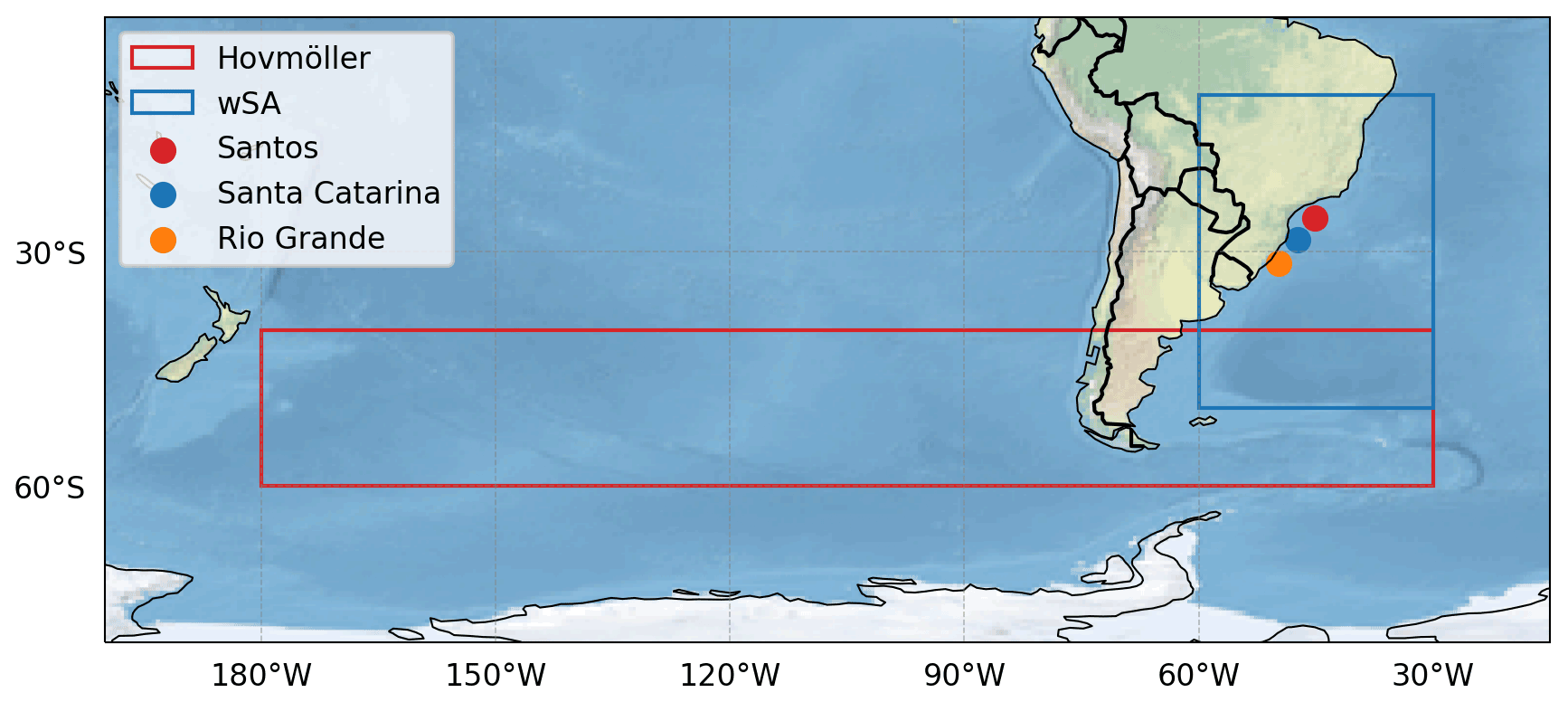
Figure 1 Domains and moorings used in this study: the wSA is the ocean area inside the blue rectangle; red rectangle shows the region used to calculate the Hovmöller diagrams (Sect. 3); circles show the approximate position of PNBOIA moorings used to evaluate the ERA5 swh results.

The wSA seasonal wave climatology description depicts a region with wave parameters influenced by easterlies from the South Atlantic subtropical high (SASH) and frequent (3 to 5 times per month) S/SE wind associated with cold fronts (Pianca et al., 2010). In the wSA, cold fronts are synoptic features associated with cyclones, which can generate extreme waves due to their strong winds (e.g., da Rocha et al., 2004; Campos et al., 2018; Gramcianinov et al., 2020c). There are three main cyclogenetic regions in the wSA coast: southeastern Brazil (SE-BR, 25^∘ S), Uruguay and southern Brazil (La Plata, 35^∘ S), and central Argentina (ARG, 45–55^∘ S) (Hoskins and Hodges, 2005; Reboita et al., 2010; Gramcianinov et al., 2019; Crespo et al., 2020). The presence of high cyclone genesis activity impacts directly the wave climatology in wSA, mainly from cyclones generated in the La Plata region (Campos et al., 2018; Gramcianinov et al., 2020c, 2021).

Apart from the seasonal scales, a possible source of predictability of the waves could be related to the atmospheric interannual and intraseasonal variability. For instance, the North Atlantic Oscillation interannual variability is relevant in the modulation of significant wave height (swh) in the North Atlantic (Dodet et al., 2010). In the South Atlantic, Pereira and Klumb-Oliveira (2015) observed a significant but weak El Niño–Southern Oscillation (ENSO) signal in the swh in wSA. However, so far global studies of waves showed no significant relation between climate indices such as the ENSO or the Southern Annular Mode (SAM) and the waves over the wSA, when the interannual component is considered (Godoi et al., 2020; Godoi and Torres Júnior, 2020; Reguero et al., 2015). On the other hand, there is a rise of evidence of modulation in intraseasonal timescales of the wave fields by atmospheric processes (e.g., Godoi and Torres Júnior, 2020; Srinivas et al., 2020). As an example, the Boreal Summer Intra-Seasonal Oscillation (BSISO) in the tropical Indian Ocean is part of the summer monsoon and influences the surface winds, consequently modulating the swh anomalies over its different phases (Srinivas et al., 2020). Over the Pacific, Atlantic and Indian oceans, Godoi et al. (2020) found significant dependences between the increase in austral summer swh anomalies and different ENSO–MJO (Madden–Julian Oscillation) phase combinations.

In the South Atlantic, there are a few eligible atmospheric intraseasonal patterns that may influence the wave field. The Pacific South American patterns (PSA), for instance, are wave trains in the geopotential height anomaly fields, which propagate from eastern Australia to Argentina (Mo, 2000). PSA is originally known as interannual processes identified by two modes of the geopotential height: PSA1, with a dominant spectral peak between 36–40 months; and PSA2, with a dominant peak between 24–26 months. According to Mo and Paegle (2001), PSA1 would be associated with the low-frequency component of ENSO, while PSA2 would be related to a quasi-biennial modulation of ENSO. More recently O'Kane et al. (2016, 2017) have given a new perspective of PSA, showing evidence of the strong influence of synoptic-to-intraseasonal timescales. These authors performed a study to analyze the persistence of SH variability modes in a multiscale approach and found that PSA2 and another mode (fifth mode) are not well correlated with ENSO (O'Kane et al., 2017), as suggested before. O'Kane et al. (2016) found a quasi-stationary pattern in the South Pacific, which presents the same patterns as the PSA modes but on synoptic-to-intraseasonal timescales. This signal has been associated with blocking in the Pacific and Atlantic and highlights the need for further investigation of PSA influences over South America, not only in terms of low-frequency but also considering intraseasonal timescales.

The importance of intermediate timescales in South America (SA) was also reported by recent works which identified the existence of an intraseasonal modulation of the atmospheric circulation, precipitation and marine heatwaves (e.g., Paegle et al., 2000; Rodrigues et al., 2019). The SA dominant precipitation pattern in the summer is a dipole with centers of action over the South Atlantic convergence zone (SACZ) and the subtropical plains (e.g., Paegle et al., 2000; Liebmann et al., 2004). Paegle et al. (2000) showed intraseasonal oscillatory modes with periods of 36–40 and 22–28 d, both related to the MJO. However, the last was also influenced by PSA-like wave trains propagating from the midlatitude Pacific and turning equatorward as it crosses the Andes Mountains, which is supported by Liebmann et al. (2004). The observed change in precipitation is driven by circulation change: the low-level jet is enhanced or suppressed depending on the dipole phase, which may also lead to a cyclonic disturbance development near the 30–35^∘ S region (Vera et al., 2002; Gramcianinov et al., 2019). In fact, patterns similar to PSA are strictly related to synoptic system propagation, being associated not only with precipitation, but also with blocking, drought and marine heatwaves (Rodrigues and Woollings, 2017; Rodrigues et al., 2019). The modulation of cyclones could have major implications for ocean waves.

Therefore, the PSA can be considered a potential source of predictability in the wSA, influencing some meteo-oceanography variables in the intraseasonal scale. For this reason, we hypothesize this variability mode also interferes in the wave field over the region. In this way, the questions that arise are the following:

1. Is the intraseasonal signal significant over the wSA regarding the wave field?

2. If yes, what is the local forcing associated with this variability?

3. Can this intraseasonal variability be linked to PSA? Since the surface wind field forces the wave field, it is used here as a proxy of the atmospheric variability, associated with the geopotential height at 200 hPa (Z₂₀₀) and 800 hPa (Z₈₅₀). In addition, once cyclones play an important role in wave generation, cyclone track analysis is also applied.

The document continues with Sect. 2 describing the datasets and methods used in this work. Section 3 presents the results, showing the wind and wave variability in the intraseasonal timescale, the role of the modulation of the cyclones as regional forcing, and the analysis regarding PSA signal. The discussion is provided in Sect. 4 followed by the conclusion in Sect. 5.

2 Data and methods

2.1 Datasets

The ERA5 reanalysis is a detailed reconstruction of the global atmosphere, land surface and ocean waves. It is the fifth generation of reanalysis produced by the European Centre for Medium-Range Weather Forecast (ECMWF; Hersbach et al., 2020) and made available through the Copernicus Climate Change Service (Copernicus Climate Change Service, 2017). This reanalysis is produced using 4D-Var data assimilation in ECMWF'S Integrated Forecast System (IFS), which is coupled with the wave model WAM (WAMDI Group, 1988). The atmospheric variables present 31 km (0.28125^∘) spatial resolution, while wave parameters are in 0.36^∘ resolution. Both atmospheric and wave data are available in hourly output from 1979 to the present (3-month delay). The data used in this study cover the period from 1979 to 2019, with the atmospheric variable on a $\mathrm{0.25}{}^{\circ }\times \mathrm{0.25}{}^{\circ }$ grid and the wave parameters on a $\mathrm{0.5}{}^{\circ }\times \mathrm{0.5}{}^{\circ }$ grid. An overview of the main characteristics of ERA5 can be found in Hersbach et al. (2019, 2020).

ERA5 presents an improved fit for winds, temperature, and humidity in the troposphere as well as for the ocean wave height when compared to its predecessor, the ERA-Interim reanalysis (Hersbach et al., 2020). Belmonte Rivas and Stoffelen (2019) showed that ERA5 surface winds present an improvement of 20 % relative to ERA-Interim, using Advanced Scatterometer (ASCAT) observations as verification, which is especially important since surface wind misrepresentation is one of the major sources of wind-wave modeling biases (e.g., Campos et al., 2018). Moreover, ERA5 is able to represent the Atlantic storm track distribution and characteristics, e.g., cyclone intensity (Gramcianinov et al., 2020a).

Regarding the wave field, Takbash and Young (2020) found that the reanalysis has a good agreement in mean parameters and a global centennial wave height magnitude and spatial distribution similar to the ones estimated by altimeter and buoy. Despite that, coastal regions are more susceptible to model systematic errors (biases) as a result of the simplification of physical processes associated with shallow and intermediate water interactions and the inherited wind surface biases (e.g., Campos et al., 2018). Because of that, an evaluation of the ERA5 wave parameters was performed using buoy data. For that, we used an array of moored buoys, which are part of the Global Ocean Observing System and Brazil’s national buoy program (PNBOIA; see Pereira et al., 2017, for more details) and have measured meteo-oceanographic parameters since 2011. Among the entire data collection, three sites have better temporal availability: São Paulo, Santa Catarina and Rio Grande buoys. The evaluation showed a high skill of ERA5 swh between 2011 and 2018, both for wave magnitude and variability. The results are presented in detail in the Appendix A (Fig. A1).

2.2 Cyclone identification and tracking

To analyze the influence of the synoptic systems in the ocean surface wave variability, we used the “Atlantic extratropical cyclone tracks in 41 years of ERA5 and CFSR/CFSv2 databases” (Gramcianinov et al., 2020b), which consists of a database containing cyclone track information from 1979 to 2019 for all Atlantic Ocean. The extratropical cyclones were tracked using the TRACK algorithm (Hodges, 1994, 1995) following the method developed by Hoskins and Hodges (2002, 2005). The minimum duration and displacement of the cyclones are 24 h and 1000 km, and only cyclones that spent a part of their life cycle within South Atlantic extratropical latitudes (85–25^∘ S, 75^∘ W–20^∘ E) are considered. More information regarding the database method and evaluation is available in Gramcianinov et al. (2020a).

Cyclone genesis and track spatial statistics, i.e., density, were computed using TRACK utilities applying the spherical kernel estimator method (Hodges, 1996). Cyclogenesis density was built by using the position (latitude, longitude) where each cyclone was first detected by the algorithm, i.e., the first time step of each track, while the track density considered the entire cyclone tracks. The significance for the differences of the cyclones spatial distributions between empirical orthogonal function (EOF)/principal-component time series (PC) positive and negative phases (see Sect. 3.1) was calculated using Monte Carlo test (Hodges, 2008) with 1000 samples of the set of tracks for each phase.

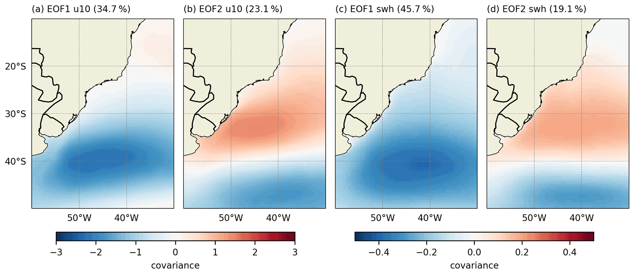
Figure 2 EOFs of filtered anomalies of (a, b) 10 m zonal wind (u₁₀) and (c, d) significant wave height (swh) calculated on the wSA. The percentages represent the explained variance of each mode.

2.3 EOF and wavelet analysis

Anomalies and filtered anomalies of swh, meridional 10 m wind (v₁₀), and zonal 10 m wind (u₁₀) were calculated from the ERA5 dataset. The anomaly computations are obtained by subtracting the mean daily climatology from the original fields, while in the filtered results, anomalies were subjected to a Lanczos bandpass time filter with cutoff periods of 30 and 185 d. The selection of the cutoff period is based on the relevance of the intraseasonal variability indicated by the regional precipitation, marine heatwaves, and PSA (O'Kane et al., 2017; Rodrigues et al., 2019) and based on the results in Sect. 3.1.

We use empirical orthogonal function (EOF) analysis (Dawson, 2016) to reduce the dimensionality of the data and decompose both anomaly and filtered fields over the wSA (Fig. 1). Removing the variability associated with periods smaller than 30 d in filtered anomaly fields avoided the inclusion of atmospheric meso- and synoptic-scale propagating systems (e.g., cyclones and fronts). The first and second modes (EOF1, EOF2) produced by the analysis were selected, and the results in Sect. 3 show they are physically meaningful.

EOF analysis is usually applied over basin-size domains and captures features that correspond to large-scale processes. In the Southern Hemisphere, for instance, the spatial signal of the Southern Annular Mode is present in the EOF of both seasonal swh (Hemer et al., 2010) and geopotential height fields (Mo, 2000). On the other hand, these large domains tend to separate the variability of large-scale features in a given mode, which may attenuate (or even not show) the signature of a given regional process, such as the lobes in EOF maps in Fig. 2 in O'Kane et al. (2017). For this reason, we chose to restrict the EOF analysis to the wSA. Moreover, a wavelet analysis (Torrence and Compo, 1998) with a bias rectification (Liu et al., 2007) is used to identify relevant periods in the PCs of the EOFs.

Table 1 Correlation matrix between the EOFs of $u_{\mathrm{10}}/v_{\mathrm{10}}$ and swh filtered anomalies at lag 0.

3 Results

3.1 Wave and wind spatiotemporal variability

Figure 2 shows the first and second modes of the EOF of u₁₀ and swh filtered anomaly fields. The EOF1 of u₁₀ and swh (Fig. 2a and c) presents similar spatial patterns with cores centered at 45^∘ W and 40^∘ S. The EOF1 of the u₁₀ corresponds to 34.7 % of the explained variance, and the monopole is associated with strengthening/weakening of the wind anomalies. This variability may appear as an intensification, weakening or even reversal of the total u₁₀ over the region. Similarly, the EOF1 of the swh (Fig. 2c) is also organized into a monopole, which retains 45.7 % of the total explained variance. The EOF2 of the u₁₀ and swh (Fig. 2b and d) consists of a dipole with centers between 30–40^∘ S and to the south of 40^∘ S and presents an explained variance of 23.1 % and 19.1 %, respectively. The spatial patterns in the EOFs of the anomalies are omitted since they are very similar to the EOFs of filtered anomalies. The PC of the EOF1 of the anomaly and filtered anomalies of u₁₀ and swh is presented in Fig. 3. These results exemplify the period from 2004 to 2008 and show the filtered fields retain a signal similar to the EOF of the anomaly fields. Results associated with the second mode of the EOFs of u₁₀ and swh (not shown) present similar patterns to the first mode.

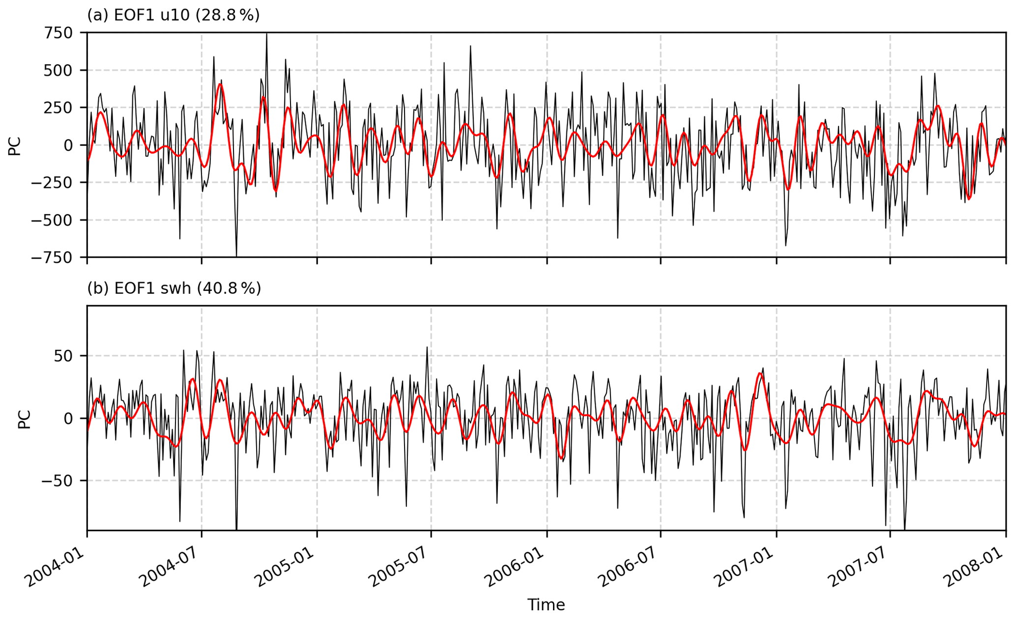
Figure 3 PC of the (a) EOF1 of u₁₀ and (b) EOF1 of the swh. Black lines represent the PC of the anomaly fields, and red lines represent the PC of filtered anomaly fields. The percentages represent the explained variance of EOF modes considering the anomalies fields.

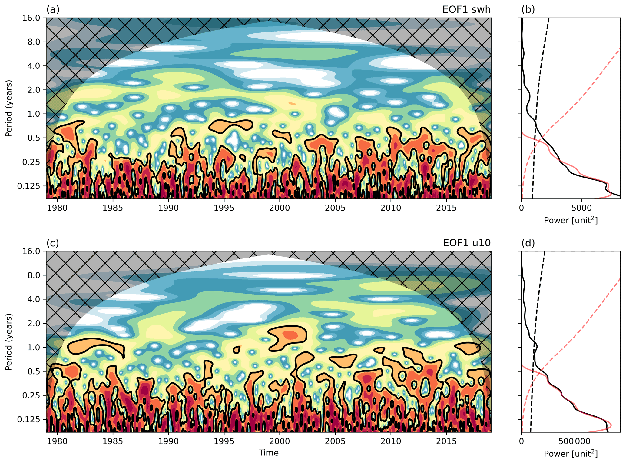
Figure 4 Wavelet power spectrum of the EOF1 of swh anomaly (a) and u₁₀ anomaly (b); the black contours represent the 95 % confidence level. Global wavelet spectrum of swh (c) and u₁₀ (d) for the anomaly fields (black) and filtered anomaly fields (red). Dashed lines represent the 95 % confidence level considering a red noise based on a univariate lag-1 autoregressive model.

The values in the PC correlation matrix of the filtered u₁₀, v₁₀ and swh (Table 1) show correlation coefficients greater than 0.50 between the EOF1 of u₁₀ and swh and also for EOF2, while the correlation between the EOF1 (EOF2) of u₁₀ and EOF2 (EOF1) of swh presents correlation values of 0.40 (0.21). Correlations values lower than 0.4 were not analyzed, which was the case of the correlation coefficients between EOFs of v₁₀ and swh. The correlation values (highlighted in the table) indicate a direct intensification (weakening) of winds associated with greater (smaller) values of the swh, which are further evaluated in Sect. 3.3. The phase composites of u₁₀ and swh of the corresponding EOF modes are included in Appendix C.

Figure 4 shows the wavelet power spectrum and global power spectrum of the PC considering the EOF1 of u₁₀ and v₁₀. Both cases present significant values (p<0.05) only for the periods (T) between 1 and 6 months. Within this period band, the global wavelet spectra of filtered and unfiltered PCs of the EOFs present almost identical values. The analysis shows that in the western subtropical South Atlantic, the intraseasonal variability of u₁₀ and swh presents a significant signal, with the major peak at approximately 40 d. The results of the EOF2 in both u₁₀ and v₁₀ present similar results (not shown). Differences within the 35 to 180 d period in the global wavelet spectrum plot may be justified by the different inputs in the EOF analysis, but the similarity of the PCs in Fig. 2 and the EOFs (not shown) indicates the filtered results are reliable.

In the following sections, the intraseasonal relationship between the variability of swh, cyclone genesis and track densities is studied using composites of wave and wind fields based on EOF phases of u₁₀ and swh. We define phase A (B) periods when the PC values are greater (smaller) than 1 SD (standard deviation). These time series have physical meaning only when interpreted in conjunction with the spatial patterns of the EOFs (Fig. 2). For instance, phase A (B) corresponds to positive (negative) values in the time series (Fig. 5a), and the phase combination with the spatial patterns of the EOFs (Fig. 2) generates reconstructed fields with negative (positive) values (not shown), which correspond to the composite fields (Fig. 5b and c).

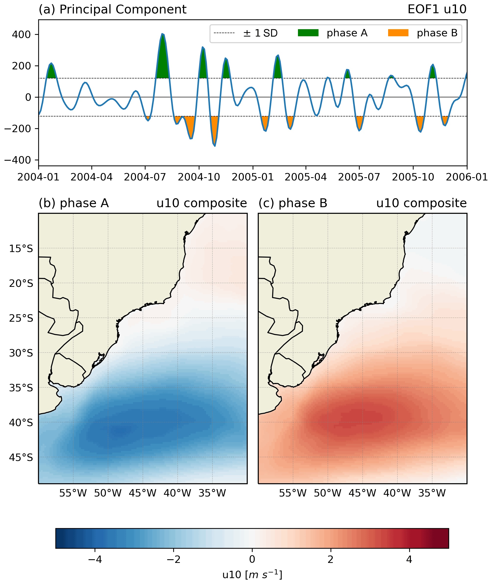
Figure 5 Time series of the EOF1 of (a) swh. Phase A (B) denotes periods when the time series presents values greater than (less than) +1 (−1) standard deviation. The composites are the average value of swh anomaly during (b) phase A and (c) phase B.

3.2 Cyclone genesis and track densities

The genesis and track density differences between u₁₀ EOFs phases (A minus B) are shown in Fig. 6, where regions with significant values are indicated by black dots. The track and genesis density for u₁₀ EOF1 can be found in Appendix B (Fig. B1), where it is possible to evaluate the spatial patterns of density in order to understand the differences discussed in this section. In Fig. 6, the spatial pattern of the track density differences is represented by a zonal tripole in the EOF1 of u₁₀, which distinguishes the regions over high, middle and subtropical latitudes, including the coastal area between Uruguay and southern Brazil. The track density differences show that phase B of EOF1/PC retains the main South Atlantic storm track between 40 and 55^∘ S, as reported in the literature (e.g., Hoskins and Hodges, 2005), resulting in fewer cyclones around Antarctica in a pattern similar to the one reported to the negative SAM phase (Reboita et al., 2015). In phase A, the opposite occurs, and the main storm track is shifted southward, resulting in fewer cyclones in middle latitudes. However, in these conditions, a secondary storm track emerges around 35^∘ S. The cyclogenesis density differences reinforce this pattern, presenting in phase B (A) less (more) genesis activity at the Antarctic Peninsula and more (less) activity between 40 and 55^∘ S, both in the ARG genesis region and the oceanic portion. The La Plata genesis region is enhanced in phase A, supporting the positive track density response at subtropical latitudes.

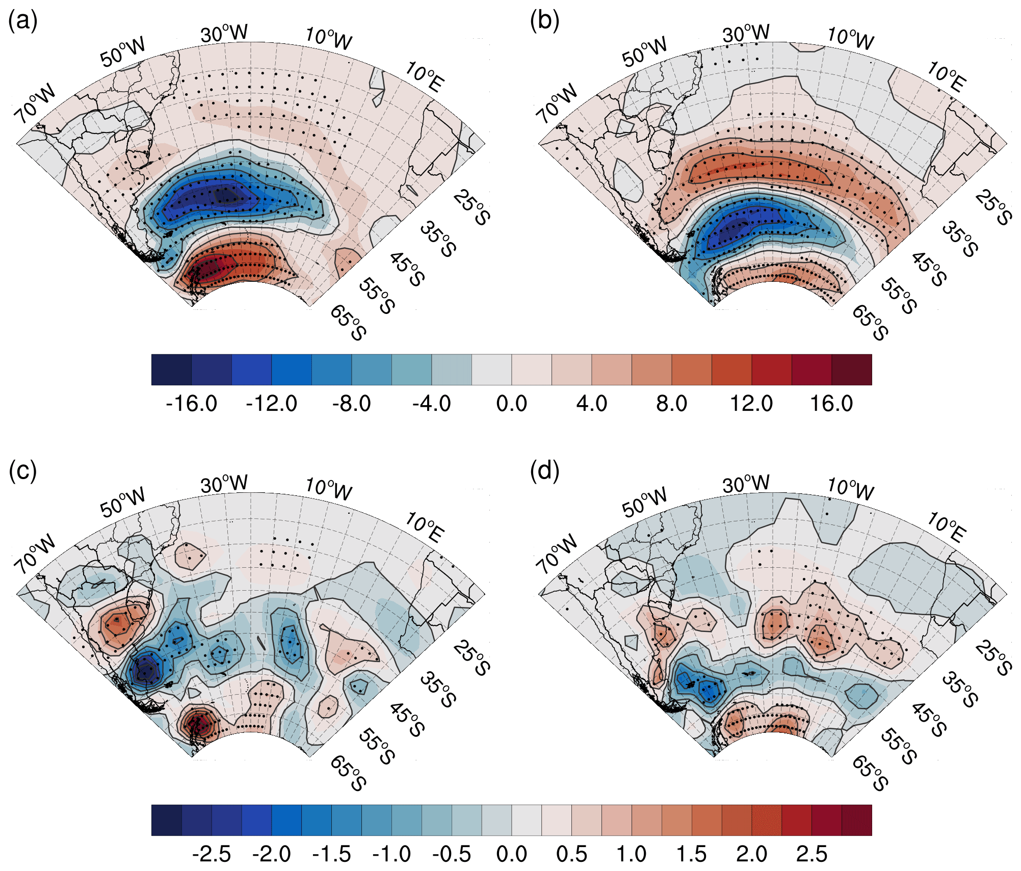
Figure 6 Cyclone (a, b) track and (c, d) genesis density differences between phases A and B of (a, c) EOF1 and (b, d) EOF2 of u₁₀. Differences are calculated using phases A minus B and are also contoured by 5 density unit intervals for the track and 0.5 for the genesis. The black dots indicate where the difference is significant within a 95 % confidence level. Density unit is the system per year per area, where area is in 10⁶ km² (∼5^∘ spherical cap).

The track density differences for EOF2 of u₁₀ also reveal a zonal tripole, with narrower zonal bands when compared to EOF1 tracks (Fig. 6b). In phase A (B), the cyclone activity presents a positive (negative) signal between 30–40^∘ S and 60–70^∘ S and a negative (positive) signal between 40–60^∘ S. By the genesis density, it is possible to see that genesis in La Plata and the northern ARG region is enhanced in phase A, as well in the Antarctic Peninsula. The genesis signal is mainly at the oceanic area adjacent to the southern Brazilian and Uruguayan coasts, which separates the traditional ARG genesis region into two, with the northern portion being active during phase A and the southern portion being active in phase B. The behavior observed in genesis and track densities can be interpreted as a direct consequence of the EOF2 pattern once it shows an enhancing (weakening) of westerlies at 35^∘ S (45^∘ S) in phase A, affecting baroclinic wave development for the same reason explained for EOF1. In both cases, the coupling between track densities and zonal wind anomalies is consistent with positive baroclinic feedback (Robinson, 2000), which shows that the mean flow modifications by baroclinic eddies, i.e., cyclones, reinforce the low-level baroclinicity.

The density differences based on the EOFs of swh revealed patterns similar to the u₁₀ case (Appendix B, Fig. B2). The storm track differences also present a tripole pattern as a consequence of the large-scale wind, similarly to Fig. 6. However, these swh-related fields are slightly weaker when compared to the u₁₀ case. This weaker response occurs because the swh is integrated by the local (wind–sea) and remote wave (swell) signal (Young, 1999; Chen et al., 2002). Strong winds associated with the cyclones contribute directly to the local generation and development of wind–sea, reflecting the observed similarities between Figs. 6 and B2. On the other hand, the remote wave signal – the swell – consists of propagating waves generated elsewhere (Alves, 2006; Ardhuin et al., 2009). In other words, the wind and wave fields are partially coupled through wind–sea, which explains the weaker signal in Fig. B2. Also, a meridional shift of a few degrees between the track composites in Figs. 6 and B2 is present. This shift can be explained by the generation mechanisms of waves within the asymmetric structure of extratropical cyclones. The fully developed sea state presents higher swh and takes place in the downwind end of the fetch (e.g., Ardhuin and Orfila, 2018), which is usually located northwest from the cyclone center in the wSA (Gramcianinov et al., 2021).

3.3 Waves composites

Significant changes in the wave fields are known to occur in higher percentiles, as in cases associated with extreme events (Young et al., 2011). For this reason the composite calculations are based on a percentile approach. Figures 7 and 8 present the differences between the composites of the swh 75th percentile on phases A and B of the EOFs of u₁₀ to ensure the EOF results represent real physical wind–sea interaction. The significance of the differences was calculated within the 95 % interval and determined by a bootstrap hypothesis test for the median of differences with 1000 realizations.

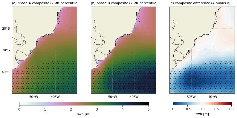
Figure 7 Composites (75th percentile) of swh calculated using phases (a) A and (b) B of the EOF1 of u₁₀ and (c) difference between the composites. The black dots represent the areas where the difference between phases is within a 95 % confidence level.

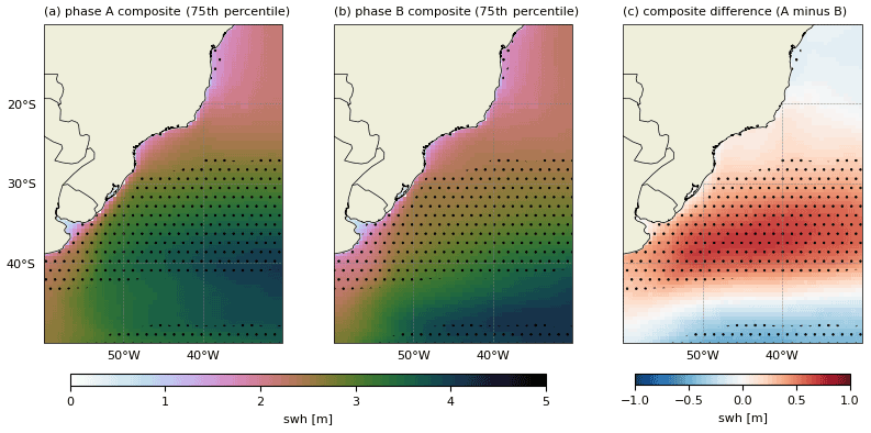
Figure 8 Composites (75th percentile) of swh calculated using phases (a) A and (b) B of the EOF2 of u₁₀ and (c) difference between the composites. The black dots represent areas where the difference between phases is within a 95 % confidence level.

The swh composite difference shows that phase A (phase B) in the EOF1 of u₁₀ is linked to negative (positive) anomalies in the swh fields southward of 35^∘ S (Fig. 7). The difference computed for the phases of the EOF2 of u₁₀ exhibits a seesaw pattern (Fig. 8), with positive (negative) values reflecting on the intensity of the wave anomalies in phase A (B). It is important to note that the composite differences are significant in a narrow area close to the central Brazilian coast (15–20^∘ S), which presents positive wave anomalies during phase A of u₁₀ (EOF1). Also, the differences related to the EOF2 of u₁₀ show the 75th percentile of the swh is relevant from northern Argentina towards the southern Brazilian coast. The signal in the extreme-wave composites follows the wind and wave behavior in each phase of EOFs discussed in the last section, given the similarity observed in Figs. 2, 7 and 8. However, the SW–NE orientation of the anomalies is more evident in the extreme composites, which indicates the dominant orientation the wave generation fetches in the wSA (e.g., Campos et al., 2018; Gramcianinov et al., 2021).

The relevance of the EOFs in the swh fields is further illustrated in Fig. 9, where composites of swh fields are determined from high-wave events (HWEs) and the percentage corresponding to the significant height of wind–sea (shws) is presented. We define HWEs as events where swh values at a point in the south Brazilian bight (SBB; magenta point) exceed a 3 m threshold while occurring concomitantly with at least one active cyclone at the selected domain (i.e., wSA). These composites are also built according to the different phases of u₁₀ EOF modes.

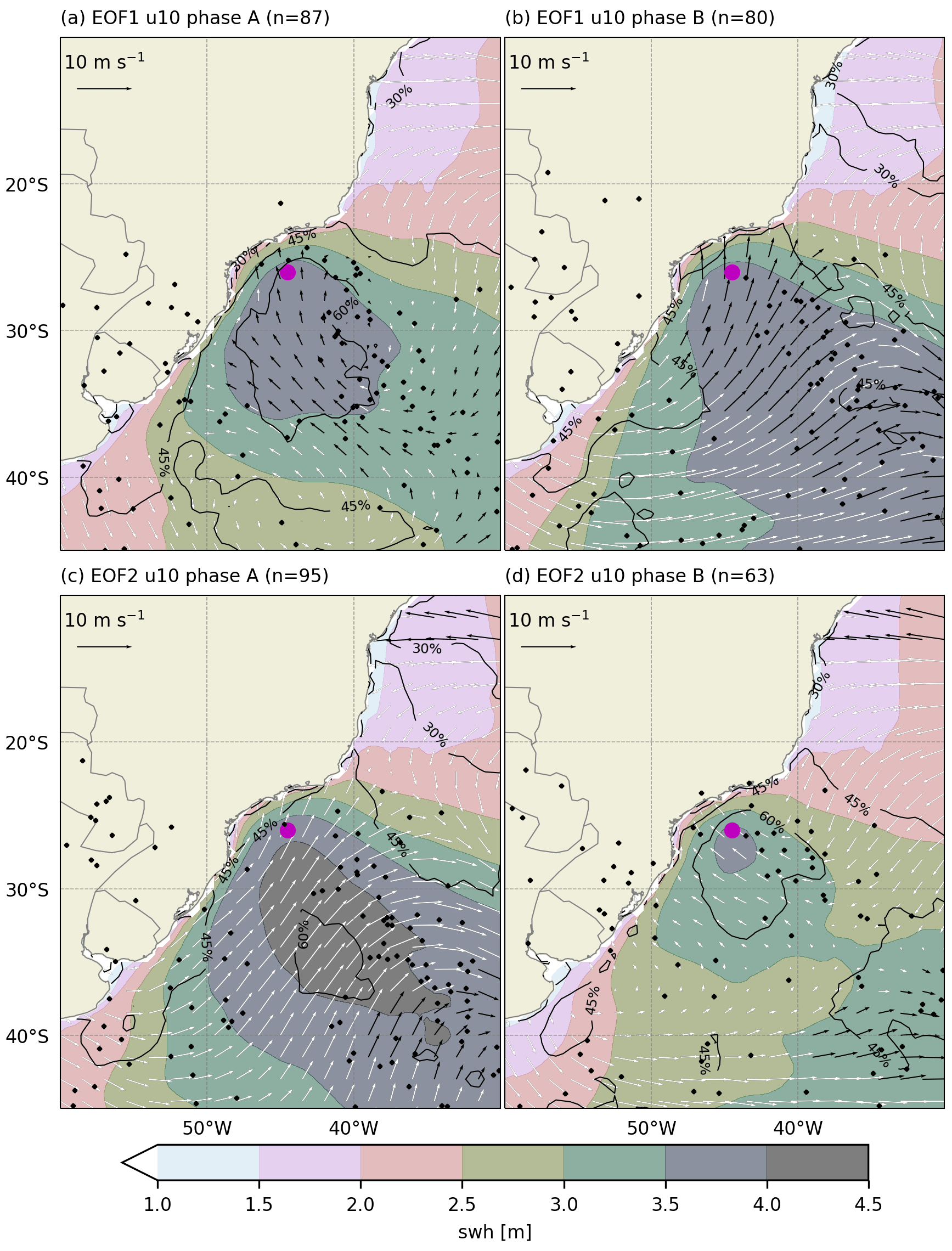
Figure 9 Composite of the total swh (shaded) for the high-wave occurrence in the SBB (purple dot; 30^∘ S, 45^∘ W) in the phases (a, c) A and (b, d) B for (a, b) EOF1 and (c, d) EOF2. The shws is shown as a percentage from the swh in contour lines, and the 10 m wind is indicated by the vector fields. White vectors are areas where the differences of swh between phases of a given mode are within the 95 % confidence level.

A similar number of HWEs (n∼80) was identified during phases A and B of the EOF1 of u₁₀ (Fig. 9a and b). The maximum mean swh (>3.5 m) in phase A is centered at approximately 30^∘ S and 45^∘ W, in the SBB region, with 60 % of these events associated with the shws. In phase B, high mean swh values are more distributed within the domain, following an NW–SE orientation, from the SBB region to the SE domain's boundary. Over the domain, the shws corresponds to 40 %–50 % of the swh. Both phases present a similar spatial distribution of cyclone centers, which are most often positioned to the southeast of the SBB, but cyclones are scattered also to the south and southwest of the SBB region. The effect of the wind composites shows the wind fields resembling a cyclone centered at 30^∘ S and 38^∘ W during phase A, whereas a trough-like pattern indicates a cyclonic circulation (smoothed by the composite) eastward from SBB in phase B.

In the composites of phases A and B of the EOF2 of u₁₀ (Fig. 9c and d), 95 and 63 HWEs were identified, respectively. Phase A is associated with a larger HWE number and also presents cyclones that occur mainly to the southeast but also to the southwest of the SBB. In this phase, swh values range from 3.5 to 4.5 m in a band oriented NW–SE from the SBB, where the shws corresponds to 60 % of the swh. The lower number of HWEs in phase B agrees with general lower swh values presented in the composite, with shws percentage corresponding to 40 %–50 % of the total swh. In this phase, the exception occurs over the SBB region, where the swh values range from 3.0 to 4.0 m and the percentage of shws is approximately 60 % of the swh. Here, the trough in the wind vectors is present in phase A, while a regional cyclonic wind pattern is centered near 25^∘ S and 42^∘ W in phase B.

Composites of transient-related events are often noisy since the cyclone’s position and associated features (e.g., cold and warm fronts) are mobile. For this reason, the wind patterns in Fig. 9 do not present a closed cyclonic circulation, but a trough instead. It is also possible to see cyclone–anticyclone (trough–ridge) pairs with different orientations, positions and magnitudes. This happens due to the rich variety of atmospheric patterns associated with extreme waves in the wSA (da Rocha et al., 2004; Solari and Alonso, 2017; Gramcianinov et al., 2020c). In fact, Gramcianinov et al. (2020c) showed that the presence and relative position of the anticyclone to the cyclone may contribute to the extreme-wave event generation by enlarging the fetch and increasing the wind speed.

3.4 Evaluation of remote signal

Up to this point, we have shown that the EOFs of u₁₀ within the intraseasonal band are significant for the variability of cyclones and waves in the wSA, especially regarding the extreme-wave events. The remaining question is the following: is this variability pattern a part of a larger organized system? Over the wSA, the spatial patterns revealed by the EOFs of u₁₀ are similar to features of the PSA found using EOFs of the geopotential height (Irving and Simmonds, 2016). There is little agreement as to what EOFs of the geopotential height represent to the sub- and extratropical environment between the South Pacific and South Atlantic – some associate it to SAM and PSA (Ding et al., 2012), and others relate it to an eastward-propagating wave train that may be connected to MJO influence on the western South Pacific (Paegle et al., 2000; Liebmann et al., 2004; Irving and Simmonds, 2016). In the present study, correlation analysis at lag 0 between the PCs (monthly averages) and monthly SAM index (Marshall, 2003) yields values smaller than 0.1, indicating SAM is not relevant regionally. Hence, we concentrate our analysis on the PSA modes. Here, we will not consider the effect of MJO, since its influence is observed only during austral summer (e.g., Liebmann et al., 2004; Rodrigues and Woollings, 2017). Following the discussion and results presented by O'Kane et al. (2017), except in the summer, the subtropical jet works as a barrier to waves propagating from the tropics (e.g., Hoskins and Ambrizzi, 1993; Ambrizzi and Hoskins, 1997), reducing the influence of MJO in the SH extratropics. Restricting the analysis to a unique season would reduce the sample size and eliminate seasons where the cyclones and ocean surface waves are more severe in the region (e.g., Pianca et al., 2010; Gramcianinov et al., 2020c).

PSA modes evaluated by EOFs in the South Pacific and South Atlantic domains require multiple EOF modes (geopotential height, for instance) to depict the wave train signal in the atmosphere that extends from the central South Pacific to the South Atlantic (O'Kane et al., 2017; Irving and Simmonds, 2016). In contrast with the usual approach of using the geopotential height fields, the evaluation of the signal that propagates from the South Pacific into the wSA is made using Hovmöller diagrams. These diagrams do not separate the variability in different modes but provide valuable insights into the associated variability that are difficult to interpret using the EOF approach.

The PSA patterns occur across the South Pacific and South Atlantic domains, but the analysis of EOF in such a large domain would interfere and smooth the variability signal observed in the wSA. To evaluate the spatial distribution of the PSA patterns, usually observed in the Z₂₀₀ and Z₈₅₀ fields, we used composites during the different phases of the EOF of u₁₀.

Figure 10 illustrates a wave-like spatial signal in both geopotential height fields, which extends from 150^∘ W in the South Pacific to 20^∘ W in the western South Atlantic. The composites of Z₂₀₀ and Z₈₅₀ based on phase A of EOF1 of u₁₀ present multiple cores between 40 and 60^∘ S, alternating positive and negative values with an opposed signal to phase B. The stronger signal in Z₂₀₀ and Z₈₅₀ occurs in the South Atlantic in both phases and overlaps with the monopole observed in the EOF1 of u₁₀ (Fig. 2a) southward of 40^∘ S. The second most intense core extends from the Amundsen Sea in Antarctica (120–90^∘ W) towards the western coast of South America at 40^∘ S.

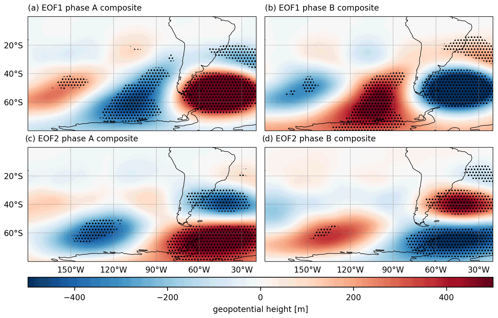
Figure 10 Composite of the geopotential height anomaly at 200 hPa (shaded) for the u₁₀ EOF1 in phase (a) A and (b) B, as well as EOF2 in phase (c) A and (d) B. Black dots denote where the signal is significant within the 95 % confidence level.

In both phases of the EOF2 of u₁₀ an alternating pattern is also present in the Z₂₀₀ and Z₈₅₀ composite fields. Phase A (B) presents a core with local maximum (minimum) in geopotential height fields on the South Pacific northward of the region (150–120^∘ W) between the Ross Sea and the Amundsen Sea. Over the South Atlantic, there are two main cores with a meridional distribution, with opposite signals between the phases. The first is located southward of 60^∘ S, and the second is centered at 40^∘ S, between the dipole pattern presented in the EOF2 of u₁₀ (Fig. 2b).

Considering that single EOF mode analyses are inappropriate for the evaluation of propagating signals, we used Hovmöller diagrams in the assessment of the PSA wave train propagation in the Z₈₅₀ and Z₂₀₀ filtered fields (30–185 d). The Hovmöller diagrams, presented in Fig. 11, are calculated in the area (meridional average) indicated in Fig. 1 and show patterns of variability from the period in between 1988 and 1996. The time interval choice is arbitrary and aims only to exemplify the signal propagation between the Pacific and South Atlantic domains. The Hovmöller diagram of Z₂₀₀ shows a complex pattern of intraseasonal variability, where part of the signal propagates eastward over time and shows wave-like features, such as the presence of an anomalous trough and ridge system, i.e., sequential positive and negative values. Thin green dashed lines in Fig. 11 exemplify positive signals in between 180 and 90^∘ W propagating towards 30^∘ W. These signals take up to 4 months to cross the South Pacific domain. Other features can be noted as westward-propagating signals (thick green dotted lines), revealing that not all intraseasonal variability in wSA is necessarily connected with the eastward-propagating features.

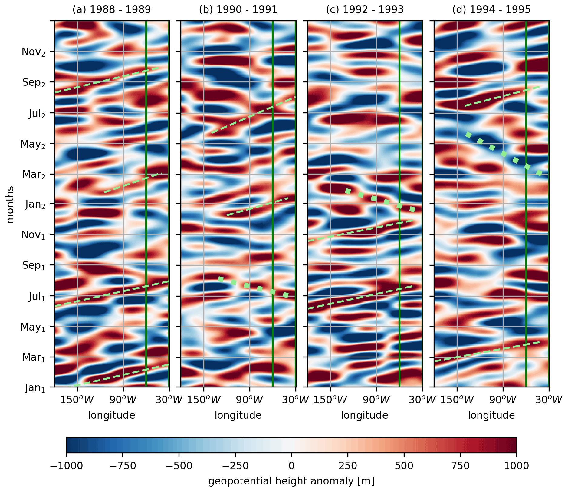
Figure 11 Hovmöller diagram of the filtered Z₂₀₀ anomaly signal from 1988 to 1995 and retains the variability within 30–185 d with a Lanczos bandpass filter. The green line indicates the longitudes corresponding to the wSA. The subscript 1 (2) in the month labels corresponds to the first (second) year indicated in the title of each panel.

4 Discussion

4.1 Intraseasonal variability in wSA

The frequency spectrum showed the relevance of the intraseasonal frequency in the u₁₀ over the wSA (Fig. 4). In the surface wind field, the pattern represented by EOFs may correspond to the westerlies' intensity and meridional variability forced by the midlatitude upper-level jet changes (e.g., Hare, 1960). The EOF1 of u₁₀ represents the strengthening (weakening) of the westerly wind belt around 30 and 45^∘ S in phase A (B). In this way, phase A of EOF1 of u₁₀ is associated with lower swh values, which also consists of periods with a less active storm track in the South Atlantic located between 40 and 55^∘ S (Fig. 6a). On the other hand, the intensification of the surface winds, observed in phase B, may play a role in the strengthening of baroclinic wave growth, as long as it reflects directly to the upper-level jet and baroclinicity (Hoskins and Ambrizzi, 1993; Ambrizzi and Hoskins, 1997). In this situation, more frequent and more intense cyclones are expected to develop in the region, thus representing a more efficient wave generation mechanisms. The EOF2 patterns, representing a meridional shift of the westerly wind and its effect on the cyclone patterns and wave fields, are analogous to the EOF1 explanation. Over different phases of the EOF2 of u₁₀, there is an enhancement (weakening) of the cyclone activity between 30–40^∘ S (Fig. 10b) in phase A (B) of the EOF2 of u₁₀, which leads to an increase (decrease) in swh values in the northern zonal band of the seesaw pattern represented in Fig. 2d. This is evidenced by both EOF2 of u₁₀ and swh, which exhibit an approximate superposition of the dipole structures (Fig. 2b and d). In this way, positive (negative) anomalies of u₁₀ linked with the EOF modes are associated with increases (decreases) in the swh anomaly fields. This relation is also reinforced by the positive correlation values computed for the PCs (Table 1) The same pattern is observed in the composites considering the 75th percentiles of the swh (Figs. 5 and 8). However, the percentile approach allowed a further view of how the intraseasonal modes interfere in the extreme waves. The changes in swh reach up to 1 m, which is a high value from the extreme analysis perspective. These patterns are important as they impact relevant economic areas in South America located at the central/southern coast of Brazil and the northern coasts of Argentina, Uruguay.

4.2 Impacts on regional extreme waves

The composite analysis described above provides a general view of the processes, but in order to have a more in-depth idea of the events in the wSA and include the cyclone information as part of the analysis, we evaluate the composites of high-wave events (HWEs) (Fig. 9). The selected region of this analysis lies purposely outside of areas with significant differences, which shows the area of influence of the EOFs of u₁₀ is not restricted to the significant areas represented in Figs. 7 and 8.

Cyclone tracks associated with the EOF1 of u₁₀ are mainly concentrated to the south of 40^∘ S. As a consequence the swh in the southern region is more affected by a given phase, despite the similar HWEs in both phases. In phase A we see high swh values concentrated over the SBB region due to the increase in genesis in La Plata (Fig. 7) but for cyclones with a small spatial range, i.e., short tracks (Fig. 6a). On the other hand, phase B presents an enhanced cyclonic activity between 40 and 55^∘ S, associated with the increase in genesis in the ARG region (Fig. 6d). This cyclone behavior justifies the spread swh pattern in phase B composites (Fig. 9b), once its contribution to the wave field in the region is also linked to its variable spatial scale (1500–2000 km radius) and swell propagation. In fact, the shws percentages in the composites show that the remote effect in the total wave field is larger in phase B than in A.

The EOF2 of u₁₀ presents a larger number of HWEs during phase A, and this is a consequence of the higher genesis and track densities between 35–45^∘ S. In phase B, more cyclones are generated southward of 45^∘ S, which lead to lower and less intense HWEs. However, a small region over the SE Brazilian coast (30^∘ S) presents more genesis (negative values in Fig. 6d), indicating a wind forcing source close to SBB. The cyclones generated in SE-BR are usually weaker and short-time systems, which can generate HWEs but not as frequently as the La Plata region (Gramcianinov et al., 2020c). Therefore, the swh composites are still presenting relatively high shws percentages, although the swh values are lower than those presented in the composite of phase A. One can note that the proximity of an active cyclogenesis region influences directly the percentage of shws relative to the total swh. However, the percentage never crossed the 60 % value, revealing a high influence of remote forcing in the SE Brazilian coast wave extremes.

Gramcianinov et al. (2020c) evaluated extratropical cyclone environments in the wSA and found three situations where extreme waves are generated:

1. west/southwestward of the cyclone center, behind the cold front;

2. north/northwestward of the cyclone center, ahead of the cold front; and

3. eastward of the cyclone center, along the warm front.

The most commonly observed case in the composites is situation 1, which is identifiable by the amount of cyclone centers placed to the east of the reference point (SBB) and the trough in the mean wind field. Situations 2 and 3 are more difficult to identify but are likely to be associated with the cyclone centers over the ocean occurring to the south and southwest of SBB, as well as over land.

4.3 South Pacific forcing

The composites of the geopotential height fields for different phases of u₁₀ EOFs show a wave train coming from South Pacific midlatitudes to wSA, similar to PSA as described in the multiscale approach of O'Kane et al. (2017). The intraseasonal signal over wSA is consistent with the features presented in the Hovmöller diagrams (Fig. 11), where the PC of the EOF1 (2) of u₁₀ presents an approximate linear response to the mean time series of the Z₂₀₀ (u₁₀) (Fig. 11). The area used to calculate the time series of Z₂₀₀ does not overlap completely with the wSA box, but it captures the monopole of the EOF1 of u₁₀ and the southern core of the dipole of the EOF2 of u₁₀. Eastward propagating from the South Pacific signals organized into wave train features.

The key point of the Hovmöller diagrams is to show these eastward-propagating systems can appear at some occasions in the South Pacific to the west of the 90^∘ W meridian months before reaching the wSA. The MJO variability is known to contribute to austral summer synoptic features over South America such as the South Atlantic convergence zone and atmospheric blocking (e.g., Liebmann et al., 2004; Rodrigues and Woollings, 2017) and could force part of the eastward-propagating signals in the Hovmöller diagrams with the origin to the west of 18^∘ W. Moreover, other eastward-propagating systems are present and start in between 160 and 90^∘ W. These cases may arise as the PSA modes are associated with local disturbances and the internal waveguide dynamics over midlatitudes (O'Kane et al., 2017). As discussed by O'Kane et al. (2017), apart from the summer, the subtropical jet reflects and breaks stationary Rossby waves from tropical sources, as shown by the ray-tracing theory (Ambrizzi et al., 1995; Li et al., 2015). In this way, the PSA pattern in the intraseasonal frequency consists of stationary Rossby waves generated by the subtropical and polar jets' internal instabilities, with little evidence for sustained equatorial tropical sources. Since the connection between the observed PSA pattern and EOF modes of u₁₀ exists, these results indicate these wave-propagating regimes impact cyclone genesis and track, as well as the associated wave fields, especially regarding the extreme waves.

5 Conclusions

This work aimed to investigate the existence and effects of the intraseasonal variability in the wave field over the wSA. To accomplish this goal, we established three main questions. (1) Is the intraseasonal signal significant over the wSA regarding wave field? (2) What are the local drivers associated with this variability? (3) Can this intraseasonal variability be linked to PSA? Regarding the first question, we found evidence of significant variability of the wave field in the wSA in intraseasonal timescales, with a dominant period of 38 d. This variability occurs in response to changes in intensity and position of the westerlies within the domain. The strength and shifts of the surface winds also lead to a modulation of cyclone tracks and genesis, which is strictly related to wave generation in wSA. In fact, the analysis of high percentile composites in each mode variability showed that the extreme-wave climatology is highly impacted by the intraseasonal scale, presenting variations up to 1 m of swh. This finding is relevant since the wSA is an economically active area, with many oil platforms and active ship routes. Such naval structures and activities demand high-quality forecasts and metocean analysis, which can benefit from the inclusion of more reliable intraseasonal timescale processes.

According to past studies that analyzed other variables (e.g., precipitation, sea surface temperature), one of the sources of intraseasonal variability in South America is the PSA (O'Kane et al., 2017). The MJO influence is also documented (Liebmann et al., 2004; Rodrigues and Woollings, 2017); however, its effects are usually observed in the summer. Guided by the findings of O'Kane et al. (2017), we considered that PSA patterns in intraseasonal scales during other seasons are led by internal variability of the subtropical and polar jets, excluding the influence of tropical convection and consequently MJO. We analyzed the wave train pattern present in the geopotential height at middle and upper levels and found a significant link between them and the intraseasonal variability modes presented for wave and wind field EOFs in the wSA domain. In our results, the signal of the wave train propagation from the South Pacific to the wSA occurs mainly eastward within 3 and 6 months. Also, we found a less frequent westward-propagating signal, which, although interesting, does not represent the PSA pattern.

Although we focused on the impact of the intraseasonal variability on the wave field, our analysis was restricted to wave height. In this way, it would be valuable to understand the impact of these intermediate timescales on other wave parameters, such as peak period, mean wave direction and others. Further investigations about the conditions that allow the propagation of this intraseasonal signal from the Pacific to Atlantic seem to be valuable, given the large controversy regarding PSA timescales and sources.

Appendix A

The validation of ERA5 swh results in the wSA with PNBOIA results is summarized in Fig. A1. The buoys present measurements between 2012 and 2019, and the swh values present high skill (>0.85) (Willmott, 1981), which is also confirmed by high correlations and a comparable standard ratio between model results and measurements. This validation suggests ERA5 is skillful in simulating the wave variability and consequently the associated surface wind patterns.

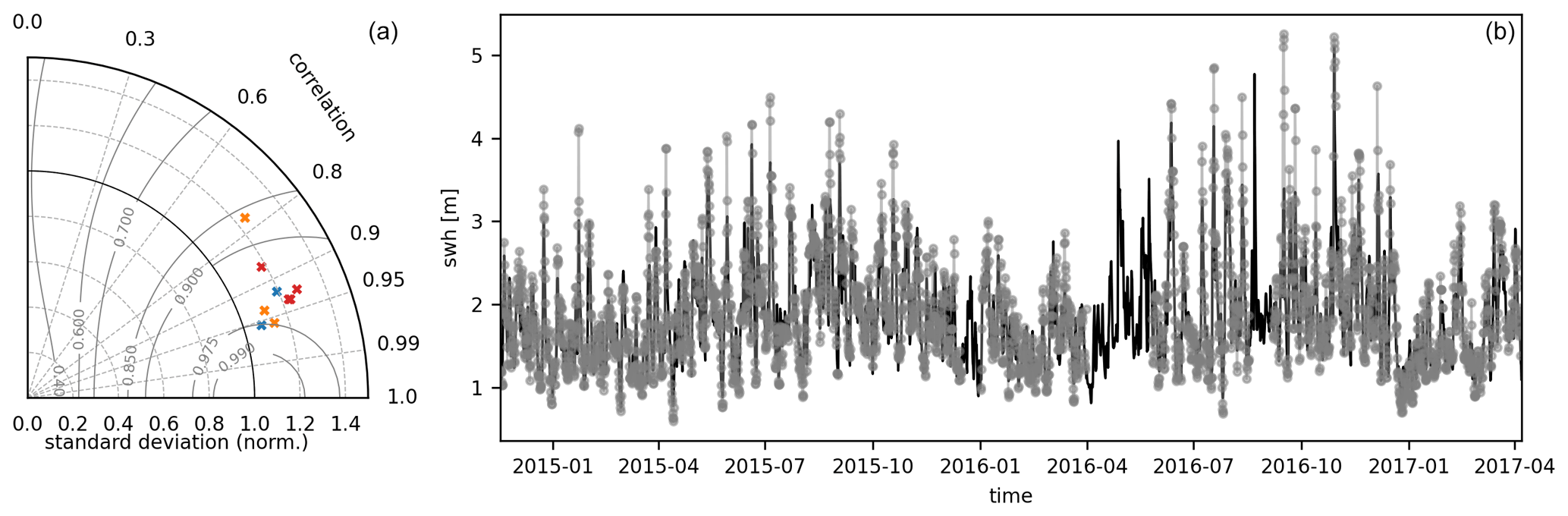
Figure A1 The Taylor diagram (a) summarizes the validation of ERA5 swh results with PNBOIA measurements using the results in the interval between 2012–2019. The markers represent different moorings at Santos (red), Santa Catarina (blue), and Rio Grande (orange) positions, and the gray numbered contours are isolines of skill (Willmott, 1981). Moorings at the same position do not overlap in time. The swh time series (b) exemplifies the ERA5 results (black line) and the measurements (gray dotted line) at the Santos position.

Appendix B

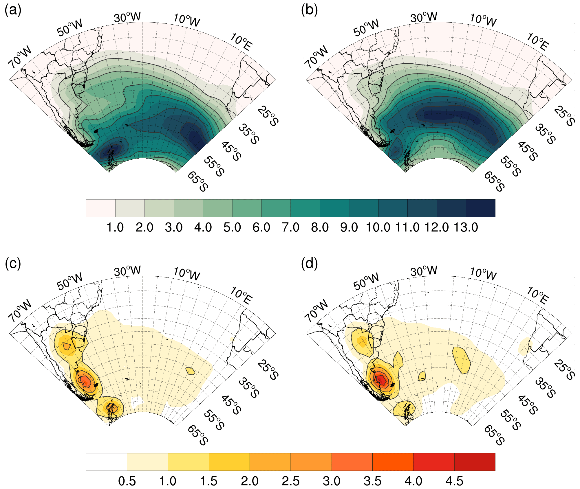
Figure B1 Cyclone (a, b) track and (c, d) genesis density in phase (a, c) A and (b, d) B of EOF1 of u₁₀. Dashed contours show 2 density unit intervals for the track and 1 for the genesis. Density unit is the system per year per area, where area is in 10⁶ km² (∼5^∘ spherical cap).

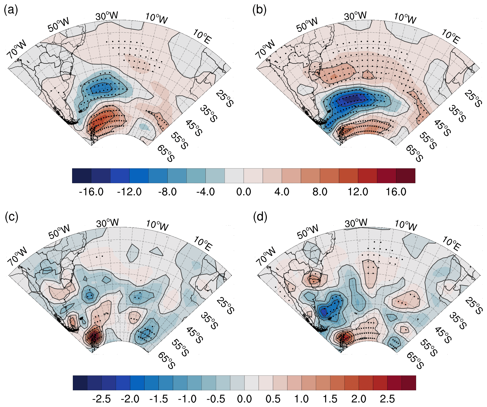
Figure B2 Cyclone (a, b) track and (c, d) genesis density differences between phases A and B of (a, c) EOF1 and (b, d) EOF2 of swh. Differences are calculated using phases A minus B and are also contoured by 5 density unit intervals for the track and 0.5 for the genesis. The black dots indicate where the difference is significant within a 95 % confidence level. Density unit is the system per year per area, where area is in 10⁶ km² (∼5^∘ spherical cap).

Appendix C

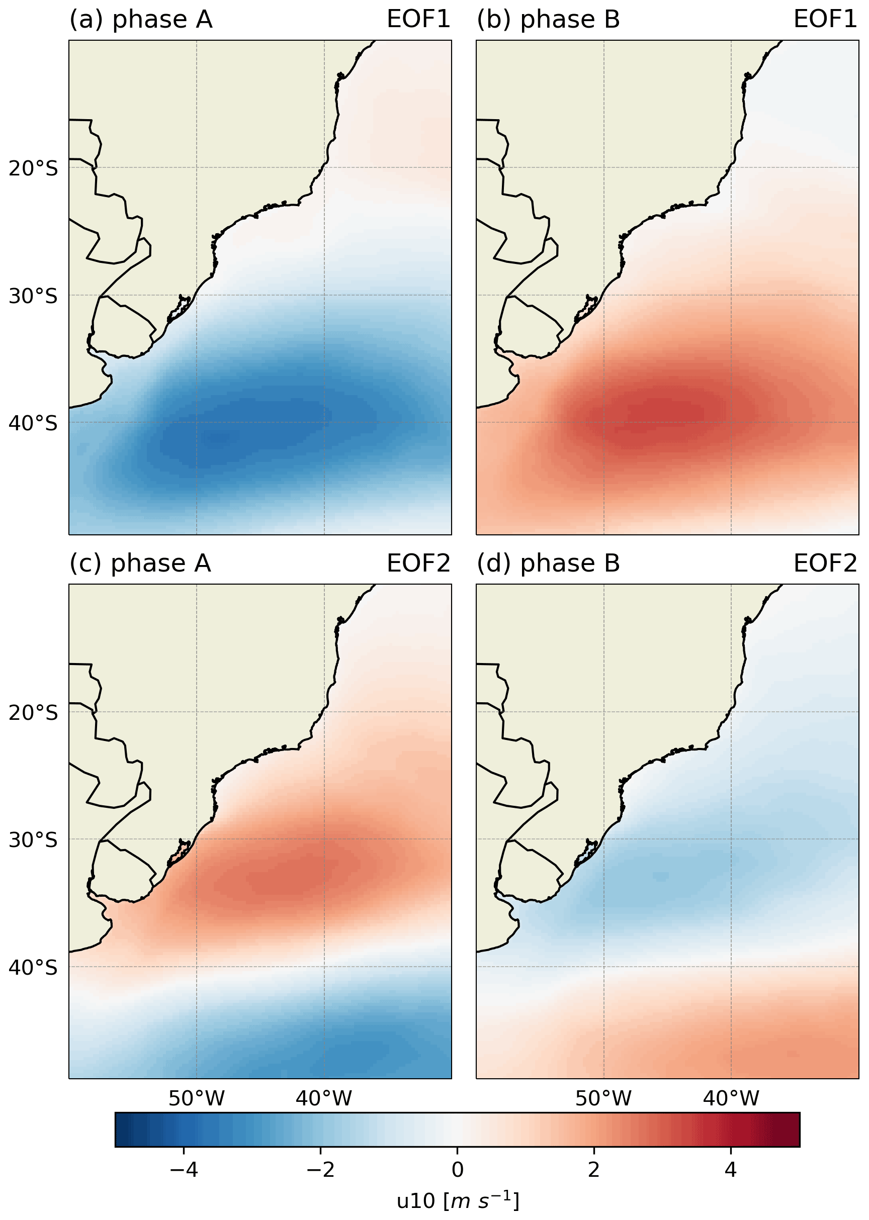
Figure C1 Composites of u₁₀ in phase A (a, c) and B (b, d) of the EOF1 (a, b) and EOF2 (c, d).

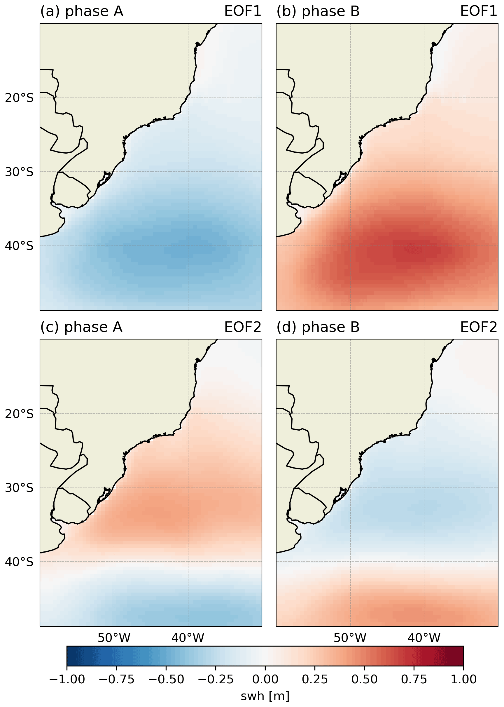
Figure C2 Composites of swh in phase A (a, c) and B (b, d) of the EOF1 (a, b) and EOF2 (c, d).