the Creative Commons Attribution 4.0 License.
the Creative Commons Attribution 4.0 License.
 | 07 Sep 2021
Emergence of representative signals for sudden stratospheric warmings beyond current predictable lead times
Bernat Jiménez-Esteve
Raphaël de Fondeville
Enikő Székely
Guillaume Obozinski
William T. Ball
Daniela I. V. Domeisen
Major sudden stratospheric warmings (SSWs) are extreme wintertime circulation events of the Arctic stratosphere that are accompanied by a breakdown of the polar vortex and are considered an important source of predictability of tropospheric weather on subseasonal to seasonal timescales over the Northern Hemisphere midlatitudes and high latitudes. However, SSWs themselves are difficult to predict, with a predictability limit of around 1 to 2 weeks. The predictability limit for determining the type of event, i.e., wave-1 or wave-2 events, is even shorter. Here we analyze the dynamics of the vortex breakdown and look for early signs of the vortex deceleration process at lead times beyond the current predictability limit of SSWs. To this end, we employ a mode decomposition analysis to study the potential vorticity (PV) equation on the 850 K isentropic surface by decomposing each term in the PV equation using the empirical orthogonal functions of the PV. The first principal component (PC) is an indicator of the strength of the polar vortex and starts to increase from around 25 d before the onset of SSWs, indicating a deceleration of the polar vortex. A budget analysis based on the mode decomposition is then used to characterize the contribution of the linear and nonlinear PV advection terms to the rate of change (tendency) of the first PC. The linear PV advection term is the main contributor to the PC tendency at 25 to 15 d before the onset of SSW events for both wave-1 and wave-2 events. The nonlinear PV advection term becomes important between 15 and 1 d before the onset of wave-2 events, while the linear PV advection term continues to be the main contributor for wave-1 events. By linking the PV advection to the PV flux, we find that the linear PV flux is important for both types of SSWs from 25 to 15 d prior to the events but with different wave-2 spatial patterns, while the nonlinear PV flux displays a wave-3 wave pattern, which finally leads to a split of the polar vortex. Early signs of SSW events arise before the 1- to 2-week prediction limit currently observed in state-of-the-art prediction systems, while signs for the type of event arise at least 1 week before the event onset.
- Article
(8705 KB) - Full-text XML
- BibTeX
- EndNote


Major sudden stratospheric warmings (SSWs) (Baldwin et al., 2021) are extreme wintertime circulation events of the Arctic stratosphere that are accompanied by a breakdown of the polar vortex which consists of strong circumpolar westerly winds in the polar stratosphere that form in fall and decay in spring. During a major SSW event the zonal-mean zonal wind in the stratosphere reverses in mid-winter from westerly to easterly, accompanied by an abrupt increase in temperatures in the entire polar stratosphere (Labitzke, 1981). SSWs are caused by the interaction between planetary waves and the mean flow in the stratosphere (Matsuno, 1971; McIntyre, 1982). The planetary waves are generated in the troposphere by flow over mountains, land–sea thermal contrast, and nonlinear synoptic scale wave–wave interactions (Charney and Eliassen, 1949; Scinocca and Haynes, 1998; Held et al., 2002; Domeisen and Plumb, 2012). The waves can propagate upward into the stratosphere if their wave number is sufficiently small (e.g., wave-1 and wave-2 components) and if the background zonal-mean zonal wind is eastward relative to the zonal phase speed of the waves (Charney and Drazin, 1961). When these planetary waves reach a critical level in the stratosphere, they break and deposit easterly momentum into the mean flow, resulting in a deceleration of the mean flow, which can eventually lead to a breakdown of the polar vortex, and an SSW event if the winds reverse to easterlies (Charlton and Polvani, 2007). The predictability limit for SSW events in state-of-the-art subseasonal prediction systems is around 1 to 2 weeks (Domeisen et al., 2020a). After an SSW event, the stratospheric anomalies can propagate downward to the lower stratosphere and influence the tropospheric weather for up to 2 months after the onset of events (Baldwin and Dunkerton, 2001; Kidston et al., 2015). For example, SSWs are found to be associated with an anomalously negative phase of the North Atlantic Oscillation (Domeisen, 2019) and an equatorward shift of the tropospheric extratropical jet streams (Baldwin and Dunkerton, 2001; Limpasuvan et al., 2004). The shift of the jet is crucial for the weather over North America and Europe, as it can lead to a larger probability of cold air outbreaks (Kolstad et al., 2010; King et al., 2019). Therefore, SSWs are thought to be an important source of predictability on subseasonal to seasonal (S2S) timescales over the Northern Hemisphere (NH) midlatitudes and high latitudes (Mukougawa et al., 2009; Scaife et al., 2016; Karpechko et al., 2017). Improving the predictability of SSW events may therefore help to enhance the forecast skill in the troposphere (Sigmond et al., 2013; Domeisen et al., 2020b).
Even though the polar vortex undergoes deceleration and disruption during all major SSW events, there are large differences amongst SSW events in terms of their dynamical evolution, vortex structure, and downward impact on the troposphere. Based on the geometry of the polar vortex at the onset of the event, SSWs can be classified into two types: (1) vortex displacement events, when the vortex is shifted off the pole, and (2) vortex split events, when the vortex is split into two parts (Charlton and Polvani, 2007). While displacement events are mainly attributed to the enhanced upward propagation of wavenumber 1 waves (hereafter: wave-1), split events are often related to strong wavenumber 2 waves (hereafter: wave-2) (Nakagawa and Yamazaki, 2006). In observations, major SSWs occur in about two out of three winters (Charlton and Polvani, 2007) with a similar frequency of split and displacement events (Butler et al., 2015), but with high decadal variability (Domeisen, 2019). However, if SSWs are classified based on the zonal wavenumber of the wave flux in the lower stratosphere, there are more wave-1 events than wave-2 events as not all split SSWs are dominated by wave-2 wave flux (Bancalá et al., 2012; Ayarzagüena et al., 2019). The occurrence of split events tends to be less predictable than that of displacement events, especially at lead times of 1–2 weeks (Taguchi, 2018; Domeisen et al., 2020a). Given the fact that the development of the two types of SSW events is considered to be different (Matthewman et al., 2009; Albers and Birner, 2014), the dynamical processes that lead to the breakdown of the polar vortex should be distinct between displacement (wave-1) and split (wave-2) events and should also be distinguishable from normal winter days (without SSWs). Therefore, understanding the dynamics of the vortex disruption and identifying signals that contribute to the vortex deceleration are crucial for improving the predictability of SSWs and of each type of event, and ultimately, of the weather at the Earth’s surface.
Since the stratospheric circulation is well described by Ertel's potential vorticity (PV) (McIntyre, 1982), the evolution of the polar vortex during SSWs can also be captured by the changes in the values and structure of the PV in the stratosphere. As discussed above, while the polar vortex undergoes breakdown in each major SSW event, the associated vortex structures are different for the two types of SSW events. Decomposing the PV into an empirical orthogonal function (EOF) basis, we can identify the PV structure that best describes the weakening of the polar vortex and subsequently investigate how its corresponding principal component (PC) changes with time. By projecting the other variables from the PV equation (i.e., the zonal and meridional wind) onto the EOF basis from PV, one can analyze the contribution of each term of the equation to the changes in the PC time series in order to identify the dynamical processes that are the most relevant for the weakening of the polar vortex. This approach was proposed by Aikawa et al. (2019) and called mode decomposition analysis. Aikawa et al. (2019) applied the mode decomposition analysis to diagnose the atmospheric blocking development in the eastern Pacific and central Atlantic and demonstrated that the blocking index can be faithfully reconstructed using only the first 10 EOF modes. The vorticity equation was then decomposed into three terms (i.e., linear advection, nonlinear mode-to-mode interaction, and dissipation), and their contribution to the combined time evolution of the first 10 PC time series was subsequently investigated. Their results showed that the nonlinear interaction terms contribute to the increase in the amplitude of the blocking index in both regions (eastern Pacific and central Atlantic) but that their contributions are different. Since each term in the vorticity equation can be linearly reconstructed using the EOF modes (that correspond to specific spatial patterns) and the PCs, this method allowed the identification of the wind and vorticity patterns that are crucial for the development of the blocking. As the results from Aikawa et al. (2019) indicate the effectiveness of mode decomposition analysis in studying dynamically driven events, we use the same method to study the development of SSWs, which are also driven by wave dynamics (e.g., Matsuno, 1971). Indeed, we find that the vortex weakening can be represented by the evolution of the EOF modes extracted from PV. We therefore employ a budget analysis of the PV equation in the stratosphere to quantify the contribution of each EOF mode to the dynamical processes that lead to the deceleration of the polar vortex and the subsequent onset of SSWs.
The onset of SSW events is associated not only with the anomalously large excitation of wave activity in the troposphere (Matsuno, 1971; Polvani and Waugh, 2004; Lindgren et al., 2018), but also with the stratospheric mean state and stratospheric wave anomalies prior to SSWs (Hitchcock and Haynes, 2016; Jucker, 2016; Birner and Albers, 2017; de la Cámara et al., 2019). Moreover, split and displacement SSW events exhibit distinct pre-warming evolutions (Charlton and Polvani, 2007; Matthewman et al., 2009; Bancalá et al., 2012; Albers and Birner, 2014). For example, the zonal wavenumber of the wave flux leading to the breakdown of the polar vortex can be different for the two types of SSW events (e.g., Bancalá et al., 2012). Some studies suggest that the explosive growth of wave amplitude is triggered by resonant behavior, which is also different between the two types of SSW events (e.g., Esler and Matthewman, 2011; Matthewman and Esler, 2011). Albers and Birner (2014) further suggest that different effects of planetary Rossby and/or gravity waves are responsible for producing the distinct vortex preconditioning that is conducive to developing the respective split and displacement SSW events. Given the distinct dynamical developments of the two types of SSWs, one should be able to observe different evolutions of the PV terms by the mode decomposition analysis for each type of SSW event. Since displacement (split) events are mainly related to wave-1 (wave-2) wave activity, in this study, SSWs are classified into wave-1 and wave-2 events based on the dominant wavenumber that leads to the breakdown of the vortex. As some studies point out that the dynamical process of the vortex breakdown starts earlier than the current predictable lead time (meaning the lead time on which an event can be predicted) of 2 weeks (Polvani and Waugh, 2004; Jucker and Reichler, 2018), one would expect to see signals indicative of the vortex breakdown appearing in the mode equation budget before the onset of the SSWs. Our goal in the current study is therefore to identify signals that are representative of SSWs, i.e., distinct from normal winter days, ahead of the vortex breakdown with lead times longer than 2 weeks and to distinguish onset signals for wave-1 and wave-2 events beyond the currently achieved predictable lead times.
The paper is organized as follows. Section 2 describes the data used in the analyses and the methodology behind the mode decomposition analysis. Section 3 shows the results of the analysis and their implications. Section 4 further provides the physical interpretation of the signals found in the mode equation budget by linking them with wave-mean flow interactions. Conclusions are given in Sect. 5.
2.1 Data and EOF basis
We use two datasets for analysis in this paper: (1) the ERA-Interim reanalysis (Dee et al., 2011) and (2) simulations from an intermediate complexity configuration of the Isca model (Vallis et al., 2018) (hereafter the Isca model). This version of the Isca model uses the model configuration from Jiménez-Esteve and Domeisen (2019), and it uses a T42 horizontal resolution and 50 vertical levels up to 0.02 hPa with 25 levels above 200 hPa. The model includes moist and radiative processes through evaporation from the surface and fast condensation. Water vapor in the atmosphere interacts with a multiband radiation scheme (Mlawer et al., 1997) and a simple Betts–Miller convection scheme (Betts and Miller, 1986). The CO2 concentration is fixed at 300 ppm, and the seasonal cycle of ozone in the stratosphere is prescribed based on the ERA-Interim (1979–2016) climatology. For the lower boundary conditions, the Isca model uses realistic topography and the continental outline from the ECMWF model, and sea surface temperatures (SSTs) are prescribed. The model does not include a representation of clouds, interactive chemistry, or gravity wave drag. In this paper, we use the experiment that uses prescribed strong El Niño-like SST anomalies as described in Jiménez-Esteve and Domeisen (2019). The motivation to use this model experiment is that it produces a realistic climatology and a frequency of SSWs that is similar to the reanalysis.
For ERA-Interim, we use daily mean fields of potential vorticity (PV) P, zonal wind u, and meridional wind v at the 850 K isentropic level from 1979–2018 with a horizontal resolution of . Only data north of 30∘ N (24 latitude values by 144 longitude values leading to a total of D=3456 grid points) from the winter season (October to April, 8490 d in total) are included in the analysis. For the Isca model simulations, the daily vertical gradient of potential temperature (θ), zonal wind u, and meridional wind v are interpolated to the 850 K isentropic surface from pressure levels. The Isca model data contain a total of 130 years, corresponding to 27 300 winter days. The PV is computed as
where P is Rossby–Ertel's PV (Hoskins et al., 1985), ζθ is the relative vorticity on the isentropic surface, θ is the potential temperature, f is the Coriolis force, g is the gravity, and p is the pressure. Note that in this work potential vorticity (PV) refers to Rossby–Ertel's PV.

Figure 1The first 10 EOF spatial patterns of PV at 850 K (E1, E2, …, E10) of the combined set of basis vectors as described in the text using ERA-Interim daily data. The percentage number indicates the variance explained by each EOF.
The PV data (for both the ERA-Interim reanalysis and the Isca model) are further decomposed into (1) the daily climatology, obtained by computing the daily mean values of PV over all available years, and (2) daily anomalies with respect to the climatological seasonal cycle. Given the limited number of years in the reanalysis, we also applied a 30 d running mean to the daily climatology to remove the high-frequency variability and repeat the analysis performed in the study. The results are almost identical to the ones using climatologies without low-pass filtering, which is mainly due to the fact that applying principal component analysis (PCA) acts as a filter and indicates the importance of the low-frequency components in the evolution of the polar vortex. In the following figures, we show the results using climatologies without low-pass filtering. The EOF modes of the PV and their corresponding PC time series (later used in the mode decomposition analysis) are obtained by employing PCA on the daily PV anomalies at 850 K. The procedure consists of applying PCA twice, as described in the following. We apply a first PCA only to the PV data around the onset date of all SSWs (from −10 to +5 d around the onset date). The motivation behind this first PCA is to obtain a mode that captures the characteristics of SSWs. The spatial pattern of the resulting first EOF mode (E1∈ℝD) is shown in the first panel in Fig. 1, with a wavenumber 0 structure centered at the pole. Next, we project all the winter data (October to April) onto the subspace orthogonal to E1 by subtracting from the winter data their projection onto E1, and then we perform a second PCA on this projection. The resulting data do not contain any information from E1 since it is in the space orthogonal to E1 and yield a total of D=3456 modes {E2, …, ED+1} (equivalent to the number of grid points). Combining the first EOF mode E1 from the first PCA with the D EOF modes from the second PCA forms an orthogonal basis for all the winter data, referred to in the following as the “combined set of basis vectors”. Figure 1 shows the spatial pattern of the first 10 EOF modes that explain together ≈71 % of the variance of the PV anomalies of all winter days in the ERA-Interim data. The spatial patterns of the first 10 EOF modes of the PV anomalies in the Isca model data are shown in Fig. C1. We note that the EOF modes cannot be interpreted by default as physical modes as also discussed in Dommenget and Latif (2002) and Monahan et al. (2009). Here, since E1 is derived using only days around SSWs (−10 to +5 d around the onset date of SSWs) and displays a clear zonally symmetric structure, the physical process represented by the variation in E1 can be interpreted as representing the changes in the strength of the polar vortex during SSWs. In ERA-Interim, the variance explained by E1 (15.8 %) for all the winter data is slightly smaller than that of E2 (16.8 %), as shown in Fig. 1. The EOF modes are orthogonal and therefore satisfy the following relationship of the inner product :
where δmn is the Kronecker delta function, and Ω is the region poleward of 30∘ N. As mentioned above, the main motivation for applying the double PCA approach to obtain the EOF basis rather than directly applying PCA once to all the winter days is that E1 is computed from the days around the onset day of SSWs, and its variability is therefore closely linked to SSW events, as can be seen from Fig. 2. The PC time series of all winter days associated with E1 (Fig. 2) is highly correlated with the polar-cap-averaged temperature at 30 hPa, thus being a good representation of SSWs (Blume et al., 2012). The evolution of the first PC (for all winter data) therefore enables us to better understand the vortex breakdown process.
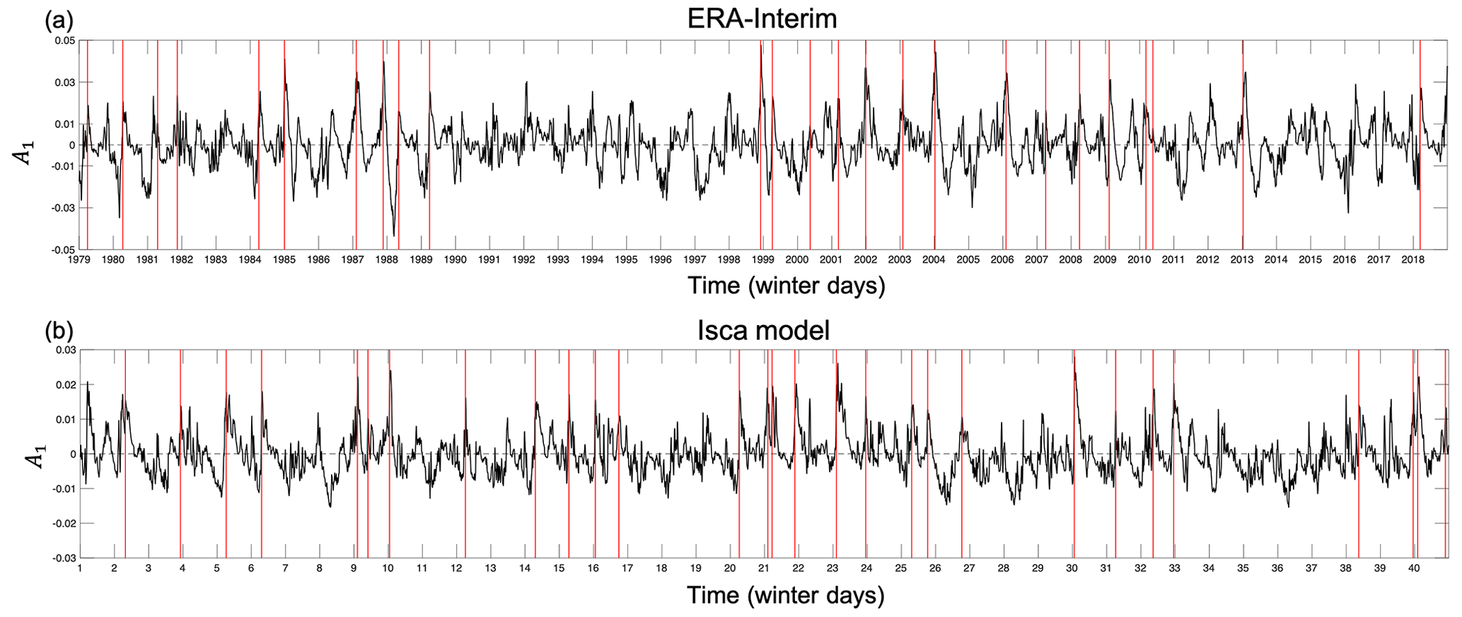
Figure 2The PC time series (A1) of all winter days corresponding to the first EOF mode E1 using (a) ERA-Interim reanalysis data and (b) Isca model output data. (a) All winter days (from October to April) are shown and in (b) only the winter days for the first 40 years are shown as an example. The PC time series for winter days of the remaining 90 years in the Isca model can be seen in Fig. C2. The red vertical lines indicate the onset dates of SSW events.
2.2 Mode decomposition analysis
Following the methodology from Aikawa et al. (2019), the mode decomposition analysis is applied to the PV conservation equation to study the dynamical development of SSW events. The anomalous PV equation on an isentropic surface can be written by separating the daily anomalies from the daily climatological mean for 1979–2018 as
where P is the PV, V is the wind vector field, and F is the forcing term (computed here as residual). The subscript “c” refers to daily climatology, and “a” refers to daily anomalies. The anomalous PV tendency equals the sum of linear effects that consist of the advection of daily anomalous PV by climatological wind vector (Vc⋅∇Pa) and the advection of climatological PV by the anomalous wind vector (Va⋅∇Pc) and the nonlinear effects of the advection of anomalous PV by the anomalous wind vector (Va⋅∇Pa).
For the mode decomposition analysis of the PV equation, we focus only on the time frame between 50 and 1 d prior to the onset day of SSW events as the goal of this study is to identify signals that precede SSWs. We project the PV field (obtained by concatenating the data from −50 to −1 d before the onset of all SSWs) onto the first d=1000 modes of the combined set of basis vectors {E1, E2, …, Ed} and get the corresponding PC time series, denoted as {A1, A2, …, Ad}. We found that the first d=1000 modes (which in total explain 99.9 % of the variance of PV as shown in Fig. A1a) are sufficient to reproduce the actual rate of change of the PCs. The PV daily anomalies (Pa) can be expressed as the linear combination of {E1, E2, …, Ed} with coefficients {A1, A2, …, Ad}. For the wind vector daily anomalies (Va), the temporal evolution of PV is correlated with that of the wind fields. Therefore, it is possible to obtain a set of spatial patterns {U1, U2, …, Ud} for Va by regressing Va onto the PC time series of PV, {A1, A2, …, Ad}. Note that the spatial patterns {U1, U2, …, Ud} are not orthogonal as they are not obtained through an EOF mode decomposition. The Va can then be represented as the linear combination of with coefficients A1, A2, …, Ad. Then, by substituting the projection of Pa and Va onto the PC time series into Eq. (3) and taking the inner product between Eq. (3) and a given EOF mode Ek, we obtain the mode equation budget of the rate of change (or tendency) of Ak as (detailed derivation in Appendix A)
where is the eigenvalue associated with mode Ek, , Vc⋅∇En〉 and , Un⋅∇Pc〉 are the inner products between the linear advection terms (Vc⋅∇En and Un⋅∇Pc) and Ek, Nkmn=〈Ek, Um⋅∇En〉 is the inner product between the nonlinear advection term (Um⋅∇En) and Ek, and is the residual term. The sum of the two linear advection terms gives the total linear advection term. Using Eq. (4), we then compute the contribution of each mode to the linear and nonlinear advection terms and thus to the total rate of change of Ak to determine which modes (or combinations of modes) play an important role in identifying signals distinguishing SSWs from normal winter days.
From the power spectrum of each PC time series Ak (see Fig. A1b), the power of A1 to A25 is concentrated at frequencies lower than once a week, which is different from the power spectrum of the other PCs beyond A25. Based on these power spectra, here we consider the associated modes E1 to E25 as low modes, which together explain around 85 % of the total variance, and modes beyond E25 as high modes. To separate the contributions from low and high EOF modes, the summation over all modes from Eq. (4) is divided into the summation of low modes and that of high modes. Thus, Eq. (4) can be written as
where l=25 represents the nth mode that is treated as the last low mode; Llow and Lhigh are the linear low and high mode terms, respectively; Nlow–low, Nlow–high, and Nhigh–high are the contributions from nonlinear low–low, low–high, and high–high mode interactions, respectively; Ltotal is the total linear PV advection as , and Ntotal is the total nonlinear PV advection as . We performed sensitivity tests for a range of l values, and our results and conclusions are robust for values of l>25. Moreover, the contribution from modes higher than l=25 is very small (not shown). In this study, we only focus on the rate of change of the first PC time series due to the strong relationship between A1 and SSWs.
2.3 SSW definition
The major SSW definition follows the criterion of Charlton and Polvani (2007), based on the reversal of the daily zonal-mean zonal winds at 10 hPa and 60∘ N and a return to westerlies afterward for at least 10 consecutive days before the final warming. Two events in the same season are treated as distinct SSWs if they are separated by at least 20 d. The central dates of split and displacement SSW events in ERA-Interim before 2014 are taken from Karpechko et al. (2017) and consist of 11 split events and 12 displacement events. In addition, we added the SSW event in 2018, which is classified as a split event based on the vortex geometry (Charlton and Polvani, 2007). The definition of wave-1 and wave-2 SSW events is based on the eddy heat flux at 100 hPa and 60∘ N similar to Bancalá et al. (2012). If the wave-2 component of eddy heat flux is larger than the wave-1 component by 15 Km s−1 in the period of −2 to 0 d before the SSW event for at least 1 d, then the SSW event is classified as a wave-2 event, otherwise as a wave-1 event. Note that the time window around the SSW event (day −2 to day 0) that is used to classify the type of event is shorter than that in Bancalá et al. (2012). The reason for using a shorter window is to reduce the overlap between the time interval used to define the type of SSW event and the lead times that emerge as relevant in the predictability of wave-1 vs. wave-2 events. According to this definition, there are 18 wave-1 and 7 wave-2 SSW events in ERA-Interim. Note that not all split events are dominated by wave-2 wave flux (only 6 out of 12 split SSWs are also classified as wave-2 events), while one displacement event is dominated by wave-2 wave flux according to this definition.
2.4 Interpretation of results from mode decomposition based on PV flux
Up to this point, our mode decomposition analysis does not employ any explicit approximation. In this section, we will demonstrate how Ltotal and Ntotal are related to the poleward PV flux, which can help to illustrate the physical interpretation of the results obtained from the mode decomposition analysis.
In order to provide a physical interpretation for each term in Eq. (5) and understand the physical process that can lead to the disruption of the polar vortex, we introduce the poleward flux of PV on an isentropic surface given by Tung (1986) as
where ℱ is the Eliassen–Palm flux (EP flux); P is the potential vorticity; v is the meridional wind; ρθ is the density in isentropic coordinates, defined as ; and ϕ is the latitude. The brackets denote the zonal mean, one asterisk denotes the deviation from the zonal mean, and two asterisks denote the deviation from the density-weighted zonal average, as in
The formulation of the PV flux in Eq. (6) is also equivalent to that defined using , as in Eq. (4.5) in Tung (1986). The left-hand term in Eq. (6) is the EP flux pseudo-divergence, and the right-hand term in Eq. (6) is the zonal-mean northward flux of PV on the isentropic surface. According to Tung (1986), the PV flux corresponds to the pseudo-divergence of the EP flux along isentropic surfaces and acts as the net eddy forcing term of the mean flow. Note that the pseudo-divergence of the EP flux is used here (instead of the divergence) due to the fact that the density on isentropic surfaces changes with time, which is the main difference from the conventional EP flux (Edmon et al., 1981).
Using the concepts of PV flux and EP flux pseudo-divergence, we rewrite Eq. (3) as
The second to fourth terms on the left-hand side are the linear and nonlinear terms of the density-weighted PV flux divergence, while the last term is the local density tendency. Since the density-weighted PV is proportional to vorticity, the second to fourth terms can be interpreted as the dynamical contribution to the PV evolution. On the other hand, since the density tendency is inversely proportional to the temperature tendency, the fifth term can be interpreted as the thermodynamic component of the PV evolution. Equation (8) is derived by converting the advection terms in Eq. (3) into density-weighted flux divergence using the continuity equation. Taking the inner product between Eq. (8) and E1 and neglecting the longitudinal variation in E1 given its wavenumber-0 structure, i.e., E1≈E1(ϕ), we obtain an approximation of the linear and nonlinear terms in Eq. (8) (a detailed derivation is provided in Appendix B):
where v is the meridional wind, a is the radius of the Earth, and ϕ is the latitude with ϕ1=30∘ N and ϕ2=90∘ N. Next, we combine the mode equation budget from Eq. (5) with the zonal-mean PV flux from Eq. (6). Based on the relation shown in Eq. (6) and the fact that from the zonal momentum equation, one can further obtain the following relation:
Equation (10) shows that the meridional gradient of zonal-mean PV flux is connected to the vorticity tendency , which is the dynamical component of the rate of change of A1.
As shown in Fig. 1, the first EOF spatial pattern E1 of the PV daily anomalies in ERA-Interim takes the shape of a wavenumber-0 structure with a negative anomaly at the pole. Thus, a positive1 (negative) value of A1 (PC time series of E1) indicates a weakening (strengthening) of the polar vortex. For example, Fig. 2a shows the corresponding A1 for all winter days of ERA-Interim (8490 d in total), and the red vertical lines indicate the onset day of the SSW events. Before SSW events occur, A1 increases significantly and is strongly positive on the onset day, indicating a weakening and breakdown of the polar vortex. Similar EOF spatial patterns are found for the Isca model data (Fig. C1), together with a similar increase in A1 when approaching the SSW central day (Fig. 2b). The Isca model data consist of a total of 130 years of simulation, corresponding to 27 300 winter days, of which Fig. 2b only shows the winter days from the first 40 years as an example. By understanding what contributes to the changes in A1, we extract information that helps explain the breakdown of the polar vortex during SSW development. We compute the mode equation budget of A1 using daily data concatenated for the period −50 to −1 d prior to the onset day for all SSW events. There are a total of 25 SSWs in the ERA-Interim reanalysis data and 78 SSWs in the 130-year simulation in the Isca model. Next, we show the composite of SSW events for both reanalysis and the Isca model data.
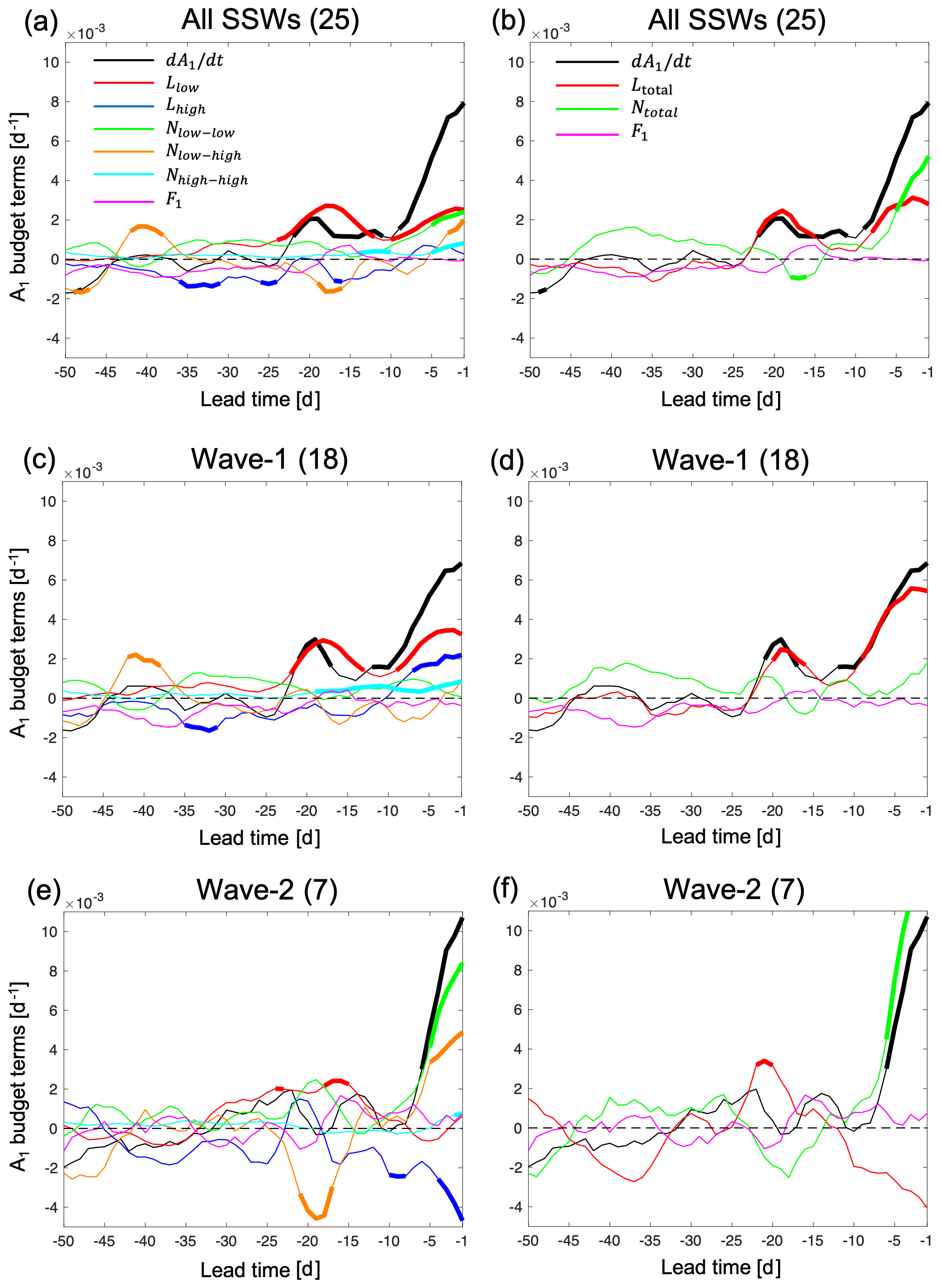
Figure 3The SSW composite of the A1 budget as a function of lead time from 50 to 1 d before the onset of events in ERA-Interim. (a, b) Composite of all 25 SSW events; (c, d) composite of the 18 wave-1 events; (e, f) composite of the 7 wave-2 events. Panels (a, c, e) show each term of the mode equation budget (Eq. 5) separately, and (b, d, f) show the total linear term and the total nonlinear term for the different subsets of SSWs. The number in the bracket in each panel title indicates the number of SSW events. A 5 d running mean is applied to all lines. Bold lines indicate values that are outside the percentile range 2.5 to 97.5 of normal winter day values from bootstrapping as described in the text. The representation of each line color in (c, e) and (d, f) is the same as the legend in (a) and (b), respectively.
3.1 Mode equation budget for ERA-Interim
Figure 3 shows the SSW composite of the A1 mode decomposition budget. The first, second, and third rows show the results of the composites of all SSW events, wave-1 SSW events, and wave-2 SSW events, respectively. We apply a 5 d running mean to all lines in Figs. 3–6 to remove the high-frequency fluctuations. The bold lines in Figs. 3–6 indicate the values that are outside the percentile range 2.5 to 97.5 of normal winter day values, which is computed via a bootstrapping procedure described as follows. In each bootstrap sample, we randomly select with replacement 25 sets of 50 consecutive non-SSW winter days (excluding the 50 d before each SSW) across the different years. We then calculate the mean of these 25 sets of non-SSW days to represent the “composite” of normal winter days. We repeat the bootstrap resampling procedure B=1000 times and compare the SSW composite against the percentiles 2.5 and 97.5 of the B bootstrap samples. The same procedure is also applied for the two types of SSWs and for the Isca model data, using the number of SSWs in each dataset as the number of sets of consecutive non-SSW winter days in the bootstrapping. If we only select 50 consecutive non-SSW winter days in December, January, February, and March (months when SSWs occur) to reflect the temporal distribution of SSWs, we obtain qualitatively similar results as when using non-SSW days for all winter months. Here we present the results with the bootstrapping using non-SSW days for all winter months. The reconstructed A1 tendency (black line in Fig. 3) is computed from Eq. (5). The left panels show each term in Eq. (5), while the right panels show the combined effect of all linear (red) and all nonlinear (green) terms without separating the contributions from low and high EOF modes. Figure 3a indicates that around 25 d before the central day of SSWs starts to increase, and the increase shows a steeper slope around 10 d before the SSW event, leading to a large positive A1 on the central day as shown in Fig. 2a. Along with the increase in , Llow (red) also increases and is well correlated with the A1 tendency (r=0.8). In fact, Llow starts to increase from 35 d before the events, but its effect is offset by other terms and it becomes the only contributor to the increase in at 25 to 15 d leads. The nonlinear term Nlow–low (green) shows a rapid increase around 2 weeks before the SSW event and, together with the linear term Llow, significantly contributes to the changes in A1. The high-frequency components are overall weaker than the low-frequency terms, especially the Nhigh–high (cyan), but the Nlow–high (orange) has large variations and tends to offset the effect of Llow–low at −25 to −15 d before the vortex weakening.
The contributions from each term are different between the composites of wave-1 vs. wave-2 events (Fig. 3c and e). The amplitude of Lhigh (blue) is large at around 1 week before the event, and the nonlinear terms are overall small for wave-1 events (Fig. 3c) when compared to wave-2 events (Fig. 3e). The amplitude of Nlow–low is the largest starting 1 week before the onset for the wave-2 events. To better illustrate the different contributions of linear and nonlinear advection terms in Eq. (5) to the increase in in the two types of SSW events, we combine all the linear terms (Ltotal) and all the nonlinear terms (Ntotal) and show the results in the right panels of Fig. 3. The linear advection term has the most important contribution from around 25 to 15 d before both SSW event types, and the nonlinear advection term becomes more dominant from day −15 to the onset of the wave-2 SSW events (Fig. 3f). On the other hand, the linear advection term plays a central role from day −25 to day 0 for the wave-1 SSWs (Fig. 3d). The distinct contributions from the linear and nonlinear advection terms for wave-1 vs. wave-2 events indicate that the processes leading to the vortex breakdown of the two types of SSW events are dynamically different. The simultaneous contributions from linear and nonlinear terms in the all-SSW composite (Fig. 3a and b) can be viewed as being due to the average over wave-1 and wave-2 SSW events within the composite (Fig. 3b). For both types of events, the process captured by the increase in the linear advection term initiates the weakening of the polar vortex around 1 month before the event and plays a central role until day −10. Around 10 d before the event, the linear (nonlinear) advection term has the dominant contribution for the breakdown of the vortex for the wave-1 (wave-2) events, while the nonlinear (linear) terms are less important or even counteract the increase in . Therefore, the relative importance of the linear and nonlinear terms emerges as a good indicator of the type of SSW events with a lead time of around 10 d prior to the events.
The relative importance of the linear and nonlinear advection terms for the two types of SSW events is similar to that of the stratospheric wave amplitude of the wavenumber 1 and 2 components for wave-1 and wave-2 SSW events as shown in Bancalá et al. (2012). From their composite analysis of the wave-2 SSW events, the wave-2 component of the geopotential height anomaly in the stratosphere is significantly positive from day −10 to day 0, and the anomalous increase in the wave-1 component was found in the period from day −30 to day −10. In Fig. 3 we find that the linear and nonlinear advection terms behave similar to the wave-1 and wave-2 components of the upward-propagating wave activity. Consistent with the two periods in Bancalá et al. (2012), the evolution of linear and nonlinear terms can be separated into two different time periods, with one from day −25 to day −15 and the other from day −10 to day 0. Since the displacement (split) SSW events are mainly attributed to the enhanced upward propagation of wave-1 (wave-2) (Nakagawa and Yamazaki, 2006; Bancalá et al., 2012), we also look into the contributions of linear and nonlinear terms to for displacement and split SSW events (shown in Fig. D1), with very similar results. Comparing Fig. D1a, b with Fig. 3c, d, the behaviors of each term, the total linear term, and the total nonlinear advection term are very similar as most of the displacement events are wave-1 events (only the event in March 2000 is a wave-2 event). Among the 12 split SSWs, six events are dominated by wave-1 wave flux, and most of them do not have a clear split-type behavior as those dominated by wave-2 wave flux. On the other hand, comparing Fig. D1c, d to Fig. 3e, f, the differences between linear and nonlinear terms are more obvious for wave-2 SSWs as only half of the split events are included in wave-2 events. The behavior of the linear and nonlinear PV advection terms for wave-1 and wave-2 SSWs as shown in Fig. 3d and f (for displacement and split SSWs, see Fig. D1) is comparable to the results in Smith and Kushner (2012), who showed that displacement (split) SSW events are preceded by pronounced linear (nonlinear) vertical wave activity. Our results suggest that the linear and nonlinear contributions are more strongly related to the dominant wavenumber wave forcing than to the vortex geometry.
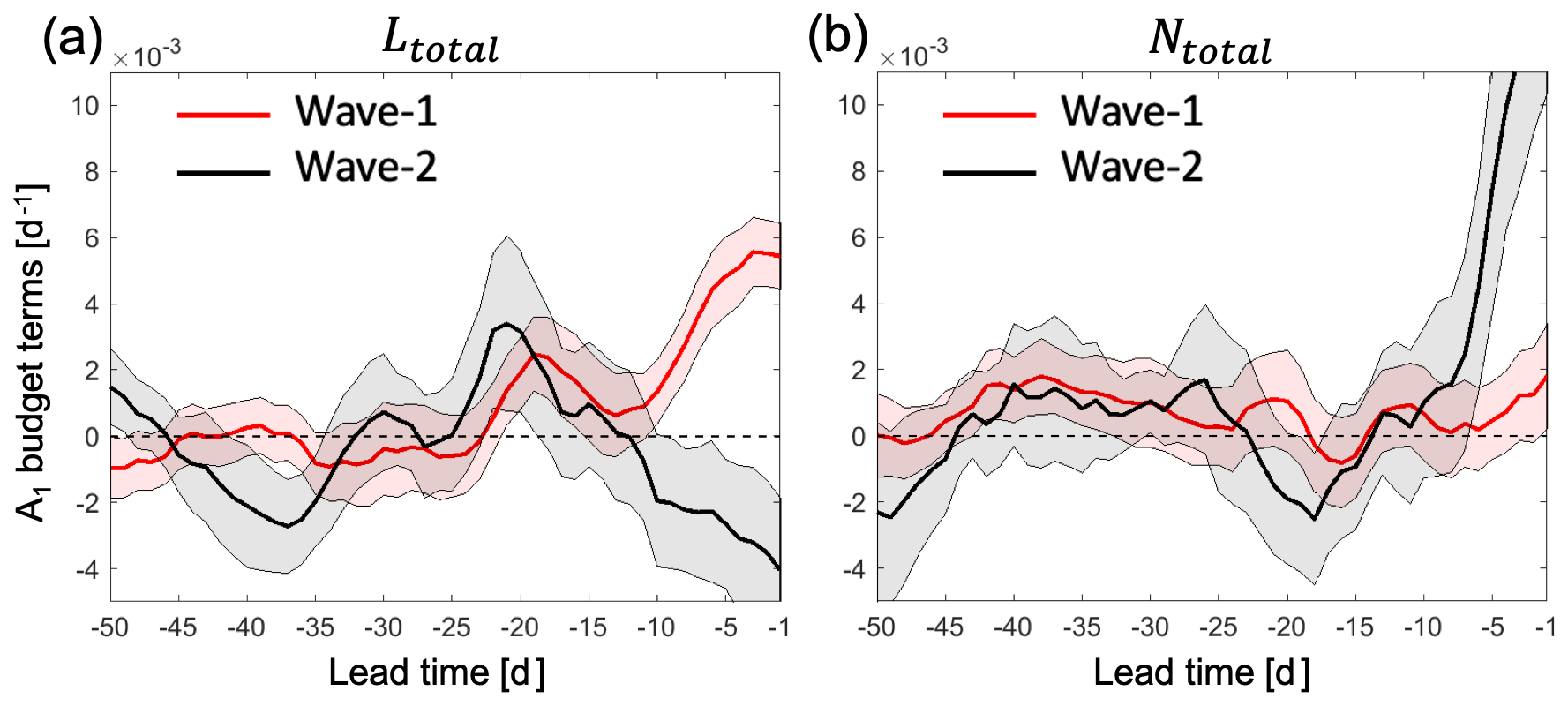
Figure 4The comparison of the A1 budget of the bootstrapping between wave-1 and wave-2 SSW events as a function of lead time from 50 to 1 d before the onset of events in ERA-Interim. (a) Sum of linear advection terms, and (b) sum of nonlinear advection terms for wave-1 events (red) and wave-2 events (black). A 5 d running mean is applied to all lines. Bold lines and the shading indicate the mean and ±1 SD (standard deviation) of a bootstrapping using B=1000 samples.
In order to examine the significance in the differences and the robustness of the relative importance of the linear and nonlinear advection terms for the two types of SSW events, we perform bootstrapping on individual wave-1 and wave-2 events with replacement, respectively. We repeat the resampling B=1000 times and compute the means and the standard deviation for the sum of linear and nonlinear terms. The results of the bootstrapping are shown in Fig. 4. There is almost no overlap between the ± 1 SD (standard deviation) of wave-1 (red) and wave-2 (black) events in either the total linear advection (Fig. 4a) or the total nonlinear advection (Fig. 4b) term at 1 week before the onset of the events. In particular, the separation of the wave-1 and wave-2 events in the total linear advection term is as early as 10 d before the onset of the events. Figure 4 demonstrates the significance and robustness of the differences in the contribution of the linear and nonlinear advection terms to in the wave-1 and wave-2 SSW events, respectively, at least up to 1 week before the events. Another point to highlight is that significant anomalies of the linear terms are observed around 20 d before both types of SSW events, which is beyond the current predictability limit of SSWs of 1–2 weeks.
3.2 Mode equation budget for the Isca model
Given the limited number of SSW events in the reanalysis data and to further examine the characteristics and robustness of the linear and nonlinear term contributions to the vortex breakdown, we now apply the same analysis as for ERA-Interim to the output of the Isca model experiment. We use the methodology from Sect. 2 to extract the EOF modes (spatial patterns) and apply the mode decomposition analysis to the data concatenating 50 to 1 d prior to the 78 SSWs present in the model data. The EOF spatial patterns derived from the model output are similar to those derived from ERA-Interim, especially the first 10 EOF modes (Fig. C1), indicating that the model is able to capture the PV features as in the reanalysis.
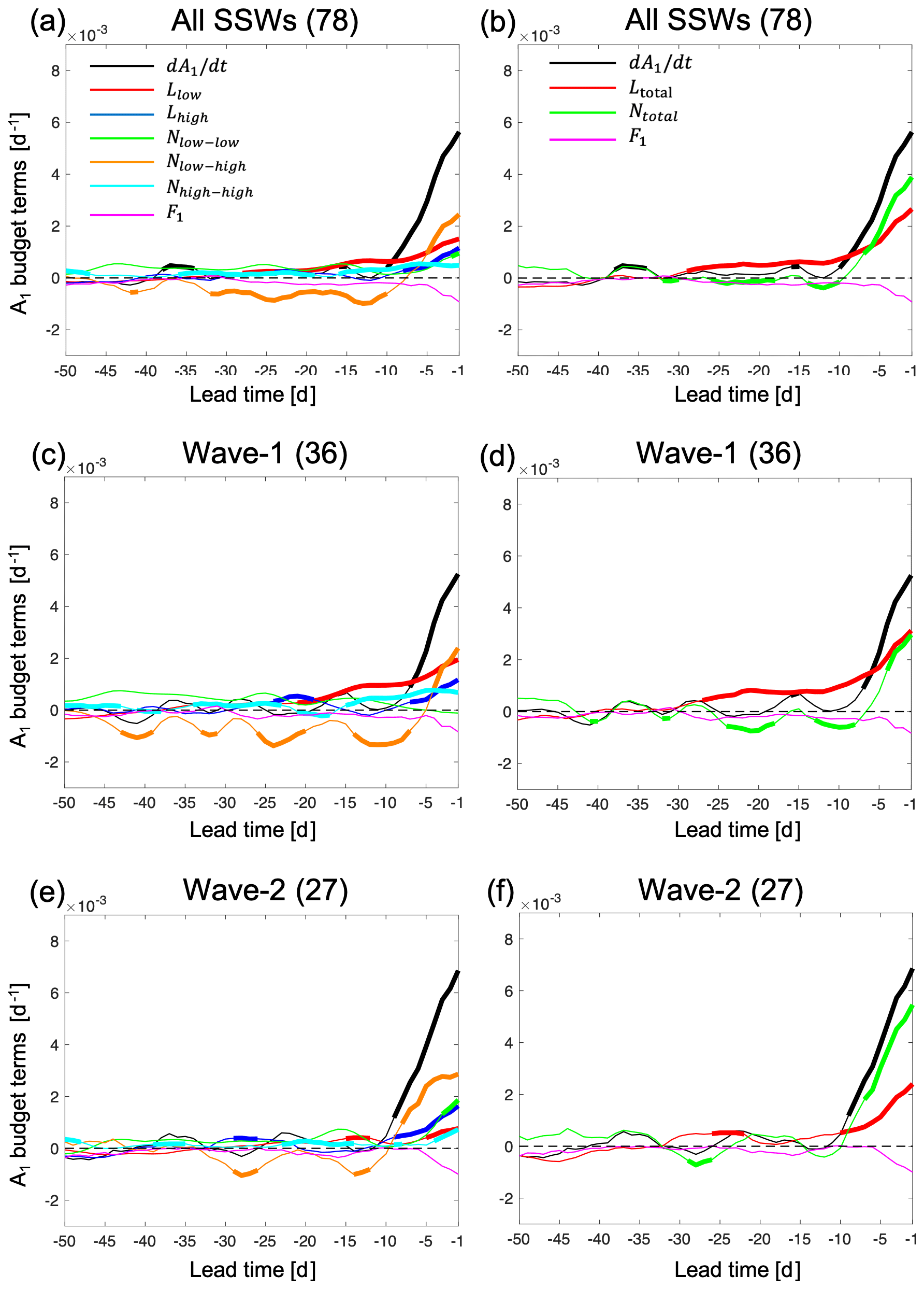
Figure 5The composite of A1 budget as a function of lead time from 50 to 1 d before the onset of the events in the Isca model output. (a, b) Composite of the total 78 SSW events, (c, d) composite of the 37 wave-1 events, and (e, f) composite of the 26 wave-2 events. (a, c, e) show each term of Eq. (5) separately, and (b, d, f) show the total linear term and the total nonlinear term for the different subsets of SSWs. All lines are smoothed by a 5 d running mean. Bold lines indicate the values that are outside the percentile range 2.5 to 97.5 of normal winter day values from bootstrapping as described in the text. The representation of each line color in (c, e) and (d, f) is the same as the legend in (a) and (b), respectively.
Figure 5 shows the results of the A1 budget for the SSW composites. Similar to the results in ERA-Interim (Fig. 3), the linear term Llow starts to increase at around day −25, but the increase in starts at around day −10 (Fig. 5a), which is later than that in ERA-Interim (around day −25). In the period of day −10 to day 0 of SSWs, Nlow–high increases rapidly. The increasing Nlow–high and Llow lead to a rapid increase in . We note that in the 2 d before the onset date, the magnitude of the wave-1 and wave-2 wave fluxes is similar (with differences < 5 Km s−1) in some SSW events simulated in the Isca model. In order to make a clearer separation between wave-1 and wave-2 SSWs, we exclude events with the difference in the magnitude of wave-1 and wave-2 heat flux at 100 hPa and 60∘ N smaller than 5 Km s−1 as these events cannot be clearly categorized as either wave-1 or wave-2 events. Therefore, in the model we have 36 wave-1, 27 wave-2, and 15 unclassified events. Figure 5c shows that Llow for SSWs increases and starts to differentiate from normal winter days starting at a lead of 20 d for wave-1 SSWs. Different from the A1 budget of wave-1 SSWs in ERA-Interim (Fig. 3c), Nlow–high starts to increase from day −7 and becomes an important contributor to . For wave-2 SSWs, Fig. 5e shows that Nlow–high is the main contributor to the increase in from day −10, and Nlow–low and Lhigh are the second largest contributors to from day −5, which is different from the evolution of Lhigh for wave-2 SSWs in ERA-Interim (Fig. 3e). In both types of events, Llow starts to increase at around day −20, which helps to weaken the polar vortex in the preconditioning stage and is similar to the evolution of Llow (with a smaller amplitude) in the same period in ERA-Interim. The effects of Ltotal and Ntotal are shown in the right panels in Fig. 5. The evolution of Ltotal and Ntotal, and thus of , for the Isca model (Fig. 5b) is similar to the evolution of these terms for the ERA-Interim data (Fig. 3b), indicating that the Isca model successfully reproduces the vortex breakdown in the 10 d preceding the SSWs. The increase in can therefore be used to predict the occurrence of SSWs with 1–2 weeks lead time. Even though the distinct increase in only shows up at around day −10, Ltotal actually increases as early as day −29. However, this amplification in the linear term is offset by the nonlinear and forcing terms, which leads to a near-zero . Figure 5d and f show the evolution of Ltotal and Ntotal of the wave-1 and wave-2 SSW composites, respectively. Different from wave-1 events in ERA-Interim, the linear and nonlinear terms are equally important. However, when comparing wave-1 with wave-2 composites, one can still see the difference in the relative importance of the linear and nonlinear terms for the two types of SSWs. The nonlinear term is stronger in wave-2 SSWs than in wave-1 SSWs and is more than twice as large as the linear term 1 week before the central day (Fig. 5f). Thus, our finding from ERA-Interim that the linear (nonlinear) term is important for wave-1 (wave-2) events is also true for the Isca model data. The main differences compared with the reanalysis data are that exhibits a substantial increase only from day −10, and the variations in all terms in Eq. (5) are overall small before day −10, which could potentially limit the predictability of SSWs in the Isca model. Different reasons might be able to explain the differences in results between the Isca model and the reanalysis, e.g., different model complexities (e.g., lack of parameterizations for gravity waves breaking and interactive ozone chemistry in the Isca model) or the coarse model horizontal resolution (T42), both of which might lead to an underestimation of some of the high-frequency variability in comparison with the reanalysis. Another important difference is that in the Isca model the nonlinear term displays larger values for both types of SSWs compared to the reanalysis. This latter behavior might be related to the stronger SSW sensitivity to wave-2 forcing in the idealized models (e.g., Isca model) where most of the SSWs are likely triggered by wave-2 activity (Gerber and Polvani, 2009), in contrast with wave-1 which seems to be more dominant in more complex general circulation models or reanalysis datasets (see for example Fig. 3 in Ayarzagüena et al., 2018). Note that even when classifying an SSW event as a wave-1 event in the model, its wave-2 component, although weaker than the wave-1 component, might still play an important role in the overall evolution of the event.
In our analyses above, we found that the persistent positive values of and its contributors that emerge during the vortex breakdown, such as during SSWs, are significantly different from the values observed during normal winter days. Additionally, the signals identified as representative of wave-1 and wave-2 events are also different. We also observed that the signals that are characteristic of SSWs emerge as early as 20–25 d before the onset of SSWs. Given that these results hint that SSWs are potentially predictable at longer lead times, i.e., beyond the current predictability limit of 1–2 weeks, in this section we provide a physical interpretation of these signals that we identified through the mode decomposition analysis.
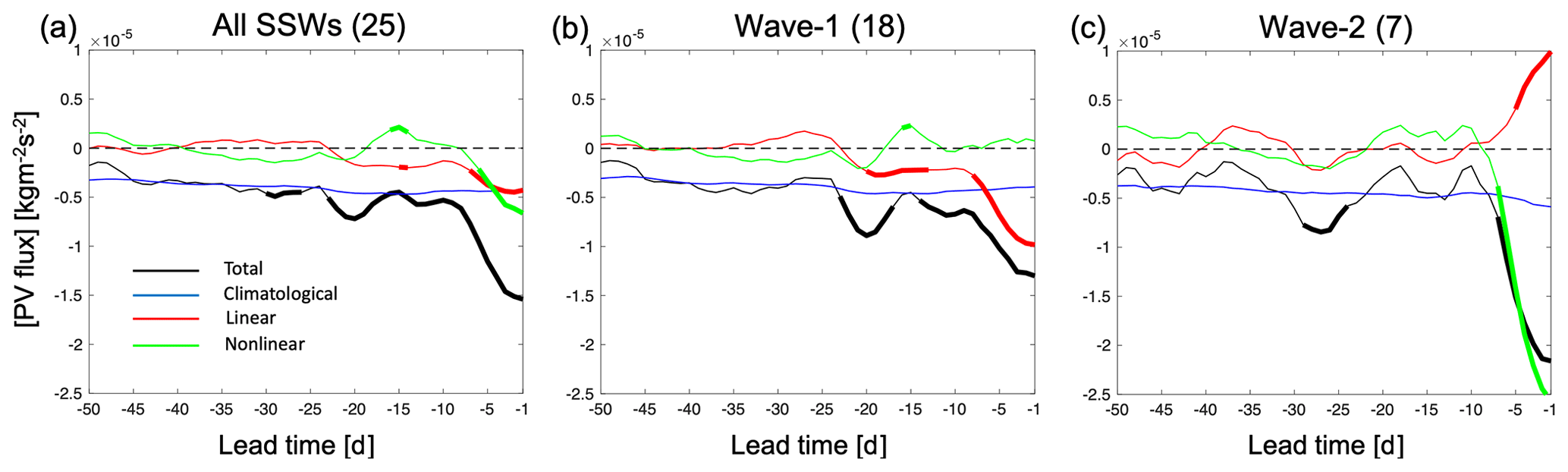
Figure 6Composites of zonal-mean poleward PV flux averaged north of 45∘ N and its decomposition in Eq. (11) as a function of lead time before SSWs: (a) all SSW events, (b) wave-1 events, and (c) wave-2 events in ERA-Interim. A 5 d running mean is applied to all lines. Bold lines indicate the values that are outside the percentile range 2.5 to 97.5 of normal winter day values from bootstrapping as described in the text. Panels (a–c) all share the same color legend as (a).
As demonstrated in Sect. 2.4, the total linear and nonlinear advection terms in Eq. (5) are closely linked to the PV flux divergence, which offers a more intuitive interpretation in an Eulerian framework. In this section, we use ERA-Interim data to illustrate the physical interpretation of the increase in the linear and nonlinear advection terms in Eq. (5). The motivation to introduce the PV flux into the PV equation is that the zonal-mean PV flux is connected to the pseudo-divergence of the EP flux along isentropic surfaces and thus acts as the net eddy forcing term of the mean flow, thus allowing for connections with the theory of wave-mean flow interaction (i.e., Eqs. 6 and 10). According to McIntyre and Palmer (1983), the wave activity of planetary waves is converted to the angular momentum of the mean flow, which violates the non-acceleration condition (Charney and Drazin, 1961), leading to the reversal of the mean flow. To understand the importance of the zonal-mean PV flux during the development of SSWs, we decompose the zonal-mean PV flux into different components as in Ayarzagüena et al. (2011),
where the subscript “c” represents daily climatology, and “a” represents daily anomalies. On the right-hand side of Eq. (11), the first term corresponds to the climatological planetary waves, the second and third terms correspond to the interaction between the climatological planetary waves and the daily anomalies, and the fourth (last) term corresponds to the interaction between daily anomalies. Similar to Eq. (3), the second and third right-hand terms can be viewed as linear components and the fourth term as the nonlinear component. Figure 6 shows the composite of zonal-mean poleward PV flux averaged north of 45∘ N and its decomposition in Eq. (11) as a function of lead time ahead of SSW events. The first term on the right-hand side of Eq. (11) can be seen as a constant since its variation with time is very small as shown in Fig. 6. When approaching the onset day of SSWs, the zonal-mean PV flux (black) becomes increasingly negative, indicating a weakening of the polar vortex. This further decrease in the negative zonal-mean PV flux is mainly due to the linear interaction between the climatological planetary waves and the daily anomalies (red) and the nonlinear interaction between anomalies (green), which correspond to the total linear and nonlinear PV advection terms (right columns in Fig. 3), respectively. Even though the climatological planetary waves (blue) also have a negative contribution to the total PV flux, the variations are very small with time. Similar to the distinct contributions of the linear and nonlinear PV advection terms in the wave-1 and wave-2 SSW composites, the negative total zonal-mean PV flux is mainly due to its linear component in wave-1 SSWs (red in Fig. 6b) and its nonlinear component in wave-2 SSWs (green in Fig. 6c). The different behavior of the linear and nonlinear PV flux during different types of SSW events is consistent with the behavior of PV advection in Fig. 3 and is well aligned with the behavior of the vertical wave flux as shown in Figs. 7 and 8 of Smith and Kushner (2012). Different from Smith and Kushner (2012), the nonlinear (linear) component of the PV flux even becomes positive just before the onset of wave-1 (wave-2) events (the positive linear PV flux in wave-2 is statistically different from normal winter days), counteracting the weakening of the polar vortex. Similar behavior can also be found in the linear advection term for the wave-2 SSW composite (Fig. 3f). Even though the amplitude of the negative linear PV flux at around day −15 in the wave-2 SSW composite is small, it helps to weaken the polar vortex and to offset the effect induced by the positive nonlinear PV flux. Note that it is the meridional gradient of the poleward zonal-mean PV flux that is used to approximate the linear and nonlinear PV advection terms as demonstrated in Eq. (9). The poleward zonal-mean PV flux is proportional to the magnitude of its meridional gradient, and one can thus use it to approximate the linear and nonlinear advection terms and to provide a physical interpretation of the signals found in Sect. 3.
From Fig. 6, the linear and nonlinear zonal-mean PV fluxes emerge as potential indicators for the type of SSW events. Given the abrupt change of the PV flux in the 10 d, preceding the onset of the events, we next examine how the spatial patterns of the poleward PV flux lead to their distinct zonal-mean contributions in the two types of SSWs. Figure 7 shows the poleward linear and nonlinear PV flux horizontal patterns of the wave-1 and wave-2 composites. As shown in the previous analyses, the linear signals start to amplify at around 20–25 d preceding the onset of both types of SSWs, and later the nonlinear signals become the most important contributors to the breakdown of the vortex from day −10 onwards for wave-2 events, while the linear signals keep amplifying for wave-1 events. Based on the different behaviors of linear and nonlinear terms, the deceleration of the polar vortex can be separated into two different periods: the first period from around day −25 to day −15 and the second period from day −10 to day −1. Thus, two different lead times (day −15 and day −5) are displayed in Fig. 7 as an example to illustrate the spatial pattern of the PV flux in the two different periods before the onset of the events. The spatial patterns for the linear PV flux of wave-1 events are quasi-stationary from around day −20 (Fig. 7a and b). A similar wave-2 pattern is also shown in linear PV flux for wave-2 events in the period of 28 to 12 d preceding the onset date (Fig. 7c). This pattern disappears from day −11 (not shown), and the wave pattern shown in Fig. 7d develops continuously until the central day of the SSW event. At the same time the positive values of PV flux increase, leading to a positive zonal-mean PV flux when close to day 0. Different from the linear PV flux, the nonlinear PV flux shows a clearly higher wavenumber pattern in the second period of the development of wave-2 SSWs shown in Fig. 7h, which has a strongly negative PV flux over western North America and a strongly positive PV flux over eastern North America. The downwind growth of the PV flux reaches its minimum (negative anomalies) over the North Atlantic and shows positive anomalies over northern Europe. Then the PV flux gradually weakens downstream over northern Asia and the North Pacific. This organized wave pattern in the nonlinear PV flux does not emerge until day −11 and remains largely stationary until the onset of the wave-2 events. In the early stage of the warming (day −25 to day −15), the nonlinear PV flux has a very low magnitude as shown in Figure 7g. Since previous studies suggested that split SSWs have a predominantly barotropic structure (Manney et al., 1994; Matthewman et al., 2009; Albers and Birner, 2014), we investigate the vertical structure of the nonlinear PV flux in the wave-2 SSW composite. Figure 8b shows the longitude–height cross section of the nonlinear PV flux of the wave-2 SSW composite at day −5 as an example. As can be seen in Fig. 8b, the wave pattern shown in Fig. 7h extends throughout the stratosphere and displays barotropic characteristics for wave-2 events. On the other hand, the longitude–height cross section of the linear PV flux at day −5 of the wave-1 SSWs in Fig. 8a displays a more baroclinic structure in the Eurasia and Pacific regions. The spatial pattern of the nonlinear PV flux in the composite of wave-1 events exhibits substantial transient fluctuations without a clear wave pattern before day −9 (Fig. 7e) and shows a more stable and organized spatial pattern in the period from day −9 to day 0 (Fig. 7f). However, the magnitude of the nonlinear PV flux in wave-1 events is smaller than its linear flux counterpart and also smaller than the nonlinear PV flux in the wave-2 event composite.
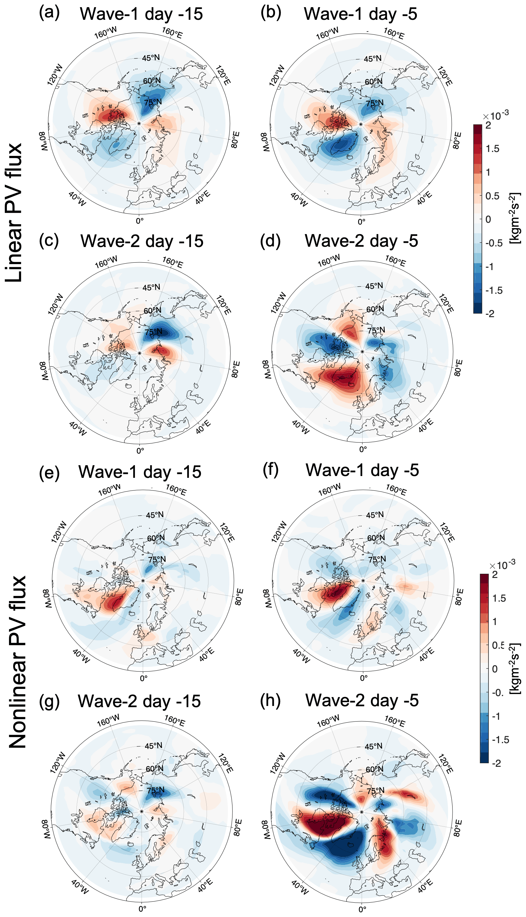
Figure 7The spatial pattern of the linear PV flux for (a, b) the composite of wave-1 SSWs and (c, d) the composite of wave-2 SSWs. The spatial pattern of the nonlinear PV flux for (e, f) the composite of wave-1 SSWs and (g, h) the composite of wave-2 SSWs. Panels (a, c, e, g) show the spatial pattern at day −15, and (b, d, f, h) show the spatial pattern at day −5 prior to the events.
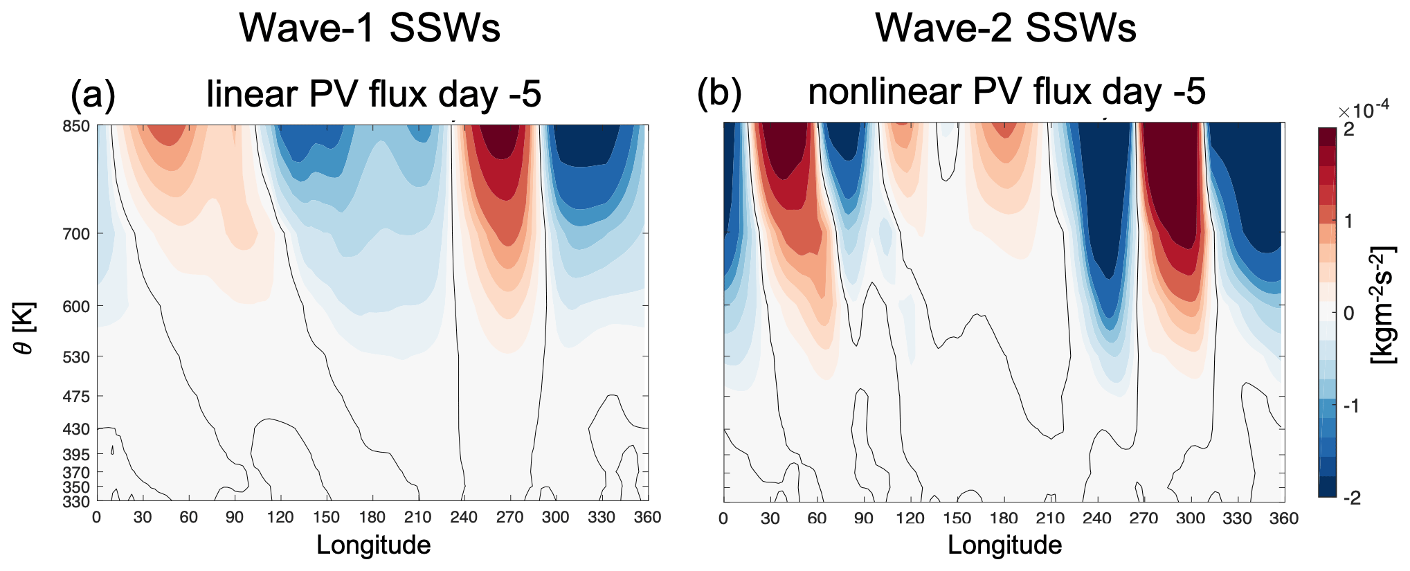
Figure 8The longitude–θ cross section of PV flux averaged north of 45∘ N at day −5. (a) Linear PV flux for wave-1 SSWs and (b) nonlinear PV flux for wave-2 SSWs. The black line indicates the zero value of PV flux.
Even though the spatial patterns of the linear PV flux in the two types of SSWs show a wave-2 pattern in the period of 20 to 10 d preceding the central day of SSWs, the locations of the maximum and minimum PV flux shift around 30∘ in longitude in the Pacific and North America regions (Fig. 7a and c). In the first period from day −10 to day 0, the wave pattern shown in Fig. 7h sets in and leads to the final split of the vortex for wave-2 SSWs. One relevant question is what processes lead to the differences observed in the evolution of the vortex breakdown where the linear PV flux remains important for wave-1 events, while the nonlinear PV flux amplifies for wave-2 events. Some previous studies suggested that the pre-SSW evolution of the polar vortex is distinct between split and displacement events (Charlton and Polvani, 2007; Bancalá et al., 2012), and this preconditioning could trigger the nonlinear resonance of planetary waves in the lower stratosphere, leading to the split of the polar vortex (Albers and Birner, 2014; Boljka and Birner, 2020). Here we examine the anomalies of PV and meridional wind after removing the daily climatology and zonal mean ( and , respectively; see Eq. 11) for the wave-1 and wave-2 events to understand their distinct evolutions after day −10. Figure 9a and b show the spatial pattern of (shading) and (green contour) at day −15 before wave-1 and wave-2 events, respectively. Both and present wave-1 patterns, but the positive and negative anomalies are located in different regions. The whole pattern of in wave-2 SSWs is around 60∘ further east compared to wave-1 SSWs. The negative is mainly located over eastern North America and the northern North Atlantic, which is important for the negative PV flux in the same region (Fig. 7a) for wave-1 SSWs, while for wave-2 SSWs the negative covers all of North America. These differences in the location of (shading) and (green contour) between the two types of SSW events are amplified from day −10 (Fig. 9c–d). The magnitudes of and in the first period from day −10 to day 0 are larger than in the second period from day −25 to day −15. The negative is located more over North America, while the positive is located over the North Atlantic and Europe for wave-1 SSWs (Fig. 9c). For wave-2 SSWs, the pattern of is the opposite (Fig. 9d). The positive extends to the full North Pacific (Fig. 9c), and both and maintain wave-1 structure for wave-1 SSWs. In contrast, (Fig. 9d) develops a wave-2 structure from day −10 onwards for wave-2 events. The weak positive over Asia (Fig. 9d) further develops from day −5, resulting in a wave-2 structure over midlatitude at day 0 (not shown). The main features of nonlinear PV flux in Fig. 7 can be roughly inferred by and in Fig. 9. We note that the composite of the nonlinear PV flux term is not equal to the direct product of the composites of and , and thus some features in Fig. 7 cannot be directly inferred from Fig. 9. We also find that the nonlinear PV flux and the and form a positive feedback from around day −10 to the onset of the wave-2 events. As the amplitude of and becomes larger, the nonlinear PV flux is also amplified, particularly in the region of the negative nonlinear PV flux over western North America and the North Atlantic as shown in Fig. 7h. The strong negative nonlinear PV flux contributes to more negative net zonal-mean PV flux values, suggesting a zonal-mean EP flux convergence. This EP flux convergence thus further decelerates the polar vortex. According to the non-acceleration theorem (Charney and Drazin, 1961), the deceleration of the polar vortex is accompanied by stronger wave activity, which is represented by the increasing amplitude of and . We also note that the spatial pattern of in Fig. 9f finally leads to the split of the polar vortex in wave-2 events, with the positive values corresponding to one of the daughter vortices located around 60∘ W.
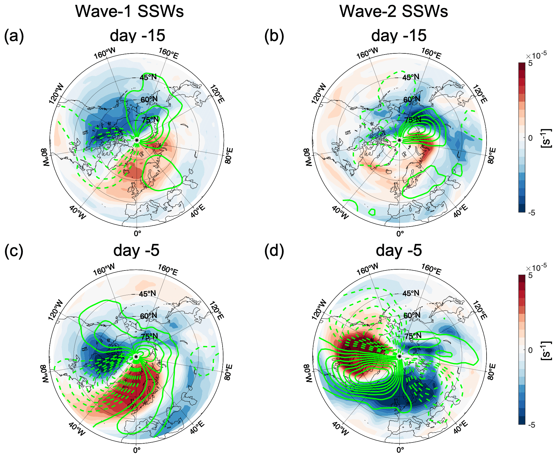
Figure 9The spatial pattern of anomalies of PV and meridional wind after removing the daily climatology and zonal mean values (a, b) on day −15 and (c, d) on day −5. Panels (a, c) show the composites of wave-1 SSWs, and (b, d) show the composites of wave-2 SSWs. Shading is for the PV anomalies (), and the green contour is for the meridional wind anomalies () with dashes for negative values. The contour interval of is 10 m s−1.
In this paper we employ a mode decomposition analysis to investigate the preconditioning of sudden stratospheric warming events. We study the (linear and nonlinear) terms in the potential vorticity equation by means of a budget analysis in order to identify the components in the first PC time series A1 that allow us to distinguish the behavior of the polar vortex during SSW events from normal winter days. Moreover, we identify characteristics of SSWs that help to identify the type of event (wave-1 vs. wave-2) during the dynamical development of SSWs. The mode decomposition analysis allows us to obtain a mode equation budget that describes the temporal evolution of the stratospheric dynamical processes that lead to the breakdown of the polar vortex. A better understanding of the vortex weakening process may help to improve the predictability of SSW events. The rate of change of the first PC time series represents the evolution of the strength of the polar vortex, and we find a significant increase in at around 25 d before the onset of SSWs. This change in marks the start of the vortex weakening process, indicating an acceleration of the polar vortex breakdown, and is different from the evolution of during normal winter days. The lead time of 25 d that we identified in our analysis is far beyond the current predictability limit of SSW events (Domeisen et al., 2020a). We note that not only the composite of SSWs, but also most of the individual SSW events show the increase in at around 20–25 d before the onset. The increase in is mainly due to the increase in the linear PV advection term, which preconditions the weakening of the polar vortex. While recent work suggests that split SSW events are less predictable than displacement events (Taguchi, 2018; Domeisen et al., 2020a), the preconditioning by the increase in the linear PV advection and PV flux is important for both wave-1 and wave-2 SSW events at around 20 d before the onset of the event, implying a similar intrinsic predictable timescale with 20 d lead for both types of events. From around 10 d before the events, the nonlinear PV advection term increases rapidly for wave-2 SSWs, but it remains small for wave-1 SSWs. As the nonlinear PV advection term increases, the linear PV advection drops dramatically prior to wave-2 SSWs. The distinct behavior of the linear and nonlinear advection terms in this 10 d period suggests that the type of SSW event could be inferred at around 10 d to 1 week prior to the events. Note that the type of event is determined by the larger wavenumber component of eddy heat flux in the period of −2 to 0 d before the events, and hence the 10 d lead times need to be interpreted with caution. The above differences are also present in the displacement and split SSW events, but the differences are somewhat smaller than those between wave-1 and wave-2 events, as not all split events are induced by wave-2 planetary waves.
Even though the contributions from linear and nonlinear PV advection terms are different in the two types of SSW events, their overall effects on within 10 d before the events are the same, causing to increase abruptly. The breakdown of the polar vortex can be divided into two periods based on the different behavior of the linear and nonlinear terms. During the first period, i.e., from 25 d to 2 weeks before the onset of SSWs, the linear term weakens the polar vortex for both types of SSWs, and during the second period, i.e., from around 10 d before the onset date until the onset, the vortex evolution for both types of SSWs starts to diverge, and the distinct vortex breakdown structures gradually develop. These two different time periods before the onset of the events are consistent with previous studies, especially for wave-2 SSWs (Labitzke, 1981; Bancalá et al., 2012; Albers and Birner, 2014), which suggested that an amplification of the wave-1 component allows the wave-2 wave flux to grow and propagate more effectively into the already weakening polar vortex region.
In both the ERA-Interim reanalysis and the simplified Isca model experiments, the increase in is more abrupt for wave-2 SSW events than for wave-1 events and thus results in a larger in the 10 d period preceding the onset of the events. The abrupt changes in are mainly due to the exponential increase in the nonlinear PV advection term. By contrast, the linear PV advection for wave-1 SSWs increases more slowly but consistently. The rapid growth of the nonlinear process for wave-2 SSWs could be related to a positive feedback between the nonlinear PV flux and the anomalies of PV and meridional wind when we tried to interpret the underlying dynamics of the increase in the nonlinear PV advection obtained from the mode equation budget. The linear and nonlinear advection terms are closely linked to the PV flux divergence, while the zonal-mean PV flux can be directly related to the zonal mean momentum budget (McIntyre and Palmer, 1983; Tung, 1986; Plumb, 2010). The zonal-mean poleward PV flux can be further decomposed into the linear and nonlinear components, whose role in the weakening of the polar vortex is similar to the effect of the PV advection terms on the increase in . The wave-2 spatial pattern of the linear PV flux helps to precondition the stratospheric basic state and decelerate the polar vortex in the first period of the SSW development for both types of SSWs. When the vortex weakening process evolves to the second period, the evolution of the PV flux for the two types of SSW events bifurcates as the linear and nonlinear PV fluxes exclusively amplify in the wave-1 and wave-2 events, respectively. This bifurcation could be due to the specific evolution of the stratospheric states in the two types of events (Charlton and Polvani, 2007; Albers and Birner, 2014), which can be seen from the horizontal patterns of the PV and meridional wind zonal anomalies. Our results suggest that the high wavenumber pattern that emerged in the second period for wave-2 SSWs is closely connected to the wave-2 wave flux and could be essential to the split of the vortex.
As suggested by Aikawa et al. (2019), mode decomposition analysis allows us to investigate the contribution of each EOF mode to the breakdown of the polar vortex and the way the associated spatial patterns play a role in the temporal evolution of the first PC time series. We found that the interactions involving the low modes are the dominant contributors to the weakening of the polar vortex, especially for the increase in the linear advection term in the first period (i.e., day −25 to day −15). Further investigation of the contribution from each EOF mode to the linear and nonlinear advection terms in the mode equation budget suggests that the increase in the linear advection term in the first period is largely influenced by the second and third EOF modes, which both show a wave-1 structure. The first EOF mode only plays an important role at around 1 week before the SSW event, suggesting that the process for the vortex weakening is initiated by modes that are not zonally symmetric. In terms of the nonlinear advection terms, the interactions amongst the first five EOF modes are important when approaching the onset of SSWs.
Even though the increase in and the contribution from the linear term start at around 25–20 d before the onset of SSWs in ERA-Interim, one needs to be cautious about the interpretation. The signals shown in the composite of SSWs do not necessarily indicate that these signals can be used to predict each individual SSW event with lead times of 20–25 d. While most SSW events do show a consistent positive starting 20 d before the SSW onset, around 30 % of all SSWs in ERA-Interim do not show this clear increase in around lead times of 20–25 d. On the other hand, the linear signals found here with lead times of 3–4 weeks may not be exclusive to SSWs. There are cases where large positive values of the first PC time series do not correspond to an SSW event but instead to a strong deceleration event. However, and the contribution from its linear term for SSW events are overall stronger and more persistent than that for the strong deceleration events (not shown). What we found here suggests that the intrinsic predictability of SSWs may be longer than the current 2-week practical predictability. However, more work is still needed to investigate whether the practical predictability of SSWs can actually be extended and if so then how.
Since the signals shown here indicate that most SSWs may be predictable on subseasonal timescales, it is important to understand which processes lead to the variability of the first EOF pattern and help to improve subseasonal forecast skill. A recent study by Albers and Newman (2021) identified two modes that relate to the linear and nonlinear processes for strong downward-propagating stratospheric anomalies, with one mode representing purely stratospheric processes and the other mode representing stratosphere–troposphere coupling. However, they point out that it is not clear which processes are more important for subseasonal predictability. Even though we have not connected the specific physical processes to the linear and nonlinear signals that are important for the two types of SSWs in this study, the spatial patterns of the PV flux could potentially provide some hints for future investigation. For example, the wave-2 spatial patterns of the linear PV flux are relatively stationary for wave-1 SSW events. This is due to the fact that the orientation of the negative and positive anomalies does not change significantly from day −19 onwards and the orientation of the wave-1 structure also remains stationary in both PV and meridional wind anomalies. These persistent spatial patterns and the linear behavior in the early stage of development of SSWs may be related to weather phenomena, such as blocking, teleconnections, and low-frequency modes in the troposphere. For example, Smith and Kushner (2012) and Cohen and Jones (2011) suggested that displacement events are preceded by sea level pressure anomalies associated with the Siberian high, which is consistent with the increase in linear vertical wave flux before the events.
In conclusion, our study finds signals that are representative of SSW events as early as 25 d preceding the events. This lead time is significantly longer than the current predictability limit of SSWs. We furthermore find that mode decomposition analysis can help infer wave-1 and wave-2 events at least 1 week ahead of the event, which is longer than the lead times identified in previous studies (Karpechko, 2018; Taguchi, 2018; Domeisen et al., 2020a). The timescale of emergence of the distinct evolution between linear and nonlinear terms provides insights into the different dynamical processes responsible for the two types of SSWs and thus could be potentially used as a predictor of the type of event in future studies. The fact that the noticeable increase in in the simplified general circulation model (GCM) (Isca model) experiment, which directly indicates the weakening of the polar vortex, shows up only around 10 d before the onset of SSWs (i.e., at shorter lead times than for reanalysis) suggests that the observed atmosphere tends to be more predictable than the model, which agrees with theory (Smith et al., 2016; Scaife and Smith, 2018). Applying the mode decomposition analysis to more complex forecasting models, i.e., S2S reforecast models (Vitart et al., 2017), to examine the predictability of SSWs will provide further insights into the dynamics of the polar vortex weakening and might potentially allow for the prediction of these events beyond the current lead times.
In this appendix, we show the derivation procedure for obtaining the mode decomposition equation budget (Eq. 4) and the cumulative explained variance and the power spectrum of the first 1000 EOF modes. The spatial patterns associated with the projections (U1, U2, …, Ud) of the wind vector daily anomalies Va onto the PC time series are computed by projecting Va onto the PC time series ({A1, A2, …, Ad}). Note that U1, U2, …, Ud are not necessarily orthogonal. The anomaly terms of PV and the wind vector fields can be written as
By substituting Eq. (A1) into Eq. (3), we get
Taking the inner product between Eq. (A3) and a given EOF mode Ek, we obtain
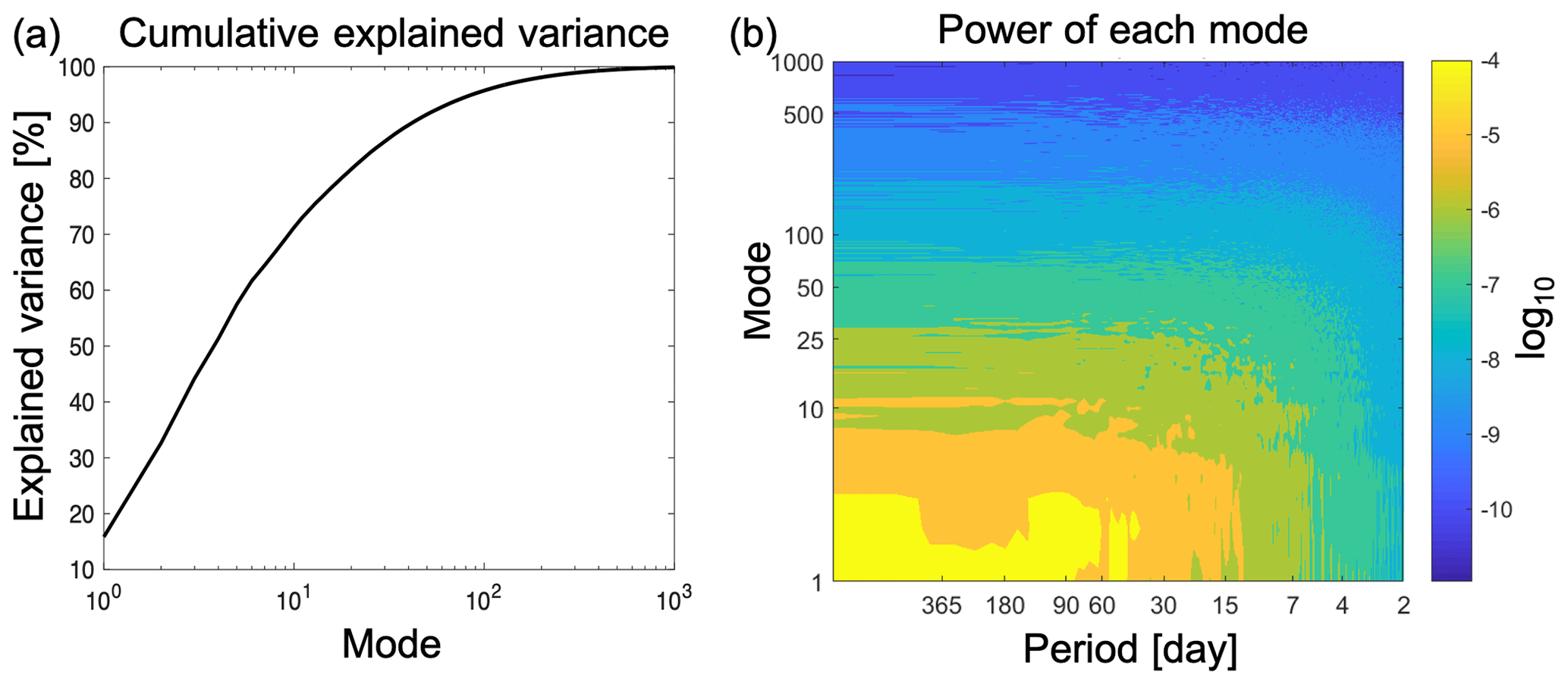
Figure A1(a) The cumulative explained variance of the first 1000 EOF modes of PV. (b) The power spectrum of the first 1000 EOF modes.
Given that {A1, A2, …, Ad} form an orthogonal basis, i.e., for a given mode k (with δkn=1 for n=k, and δkn=0 for n≠k), with Ck being the eigenvalue of mode k, the mode equation budget is computed as
which is the expression of Eq. (4) in Sect. 2.2.
Here we show the justification for the choice of truncation at the 1000th EOF mode and the choice of low modes. The first 1000 modes together explain ≈100 % of the variance of the PV anomalies of all winter days in ERA-Interim. The powers of the first 25 EOF modes are concentrated in the period longer than 1 week. Therefore, we defined mode 1–25 as low modes.
In this appendix, we show the derivation for obtaining approximations of the linear and nonlinear terms (Eq. 9) in the A1 tendency equation using the PV flux form. Taking the inner product between Eq. (8) and E1, and neglecting the variation in in the inner products, we obtain the following approximation of the rate of change of A1:
where C1 is the eigenvalue associated with the first EOF mode of PV. Comparing the linear and nonlinear terms in Eq. (B1) with those in Eq. (A4), we can see that
As we mentioned in Sect. 2.3, given the wavenumber-0 structure of E1, we further approximate E1 to be only a function of latitude. Thus, taking the inner product with E1 can be approximated as taking a latitude-weighted integral of the meridional gradient of PV flux as demonstrated below:
where a is the radius of the Earth, and ϕ is the latitude with ϕ1=30∘ N and ϕ2=90∘ N. Using Eq. (B3), we can obtain the approximated linear and nonlinear terms from Eq. (9).
In this appendix, we show the spatial patterns of the first 10 EOF modes of PV anomalies at 850 K and the associated first PC time series in the Isca model as described in Sect. 2.1. The first 10 modes together explain ≈82 % of the variance of the PV anomalies of all winter days in the Isca model.
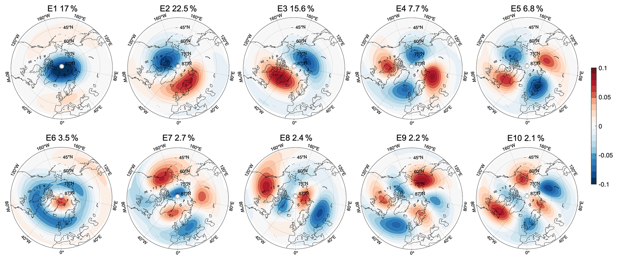
Figure C1The first 10 EOF modes of PV at 850 K (E1, E2, …, E10) of the combined set of basis vectors as described in Sect. 2.1 using the simplified Isca model daily data. The percentage number indicates the variance explained by each EOF.
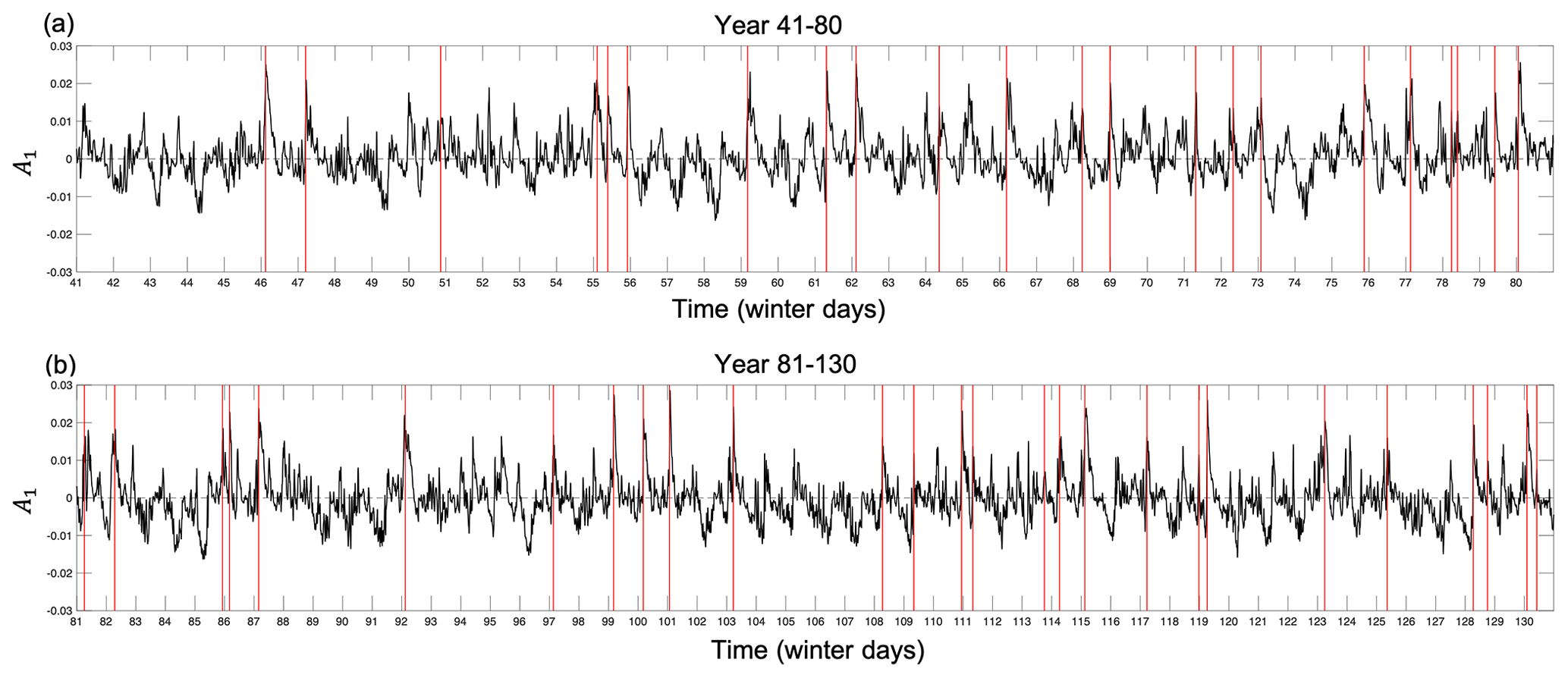
Figure C2The PC time series (A1) of winter days corresponding to the first EOF spatial pattern (E1) using daily Isca model winter data (from October to April) for the (a) years 41–80 and (b) years 81–130. The PC time series for the winter days of the years 1–40 can be seen in Fig. 2b. The red lines indicate the onset dates of SSW events.
In this appendix, we show the A1 mode decomposition budget for the composites of displacement and split SSW events in ERA-Interim, which can be compared with Fig. 3.
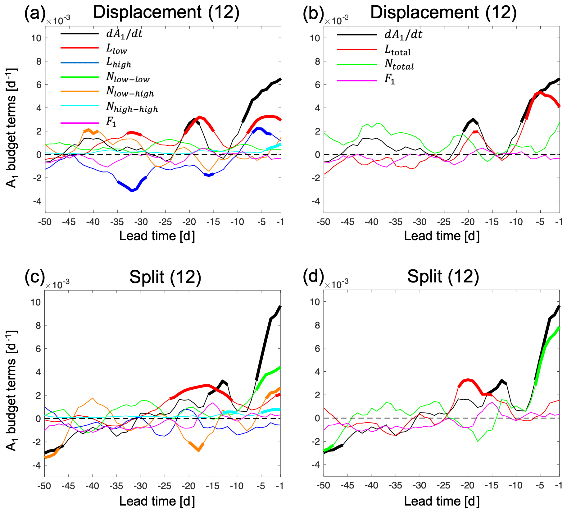
Figure D1The composite of the A1 budget as a function of lead time from 50 to 1 d before the onset of events in ERA-Interim. (a, b) Composite of displacement events; (c, d) composite of split events. Panels (a, c) show each term of the mode equation budget (Eq. 5) separately, and (b, d) show the sum of the linear and nonlinear terms for the two types of events. The number in the bracket in each panel title indicates the number of SSW events. A 5 d running mean is applied to all lines. Bold lines indicate the values that are outside the percentile range 2.5 to 97.5 of normal winter day values from bootstrapping as described in the text. The representation of each line color in (c) and (d) is the same as the legend in (a) and (b), respectively.
The Isca modeling framework was downloaded from the GitHub repository (https://github.com/ ExeClim/Isca, last access: May 2020) (Vallis et al., 2018)). ERA-Interim reanalysis (Dee et al., 2011) was obtained from the ECMWF server (https://apps.ecmwf.int/datasets/data/interim-full-daily, last access: May 2020).
ZW performed the derivations and data analysis, made the figures, and wrote the first draft. BJE performed the Isca model computations. ZW and DIVD designed and supervised the study. All authors provided feedback for the manuscript and helped with discussions of the analysis.
The authors declare that they have no conflict of interest.
Publisher's note: Copernicus Publications remains neutral with regard to jurisdictional claims in published maps and institutional affiliations.
The work of Zheng Wu and Raphaël de Fondeville was funded by the Swiss Data Science Center within the project EXPECT (C18-08). Funding from the Swiss National Science Foundation to Bernat Jiménez-Esteve and Daniela I. V. Domeisen through project PP00P2_170523 is gratefully acknowledged. This project has received funding from the European Research Council (ERC) under the European Union's Horizon 2020 research and innovation program (grant agreement no. 847456). The authors would like to thank the two anonymous reviewers, John Albers, and the co-editor Thomas Birner for their helpful comments throughout the revision of the manuscript.
This research has been supported by the Schweizerischer Nationalfonds zur Förderung der Wissenschaftlichen Forschung (grant no. PP00P2_170523), the Swiss Data Science Center (project no. C18-08), and the European Research Council (grant no. 847456).
This paper was edited by Thomas Birner and reviewed by two anonymous referees.
Aikawa, T., Inatsu, M., Nakano, N., and Iwano, T.: Mode-decomposed equation diagnosis for atmospheric blocking development, J. Atmos. Sci., 76, 3151–3167, https://doi.org/10.1175/JAS-D-18-0362.1, 2019. a, b, c, d, e
Albers, J. R. and Birner, T.: Vortex preconditioning due to planetary and gravity waves prior to sudden stratospheric warmings, J. Atmos. Sci., 71, 4028–4054, https://doi.org/10.1175/JAS-D-14-0026.1, 2014. a, b, c, d, e, f, g
Albers, J. R. and Newman, M.: Subseasonal predictability of the North Atlantic Oscillation, Environ. Res. Lett., 16, 2021, https://doi.org/10.1088/1748-9326/abe781, 2021. a
Ayarzagüena, B., Langematz, U., and Serrano, E.: Tropospheric forcing of the stratosphere: A comparative study of the two different major stratospheric warmings in 2009 and 2010, J. Geophys. Res., 116, D18114, https://doi.org/10.1029/2010JD015023, 2011. a
Ayarzagüena, B., Polvani, L. M., Langematz, U., Akiyoshi, H., Bekki, S., Butchart, N., Dameris, M., Deushi, M., Hardiman, S. C., Jöckel, P., Klekociuk, A., Marchand, M., Michou, M., Morgenstern, O., O'Connor, F. M., Oman, L. D., Plummer, D. A., Revell, L., Rozanov, E., Saint-Martin, D., Scinocca, J., Stenke, A., Stone, K., Yamashita, Y., Yoshida, K., and Zeng, G.: No robust evidence of future changes in major stratospheric sudden warmings: a multi-model assessment from CCMI, Atmos. Chem. Phys., 18, 11277–11287, https://doi.org/10.5194/acp-18-11277-2018, 2018. a
Ayarzagüena, B., Palmeiro, F. M., Barriopedro, D., Calvo, N., Langematz, U., and Shibata, K.: On the representation of major stratospheric warmings in reanalyses, Atmos. Chem. Phys., 19, 9469–9484, https://doi.org/10.5194/acp-19-9469-2019, 2019. a
Baldwin, M. P. and Dunkerton, T. J.: Stratospheric harbingers of anomalous weather regimes, Science, 294, 581–584, https://doi.org/10.1126/science.1063315, 2001. a, b
Baldwin, M. P., Ayarzagüena, B., Birner, T., Butchart, N., Butler, A. H., Charlton‐Perez, A. J., Domeisen, D. I. V., Garfinkel, C. I., Garny, H., Gerber, E. P., Hegglin, M. I., Langematz, U., and Pedatella, N. M.: Sudden Stratospheric Warmings, Rev. Geophys., 59, 1–37, https://doi.org/10.1029/2020rg000708, 2021. a
Bancalá, S., Krüger, K., and Giorgetta, M.: The preconditioning of major sudden stratospheric warmings, J. Geophys. Res.-Atmos., 117, 1–12, https://doi.org/10.1029/2011JD016769, 2012. a, b, c, d, e, f, g, h, i, j
Betts, A. K. and Miller, M. J.: A new convective adjustment scheme. Part II: Single column tests using GATE wave, BOMEX, ATEX and arctic air-mass data sets, Q. J. Roy. Meteorol. Soc., 112, 693–709, https://doi.org/10.1002/qj.49711247308, 1986. a
Birner, T. and Albers, J. R.: Sudden stratospheric warmings and anomalous upward wave activity flux, Scient. Onl. Lett. Atmos., 13, 8–12, https://doi.org/10.2151/sola.13A-002, 2017. a
Blume, C., Matthes, K., and Horenko, I.: Supervised learning approaches to classify sudden stratospheric warming events, J. Atmos. Sci., 69, 1824–1840, https://doi.org/10.1175/JAS-D-11-0194.1, 2012. a
Boljka, L. and Birner, T.: Tropopause-level planetary wave source and its role in two-way troposphere–stratosphere coupling, Weather Clim. Dynam., 1, 555—575, https://doi.org/10.5194/wcd-1-555-2020, 2020. a
Butler, A. H., Seidel, D. J., Hardiman, S. C., Butchart, N., Birner, T., and Match, A.: Defining sudden stratospheric warmings, B. Am. Meteorol. Soc., 96, 1913–1928, https://doi.org/10.1175/BAMS-D-13-00173.1, 2015. a
Charlton, A. J. and Polvani, L. M.: A New Look at Stratospheric Sudden Warmings. Part I: Climatology and Modeling Benchmarks, J. Climate, 20, 449–469, https://doi.org/10.1175/JCLI3994.1, 2007. a, b, c, d, e, f, g, h
Charney, J. G. and Drazin, P.: Propagation of Planetary-Scale Disturbances from the Lower into the Upper Atmosphere, J. Geophys. Res., 66, 83–109, https://doi.org/10.1029/JZ066i001p00083, 1961. a, b, c
Charney, J. G. and Eliassen, A.: A Numerical Method for Predicting the Perturbations of the Middle Latitude Westerlies, Tellus, 1, 38–54, https://doi.org/10.3402/tellusa.v1i2.8500, 1949. a
Cohen, J. and Jones, J.: Tropospheric precursors and stratospheric warmings, J. Climate, 24, 6562–6572, https://doi.org/10.1175/2011JCLI4160.1, 2011. a
Dee, D. P., Uppala, S. M., Simmons, A. J., Berrisford, P., Poli, P., Kobayashi, S., Andrae, U., Balmaseda, M. A., Balsamo, G., Bauer, P., Bechtold, P., Beljaars, A. C., van de Berg, L., Bidlot, J., Bormann, N., Delsol, C., Dragani, R., Fuentes, M., Geer, A. J., Haimberger, L., Healy, S. B., Hersbach, H., Hólm, E. V., Isaksen, L., Kållberg, P., Köhler, M., Matricardi, M., Mcnally, A. P., Monge-Sanz, B. M., Morcrette, J. J., Park, B. K., Peubey, C., de Rosnay, P., Tavolato, C., Thépaut, J. N., and Vitart, F.: The ERA-Interim reanalysis: Configuration and performance of the data assimilation system, Q. J. Roy. Meteorol. Soc., 137, 553–597, https://doi.org/10.1002/qj.828, 2011. a, b
de la Cámara, A., Birner, T., and Albers, J. R.: Are sudden stratospheric warmings preceded by anomalous tropospheric wave activity?, J. Climate, 32, 7173–7189, https://doi.org/10.1175/JCLI-D-19-0269.1, 2019. a
Domeisen, D. I. V.: Estimating the Frequency of Sudden Stratospheric Warming Events From Surface Observations of the North Atlantic Oscillation, J. Geophys. Res.-Atmos., 124, 3180–3194, https://doi.org/10.1029/2018JD030077, 2019. a, b
Domeisen, D. I. V. and Plumb, A. R.: Traveling planetary-scale Rossby waves in the winter stratosphere: The role of tropospheric baroclinic instability, Geophys. Res. Lett., 39, 1–5, https://doi.org/10.1029/2012GL053684, 2012. a
Domeisen, D. I. V., Butler, A. H., Charlton-Perez, A. J., Ayarzagüena, B., Baldwin, M. P., Dunn-Sigouin, E., Furtado, J. C., Garfinkel, C. I., Hitchcock, P., Karpechko, A. Y., Kim, H., Knight, J., Lang, A. L., Lim, E. P., Marshall, A., Roff, G., Schwartz, C., Simpson, I. R., Son, S. W., and Taguchi, M.: The Role of the Stratosphere in Subseasonal to Seasonal Prediction: 1. Predictability of the Stratosphere, J. Geophys. Res.-Atmos., 125, 1–17, https://doi.org/10.1029/2019JD030920, 2020a. a, b, c, d, e
Domeisen, D. I. V., Butler, A. H., Charlton-Perez, A. J., Ayarzagüena, B., Baldwin, M. P., Dunn-Sigouin, E., Furtado, J. C., Garfinkel, C. I., Hitchcock, P., Karpechko, A. Y., Kim, H., Knight, J., Lang, A. L., Lim, E. P., Marshall, A., Roff, G., Schwartz, C., Simpson, I. R., Son, S. W., and Taguchi, M.: The Role of the Stratosphere in Subseasonal to Seasonal Prediction: 2. Predictability of the Stratosphere, J. Geophys. Res.-Atmos. 125, 1–20, https://doi.org/10.1029/2019JD030923, 2020b. a
Dommenget, D. and Latif, M.: A cautionary note on the interpretation of EOFs, J. Climate, 15, 216–225, https://doi.org/10.1175/1520-0442(2002)015<0216:ACNOTI>2.0.CO;2, 2002. a
Edmon, H. J., Hoskins, B. J., and McIntyre, M. E.: Eliassen-Palm Cross Sections for the Troposphere, J. Atmos. Sci., 37, 2600–2616, https://doi.org/10.1175/1520-0469(1980)037<2600:EPCSFT>2.0.CO;2, 1981. a
Esler, J. G. and Matthewman, N. J.: Stratospheric sudden warmings as self-tuning resonances. Part II: Vortex displacement events, J. Atmos. Sci., 68, 2505–2523, https://doi.org/10.1175/JAS-D-11-08.1, 2011. a
Gerber, E. . and Polvani, L. M.: Stratosphere-Troposphere Coupling in a Relatively Simple AGCM: The Importance of Stratospheric Variability, J. Climate, 22, 1920–1933, 2009. a
Held, I. M., Ting, M., and Wang, H.: Northern winter stationary waves: Theory and modeling, J. Climate, 15, 2125–2144, https://doi.org/10.1175/1520-0442(2002)015<2125:NWSWTA>2.0.CO;2, 2002. a
Hitchcock, P. and Haynes, P. H.: Stratospheric control of planetary waves, Geophys. Res. Lett., 43, 884–11, https://doi.org/10.1002/2016GL071372, 2016. a
Hoskins, B. J., McIntyre, M. E., and Robertson, A. W.: On the use and significance of isentropic potential vorticity maps, Q. J. Roy. Meteorol. Soc., 111, 877–946, https://doi.org/10.1002/qj.49711147002, 1985. a
Jiménez-Esteve, B. and Domeisen, D. I. V.: Nonlinearity in the North Pacific Atmospheric Response to a Linear ENSO Forcing, Geophys. Res. Lett., 46, 2271–2281, https://doi.org/10.1029/2018GL081226, 2019. a, b
Jucker, M.: Are Sudden Stratospheric Warmings Generic? Insights from an Idealized GCM, J. Atmos. Sci., 73, 5061–5080, https://doi.org/10.1175/JAS-D-15-0353.1, 2016. a
Jucker, M. and Reichler, T.: Dynamical Precursors for Statistical Prediction of Stratospheric Sudden Warming Events, Geophys. Res. Lett., 45, 13–124, https://doi.org/10.1029/2018GL080691, 2018. a
Karpechko, A. Y.: Predictability of sudden stratospheric warmings in the ECMWF extended-range forecast system, Mon. Weather Rev., 146, 1063–1075, https://doi.org/10.1175/MWR-D-17-0317.1, 2018. a
Karpechko, A. Y., Hitchcock, P., Peters, D. H. W., and Schneidereit, A.: Predictability of downward propagation of major sudden stratospheric warmings, Q. J. Roy. Meteorol. Soc., 60, 1459–1470, https://doi.org/10.1002/qj.3017, 2017. a, b
Kidston, J., Scaife, A. A., Hardiman, S. C., Mitchell, D. M., Butchart, N., Baldwin, M. P., and Gray, L. J.: Stratospheric influence on tropospheric jet streams, storm tracks and surface weather, Nat. Geosci., 8, 433–440, https://doi.org/10.1038/ngeo2424, 2015. a
King, A. D., Butler, A. H., Jucker, M., Earl, N. O., and Rudeva, I.: Observed Relationships Between Sudden Stratospheric Warmings and European Climate Extremes, J. Geophys. Res.-Atmos., 124, 13943–13961, https://doi.org/10.1029/2019JD030480, 2019. a
Kolstad, E. W., Breiteig, T., and Scaife, A. A.: The association between stratospheric weak polar vortex events and cold air outbreaks in the Northern Hemisphere, Q. J. Roy. Meteorol. Soc., 136, 886–893, https://doi.org/10.1002/qj.620, 2010. a
Labitzke, K.: Stratospheric-mesospheric midwinter disturbances: A summary of observed characteristics, J. Geophys. Res., 86, 9665, https://doi.org/10.1029/jc086ic10p09665, 1981. a, b
Limpasuvan, V., Thompson, D. W., and Hartmann, D. L.: The life cycle of the Northern Hemisphere sudden stratospheric warmings, J. Climate, 17, 2584–2596, https://doi.org/10.1175/1520-0442(2004)017<2584:TLCOTN>2.0.CO;2, 2004. a
Lindgren, E. A., Sheshadri, A., and Plumb, R. A.: Sudden Stratospheric Warming Formation in an Idealized General Circulation Model Using Three Types of Tropospheric Forcing, J. Geophys. Res.-Atmos., 123, 10–125, https://doi.org/10.1029/2018JD028537, 2018. a
Manney, G., Farrara, J., and Mechoso, C.: Simulations of the February 1979 Stratospheric Sudden Warming: Model Comparisons and Three-Dimensional Evolution, Mon. Weather Rev., 122, 1115–1140, 1994. a
Matsuno, T.: A Dynamical Model of the Stratospheric Sudden Warming, J. Atmos. Sci., 28, 1479–1494, https://doi.org/10.1175/1520-0469(1971)028<1479:ADMOTS>2.0.CO;2, 1971. a, b, c
Matthewman, N. J. and Esler, J. G.: Stratospheric sudden warmings as self-tuning resonances. Part I: Vortex splitting events, J. Atmos. Sci., 68, 2481–2504, https://doi.org/10.1175/JAS-D-11-07.1, 2011. a
Matthewman, N. J., Esler, J. G., Charlton-Perez, A. J., and Polvani, L. M.: A new look at stratospheric sudden warmings. Part III: Polar vortex evolution and vertical structure, J. Climate, 22, 1566–1585, https://doi.org/10.1175/2008JCLI2365.1, 2009. a, b, c
McIntyre, E.: How Well do we Understand the Dynamics of Stratospheric Warmings?, J. Meteorol. Soc. Jpn., 60, 37–65, https://doi.org/10.2151/jmsj1965.60.1_37, 1982. a, b
McIntyre, M. E. and Palmer, T.: Breaking planetary waves in the stratosphere, Nature, 305, 593–600, 1983. a, b
Mlawer, E. J., Taubman, S. J., Brown, P. D., Iacono, M. J., and Clough, S. A.: Radiative transfer for inhomogeneous atmospheres: RRTM, a validated correlated-k model for the longwave, J. Geophys. Res.-Atmos., 102, 16663–16682, https://doi.org/10.1029/97JD00237, 1997. a
Monahan, A. H., Fyfe, J. C., Ambaum, M. H., Stephenson, D. B., and North, G. R.: Empirical orthogonal functions: The medium is the message, J. Climate, 22, 6501–6514, https://doi.org/10.1175/2009JCLI3062.1, 2009. a
Mukougawa, H., Hirooka, T., and Kuroda, Y.: Influence of stratospheric circulation on the predictability of the tropospheric Northern Annular Mode, Geophys. Res. Lett., 36, L08814, https://doi.org/10.1029/2008GL037127, 2009. a
Nakagawa, K. I. and Yamazaki, K.: What kind of stratospheric sudden warming propagates to the troposphere?, Geophys. Res. Lett., 33, 3–6, https://doi.org/10.1029/2005GL024784, 2006. a, b
Plumb, R. A.: Planetary waves and the extratropical winter stratosphere, in: The Stratosphere: Dynamics, Transport, and Chemistry, Geophysical Monograph Series, 190, 23–41, https://doi.org/10.1029/2009GM000888, 2010. a
Polvani, L. M. and Waugh, D. W.: Upward wave activity flux as a precursor to extreme stratospheric events and subsequent anomalous surface weather regimes, J. Climate, 17, 3548–3554, https://doi.org/10.1175/1520-0442(2004)017<3548:UWAFAA>2.0.CO;2, 2004. a, b
Scaife, A. A. and Smith, D.: A signal-to-noise paradox in climate science, npj Clim. Atmos. Sci., 1, 1–8, https://doi.org/10.1038/s41612-018-0038-4, 2018. a
Scaife, A. A., Karpechko, A. Y., Baldwin, M. P., Brookshaw, A., Butler, A. H., Eade, R., Gordon, M., Maclachlan, C., Martin, N., Dunstone, N., and Smith, D.: Seasonal winter forecasts and the stratosphere, Atmos. Sci. Lett., 17, 51–56, https://doi.org/10.1002/asl.598, 2016. a
Scinocca, J. F. and Haynes, P. H.: Dynamical forcing of stratospheric planetary waves by tropospheric baroclinic eddies, J. Atmos. Sci., 55, 2361–2392, https://doi.org/10.1175/1520-0469(1998)055<2361:DFOSPW>2.0.CO;2, 1998. a
Sigmond, M., Scinocca, J. F., Kharin, V. V., and Shepherd, T. G.: Enhanced seasonal forecast skill following stratospheric sudden warmings, Nat. Geosci., 6, 98–102, https://doi.org/10.1038/ngeo1698, 2013. a
Smith, D. M., Scaife, A. A., Eade, R., and Knight, J. R.: Seasonal to decadal prediction of the winter North Atlantic Oscillation: Emerging capability and future prospects, Q. J. Roy. Meteorol. Soc., 142, 611–617, https://doi.org/10.1002/qj.2479, 2016. a
Smith, K. L. and Kushner, P. J.: Linear interference and the initiation of extratropical stratosphere-troposphere interactions, J. Geophys. Res.-Atmos., 117, 1–16, https://doi.org/10.1029/2012JD017587, 2012. a, b, c, d
Taguchi, M.: Comparison of Subseasonal-to-Seasonal Model Forecasts for Major Stratospheric Sudden Warmings, J. Geophys. Res.-Atmos., 123, 10231–10247, https://doi.org/10.1029/2018JD028755, 2018. a, b, c
Tung, K. K.: Nongeostrophic Theory of Zonally Averaged Circulation. Part I: Formulation, J. Atmos. Sci., 43, 2600–2618, 1986. a, b, c, d
Vallis, G. K., Colyer, G., Geen, R., Gerber, E., Jucker, M., Maher, P., Paterson, A., Pietschnig, M., Penn, J., and Thomson, S. I.: Isca, v1.0: A framework for the global modelling of the atmospheres of Earth and other planets at varying levels of complexity, Geosci. Model Dev., 11, 843–859, https://doi.org/10.5194/gmd-11-843-2018, 2018 (data available at: https://github.com/ ExeClim/Isca, last access: May 2020). a, b
Vitart, F., Ardilouze, C., Bonet, A., Brookshaw, A., Chen, M., Codorean, C., Déqué, M., Ferranti, L., Fucile, E., Fuentes, M., Hendon, H., Hodgson, J., Kang, H. S., Kumar, A., Lin, H., Liu, G., Liu, X., Malguzzi, P., Mallas, I., Manoussakis, M., Mastrangelo, D., MacLachlan, C., McLean, P., Minami, A., Mladek, R., Nakazawa, T., Najm, S., Nie, Y., Rixen, M., Robertson, A. W., Ruti, P., Sun, C., Takaya, Y., Tolstykh, M., Venuti, F., Waliser, D., Woolnough, S., Wu, T., Won, D.-J., Xiao, H., Zaripov, R., and Zhang, L.: The Subseasonal to Seasonal (S2S) Prediction Project Database, B. Am. Meteorol. Soc., 98, 163–173, 2017. a
Note that the sign of E1 is not important. Given the pattern of E1, the positive value of A1 corresponds to the weakening of the polar vortex and is an indication of a potential SSW event.
- Abstract
- Introduction
- Data and methodology
- Results of mode decomposition: mode equation budget
- Physical interpretation of the mode decomposition
- Conclusions
- Appendix A: Mode decomposition budget equation
- Appendix B: Relation between the rate of change of A1 and the PV flux
- Appendix C: EOF modes and PC time series of PV in the simplified Isca model
- Appendix D: Mode decomposition budget for displacement and split SSWs in ERA-Interim
- Code and data availability
- Author contributions
- Competing interests
- Disclaimer
- Acknowledgements
- Financial support
- Review statement
- References