Seasonal forecasts of the Saharan heat low characteristics: a multi-model assessment

The Saharan heat low (SHL) is a key component of the West African Monsoon system at the synoptic scale and a driver of summertime precipitation over the Sahel region. Therefore, accurate seasonal precipitation forecasts rely in part on a proper representation of the SHL characteristics in seasonal forecast models. This is investigated using the latest versions of two seasonal forecast systems namely the SEAS5 and MF7 systems from the European Center of Medium-Range Weather Forecasts (ECMWF) and Météo-France respectively. The SHL characteristics in the seasonal forecast models are assessed based on a comparison with the fifth ECMWF Reanalysis (ERA5) for the period 1993–2016. The analysis of the modes of variability shows that the seasonal forecast models have issues with the timing and the intensity of the SHL pulsations when compared to ERA5. SEAS5 and MF7 show a cool bias centered on the Sahara and a warm bias located in the eastern part of the Sahara respectively. Both models tend to underestimate the interannual variability in the SHL. Large discrepancies are found in the representation of extremes SHL events in the seasonal forecast models. These results are not linked to our choice of ERA5 as a reference, for we show robust coherence and high correlation between ERA5 and the Modern-Era Retrospective analysis for Research and Applications (MERRA). The use of statistical bias correction methods significantly reduces the bias in the seasonal forecast models and improves the yearly distribution of the SHL and the forecast scores. The results highlight the capacity of the models to represent the intraseasonal pulsations (the so-called east–west phases) of the SHL. We notice an overestimation of the occurrence of the SHL east phases in the models (SEAS5, MF7), while the SHL west phases are much better represented in MF7. In spite of an improvement in prediction score, the SHL-related forecast skills of the seasonal forecast models remain weak for specific variations for lead times beyond 1 month, requiring some adaptations. Moreover, the models show predictive skills at an intraseasonal timescale for shorter lead times.

1 Introduction

In the Sahel region, food security for populations depends on rainfed agriculture which is conditioned by seasonal rainfall (Durand, 1977; Bickle et al., 2020), characterized by a strong convective activity in the summer, associated with a large climatic variability (local- and large-scale forcings), generally leading to poor precipitation forecast skills at subseasonal and seasonal timescales in tropical North Africa (Vogel et al., 2018). Hence, climate models suffer from biases in the representation of West African Monsoon (WAM) processes and dynamics responsible for rainfall in West Africa (Roehrig et al., 2013; Martin et al., 2017). During the African Monsoon Multidisciplinary Analysis (AMMA) project (Redelsperger et al., 2006), the Saharan heat low (SHL) has been used as a key component to assess the variability in the WAM system. In particular, forecasters and researchers have pointed out the need to document the SHL predictability and its link with Sahelian rainfall (Janicot et al., 2008b). Improving precipitation forecasts not only is crucial for agriculture and water supply in the region but also is of paramount importance for floods and disease prevention.

The SHL refers to the low-surface-pressure area that appears above the Sahara region in the boreal summer due to seasonal high temperatures and insolation (e.g., Lavaysse et al., 2009). The SHL is an essential component of the WAM system at the synoptic scale (Sultan and Janicot, 2003; Parker et al., 2005; Peyrillé and Lafore, 2007; Lavaysse et al., 2009; Chauvin et al., 2010) and a driver of precipitation over the Sahel region (Lavaysse et al., 2010a; Evan et al., 2015). It plays an important role in the atmospheric circulation over West Africa and brings moisture from the Atlantic Ocean to the region, thereby favoring the installation of the monsoon flow. In the lower atmospheric layers, the cyclonic circulation generated by a strong SHL tends to reinforce the monsoon flow around its eastern flank and the Harmattan flow along the western flank (Lavaysse, 2015). In the mid-layers, the anticyclonic circulation associated with the divergent flow at the top of the SHL contributes to maintaining the African Easterly Jet (AEJ) at around 700 hPa and modulates its intensity (Thorncroft and Blackburn, 1999). An intensification of the AEJ is observed during strong phases of SHL activity (Lavaysse et al., 2010b). According to Lavaysse et al. (2009), the SHL maximum activity over the Sahara occurs on average from 20 June to 17 September, and it is located 20–30^∘ N, 7^∘ W–5^∘ E, covering much of northern Mauritania, Mali, Niger and southern Algeria (Fig. 1). The maximum of SHL activity happens during the rainfall season in the Sahel region (from June to September; Sultan and Janicot, 2003). The SHL is considered a reliable proxy for the regional- and large-scale forcings impacting the WAM (Lavaysse et al., 2010b).

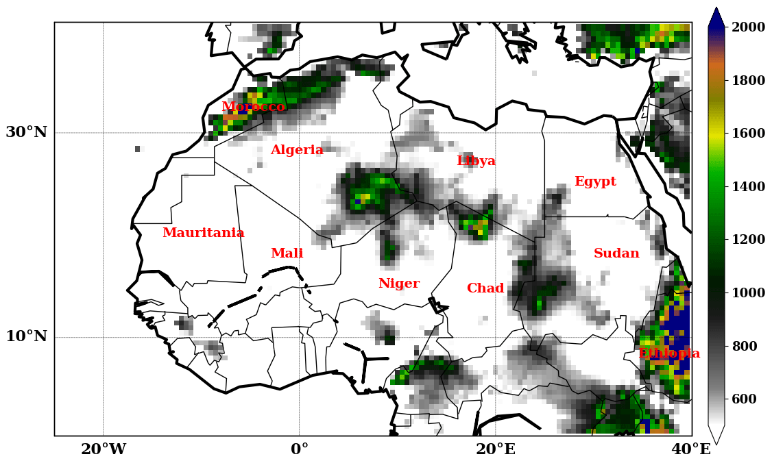
Figure 1 Topographic map of West Africa using ERA5 elevation data. The y axis and x axis represent the latitude and longitude respectively, in degrees over the domain. The color bar shows the elevation in meters over the region.

Lavaysse et al. (2009) monitored the seasonal evolution of the West African heat low (WAHL) using ERA-40 reanalyses and brightness temperature from the Cloud Archive User Service (CLAUS). They found a northwestward migration of the WAHL from a position south of the Darfur mountains in the winter to a location over the Sahara between the Hoggar and the Atlas mountains during the summer. They also estimated the climatological onset of the SHL occurring around 20 June (from the period 1984–2001) some days before the climatological monsoon onset date. This highlights strong links between the SHL and the monsoon flux. Chauvin et al. (2010) assessed the intraseasonal variability in the SHL and its link with midlatitudes using National Centers for Environmental Prediction (NCEP-2) reanalysis data. They found a robust mode of variability in the SHL over North Africa and the Mediterranean which can be decomposed into two phases called east–west oscillations. The west phase corresponds to a maximum temperature over the coast of Morocco–Mauritania, propagating southwestward, and a minimum temperature between Libya and Sicily, propagating southeastward. The east phase corresponds to the opposite temperature structure which propagates as in the west phase. Roehrig et al. (2011) studied the link between the variability in convection in the Sahel region and the variability in the SHL at an intraseasonal timescale using NCEP-2 reanalysis data. They showed that the onset of the monsoon is associated with strong SHL activity when the northerlies coming from the Mediterranean (sometimes called ventilation) are weak. Conversely, they revealed that the formation of a strong cold air surge over Libya and Egypt and its propagation toward the Sahel lead to the decrease in the SHL, which inhibits the WAM onset.

As detailed above, previous work has evidenced the importance and the role of the SHL in the West African climate. These studies are based on a climatological view of the SHL using mostly reanalysis data. One may legitimately wonder how seasonal forecast models represent the SHL evolution.

The seasonal forecast is a long-term forecast which is very useful because it allows an anticipation of seasonal trends. The use of an ensemble forecast for seasonal forecasting provides a range of forecasts and gives information about the spread associated with the forecast of a specific variable. Ensemble forecast models lead to an improvement in the predictive skills of some atmospheric variables (Haiden et al., 2015; Lavaysse et al., 2019). The evaluation of the SHL behavior in seasonal forecast models has not been addressed yet. Roehrig et al. (2013) show that the mean temperature over the Sahara from July to September is well correlated with rainfall position over the Sahel region. Provided that the SHL characteristics (i.e., the east and west pulsations of the heat low, its intensity, and its interannual variability) are well captured in seasonal forecast models simulations, they can be used as predictors for rainfall in the Sahel area.

The goal of this article is (i) to investigate the representation and the forecast skills of the SHL in two seasonal forecast models and (ii) to evaluate the added value of bias correction techniques on raw seasonal forecasts. Bias issues are very frequent in seasonal forecast models; by correcting them with statistical methods, the predictive skills of the models can be improved in order to provide atmospheric variables that better fit the characteristics of the observation.

To reach this aim, we firstly study the SHL variability modes in seasonal forecast models and reanalyses; secondly we estimate the biases between the forecasts and reanalyses. Finally, we assess the recent evolution of the SHL and proceed with an evaluation of forecasts with respect to the reanalyses.

The remainder of this article is organized as follows: in Sect. 2, we present our region of interest and the data used for this work; the description of the methodology adopted is also provided. Section 3 contains the main results of this investigation obtained by following the methodology described in Sect. 2. In Sect. 4, the predictive skills of the seasonal forecast models are discussed; and Sect. 5 provides a conclusion with some perspectives for future studies.

2 Data and methods

2.1 Saharan heat low evaluation metric

The location of the West African heat low has a strong seasonal variation: north–south owing to the seasonal cycle of insolation and east–west owing to orographic forcing (Lavaysse et al., 2009; Drobinski et al., 2005). It is termed SHL once it reaches its Saharan location generally within 20–30^∘ N, 7^∘ W–5^∘ E, during the monsoon season, an area that is bounded by the Atlas mountains to the north, the Hogar mountains to the east, the Atlantic Ocean to the west and the northern extent of the WAM to the south (Evan et al., 2015). The SHL has been detected in previous studies using the low-level atmospheric thickness (LLAT) computed as a geopotential distance between two pressure levels, 700 and 925 hPa (Lavaysse et al., 2009). Because the LLAT is due to a thermal dilatation of the low troposphere and in order to simplify the detection process, the SHL can be monitored by using the 850 hPa temperature field. Lavaysse et al. (2016) using ERA-Interim reanalysis, showed that the 850 hPa temperature (T850) field is well correlated to the LLAT and can be used as a proxy for the monitoring of the SHL (detection and intensity). As ERA5 is an improvement in ERA-Interim, we assume that the correlation between T850 and the LLAT is preserved in ERA5. We suppose this is also true for the forecast models. Consequently in this study, we use T850 to analyze the SHL characteristics. Because fixed boxes are used, the detection of the SHL is not needed, but strong (weak) phases of the SHL will be associated with high (low) T850.

2.2 Region of interest

The Sahara is located over 20–35^∘ N, 25^∘ W–40^∘ E, and covers large parts of Algeria, Chad, Egypt, Libya, Mali, Mauritania, Morocco, Niger, Western Sahara, Sudan and Tunisia (see topographic map in Fig. 1). The climate is associated with very hot temperatures from May to September of around 30 ^∘C for mean temperatures and over 40 ^∘C for mean maximum temperatures, very low humidity close to the surface (with relative humidities of less than 10 %), and a critical absence of rainfall.

It is also the region with the largest production of dust particles (Prospero et al., 2002). For this study, North Africa is subdivided in four regions (see Fig. 2) defined as follows:

• the Sahara area 20–30^∘ N, 10^∘ W–20^∘ E, and extending from the south of Morocco to Egypt;

• the central SHL here denoted as CSHL, located 20–30^∘ N, 7^∘ W–5^∘ E, and covering most of the north of Mauritania, Mali and the south of Algeria;

• the western SHL here denoted as WSHL, located 20–30^∘ N, 10–2^∘ W and including the north of Mauritania, Mali, the south of Morocco and Algeria;

• the eastern SHL denoted as ESHL, located 20–30^∘ N, 0–8^∘ E, and mostly in the south of Algeria.

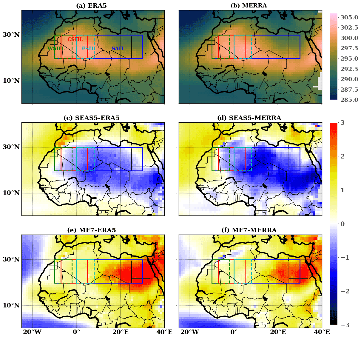
Figure 2 Climatology of the SHL during the JJAS period over 1993–2016 in the reanalysis data using T850, (a) ERA5 and (b) MERRA, and the anomalies of the climatologies of the SHL between (c) SEAS5 and ERA5, (e) SEAS5 and MERRA, (d) MF7 and ERA5, and (f) MF7 and MERRA. The rectangles indicate the boxes chosen for the computation of the average T850 and their corresponding name. WSHL: western SHL; CSHL: central SHL; ESHL: eastern SHL; SAH: the Saharan region. The color bars indicate T850 (a, b) and the anomalies of T850 (c–f) in kelvins. The computation was made using the ensemble mean member.

The choice of the four regions is supported by previous studies: Lavaysse et al. (2009) highlight a maximum activity of the SHL in the CSHL location during summer (JJAS period, June–September); Roehrig et al. (2011) show that the SHL tends to migrate from the west to the east during the season, which explains the WSHL and ESHL locations. The Saharan location has been used in some climate studies (Lavaysse, 2015; Taylor et al., 2017).

2.3 Data

In this study, we used two types of data: reanalyses and seasonal forecast model outputs. We used outputs from the fifth-generation European Center for Medium-Range Weather Forecasts (ECMWF) Reanalysis (ERA5) (Hersbach et al., 2020). The ERA5 atmospheric variable studied here is daily T850 with a spatial resolution of ${\mathrm{0.25}}^{\circ }\times {\mathrm{0.25}}^{\circ }$ downloaded on the climate data store website: https://cds.climate.copernicus.eu/ (last access: 14 January 2020). The Modern-Era Retrospective analysis for Research and Applications (MERRA) dataset was also used. The MERRA data have a spatial resolution of ${\mathrm{0.5}}^{\circ }\times {\mathrm{0.625}}^{\circ }$ with 42 vertical levels downloaded on the ClimServ database. As for ERA5 reanalysis, we used the MERRA T850 to carry out our analyses. To be coherent with the model outputs, we consider only the daily temperature data at 00:00 and 12:00 UTC. We also transformed the spatial resolution of ERA5/MERRA (from ${\mathrm{0.25}}^{\circ }\times {\mathrm{0.25}}^{\circ }$/${\mathrm{0.5}}^{\circ }\times {\mathrm{0.625}}^{\circ }$ to ${\mathrm{1}}^{\circ }\times {\mathrm{1}}^{\circ }$) to match the one of the seasonal forecast models. The two forecast models analyzed here are the seasonal forecast SEAS5 from ECMWF and the seasonal forecast system MF7 from Météo-France. The seasonal forecast model SEAS5 replaces the previous seasonal system S4 (Johnson et al., 2019); it includes upgraded versions of the atmosphere and ocean models at higher resolutions. The SEAS5 model has a horizontal resolution of 36 km over the globe and contains 91 levels for the vertical resolution. The MF7 seasonal forecast system is based on the ARPEGE/IFS global forecast model (Déqué et al., 1994) which was jointly developed by Météo-France and ECMWF. MF7 uses the climate version of CNRM-CM6 (Voldoire et al., 2019) such that MF7 and SEAS5 only share a common radiation parameterization but the rest of the physical package is different. The horizontal resolution of the MF7 model is around 7.5 km over France and 37 km over the Antipodes; it contains 105 vertical levels. Both SEAS5 and MF7 model outputs used in this paper are based on the ensemble retrospective forecast (hindcast) which contains 25 members, meaning that for a given time, we have 25 re-forecasts from each model. The re-forecasts are released on the first day of every month for a period of 6 months for SEAS5. With MF7, one member of the model is initialized on the first of the month and the other members are launched on the last two Thursdays of the month. The atmospheric variable investigated in models is also daily temperature at 00:00 and 12:00 UTC with a spatial resolution of ${\mathrm{1}}^{\circ }\times {\mathrm{1}}^{\circ }$. Our dataset covers the period going from 1 January 1993 to 31 December 2016.

2.4 Strategy for the analysis of forecast

As we analyze the representation of the SHL, we focus on the period going from June to September (denoted by JJAS in the rest of the study) because it corresponds approximately to the period of maximum heat low activity over the Sahara (Lavaysse et al., 2009). Seasonal forecast models usually fail to correctly forecast events a long time in advance for a given target period. Therefore, we are interested in a forecast launched at most 2 months in advance of the JJAS period. In order to do that, we consider re-forecasts initialized on 1 April, 1 May and 1 June, which corresponds to a June lead time of 2, 1 and 0 months respectively. This technique allows us to quantify the sensitivity of the models in representing the SHL at different lead times. The re-forecast validation process is made separately for the whole JJAS period and individual months (June, July, August and September) because June and September temperature values are in the same range.

2.5 Methods

This section describes in more detail the set of analyses carried out to achieve our goal. The methodology adopted is illustrated below.

2.5.1 Subseasonal modes of variability

A mode of variability represents a spatio-temporal structure highlighting the main characteristics of the evolution of atmospheric variables at a given timescale. There are several statistical methods for assessing the modes of variability that contribute to a raw signal. The one used here is the wavelet analysis of the temperature signal. The wavelet transform consists in applying a time–frequency analysis to a given signal. It is very useful for analyzing non-stationary signals in which phenomena occur at different scales. This method provides more information than the Fourier transform about the observed structures in the initial signal (starting and ending time and the duration of propagation (frequency)). With this type of analysis, we observe the distribution of the signal intensity in time and frequency. A wavelet function is defined by a scale factor and a position factor (Büssow, 2007; Zhao et al., 2004).

Let f(t) be a real function of a real variable; the wavelet transformation of this function denoted as W(f)(a,b) is given by

$$\begin{array}{}\text{(1)}& {\displaystyle }W\left(f\right)(a,b)=<f,{\mathit{\psi }}_{a,b}\mathit{>=}\underset{-\mathrm{\infty }}{\overset{+\mathrm{\infty }}{\int }}\left(f\right(t)\cdot {\mathit{\psi }}_{a,b}(t)\mathrm{d}t,\text{(2)}& {\displaystyle }{\mathit{\psi }}_{a,b}\left(t\right)={\displaystyle \frac{\mathrm{1}}{\sqrt{a}}}\cdot \mathrm{\Psi }\left({\displaystyle \frac{t-b}{a}}\right).\end{array}$$

The function Ψ is called the mother wavelet and must be of square integrable that means ${\int }_{-\mathrm{\infty }}^{+\mathrm{\infty }}\left(\mathrm{\Psi }\right(t){)}^{\mathrm{2}}\mathrm{d}t$ is finite and also verify the following property: ${\int }_{-\mathrm{\infty }}^{+\mathrm{\infty }}\mathrm{\Psi }\left(t\right)\mathrm{d}t=\mathrm{0}$. The parameter b is the position factor, and a is the scaling parameter greater than zero. For a given signal, a represents the frequency and b the time. There exist diverse types of mother wavelets; based on the literature review and its common use, we chose the Morlet wavelet (Tang et al., 2010). The Morlet wavelet is defined as the product of a complex sine wave and a Gaussian window (see Eq. 3) (Cohen, 2018). The wavelet analysis has been applied separately to the re-forecasts and the reanalyses for an initialization of the seasonal forecast models on 1 April, 1 May and 1 June for a 6-month period; but we extracted only the signal on the JJAS period to conduct our analyses on variability modes. We focused on signals with a period of up to 32 d.

$$\begin{array}{}\text{(3)}& \mathrm{\Psi }\left(t\right)={\mathit{\pi }}^{-\mathrm{1}/\mathrm{4}}{\exp }^{-t^{\mathrm{2}}/\mathrm{2}}\cos \left(w_{\mathrm{o}}t\right)\end{array}$$

2.5.2 Bias correction

Seasonal forecast models provide a numerical representation of the Earth and the interactions between its different components: the atmosphere, the ocean and the continental surfaces. Those interactions are very complex and take place at different spatio-temporal scales. This can lead in certain cases to an over/underestimation of the evolution of atmospheric variables in the models. The cause of this behavior in the models is often the presence of biases. To overcome this bias issue, we use here two univariate bias correction methods: quantile mapping (QMAP) and cumulative distribution function transform (CDF-t).

QMAP

Quantile mapping aims to adjust climate model simulations with respect to reference data, in determining a transfer function to match the statistical distribution of simulated data to one of the reference values (e.g., Dosio and Paruolo, 2011). When reference data have a resolution similar to those of climate model simulations, this technique can be considered a bias adjustment method. On the other hand, when the observations are of a higher spatial resolution than those of climate simulations, quantile mapping attempts to fill the scale shift and is then considered a downscaling method (Michelangeli et al., 2009). The QMAP method is based on the assumption that the transfer function calibrated over the past period remains valid in the future. Let F_o, h and F_m, h be the cumulative distribution functions (CDFs) of the observational (reference) data X_o, h and modeled data X_m, h respectively, in a historical period h. The transfer function for bias correction of X_m, p(t) which represents a modeled value at time t within a projected period p is given by the following relation (e.g., Cannon et al., 2015; Dosio and Paruolo, 2011):

$$\begin{array}{}\text{(4)}& {\displaystyle }{\widehat{X}}_{\mathrm{m},\mathrm{p}}\left(t\right)=F_{\mathrm{o},\mathrm{h}}^{-\mathrm{1}}\mathit{\left\{}{F}_{\mathrm{m},\mathrm{h}}\right[X_{\mathrm{m},\mathrm{p}}\left(t\right)\left]\mathit{\right\}},\end{array}$$

where $F_{\mathrm{o},\mathrm{h}}^{-\mathrm{1}}$ is the inverse function of the CDF F_o, h .

CDF-t

CDF-t is a statistical downscaling method developed by Michelangeli et al. (2009). It can be considered a generalization of the quantile-mapping correction method. Hence, as with QMAP, CDF-t consists in finding a relationship between the CDF of a large-scale climate variable and the CDF of this same variable at the local scale. However, while the quantile-mapping method projects the simulated values at a large scale on the historical CDF to calculate quantiles, CDF-t takes explicitly into account the change in the large-scale CDF between the historical period and the future period. In the CDF-t approach, a mathematical transformation T is applied to the large-scale CDF to define a new CDF as close as possible to the CDF obtained from the station data (e.g., Vrac et al., 2012; Lavaysse et al., 2012).

Let F_m, h and F_o, h be the CDFs at a large and local scale respectively of the modeled data X_m, h and the observational data X_o, h over a historical period h and T the transformation allowing us to go from F_m, h to F_o, h. We have the following relation (Vrac et al., 2012):

$$\begin{array}{}\text{(5)}& {\displaystyle }T\left(F_{\mathrm{m},\mathrm{h}}\right(X_{\mathrm{m},\mathrm{h}}\left)\right)=F_{\mathrm{o},\mathrm{h}}\left(X_{\mathrm{o},\mathrm{h}}\right).\end{array}$$

By applying this relation to the CDF F_m, f of the modeled data X_m, f in a future period f, it provides an estimation of the local CDF F_o, f in the future period f:

$$\begin{array}{}\text{(6)}& {\displaystyle }{\widehat{F}}_{\mathrm{o},\mathrm{f}}=T\left(F_{\mathrm{m},\mathrm{f}}\right(X_{\mathrm{m},\mathrm{f}}\left)\right).\end{array}$$

Quantile mapping can then be performed between F_m, f and ${\widehat{F}}_{\mathrm{o},\mathrm{f}}$ to obtain bias-corrected values of future simulations. More details about CDF-t can be found in Vrac et al. (2012). All the computations for the CDF-t method were done with the R package “CDFt”.

After applying the bias correction methods to the model outputs, the added value of the bias correction compared to the raw re-forecasts will be assessed by the computation of the Cramér–von Mises (hereafter Cramér) score (Henze and Meintanis, 2005; Michelangeli et al., 2009). The Cramér score measures the similarity between two distribution functions; the closer its value is to 0, the closer the distributions are.

Application of bias correction

QMAP and CDF-t are usually used for downscaling tasks in a climate projection context. In this study, we adapted the application of these methods for bias correction in a seasonal forecast context. We used a leave-one-out approach for the calibration process with CDF-t and QMAP. This method consists in removing the target year (the year we want to apply the correction to) in the historical period before the estimation of the transfer function which allows us to pass from the global scale to local-scale data. In our case the calibration process has been made using 23 of the 24 years in the historical period 1993–2016 for every year. The correction or projection process is made differently using CDF-t and QMAP. For QMAP, we use as input the target year removed previously during the calibration phase. With CDF-t, we built a new dataset of 24 years which is the concatenation of the dataset used for the calibration and the target year so that the year at the end of the new dataset represents the target year.

2.5.3 Ensemble forecast verification

Ensemble forecast verification is the process of assessing the quality of a forecast. The forecast is compared against a corresponding observation or a reference; the verification can be qualitative or quantitative. Forecast verification is important for monitoring forecast quality, improving forecast quality and comparing the quality of different forecast systems. There are many metrics or probability scores developed for ensemble forecast verification depending on the tasks performed. In our preliminary studies (not shown) on the skills of the forecast models, we used different scores (continuous ranked probability score – CRPS, Brier score, relative operating characteristic (ROC) area curve, rank histogram, reliability diagram), but in the present work, we will only focus on the CRPS (Hudson and Ebert, 2017), which is very similar to the Brier score. This choice is justified by the simplicity in data processing when computing the CRPS through some R packages like SpecsVerification (Siegert et al., 2017). The CRPS is a quadratic measure of the difference between the forecast CDF and observation CDF. It quantifies the relative error between the model forecasts and the observations; it is a measure of the precision of an ensemble forecast model. The closer the CRPS is to 0, the better it is.

Letting P_F(x) and P_O(x) be the cumulative distribution functions for the forecasts and observations respectively, the CRPS is computed as follows:

$$\begin{array}{}\text{(7)}& {\displaystyle }\mathrm{CRPS}=\underset{-\mathrm{\infty }}{\overset{+\mathrm{\infty }}{\int }}\left(P_{\mathrm{F}}\right(x)-P_{\mathrm{O}}(x){)}^{\mathrm{2}}\mathrm{d}x\end{array}$$

The root mean square error (RMSE), which is a measure of the differences between two samples (model predictions and observations), has also been used for the evaluation of the forecasts. Letting y_t be the forecast of the model at time t and O_t the corresponding observation at the same time, the RMSE is given by the following relation:

$$\begin{array}{}\text{(8)}& {\displaystyle }\mathrm{RMSE}=\sqrt{{\displaystyle \frac{{\sum }_{t=\mathrm{1}}^N(y_t-O_t{)}^{\mathrm{2}}}{N}}},\end{array}$$

where N is the number of time steps.

3 Results

3.1 Climatology of the SHL

The climatology state of the SHL has been assessed from 1993 to 2016 during the JJAS period for ERA5, MERRA, SEAS5 and MF7 (see Fig. S2 in the Supplement). The seasonal forecast models tend to develop SHL's climatologies with very similar characteristics to those of the reanalyses. Strong SHL intensities are located over the CSHL location (Fig. S2) for all the products (reanalyses and forecast models); this is in agreement with Lavaysse et al. (2009). Another point discussed in this section is the uncertainty between the reanalyses (ERA5 and MERRA) (see Fig. 2). ERA5 and MERRA exhibit similar behaviors regarding the climatological bias of the SHL with respect to the seasonal forecast models (Fig. 2c–f): a cold bias with SEAS5 and a warm bias with MF7. The seasonal evolution of the climatological state of the SHL in ERA5 and MERRA (see Fig. 6) is almost similar over the CSHL location except for the Sahara, where a little shift of MERRA to high temperatures is observed but the patterns in the evolution remain very close to ERA5. The distribution of yearly T850 over the JJAS period (see Fig. 7a, b, g, h) in ERA5 and MERRA is quite similar, suggesting a good correlation between the two reanalyses. The uncertainties between the reanalyses (see Fig. S3 in the Supplement) are much smaller than the biases in the seasonal forecast models with respect to ERA5. We also found large correlation between ERA5 and MERRA (see Fig. S1 in the Supplement) of around 0.97/0.92 over the CSHL/Sahara location during the JJAS period. By considering all these results highlighting high similarities between ERA5 and MERRA, we decided to choose ERA5 as our reference dataset for the rest of the study.

3.2 Variability modes

Through a wavelet transformation, we compared the variability modes in the forecast products (SEAS5, MF7) with respect to ERA5 over the central SHL location and Sahara (boxes indicated in Fig. 2) (see Fig. S4 in the Supplement). Especially for the year 2016, three main frequency bands of activity of the SHL have been identified in ERA5: firstly, the SHL activity within the 4–8 d window with high intensity; secondly an intensification of events with strong intensity (spectral power >16) is observed for periods of about 8–16 d. Finally, events at very high frequencies are observed, and the intensity associated is much higher (spectral power >64) than in the previous ones. This shows the SHL activity becomes stronger at high frequencies. The models tend to reproduce the pulsations observed in the reanalysis signals quite differently; there is an issue regarding the temporality, frequency and intensity of the pulsations in the forecast models.

To assess the climatology of the variability modes (Fig. 3), we analyzed the distribution of days associated with spectral power greater than 1 (normalized value), here defined as significant days during the period 1993 to 2016. This threshold of 1 has been selected arbitrarily after applying a sensitivity test to several threshold values from 0.5 to 10 to focus on predominant events at different periods. We noticed globally a decrease in events occurrence with high threshold values of the spectral power. Note that the sensitivity to the threshold values does not significantly impact our results (not shown). We observe similar behavior in ERA5, SEAS5 and MF7 in terms of significant days with an increasing number of days with periods of up to 10 d followed by quite steady activity for longer periods. Over the Sahara area, there is a tendency for both models to reproduce SHL activity that is similar to ERA5 at too-short periods (∼10 d). ERA5 shows little variation in the number of significant days with periods between 12–26 d and tends to be constant for high-frequency periods (greater than 27 d). SEAS5 overestimates the SHL activity around the 15 d period, while MF7 is shifted toward higher frequencies and underestimates the longer period. Over the central SHL box, there is a tendency of both the MF7 and the SEAS5 models to generate significant SHL activity at too-short periods ($\sim \mathrm{4}/\mathrm{10}$ d) compared to ERA5. At longer timescales MF7 tends to overestimate the SHL activity within the 10–23 d period, while SEAS5 shows an underestimation of the SHL activity within the same window. The evolution of significant days over the central SHL location and Sahara highlighted three main pulsations based on the period (or frequency). The different pulsations identified are arbitrarily classified as follows: the class C1=[0, 10] d for low-frequency, the class C2=(10, 22] d for high-frequency and the class C3=(22, 32] d for very high frequency pulsations. In the following, we investigate the interannual variability of significant days for those different classes of pulsation (Fig. 4). The result for ERA5 shows a high interannual variability for pulsations in class C1 over both the central SHL box and the Sahara (Fig. 4a, d). This can be caused by the triggering of easterly waves and Kelvin equatorial waves which tend to reinforce the convection activity. Those two types of wave have a periodicity of between 1–6 d (Janicot et al., 2008a). The correlation between the seasonal forecast models and ERA5 is very low, less than 0.4. From this analysis, we can see that the seasonal forecast models tend to represent the climatological activity of the SHL at different frequencies even if some discrepancies are observed. However, the representation of the interannual variability in the SHL activity remains a big challenge for the seasonal forecast models.

Figure 3 Climatology of significant days: significant days here refer to days with a spectral power signal greater than 1. Red, blue and black curves and bars represent the number of days and spread for SEAS5, MF7 and ERA5 respectively over the (a) central SHL box and (b) Sahara during the period 1993–2016. The computation was made just using the unperturbed member of the ensemble forecast models launched from 1 June for the JJAS period. The y axis represents significant days and x axis the duration of propagation in days.

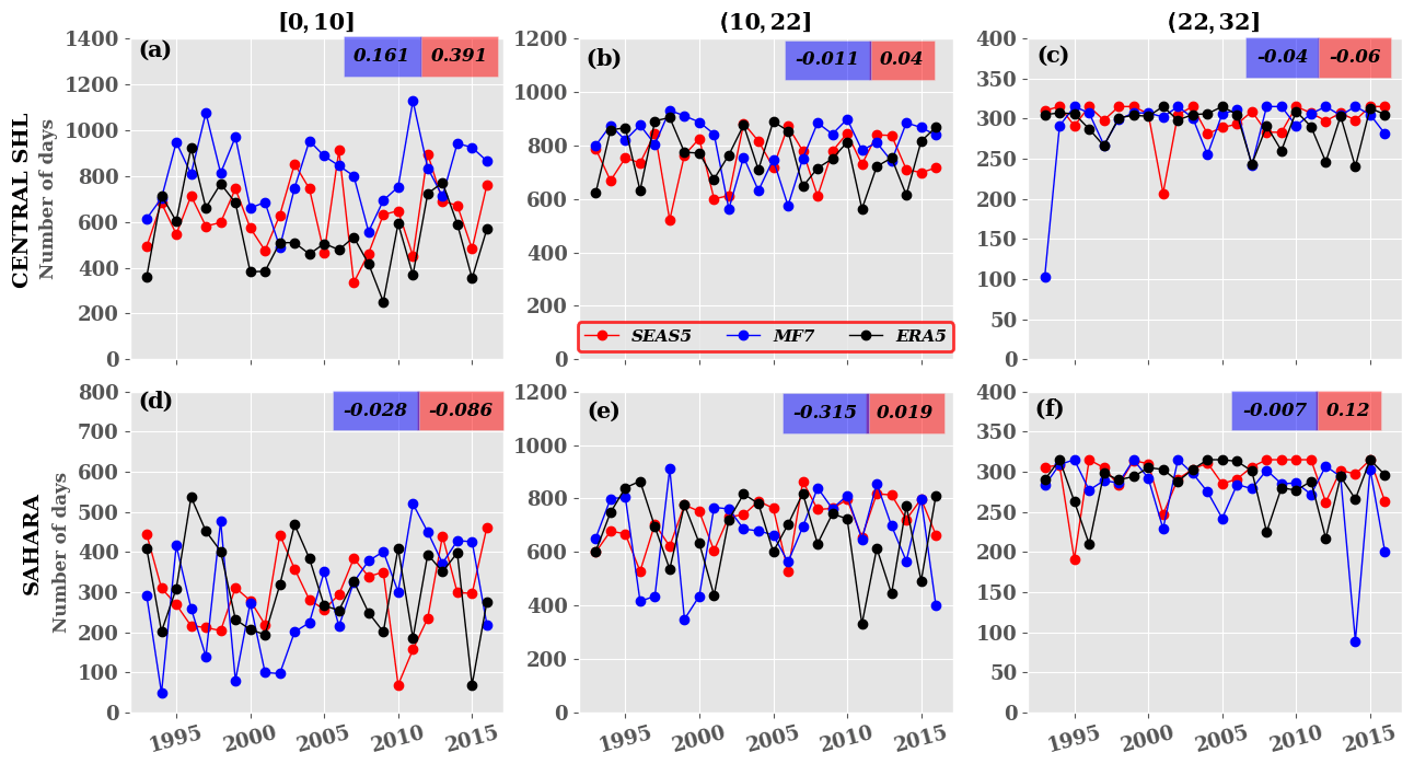
Figure 4 Interannual variability of significant days: significant days here refer to days with a spectral power signal greater than 1. Red, blue and black curves represent the number of days for SEAS5, MF7, ERA5 respectively over the (a–c) central SHL and (d–f) Sahara. The values in red and blue boxes refer to the correlation between SEAS5 and ERA5 and between MF7 and ERA5 respectively. The terms [0,10], (10,22] and (22,32] are the different classes of days identified for the present study. The computation was made just using the unperturbed member of the ensemble forecast models launched from 1 June for the JJAS period. The y axis represents significant days and x axis the year.

3.3 Seasonal cycle

In this section, we are assessing the spatial representation of the SHL over the Sahara region. In order to do that, we evaluate the bias between the seasonal forecast models (SEAS5, MF7) and ERA5 (Fig. 5). The bias is defined here as the difference between the forecasts and the reanalyses; the mathematical expression of the bias is the following:

$$\begin{array}{}\text{(9)}& {\displaystyle }{B}_t=F_t-R_t,\end{array}$$

where F_t and R_t are the forecasts and reanalyses respectively at time t.

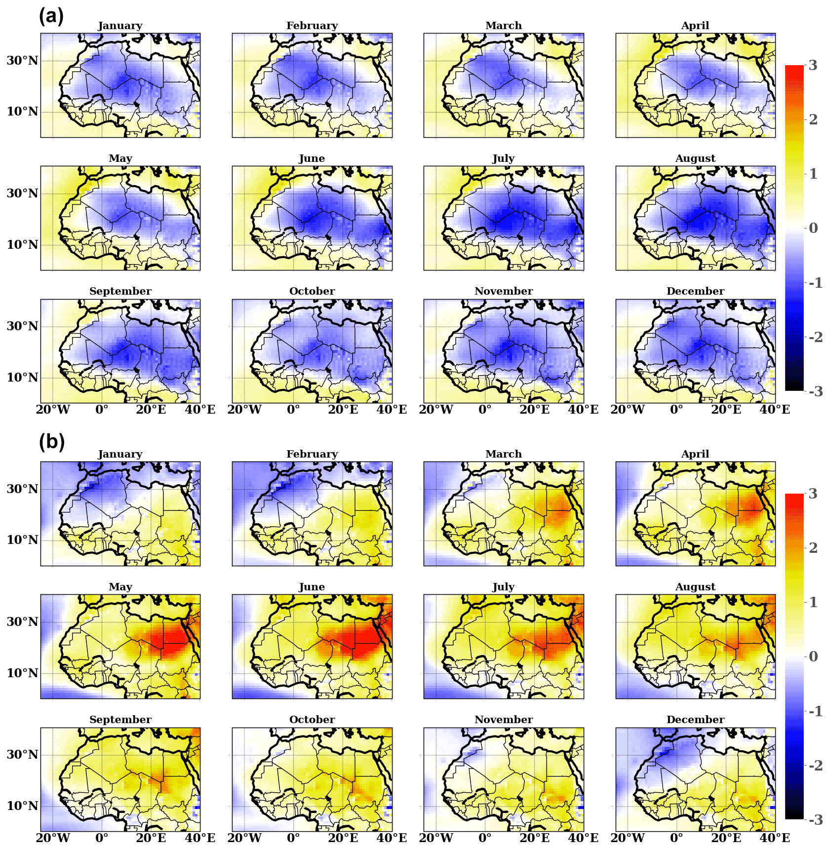
Figure 5 Climatology of monthly bias temperature over the Sahara region during 1993–2016 between (a) SEAS5 and ERA5 and (b) MF7 and ERA5. The bias is computed using daily temperature at 00:00 and 12:00 UTC. The computation was made using the ensemble mean for forecast models. The color bar indicates the bias value in kelvins. The y axis indicates the latitudes and x axis the longitudes of our domain.

The bias is computed for each month at lead time 0 during the season from January to December for the period 1993–2016. By extending the analysis window over the season, we are able to check if the biases in the seasonal forecast models are constant or specific to the JJAS period. When analyzing the SEAS5 model outputs (Fig. 5a), we notice an overestimation of temperature over the Atlantic Ocean and over the Mediterranean Sea. We observe a cold bias between SEAS5 and ERA5 which appears progressively during the first months (January to April) and tends to intensify during the monsoon phase over the Sahel region. This cold bias is centered over the Sahara between the north of Mali, Niger and the south of Algeria and tends to decrease in intensity during the retreat phase of the monsoon in October. SEAS5 is colder than ERA5 and underestimates the spatial evolution of the SHL over the Sahara. In fact, biases in the evolution of the coupled ocean–atmosphere system or in the continental sub-surface can play a role in theses biases, but their investigation is beyond the scope of this paper. The analysis on MF7 shows a progressive appearance of a warm bias in comparison to ERA5 over the Sahel during January and February (Fig. 5b). This warm bias tends to develop from March to September and affects the whole Sahara. It is more intense during the monsoon phase and is located over the eastern part of the Sahara. The bias between MF7 and ERA5 tends to decrease in intensity during the retreat phase of the monsoon in October. MF7 is warmer than ERA5 and overestimates the spatial evolution of the SHL over the Sahara. The central SHL area is less affected by this warming in MF7 compared to the rest of the Sahara. This behavior in the Sahara region, especially in the eastern part of the Sahara, could be related to an underestimation of air advection coming from the Mediterranean regarding the prevalence of the hot bias to the eastern part of the Sahara (Fig. 2b). This analysis shows that the two seasonal forecast models have two contrasted representations of the SHL compared to ERA5, with a colder SHL in SEAS5 and a warmer SHL in MF7, which is in agreement with previous global studies (e.g., Dixon et al., 2017; Johnson et al., 2019). The two seasonal forecast models share however a similar seasonal evolution of the bias (increasing bias during the monsoon season) and a large spatial scale of the bias that covers most of the Sahara. Without sensitivity experiments, it is impossible to clearly identify the reasons for these opposite behaviors between the two models. The investigation of the origins of these biases is well beyond the scope of this article. In a more general framework, various European research projects have shown the difficulty of attributing a specific bias to a specific parameterization over West Africa, including the SHL (Martin et al., 2017).

After the evaluation of the spatial evolution of the SHL in the seasonal forecast models, the representation of the temporal drift is assessed (Fig. 6). The method used here consists in computing the climatology of the daily T850 ensemble mean and ensemble spread for the two models (SEAS5 and MF7) and the daily climatology of T850 for ERA5 from 1993–2016. For the models, we consider only the re-forecasts launched on 1 April, 1 May and 1 June for a period of 6 months (see Sect. 2.4 for more details). We can see that the climatology of ERA5 remains contained in the spread described by SEAS5 for all lead times over the central SHL location and Sahara; this spread in SEAS5 seems to be constant in time and does not increase with the lead time. We observe for the first forecast days a large spread with MF7 which is not present in SEAS5, likely associated with different perturbations and initialization techniques that are beyond the scope of this study. For all lead times, an overestimation of temperature is shown with MF7 over the Sahara around mid-June and later over the central SHL location (∼10 d after 1 July). SEAS5 shows an underestimation of temperature occurring on 1 July over both the central SHL box and the Sahara at different lead times. The maximum intensities of the SHL activity in the two seasonal forecast models are reached during the period of strong activity of the monsoon flux in the Sahel region (July–August). Both models are very consistent at the beginning of the season (April–June) when the Sahara is gradually warming. In the extension of the previous analyses, we decided to check the temporal correlation of the models and ERA5 (Fig. S6). We observe a weak correlation between the evolution of the SHL in the seasonal forecast models and ERA5. The scatterplot analysis used for this evaluation highlights the over/underestimation of T850 in MF7/SEAS5 with respect to ERA5 as observed in the monthly bias analyses (Fig. S6c).

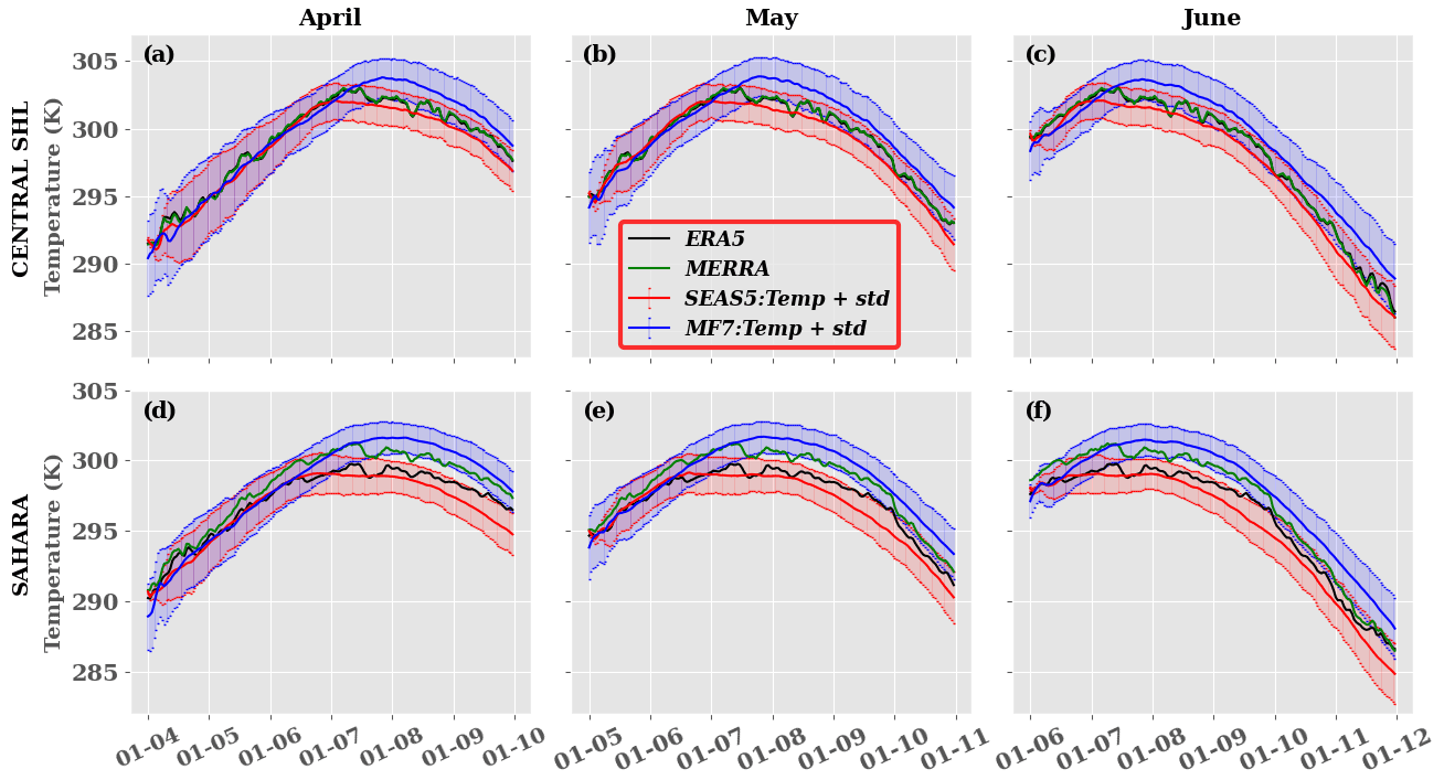
Figure 6 Climatology and spread of mean daily temperature during 1993–2016 at different initialization months for a 6-month forecast: (a, d) April, (b, e) May and (c, f) June for the (a–c) central SHL box and (d–f) Sahara. Bold black, green, red and blue curves refer to the mean T850 of ERA5, MERRA, SEAS5 and MF7 respectively; red and blue bars represent the inter-member spreads for SEAS5 and MF7 respectively. The computation was made using the ensemble mean of forecast models. The y axis indicates temperature in kelvins and x axis the time.

An estimation of bias was carried out for the SEAS5 model data for (i) the full available period, running from 1981 to 2016 (denoted SEAS5₁), and (ii) the period common to MF7 and SEAS5, 1993–2016 (denoted SEAS5₂). The bias evolution is quite similar over the two periods (see Fig. 5a and Fig. S5 in the Supplement); but we notice in SEAS5₁ a smaller cold bias compared to in SEAS5₂. This change in bias intensity can be explained by a warming in SEAS5 re-forecasts during the period 1981–1992 which attenuates the cooling effect in the model during the period 1993–2016.

3.4 Interannual distribution of the T850

The climatological trend of the distribution of SHL intensities has been analyzed using the seasonal probability distribution function (pdf) (Fig. 7a, f) of the SHL box-averaged T850 (used as the proxy for the SHL intensity) over the JJAS period at June lead time 0 (i.e., the initialization of the model was made on 1 June). The analysis of seasonal T850 shows a high variability in ERA5 and the presence of a decadal warming trend from 2005–2016 over both the central SHL location and the Sahara (Fig. 7a, g). The high interannual variability in the SHL seen in ERA5 is underestimated by SEAS5 and MF7. Using raw outputs of the seasonal forecast models, SEAS5 tends to represent much better than MF7 the distribution the SHL intensities over the Sahara (Fig. 7a, c, d and g, i, j). Another specificity of MF7 is its slightly larger ensemble spread. SEAS5 seems to underestimate the warming trends present in ERA5 from 2005–2016, and an overestimation of this trend is observed with MF7 (Fig. S10); this behavior in the seasonal forecast models is present over both the central SHL box and the Sahara. By using this type of visualization (heatmap which is a graphical representation of data where values are depicted by color), it is possible to assess the intensity of the climatological trend with respect to the intraseasonal variability (Fig. 8). The interannual variability in the SHL anomalies distribution in the seasonal forecast models is too far from ERA5, but some characteristics are captured by the models (e.g., the increase in the frequency of anomalies in ERA5 during the 2000s). We observed high frequencies in the SHL anomalies distribution at an interannual timescale for MF7 and SEAS5 with more intense values over the Sahara (Fig. 8b, c, g, h). To focus more on the evolution of the tails of the distribution (i.e., the warmest and coldest T850), the anomaly of the pdf of temperature is provided in supplementary materials (Fig. S7). An increase in the occurrence of the warmest temperature is observed in SEAS5 and MF7 during the 2010s. MF7 tends to overestimate the interannual variability in the coldest and warmest temperature distribution, and SEAS5 exhibits an overall trend with some features close to ERA5. Despite the fact that seasonal models tend to capture some characteristics of the SHL variability, large differences are observed in comparison with ERA5. These differences can be explained by systematic biases present in models, as well as by approximations made during the models implementation (initial and boundary conditions, physical hypotheses, etc.). In order to improve the quality of the forecast, bias correction methods have been applied.

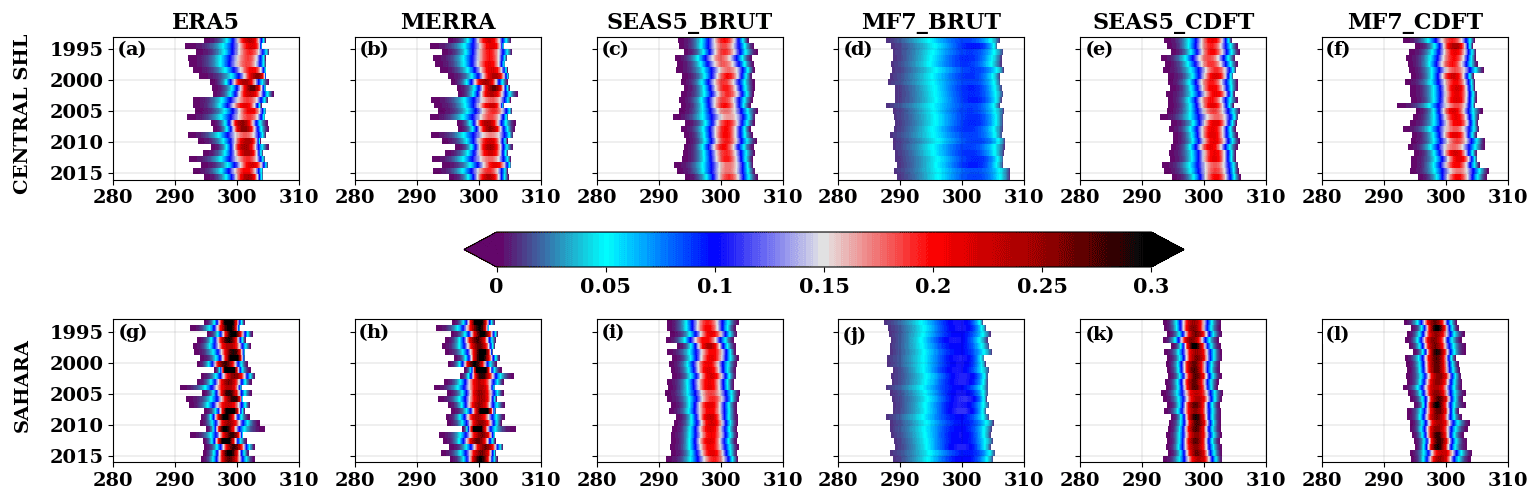
Figure 7 Distribution of yearly T850 over the JJAS period during 1993-2016 over the (a–f) central SHL box and (g–l) Sahara. ERA5, MERRA, SEAS5_BRUT and MF7_BRUT here correspond to the intensity of the SHL using ERA5 and MERRA for the reanalyses; SEAS5 and MF7 raw forecasts respectively. SEAS5_CDFT and MF7_CDFT refer to the intensity of the SHL using SEAS5 and MF7 seasonal forecasts respectively bias corrected using ERA5. The computation was made using the ensemble members of the forecast models. The y axis indicates time in years and x axis T850 in kelvins. The color bar indicates the probability of occurrence.

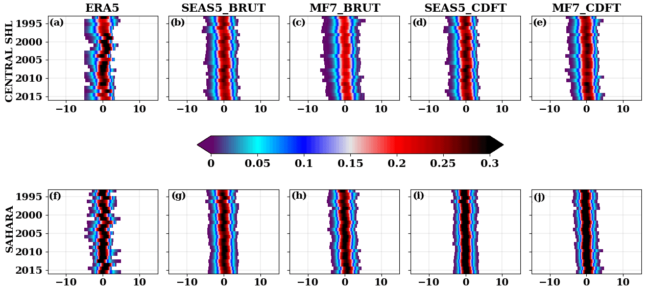
Figure 8 Same as Fig. 7 but for the yearly anomalies of temperature. The anomalies are computed by removing the daily climatology temperature for each year.

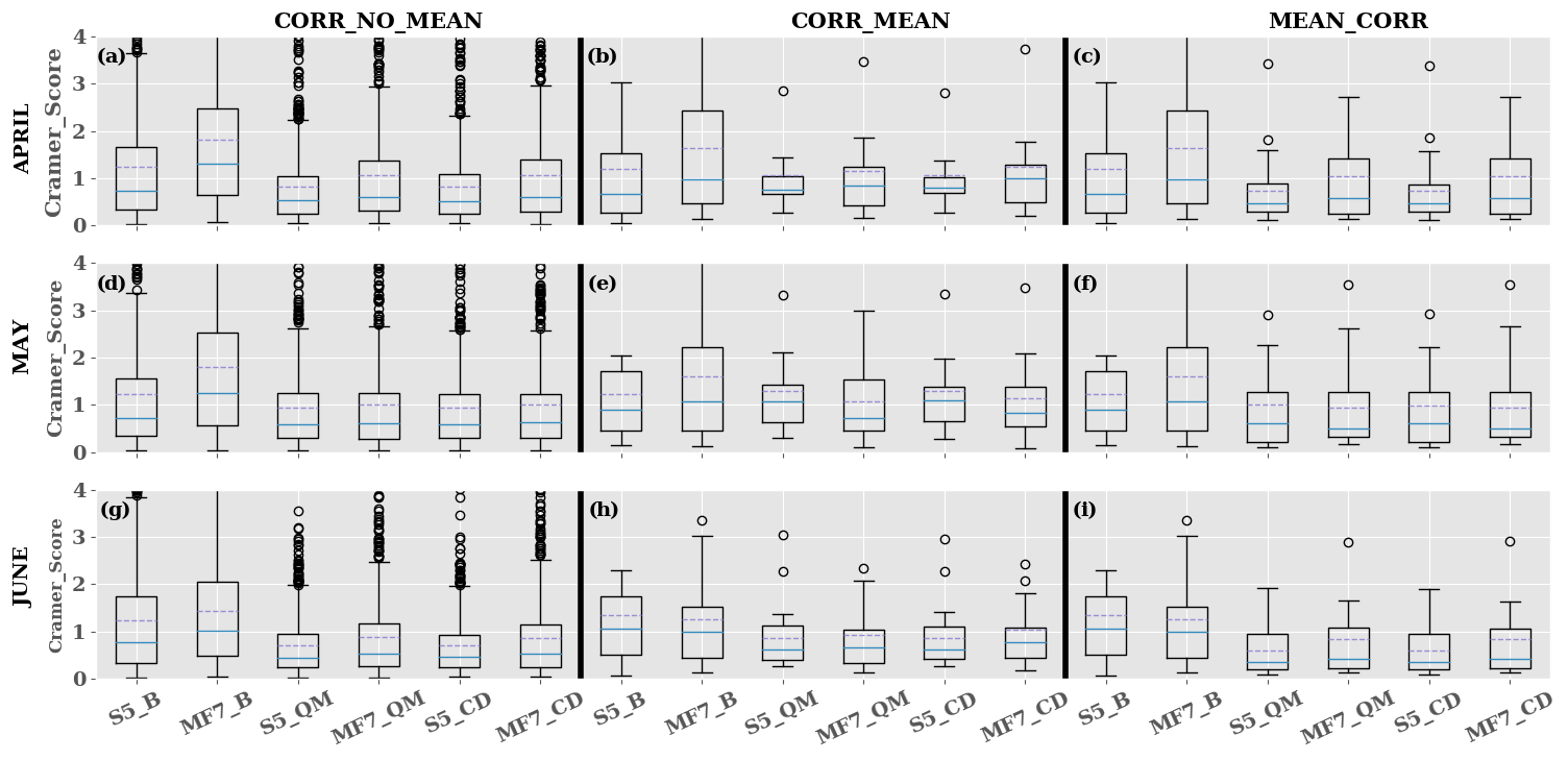
Figure 9 Bias correction evaluation using Cramér–von Mises score over the JJAS period during 1993–2016 on the central SHL box at different forecast initialization months: (a–c) April, (d–f) May and (g–i) June. The CORR_NO_MEAN, CORR_MEAN and MEAN_CORR methods are well described in Sect. 3.4. S5_B, S5_CD and S5_QM represent the Cramér score computed using the SEAS5 raw forecasts, SEAS5 corrected with CDF-t and QMAP methods respectively. The same applies to MF7_B, MF7_CD and MF7_QM with the MF7 model. The y axis indicates the Cramér score and x axis the different products used for the computation of the Cramér score.

The above analyses revealed the presence of biases in the models; bias correction was applied over the JJAS period for June lead times 2, 1 and 0 (which represent the forecast of the JJAS period initialized in April, May and June respectively). The bias correction techniques used are CDF-t and QMAP (see Sect. 2.5.2 for more details on their application). The analysis of ensemble forecast models remains very delicate because of the many possible ways to approach the bias correction; i.e., should we use the unperturbed member, mean ensemble member, median ensemble member or the whole ensemble member? In our case, the bias correction is first applied separately to the ensemble members in order to correct the re-forecasts of each of the 25 members of the seasonal forecast models (SEAS5 and MF7). A second methodology has been tested by applying a bias correction to the ensemble mean. To evaluate the sensitivity of the Cramér score to the ensemble forecast models, we defined three different approaches as follows:

• CORR_NO_MEAN. In this approach the bias correction is applied to the whole ensemble member and the Cramér score is computed using the outputs of the correction.

• CORR_MEAN. Here we compute first the mean over the outputs of the bias correction on the whole ensemble member; and we use this mean to compute the Cramér score;

• MEAN_CORR. The method consists of applying the bias correction to the ensemble mean, and the computation of the Cramér is performed directly using the outputs of the correction.

The Cramér score was calculated firstly using ERA5 and the raw forecast samples (SEAS5 and MF7) and secondly between ERA5 and the bias-corrected forecast samples (Fig. 9). We can observe that raw forecasts are not improved with initialization months (April, May or June) while corrected forecasts show an improvement with decreasing lead times. This can be the result of systematic bias in seasonal forecast models. The MEAN_CORR method (Fig. 9c, f, i) is more efficient than the two other approaches CORR_MEAN and CORR_NO_MEAN, based on the Cramér score values. The CORR_MEAN approach tends to smooth the corrected forecasts due to the computation of the mean ensemble member after applying the correction. CDF-t and QMAP methods produce very similar results; an illustration of the corrected forecasts using both the methods is provided in supplementary materials (see Fig. S9). MF7 raw forecasts show relatively large correction over the Sahara (Fig. S8); this behavior in MF7 is related to the hot bias occurring over the eastern part of Sahara during the JJAS period as mentioned in Sect. 3.2 (Fig. 5b). We can see from these results that bias corrections are efficient and so important to apply to the model outputs. Some illustrations of the corrected forecasts have been made with the CDF-t method. In Fig. 7e and j, we can notice a significant improvement in the distribution of SHL in MF7 over both the central SHL location and the Sahara. This improvement is also effective for SEAS5 (Fig. 7d, i). The corrected forecast distributions are closer to ERA5 than the raw forecast ones. The investigation of the correlation between the corrected forecasts and ERA5 (Fig. S6b, d) shows clearly that CDF-t corrects the cold/hot bias in SEAS5/MF7 by increasing/decreasing T850 values in order to match with ERA5 T850 values. CDF-t reduces a large part of the biases in SEAS5 and MF7, but the interannual correlation with ERA5 is not improved. Indeed, CDF-t is a quantile-based univariate bias adjustment method. As such, it preserves the ranks of the model simulations and thus preserves their rank (Spearman) correlations as well (e.g., Vrac, 2018; François et al., 2020).

3.5 Evolution of the extreme SHL events

Strong SHL activity contributes to the reinforcement of the monsoon flow over the Sahel along the eastern flank of the SHL. It also modulates the intensity of the AEJ and generates wind shear over the region. The resulting wind shear will generate more instabilities favoring convective activities over the West Africa region. Taylor et al. (2017) showed that strong SHL activity intensifies the convection within the meso-scale convective systems (MCSs). Fitzpatrick et al. (2020) suggest that stronger wind shear may be a key driver of decadal changes in storm intensity in the Sahel. This shows the importance of having a good representation of these SHL characteristics in the models. Therefore, we analyzed the variability in the SHL extremes using the raw and corrected forecasts obtained with CDF-t (Fig. 10). We distinguished cold and hot extremes which represent events under the quantile 10 % and above the quantile 90 % respectively. We observe an increase in the SHL hot extremes in the seasonal forecast models during the 2010s as well as a diminution of the SHL cold extremes which is in agreement with the evolution in ERA5. MF7 raw forecasts tend to overestimate the SHL hot extremes, while they seem to underestimate the SHL cold extremes over both the central SHL location and the Sahara. SEAS5 raw forecasts underestimate the SHL hot extremes and make an overestimation of the SHL cold extremes over the Sahara. We can see the efficiency of the bias correction (CDF-t) when analyzing the evolution of the SHL extremes from the corrected forecasts. Despite the difference between ERA5 and the corrected forecasts being reduced compared to the raw forecasts, the observed gap remains significant.

Figure 10 Interannual variability in the SHL extremes over the (a, b) central SHL and (c, d) Sahara during the JJAS period from 1993 to 2016. SEAS5_C and MF7_C refer to corrected forecasts with the CDF-t method, and SEAS5_B and MF7_B represent raw model forecasts. The x axis indicates the time (year) and y axis the number of extremes registered for each year. Hot extremes are events occurring above the 90th percentile, and cold extremes are associated with events below the 10th percentile.

3.6 East–west pulsation modes

The SHL has a typical timescale of 15 d associated with low-level horizontal advection of moist and cold air that modulates the surface temperature on the eastern part of the Sahara and makes the maximum surface temperature shift from a more eastern to a more western location of the Sahara (Chou et al., 2001; Roehrig et al., 2011), leading to so-called heat low east (HLE) events and heat low west (HLW) events respectively (Chauvin et al., 2010). Roehrig et al. (2011) and Lavaysse et al. (2011) highlighted interactions between SHL components and Sahelian rainfall events. In the present work, a simple method is proposed to capture the HLW and HLE oscillations. Our method consists in defining a dipole by computing the mean T850 difference between HLW and HLE boxes, here referred to as WSHL and ESHL respectively (see Sect. 2.2 for more details):

$$\begin{array}{}\text{(10)}& Dipole=HLW-HLE\end{array}$$

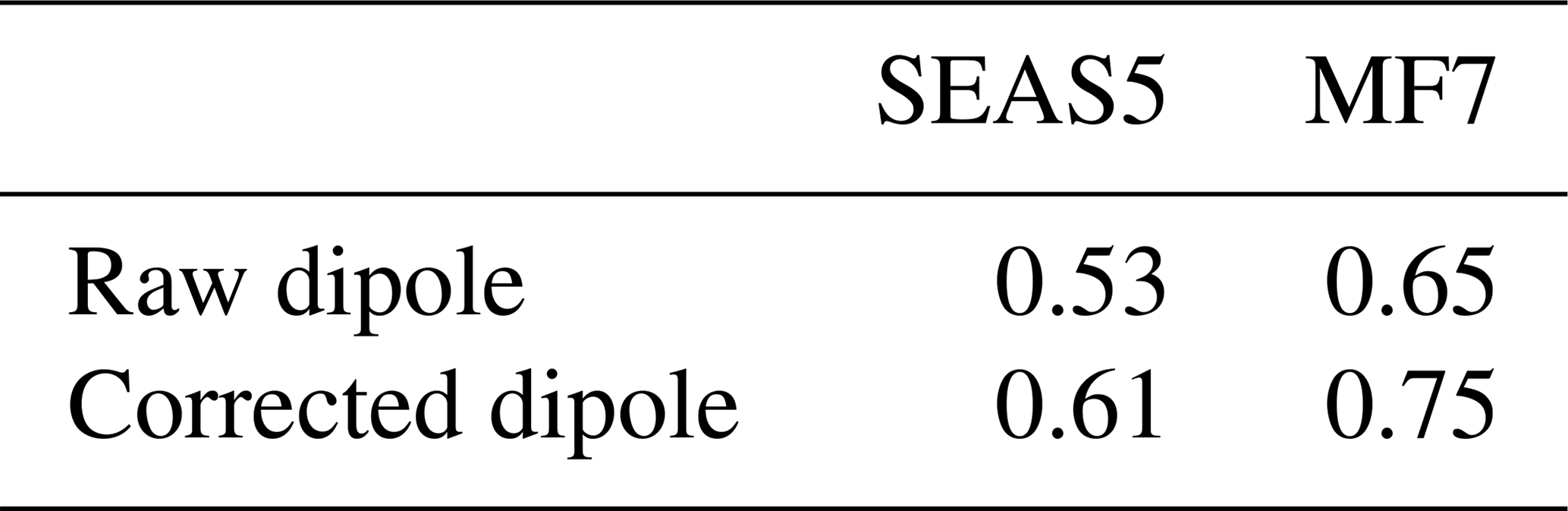
A positive value of the dipole indicates an HLW occurrence, while a negative value corresponds to the HLE event. We evaluate the method using the LLAT approach and the automatic detection of the SHL barycenter (Lavaysse et al., 2009) used during the H2020 Dynamics–Aerosol–Chemistry–Cloud Interactions in West Africa (DACCIWA) project campaign (Knippertz et al., 2017), which aims to evaluate the seasonal location of the SHL with respect to its climatological position. An illustration of our method for the year 2005 is shown in Fig. S11 and confirms that there is a good agreement between the evolution of the dipole of T850 in ERA5 and the SHL barycenter computed in Knippertz et al. (2017). After the assessment of the detection method, we evaluate the representation of the SHL components in the seasonal forecasts and ERA5 data (Fig. 11a). As the corrected forecasts are unbiased compared to the raw forecasts, we use them for this analysis. The results show that ERA5 presents a bimodal regime; the first one is less accentuated and associated with the HLE events (negative dipole value), while the second regime is more representative and related to HLW events (positive dipole value). For MF7, we also noticed a bimodal regime and a large range in the distribution of the dipole compared to ERA5; the first regime is more frequent and associated with the HLE events. The second regime is less frequent and related to HLW events. With SEAS5, we also observed a bimodal regime and a reduced range compared to ERA5. The first regime is less important and associated with the HLE events, while the second one is more important and related to HLW events. From this analysis, we can notice that MF7 (SEAS5) tends to overestimate the HLE (HLW) phases (Fig. 11a). This behavior in the seasonal models is well highlighted when using the raw forecasts for the computation of the dipole (see Fig. S16a in the Supplement). MF7 and SEAS5 here again exhibit opposite behaviors in terms of frequencies and intensities of the SHL components. The analysis of the correlation between the models and ERA5 shows that MF7 seems to be slightly better correlated with ERA5 than SEAS5 (see Table 1). We noticed a little and not significant improvement in the correlation with the corrected signal.

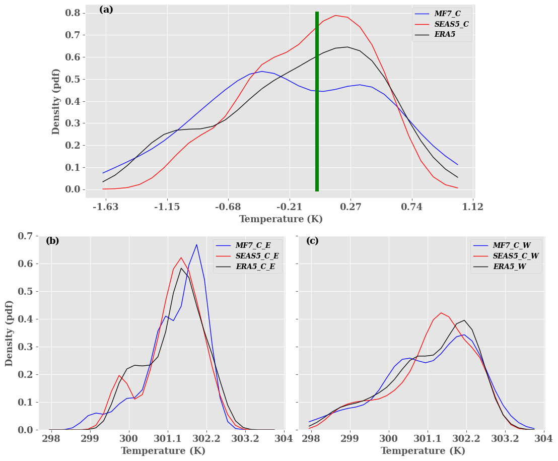
Figure 11 Distribution of the climatology over the period 20 June–17 September from 1993 to 2016 at June lead time 0 for (a) the dipole which represents the difference between heat low west and heat low east, (b) heat low east, and (c) heat low west. MF7_C and SEAS5_C refer to the MF7 and SEAS5 forecasts respectively corrected with the CDF-t method. ERA5_E, MF7_C_E and SEAS5_C_E refer to the HLE in the reanalyses and MF7 SEAS5 forecasts respectively corrected with the CDF-t method. “ERA5_W”, “MF7_C_W” and “SEAS5_C_W” refer to the HLW in the reanalyses and MF7 and SEAS5 forecasts respectively corrected with CDF-t method. The y axis indicates the probability of occurrence and x axis the temperature in kelvins. The vertical green bar represents the boundary between the HLE and HLW phases. The analysis was carried out using the unperturbed member.

Table 1 Correlation between the dipole values derived from the seasonal models (SEAS5 and MF7) and the one derived from ERA5. The “Raw dipole” represents the dipole computed using raw forecasts and “Corrected dipole” that using the bias-corrected forecasts.

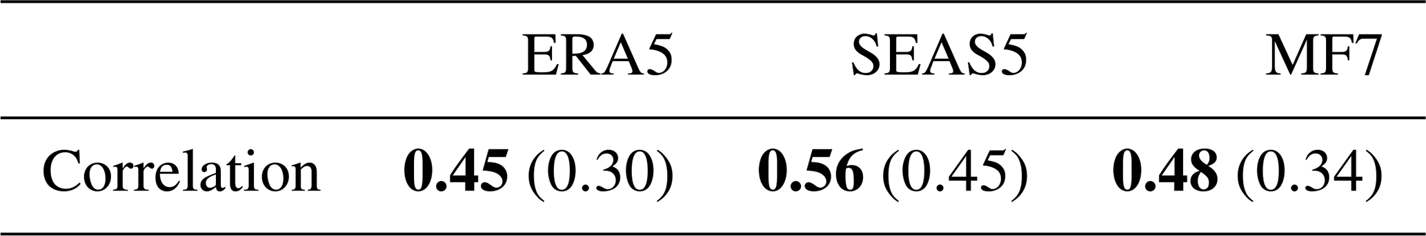
To better understand the reasons for these differences, a separate analysis of the SHL distribution in the two boxes is performed (Fig. 11b, c). First, it is worth noting that the east Sahara is climatologically hotter than the west Sahara in ERA5, SEAS5 and MF7. This is explained by the proximity of the west Sahara to the Atlantic Ocean and the advection of fresh air masses in that area (see Fig. 2 for the location of the west Sahara). Hence, there is a greater occurrence of the HLE events compared to the HLW phases in ERA5. The models (SEAS5/MF7) are able to reproduce this partitioning of the SHL phases observed in ERA5 with the same range of frequencies ($\sim \mathrm{0.6}/\mathrm{0.4}$) for HLE/HLW respectively. Both models overestimate the occurrence of the HLE events; MF7 tends to develop hot HLE events (Fig. 11b). The analysis of the HLW phases reveals an under/overestimation of the intensity/occurrence of these events in SEAS5. We notice, with MF7, a good representation of the intensity of the HLW events with sometimes an overestimation of the frequencies associated with these phases (Fig. 11c). The interactions between the east and west boxes are investigated through a correlation analysis using the outputs of both the seasonal models. The results obtained using raw and corrected forecasts are very similar (not shown), so in the following we present only the results related to the bias-corrected forecasts. High correlation would suggest an influence of the large-scale processes, whereas low correlation would indicate that smaller-scale processes and local impacts come into play. The correlation between HLE and HLW phases is about 0.45, 0.56 and 0.48 for ERA5, SEAS5 and MF7 respectively (see Table 2). SEAS5 shows a higher correlation between the two phases compared to ERA5 and MF7. To discriminate the effect of the intraseasonal and seasonal cycles, the correlations are computed between HLW and HLE by using the daily T850 anomalies relative to the daily climatology of T850 in the two boxes. As expected, the seasonal cycle has a strong impact and the correlation reduces from 0.45 to 0.30 for ERA5 compared to a reduction from 0.56 to 0.45 for SEAS5 and from 0.48 to 0.34 for MF7 (see Table 2). The correlation with SEAS5 remains high compared to MF7 and ERA5; this suggests that T850 over the Sahara in SEAS5 is more affected by large-scale drivers that provide wider temperature field anomalies. MF7 shows a partitioning of SHL variability between the SHL intraseasonal mode and the seasonal cycle that is more in agreement with ERA5. An investigation of the representation of the SHL phases in the models vs. ERA5 has been assessed using the corrected forecasts. The models are more correlated with ERA5 for the HLW phases (see Table S1). Despite the differences between seasonal models and ERA5, the models are able to capture the seasonal east–west migration of the SHL.

Table 2 Correlation between the HLW and HLE phases: values in bold (parentheses) indicate the correlation using the bias-corrected temperatures (anomalies of temperature) over the east and west SHL boxes.

4 Discussion

Our results show that the two seasonal forecast models have the capability to capture some of the SHL main characteristics. There is a deficit in reproducing the intensity and the occurrence of events, such as east and west phases of the SHL, as they appear in the reference ERA5. The analysis of the bias in seasonal forecast models evidenced a hot bias in MF7 and a cold bias in SEAS5 which could be explained by large-scale processes and forcings occurring at different timescales in the Sahara region. The different behaviors observed in forecast models can be related to their sensitivity to the drivers and the physical processes involved in the SHL evolution.

Figure 12 Evaluation of the interannual variability in the SHL over the JJAS period and separately in June, July, August and September during 1993–2016 using monthly mean T850 over the central SHL box at different initialization months: (a–e) April, (f–j) May and (k–o) June. S5_B and S5_C represent respectively the CRPS evaluated using the SEAS5 raw and corrected forecast respectively with the CDF-t method. The same applies for MF7_B and MF7_C with the MF7 model. MS_C represents the CRPS evaluated on the multi-model formed by SEAS5 and MF7 corrected forecasts with the CDF-t method. The computation was made using the ensemble member for both corrected and raw forecasts. The y axis indicates the CRPS values and x axis the data type used for the computation of the CRPS.

A preliminary assessment of the quality of the forecasts with respect to the ERA5 reanalysis is discussed. This is performed through an evaluation of the skills of the seasonal forecast models to reproduce the interannual variability in the SHL. For this evaluation, we used two metrics: the CRPS and RMSE (see Sect. 2.5.3 for more details). A first analysis of the forecasts at an interannual timescale was conducted using monthly mean T850 and daily T850 respectively for the computation of the CRPS (Figs. 12 and S12) and the RMSE (Fig. S14) with initialization of the seasonal forecast models in April, May and June. The first period of evaluation is the seasonal timescale that provides a benchmark of the forecast for the rainy season (Fig. 12a, f, k; see also Fig. S14a, f, k in the Supplement). It gives a limited but significant improvement with respect to the climatology. The scores (CRPS, RMSE) are then decomposed by month (Fig. 12b–e, g–j, l–o) (see also Fig. S14a–e, g–j and l–o in the Supplement) to investigate the representation of the intraseasonal variability in the SHL. We noticed an increase in the CRPS and RMSE values with the lead times over the CSHL location, which leads to a loss of predictability in the seasonal forecast models. SEAS5 shows more predictive skills over the CSHL location for short-lead-time forecasting (0 to 1 months), and MF7 is a little better for long lead times (approximately 3 months). MF7 raw forecasts show very limited skills over the Sahara (see Figs. S12 and S13b in the Supplement); this behavior in MF7 can be related to hot biases evidenced in Sect. 3.2 (Fig. 5a). Bias correction improves considerably the predictive skills of the models. The effect of bias correction on the predictive skills of the seasonal models is more efficient over the Sahara (see Figs. S12 and S13b in the Supplement). This can be explained by the fact that climate models usually take into account large-scale variability. As the Sahara is larger than the central SHL box, the forecast models will better represent the variability occurring over the Sahara; and the correction method will adjust the systematic bias present in the models. Models present lower predictive skills for the daily T850, and an improvement is seen at a monthly timescale for short lead times. However, the correlation found at a monthly timescale never exceeds 0.61 (see Fig. S15b in the Supplement); at a daily timescale, the correlation is less than 0.53 (see Fig. S15a in the Supplement) for all months at lead time 0. Correlations at different lead times have also been computed, but the resulting coefficients were even lower than those obtained at lead time 0 (not shown). An evaluation of the seasonal forecast models at a very short lead time has been performed for June, July, August and September at lead time 0 by computing the CRPS using daily T850 raw forecasts (see Fig. S14 in the Supplement); similar results have been found with the unbiased forecasts (not shown). We observed a progressive increase in the CRPS with time before reaching the predictability horizon at around 20 d. SEAS5 shows predictive skills at the first time steps of 1–3 d over the CSHL and 1–8 d over the Sahara location; and MF7 is more affect by the spin-up at the beginning of the prediction. This behavior in SEAS5 can be explained by the capacity of the model to represent large-scale variability occurring at the Sahara location. From these results, we observed some predictive skills in the seasonal forecast models at an intraseasonal timescale; however they remain weak for a long period and for lead times beyond 1 month. These results are in agreement with previous works which addressed the predictive skills of the ECMWF ensemble system (Haiden et al., 2015).

As seen previously, MF7 and SEAS5 present different characteristics in terms of bias, particularly regarding HLW and HLE event detection. This suggests that a multi-model ensemble approach may be a solution to improve the forecast skills of the seasonal models. Surprisingly, the multi-model shows a predictive skill comparable to the individual models (Fig. 12). This shows that the predictive skills of an ensemble model do not depend on the number of members in the models.

5 Conclusions

This work assessed the representation of the SHL in two seasonal forecast models (SEAS5 and MF7) using ERA5 reanalyses as reference. The choice of ERA5 as reference for this evaluation was supported by a sensitive study conducted between ERA5 and another reanalysis dataset, namely MERRA. Very high correlations have been found between the two reanalyses data, i.e., around 0.97 and 0.92 over the CSHL and the Sahara location respectively; robust similarities are also observed in the yearly distribution of T850. The discrepancies between the reanalyses are much smaller than the biases in the seasonal forecast models with respect to ERA5. Through a set of analyses, we have found opposite biases in the seasonal forecast models compared to ERA5. MF7 has a warm bias and tends to overestimate the intensity of the SHL with respect to ERA5. SEAS5 develops a cold bias and tends to underestimate the intensity of the SHL over the Sahara. The models are able to represent the mean seasonal cycle of the SHL and capture some characteristics of its interannual variability like the warming trends observed during the 2010s. However, the good representation of this interannual variability remains challenging for the models. SEAS5 represents more realistically the climatic trend of the SHL than MF7. The bias correction methods CDF-t and QMAP are very efficient at reducing the systematic bias present in the seasonal models. By using bias correction tools, the results highlight the capacity of the models to represent the intraseasonal pulsations (the so-called east–west phases) of the SHL. We notice an overestimation of the occurrence of the HLE phases in the models (SEAS5 and MF7); the HLW phases are much better represented in MF7. This diagnosis is a first validation of the representation of the SHL in seasonal models. In spite of this, the correct timing of these pulsations is still a key challenge and the next step forward. Seasonal forecast models show predictive skills at an intraseasonal timescale for short periods. Bias correction contributes to improving the ensemble forecast score (CRPS), but the forecast skill remains weak for a lead time beyond 1 month. The issue of the lack of correlation in models cannot be solved through a bias correction approach; only model improvements could provide better correlations between forecasts and observations. In a future study, we will investigate the relationship between the SHL and the extreme rainfall in the Sahel region at an intraseasonal timescale.