the Creative Commons Attribution 4.0 License.
the Creative Commons Attribution 4.0 License.
 | 06 Oct 2021
Occurrence and transition probabilities of omega and high-over-low blocking in the Euro-Atlantic region
Annette Müller
Lisa Schielicke
Peter Névir
Henning W. Rust
Stationary, long-lasting blocked weather patterns can lead to extreme conditions such as anomalously high temperatures or heavy rainfall. The exact locations of such extremes depend on the location of the vortices that form the block. There are two main types of blocking: (i) a high-over-low block with a high located poleward of an isolated low and (ii) an omega block with two lows that lie southeast and southwest of the blocking high in the Northern Hemisphere. In this work, we refine a novel method based on the kinematic vorticity number and the point vortex theory that allows us to distinguish between these two blocking types. Based on the National Centers for Environmental Prediction–Department of Energy (NCEP–DOE) Reanalysis 2 data, we study the trends of the occurrence probability and the onset (formation), decay (offset) and transition probabilities of high-over-low and omega blocking in the 30-year period from 1990 to 2019 in the Northern Hemisphere (90∘ W–90∘ E) and in the Euro-Atlantic sector (40∘ W–30∘ E). First, we use logistic regression to investigate long-term changes in blocking probabilities for full years, seasons and months. While trends are small for annual values, changes in occurrence probability are more visible and also more diverse when broken down to seasonal and monthly resolution, showing a prominent increase in February and March and a decrease in December. A three-state multinomial regression describing the occurrence of omega and high-over-low blocking reveals different trends for both types. Particularly the February and December changes are dominated by the omega blocking type. Additionally, we use Markov models to describe transition probabilities for a two-state (unblocked, blocked) and a three-state (unblocked, omega block, high-over-low block) Markov model. We find the largest changes in transition probabilities in the summer season, where the transition probabilities towards omega blocks significantly increase, while the unblocked state becomes less probable. Prominent in winter are decreasing probabilities for transitions from omega to high-over-low and persistence of the latter. Moreover, we show that omega blocking is more likely to occur and to be more persistent than the high-over-low blocking pattern.
- Article
(8712 KB) - Full-text XML
-
Supplement
(24267 KB) - BibTeX
- EndNote


A blocking is a quasi-stationary, persistent large-scale atmospheric flow pattern that blocks the typical westerly flow and forces the jet and embedded pressure systems to bypass on its northern and southern sides (e.g., Rex, 1950). Blocks can last for several days up to weeks. Typically, a minimum blocking duration of 4 to 10 d is assumed (e.g., Rex, 1950; Pelly and Hoskins, 2003; Barriopedro et al., 2006, 2010; Barnes et al., 2011). Northern Hemisphere blocks are characterized by a steady high-pressure area accompanied by one low-pressure area southwards, called high-over-low, or by two low-pressure systems southwest- and southeastwards of the high, called omega block (see e.g., Bott, 2012; Woollings et al., 2018). Transitions between the different blocking types can be observed: an example is documented in Schielicke (2017, Appendix A3, Fig. A69) for summer 2010, where long-lasting blocking caused extreme heat and forest fires over Russia, while downstream of the blocks “record-breaking” floods occurred in Pakistan (Hong et al., 2011; Schneidereit et al., 2012). Due to their persistence and quasi-stationarity, blocks can determine the weather, especially temperature and precipitation patterns, in a large region over a long period of time. Depending on their location, duration and intensity, these weather situations can have devastating, regional impacts ranging from heat waves and droughts in the warm season to cold spells in winter and spring (e.g., Pfahl and Wernli, 2012; Russo et al., 2015; Brunner et al., 2017, 2018; Hari et al., 2020). Furthermore, the blocking type, i.e., high-over-low or omega block, determines the location of observed or expected extreme weather phenomena. For example, in June and July 2019, omega blocking caused record-breaking temperatures far above 40 ∘C at several locations in western and central Europe (Vautard et al., 2020), with an observed record temperature of 45.9 ∘C in southern France (Henley et al., 2019) and 41.2 ∘C in western Germany (Deutscher Wetterdienst, 2020, 2019; Bissolli et al., 2019). In May and June 2018, an unusually high number of slow-moving thunderstorms caused heavy rain rates and flash floods in large parts of western and central Europe located at the western flank of a quasi-stationary blocking over northern Europe (Mohr et al., 2020). Hence, we expect that the knowledge of the blocking type can help to better estimate the regions which will be impacted.
In order to classify blocking types, the point vortex model can be used. This idealized model gives one conceptual explanation of the quasi-stationarity of atmospheric blocking (see e.g., Obukhov et al., 1984; Kuhlbrodt and Névir, 2000; Müller and Névir, 2014; Müller et al., 2015). It represents a Lagrangian formulation of the vorticity equation with vortices pictured as “particles” with circulation being conserved for each vortex1. The motion of a set of point vortices is determined by their circulations and the intervortical distances only; see e.g., Aref (1979) and Newton (2001). Hirt et al. (2018) statistically confirmed the theory of Müller et al. (2015) that the omega blocking pattern can be regarded as a three-point vortex system (or tripole). If these three vortices form an equilateral triangle (i.e., arranged as in Fig. 1b) with the sum of their circulations being zero, the point vortex system moves westwards opposing the typical westerly flow of the mid-latitudes. Stationarity is achieved when the magnitude of the westerly flow matches the translation speed of the point vortex system. Analogously, a high-over-low block can be described by a point vortex pair (or dipole) of zero total circulation that moves westward (see Fig. 1d). The point vortex concept allows us to classify the blocking state into high-over-low or omega as well as to determine the location and intensity of each vortex associated with the block in gridded data. It is now possible to observe transitions between the blocking states within a longer blocking period.
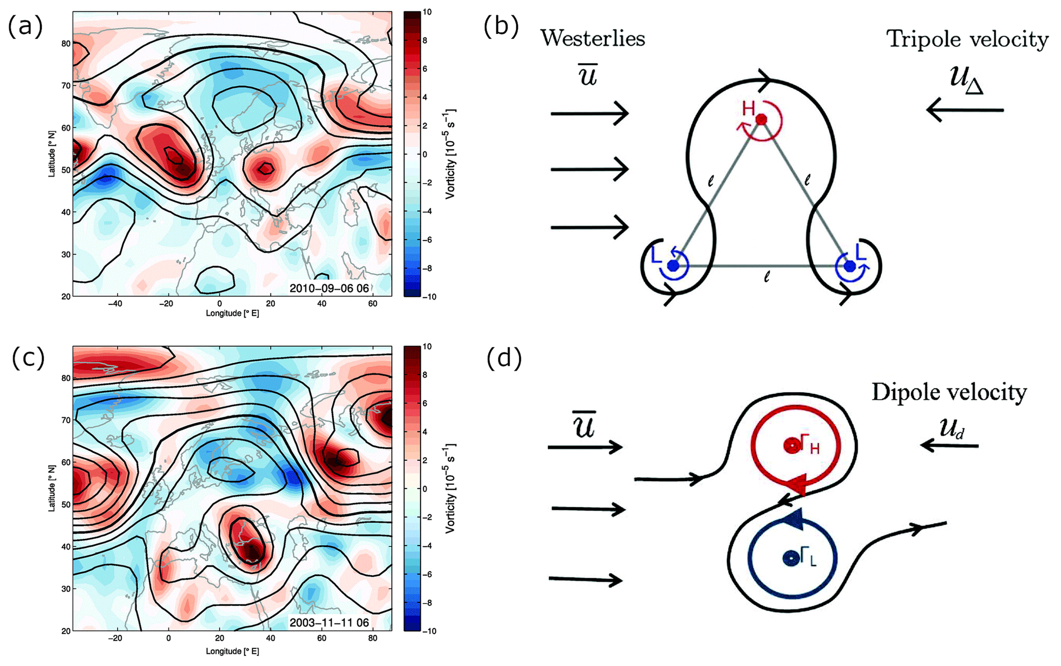
Figure 1Application of point vortex theory to two distinct atmospheric blocking types: (a, b) omega blocking, (c, d) high-over-low blocking. (a, c) Two exemplary blocking events observed at the 500 hPa level: displayed is the relative vorticity (color-shaded) and contours of geopotential height in 8 dm intervals (bold contour represents 552 dm). (b, d) Illustration of how the corresponding blocking can be realized in the point vortex model. Figure is adapted from Hirt et al. (2018, their Fig. 2; published under the terms of the Creative Commons Attribution License (http://creativecommons.org/licenses/by/4.0/, last access: 12 September 2021)) with the upper right figure taken from Müller et al. (2015). The point vortex systems become stationary if the typical westerly flow of the mid-latitudes and the propagation speed of the dipole or tripole point vortex systems are of equal magnitude.
The numerical prediction of blocking onset and persistence, i.e., the transition from zonal to blocked flow and vice versa, is still a challenge. However, it is still important to study these transitions; Ferranti et al. (2015) showed that medium-range ensemble forecasts in the Euro-Atlantic region are less skillful in these situations. One way to describe the probability of transitions between the states of a system is the use of discrete-state Markov models. These models describe the probability of the system in a future state as dependent on the present state only; the future state is hence independent of all previous states (e.g., Grewal et al., 2019). Cluster analyses followed by Markov chains have been used to describe the transitions between different large-scale weather regimes by several authors, e.g., Spekat et al. (1983), Egger (1987), Vautard et al. (1990), and Kimoto and Ghil (1993). Spekat et al. (1983) distinguish between zonal, mixed and meridional weather regimes in central Europe. They found relatively long residence times within the regimes of 5 to 7 d and relatively low daily transition probabilities of 5 % to 11 % between the regimes. However, to the best of our knowledge, the transition between different blocking types within the same blocked period, i.e., the transition from omega to high-over-low and vice versa, has not been studied so far. While blocked periods last for at least 5 d, transitions occur on a smaller timescale, and higher-temporal-resolution data (e.g., 6 h) thus need to be analyzed.
Due to their socio-economic relevance, it is of common interest to study and determine blocking climatologies and trends. It is also observed that the identification of blocking depends on the specific definition and method used (e.g., blocking indices). Blocking climatologies can, furthermore, differ with respect to the frequency and location of blocking (e.g., Barriopedro et al., 2010) and also often depend on the model data (Barnes et al., 2014). Although different methods yield different results, they agree on two general aspects: (i) blocking maxima are observed in the North Pacific and North Atlantic–European region, and (ii) higher blocking numbers occur in boreal winter compared to the summer season, but the details of the climatologies depend on the blocking identification method used (e.g., Fig. 6 in Pinheiro et al., 2019). However, larger variability among methods can be observed even when looking at individual blocking events (Pinheiro et al., 2019) and from year to year (Davini et al., 2012). Davini and D'Andrea (2020) compare the blocking frequency for different regions using different models for the time period 1951–2017. Moreover, analyzing seasonally resolved trends, they find a negative trend in blocking frequency for the Northern Hemisphere in winter and a positive trend in summer. Even though their results show a general decrease in blocking frequency for the future, the impact in some regions and seasons, e.g., the summer Ural blocking, might increase. Barnes et al. (2014) find no general evident increase in blocking over the Northern Hemisphere, but they further show that the results depend on the region, season and also on the analyzed time period. For example, there are significant seasonal increases for some regions, such as Asia in boreal winter and the North Atlantic in boreal summer. Additionally, Cheung et al. (2013) confirm a strong dependence of the blocking frequency on the seasons. Their results indicate that the strength of blocking events, in terms of intensity and extension, is stronger in winter and weaker in summer. But they also state that the impact of summer blocks might be higher. In this work, we study climatologies and annually, seasonally and monthly resolved trends of blocking occurrence probabilities with a novel strategy: blocking type classification based on point vortex theory followed by a description of occurrence and transition probabilities with logistic regression and Markov models. Furthermore, we extend the existing literature on trends in blocking occurrence by the aspect of blocking types. Since these blocking types are connected to different typical regions of high-impact weather, their long-term occurrence trends are of general interest. Hence, we refine the fluid-dynamically based method developed in Hirt et al. (2018) to classify blocking into high-over-low and omega and use logistic regression and Markov models to address the following research questions:
-
Do blocking occurrence probabilities undergo long-term changes? Do these changes depend on season or month?
-
Do onset (formation), decay (offset) or transition probabilities from one blocking type to another undergo long-term changes? Do these changes depend on season or month?
The work is structured as follows. First, we shortly describe the data set and variables in Sect. 2. In Sect. 3.1 to 3.4, we explain the steps of our identification and classification strategy in more detail. Section 3.5 gives a short overview of logistic and multinomial regression for the analysis of occurrence probabilities; Sect. 3.6 introduces discrete-state Markov processes for the analysis of transition probabilities between blocking types. Results follow in Sect. 4 and are discussed subsequently in Sect. 5. We close with a conclusion in Sect. 6.
We use the National Centers for Environmental Prediction–Department of Energy (NCEP–DOE) Reanalysis 2 data set (Kanamitsu et al., 2002) for our analysis. The data have a grid spacing of on a regular latitude–longitude grid and are available every 6 h. In our study, we used a period of 30 years from 1990 to 2019. We restricted the analysis to the 500 hPa level, a level where the divergence of the horizontal wind field is close to zero (Schielicke, 2017). This allows us to apply the principles of point vortex theory, which requires two-dimensional non-divergent flow. We use geopotential height and the horizontal wind components (U,V) at 500 hPa to compare the blocking behavior in two regions. The first region covers half the Northern Hemisphere, from 90∘ W to 90∘ E. The second region is a subset of this larger region, covering the Euro-Atlantic area from 40∘ W to 30∘ E.
In the following we describe the six steps of the analysis, starting from the identification of blocked latitudes (Step 1; Sect. 3.1) and the calculation of blocking properties with the trapezoid method (Step 2; Sect. 3.2) to classification of blocking into omega and high-over-low types (Step 3; Sect, 3.3), followed by the choice of the region of interest (Step 4; Sect. 3.4). Finally, we introduce logistic and multinomial regression to model occurrence probabilities (Step 5; Sect. 3.5) as well as Markov models to describe transition probabilities (Step 6; Sect. 3.6). The steps are summarized in Fig. 2.
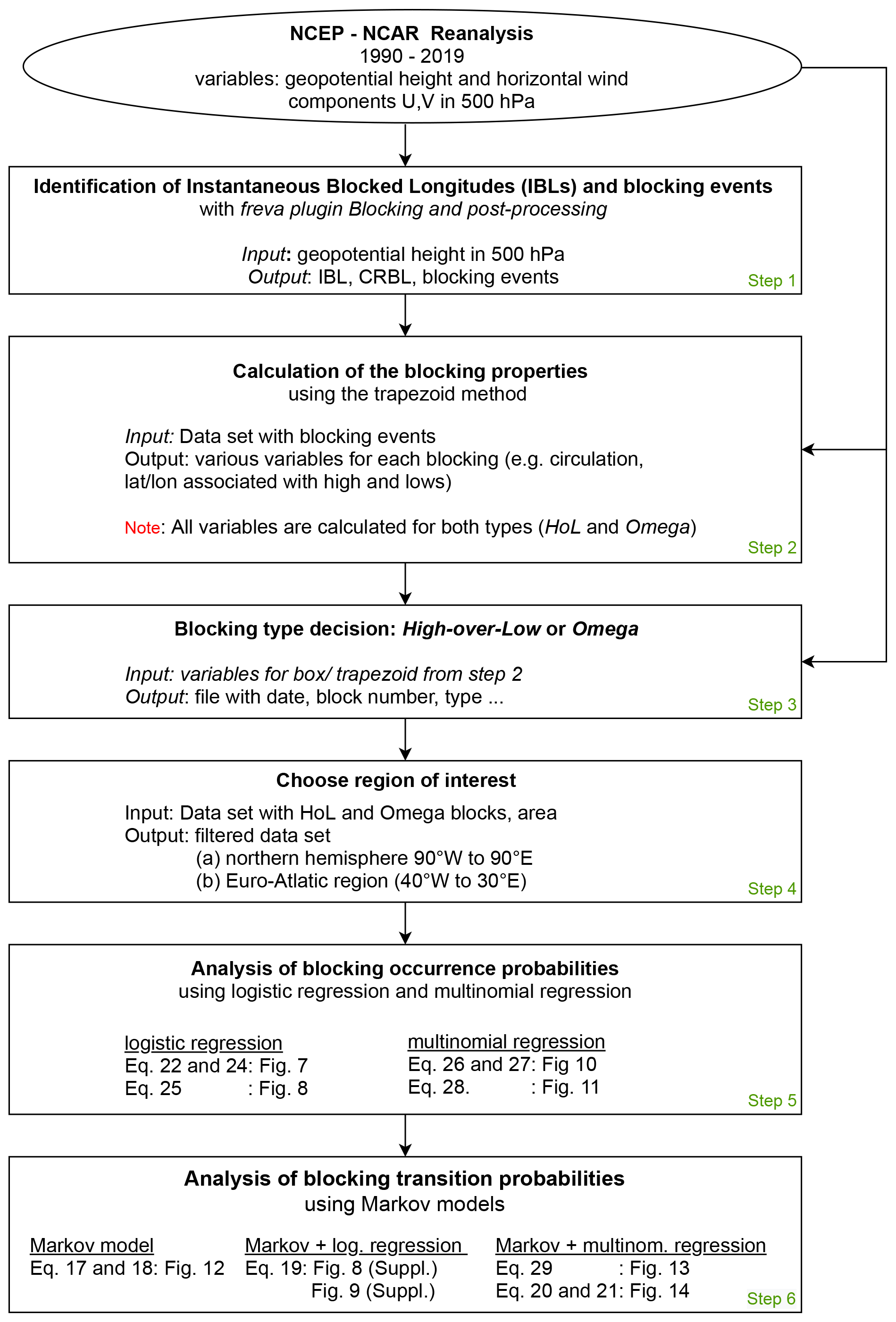
Figure 2Structure diagram of the individual steps of the evaluation as explained in Sect. 3.
3.1 Step 1: identification of instantaneous blocked longitudes (IBLs) and blocking events
In the first step, we use the Blocking plugin (Richling et al., 2015) of the Freva system (Freie Universität Berlin Evaluation System; see Freva, 2017; Kadow et al., 2021) to calculate the so-called instantaneous blocking index. This index is a binary 1D blocking index that determines instantaneous blocked longitudes (IBLs) for every time step of a data series. The IBL was developed by Tibaldi and Molteni (1990) and identifies blocks in terms of gradients of the geopotential height with regard to a central reference blocking latitude (CRBL). While the CRBL is fixed to 50∘ N in the original work, the Freva blocking plugin uses a modification (after Barriopedro et al., 2010) that allows for a longitudinally dependent, temporally varying CRBL in accordance with the climatological storm track. A blocking is identified if the geopotential height gradients on the northern (GHGN) and on the southern (GHGS) side of the CRBL satisfy the following criteria (following Richling et al., 2015):
where Z is the geopotential height at 500 hPa, and the latitudes are given as , and . Here, δϕ is set to 15∘ latitude. Here, the spatio-temporally varying CRBL ϕC is determined based on the 30-year climatology (1990–2019) of the 500 hPa geopotential height field. In order to capture blocking that is not directly located at the CRBL, a possible shift Δ to the north and south is set to 10∘ latitude. For each time step, we obtain a binary value for all longitudes (1: blocked; 0: unblocked). For more details on the method see Richling et al. (2015), and for the specific configurations used in the analysis see the Supplement.
Prior to the blocking classification, the time series of IBLs is post-processed in the following manner: first, we identify blocking events as simply connected points of IBL=1 in the time–longitude field. Then we chose events with a minimum duration of 5 d, i.e., 20 time steps, and a spatial extent of at least 15∘ longitude. We only consider Northern Hemisphere blocks in the longitudinal range of 90∘ W to 90∘ E and north of about 45∘ N. Note that two blocking events can exist at the same time in different parts of the area since the region is very large. In this case, only the first blocking is considered for the subsequent analysis. Further blocking events are discarded since only one state can be used per time step.
3.2 Step 2: calculation of the blocking properties with the trapezoid method
Based on the blocking event list from Step 1, we now search for blocking patterns in the corresponding NCEP–DOE Reanalysis fields with the trapezoid method (Müller et al., 2015; Hirt et al., 2018) to detect high-over-low and omega blocking patterns. This approach uses aspects of flow kinematics to identify the vortices as well as point vortex theory to determine blocking properties and to classify the blocking type. In a regular latitude–longitude projection, a high-over-low block can be outlined by a rectangle (or box) surrounding the high and the low; an omega block instead can be outlined by a trapezoidal shape, where the two lows form the broader base of the trapezoid and the high its smaller top. By assigning specific parts of the trapezoid or box to each low and high, we are able to determine the properties (circulation, location of vortex center) of the associated vortices (see Fig. 3 of Müller et al., 2015). The trapezoid method as it is used here is based on the method introduced in Hirt et al. (2018) with slight modifications. The reader is referred to their publication for more details. We give a brief overview of the method in the following.
The highs and lows are detected by an analysis of the kinematics of the flow. Therefore, we use the dimensionless kinematic vorticity number (Truesdell, 1953, 1954), which compares the local rotation rate and strain rate at each grid point. Here, and denote the anti-symmetric and symmetric components of the velocity gradient tensor ∇v that describes the kinematic flow properties around a point. In our case, represents the horizontal wind vector.
For two-dimensional flow in spherical coordinates with longitude , latitude and Earth's radius R, the kinematic vorticity number is proportional to the magnitude of the horizontal deformation, where
The vertical component of relative vorticity ζ (called vorticity from now on) is given as
For the calculation of Wk, we use the two-dimensional, horizontal wind components of the NCEP–DOE Reanalysis data set at the 500 hPa level. A vortex is then defined as a region of Wk>1, i.e., as an area where the rotation rate prevails over the strain rate (see Schielicke et al., 2016; Schielicke, 2017, for further insight and more atmospheric applications). Otherwise, the Wk values at all grid points where Wk≤1 are set to zero to obtain a field of vortex patches. This field can then be multiplied with another field of interest, for example the vorticity field, to get areas of positive and negative vorticity, i.e., cyclones and anticyclones in the Northern Hemisphere. In this field, we search for the anticyclone that lies closest to a duration-weighted IBL2. Inside a box bounded by this duration-weighted IBL ± 15∘ longitude and between 55 and 85∘ N, the grid point with the most negative circulation Pmax,neg is identified first. The circulation of a grid point i is calculated as
where ζi is the vorticity at that grid point, and Ai is the area associated with grid point i. It is negative (positive) if the vorticity is negative (positive). The circulation of the high ΓH is calculated as the sum of all grid points N with negative circulation inside a radius of 1500 km around Pmax,neg as
The radius of 1500 km was chosen following Hirt et al. (2018), who did a sensitivity study to find the optimal radius that represents the circulation magnitude of the high. Therefore, Hirt et al. (2018) started with a smaller radius of 500 km around the high centroid and increased the size gradually by 250 km steps up to 3000 km. They observed that the circulation magnitude stabilizes around a radius of 1500 km, which was then chosen as a threshold (see Hirt et al., 2018, for more details). Moreover, the Rossby radius of deformation in a stably stratified; dry high is indeed larger compared to a less stable low-pressure system because of the larger Brunt–Väisälä frequency. This further supports the choice of 1500 km.
Similar to the definition of the circulation centroid of a vortex system in point vortex theory, the circulation centroid of the real, extended high is defined as (see also Hirt et al., 2018)
where xi is the horizontal coordinate vector of grid point i, and N is defined as above. Note that the (positive) circulation and the circulation centroid of a low are calculated in a similar way. The coordinates (CH,x, CH,y) of centroid CH are finally used to define the rectangle that encloses the high by a fixed distance ( km, km), which accounts for the typical length scale of a high in the mid-latitudes and allows for some deviations from a pure circular shape. The rectangle that encloses the high is then extended equatorwards by steps of 2.5∘ latitude up to 20∘ N. These boxes are then compared to identify the box that minimizes the total circulation within the box. The total circulation is defined as the sum of the negative circulation associated with the high and the positive circulation associated with the low. However, only grid points with negative circulation northwards of the low centroid and positive circulation south of the high centroid are taken into account for the calculation of the total circulation. This box outlines the high-over-low configuration. At the same time, we search for a minimum of total circulation within a trapezoidal shape, which represents an omega configuration. To this end, we increase the southern edge of the box symmetrically by steps of 2.5∘ longitude (on each side) up to a total length of 2.5 times the east–west length of the box around the high center. The northern boundary remains fixed, and only grid points whose centers lie within the trapezoidal shape are counted. Again, only certain areas of the trapezoid are attributed to the high (everything north of the mean latitude of the low centers), to the western low (everything south and west of the high centroid) and the eastern low (everything south and east of the high centroid).
Point vortex theory is the basis for this pattern-like identification. It states that a system of two or three vortices moves westward if the sum of their circulations is zero, the high lies poleward of the low(s), and the three-point vortex system forms an equilateral triangle (Müller et al., 2015). Note that we determine the box associated with the high-over-low pattern as well as the trapezoid with the omega pattern for each time step separately. We derive a number of block properties, such as the circulations, the latitude and longitude associated with the high and the lows (centroids), for each pattern. The decision on the blocking type pattern is described in Step 3.
3.3 Step 3: blocking type decision – high-over-low or omega blocking
We inspect the relative vorticity in the area south of the circulation centroid of the high with coordinates (longH, latH) for the blocking type decision. To this end, a rectangle is centered around the coordinate (longH, ), where is the mean latitude of the low centroids that are associated with the omega block pattern at that time step. This rectangle has a latitudinal extent3 of at least 10∘. Its longitudinal extent is bound to the size of the trapezoid. We split this rectangle into three smaller rectangles, where the middle one has a width of 25∘ longitude, and the two outer rectangles are limited by the outline of the trapezoid (see Fig. 3a)4. If the mean vorticity inside the middle rectangle (Box 2 in Fig. 3a) is larger than the sum of the mean vorticity of all three rectangles, we define the time step as a high-over-low block, otherwise as an omega block. This results in a time series containing both blocking types for a single blocking event (for an example see Fig. 3b and the video in the Supplement). This is a new addition to the trapezoid method in Hirt et al. (2018), who assigned a single blocking type to each whole blocking period. Finally, a blocking event is expected to consist of the same anticyclone, and we check if this assumption holds: in order to obtain configurations associated with the same high, we split each blocking period into smaller periods if the distance between the centroid locations of two highs in successive time steps (6 h) is too large (distance criterion). We assume that these two highs represent the same system if the distance is smaller than 10∘ latitude (≈1000 km in north–south direction) and smaller than 15∘ longitude (≈1000 km in west–east direction). Otherwise, we assume that these two highs represent two different systems. This allows for slow motions of the blocks; “large jumps” in distances, however, would rather indicate that a different high-pressure system enters the configuration. If the lifetime of one or both events in the split period is shorter than 5 d, the event(s) is (are) removed from the analysis. This reduces the maximum duration of the blocking periods but is also more consistent with following the blocking as a system of vortices (instead of a weather regime that characterizes a larger region). This rather Lagrangian view of blocking differs from the Eulerian perspective we would get using only the instantaneous blocked longitudes to identify blocking.

Figure 3(a) Schematic representation of the blocking type decision based on the trapezoid method. The positive relative vorticity is calculated for all three boxes, which lie on the mean latitude of the low-pressure areas (L1, L2). Depending on the magnitude of the mean vorticity in these three boxes, the decision between high-over-low and omega is made. (b) An example blocking event, observed from 26 June 2019 at 18:00:00 UTC to 28 June 2019 at 00:00:00 UTC, is plotted for six time steps that include a transition between omega and high-over-low blocking states. Shaded areas represent the identified vortex field (Wk>1), which is colored by relative vorticity (in 10−5 s−1; blue: anticyclonic; yellow: cyclonic). Black contours are isolines of geopotential height in 8 dm intervals (the thick black contour is the 584 dm isoline). The outline of the trapezoid or box is given for each time step; solid shapes represent the identified shape; circles are the circulation centroids of the identified high (red) and low(s) (blue) for the omega pattern. In the same way, crosses are used for a high-over-low pattern. The red bars at the bottom of the figures show the identified IBLs from Step 1. The figures were plotted with the help of Matlab (2016), and coastlines were plotted with the built-in MATLAB file coast.mat. The full time series is given in the Supplement; see also steps 2 and 3.
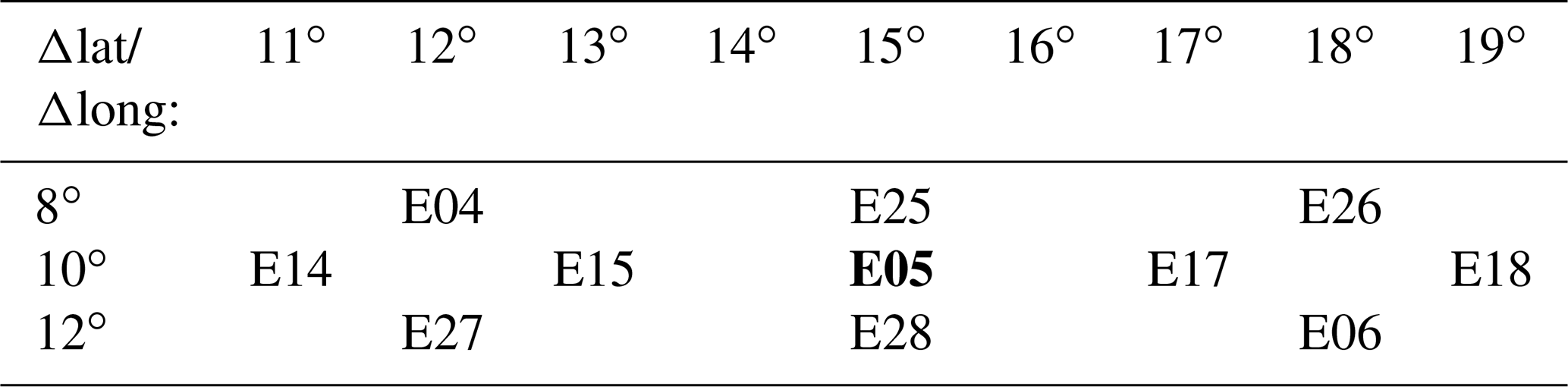
Note that we follow mostly the method described in Hirt et al. (2018), who already tested the sensitivity of the trapezoid method regarding the choice of several parameters. We would like to refer the interested reader to their paper for more details. However, in order to better estimate the effect of the distance criterion that we introduce in this work, we did a number of experiments with different distances (see Table 1). As we intend to bound the distance between high centroids in successive time steps by the typical synoptic-scale Rossby radius LD≈1000 km, all experiments have distances which are close to this value. In Sect. 4, we present results for experiment E05 (see Table 1) with criterion (if not mentioned otherwise).
Table 1Labeling of experiments with different distance criteria that are used to estimate the uncertainty in the blocking identification method. Differences in longitude Δlong and latitude Δlat are given in degrees. Most of the results presented in Sects. 4.2, 4.4 and 5 are based on the E05 setup; hence the entry is highlighted in bold.
3.4 Step 4: choose region of interest – Euro-Atlantic region and half of Northern Hemisphere
Following Step 1 to 3, we are left with blocking events occurring between 90∘ W and 90∘ E with a lifetime of at least 5 d (=20 time steps). High centroids lie in the mid-latitudes between about 44.5 and 83∘ N. To analyze blocking in Europe in more detail, we create a subset: the Euro-Atlantic sector ranging from 40∘ W to 30∘ E. Since this is a subset of the larger blocking event list, blocks with lifetimes smaller than 5 d can occur in this region as at some point in their lifetime, blocks might move in or out of the Euro-Atlantic sector.
3.5 Step 5: analysis of blocking occurrence probability using logistic regression
Logistic regression is designed to model probabilities p (with ) and is thus adequate to describe blocking occurrence probabilities and their temporal changes for a system that can only yield two states: in our case blocking and no-blocking patterns. Occurrence probabilities for a system with three possible states – unblocked, omega and high-over-low – can be analogously described with multinomial regression. Both are briefly reviewed here.
Logistic regression is a special case of generalized linear models (e.g., Wilks, 2011; Dobson and Barnett, 2008) designed to describe occurrence probabilities depending on a set of external influences (covariates). These covariates can be, for example, time in years as a proxy for climate change, the season or month of occurrence as a proxy for the seasonal cycle, or also large-scale atmospheric flow variables.
The setting can be viewed as a generalization to standard linear models. Let Yt be a discrete random variable at discrete times t; observations of Yt are denoted as yt. The random variable Yt describes the discrete states of a Markov chain. We begin our analyses with the two-state model that is based on these two states: no blocking (nB) and blocking (B). Observations (coded in integers) can thus only be yt=0 for nB and yt=1 for B. The random variable Yt follows a binomial distribution completely determined by the expectation value, which gives the occurrence probability of the blocking event . The probability of the state no blocking is determined by the counter-probability .
Logistic regression describes the dependence of the blocking occurrence probability pt at time t as a function of covariates xl,t using a log odds (or logit) link function
with l=1, …, L covariates xl,t observed simultaneously with observations and yt and βl being model parameters to be estimated based on iteratively reweighted least squares (IRLs). Further details can be found, e.g., in Dobson and Barnett (2008); Wilks (2011). We use the function glm() from the package stats of the R environment for statistical computing (R Core Team, 2018).
Rearranging Eq. (8) yields the following expression for the blocking occurrence probability at time t as a function of the covariates xl,t:
In some cases, the influence of one covariate xi,t depends on the value of another covariate xj,t, which can be introduced in a linear model as a so-called interaction effect . Consider, for example, that the change in blocking occurrence probability with years is dependent on the season we are looking at. A simple example with main effects of two covariates and one interaction is
In the notation for generalized linear models introduced by McCullagh and Nelder (1989) Eq. (10) reads
with xi,t denoting main effects, interaction effects and their combination. This notation assumes an offset (β0) being present by default and a parameter βi to be estimated for each term in the equation. Nota bene: in this notation, the symbols “+”, “:” and “*” have special meanings, namely addition of a term in the predictor, interacting effects and combination of both, respectively.
For more than two states, the model can be extended to multinomial logistic regression. We next consider a multinomial random variable Yt with three states: no blocking (nB), high-over-low (HoL) and omega blocking (Ω). For the multinomial distribution, one probability, e.g., , is set as a reference, and the other two ( and ) need to be estimated using
The remaining occurrence probability for no blocking can then be derived as . We thus need to solve two regression equations simultaneously. This can be formulated in the framework of (vector) generalized linear models (VGLMs) (Yee, 2015). Parameter estimation is somewhat more cumbersome in this case, realized using iteratively reweighted least squares and detailed in Yee (2015). Estimation is carried out using the function vglm() from the R package VGAM (Yee, 2015). Confidence intervals (95 %) are based on asymptotic normality of the estimator using an interval [] around the estimator with standard deviation .
3.6 Step 6: analysis of blocking transition probabilities using Markov models
We use Markov models with two and three states to describe transition probabilities between the states related to the different blocking types and the no-blocking state. For both cases, there is thus a discrete set of possible states:
-
two-state model, consisting of blocked (B) and unblocked (nB) states
-
three-state model, consisting of high-over-low (HoL), omega (Ω) and unblocked (nB) states.
The system evolves along a discrete time axis t and can switch between these discrete states. We obtain a discrete-time Markov chain on a finite-state space. The underlying theory was developed by the Russian mathematician Andrey Andreyevich Markov. For the translated original work see Markov (2006).
Let Yt be a sequence of discrete random variables denoting the possible states the Markov chain can be found in; e.g., Yt=i implies Y being in state i at time t. In general i∈{1, 2, 3, …, I}; here, I=2 and I=3 for the two-state-model or three-state-model, respectively. We speak of a transition when changes to Yt=j. Transitions from are described with conditional probabilities which, in general, depend on the history of the process; i.e.,
Formally, is also called a transition from state i to itself. The Markovian assumption (or Markov property) requires these transition probabilities to depend only on the actual state and not the full history of the process:
This assumption makes handling these processes a lot easier. For homogeneous Markov chains, the transition probabilities are independent of external factors or time, i.e., . Otherwise we speak of a non-homogeneous Markov chain. The probability for finding the system at time t in state j, i.e., Pr{Yt=j}, is determined by the transition probabilities pij from all states i into state j weighted with the probability of finding the system in state i; thus
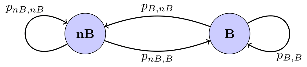
The simplest Markov Chain is a Bernoulli process consisting of two states. In our case, the two-state model with the states no blocking (nB) and blocking (B) (i, ) has the transition matrix
with transition probabilities . For the three-state-model with the states high-over-low blocking (HoL), omega blocking (Ω) and no blocking (nB) (i, ), the transition matrix is
Transition probabilities are between 0 and 1 (), and rows sum up to unity, implying that the probability that any of the possible states' i is reached at time t+1 is one. Transition probabilities together with the probability distribution of Y0 (initial distribution) fully describe the Markov chain.
Homogeneous (time-independent) Markov chains can be illustrated using a network diagram. Figure 4 shows an example with two states. The circles describe the different states, and the arrows indicate the direction of the transition with the corresponding transition probability pij. In the homogeneous case, transition probabilities can be estimated from relative frequencies. A more general description of Markov chains and their matrices of transition probabilities can be found in chap. 9.2 in Wilks (2011). More examples of atmospheric applications of (finite-state) Markov chains can be found in Gottwald et al. (2016, chap. 3.4). For further details on homogeneous Markov processes, see e.g., Baclawski (2008).
For a non-homogeneous (time-dependent) Markov process, we use logistic regression to estimate time-varying transition probabilities. For the two-state model with the two states blocking (Yt=B) and no blocking (Yt=nB), we describe transition probabilities changing with year as
using the notation for generalized linear models as well the parameter estimation strategies introduced above. This results in probabilities for blocking conditioned on being in an unblocked state and conditioned on being in a blocked state varying in time, as do their counter probabilities and . Analogously, we can describe time-varying (with “year” and season “seas” or month “mon”) transition probabilities for the three-state model using multinomial logistic regression, setting the reference to and
Probabilities for all transitions can be derived with the condition . For details on main and interaction effects with categorical terms in the predictor, see e.g., Wilks (2011) and Dobson and Barnett (2008).
The results are divided into four subsections in order to answer the research questions posed in the introduction: (1) whether the blocking occurrence probabilities undergo long-term changes and (2) whether onset (formation), decay (offset) or transition probabilities between blocking types undergo long-term changes. In both cases, we ask if these long-term changes depend on season or month. We start with an overview of blocking properties and explore the uncertainty in the identification algorithm in Sect. 4.1. It follows a description of the temporal development of blocking occurrence probabilities for yearly, seasonal and monthly changes in the two-state Markov model (blocking, no blocking) in Sect. 4.2 and for the three-state Markov model (no blocking, omega, high-over-low) in Sect. 4.3. Section 4.4 discusses the transition probabilities of two and three states for the 30-year period.
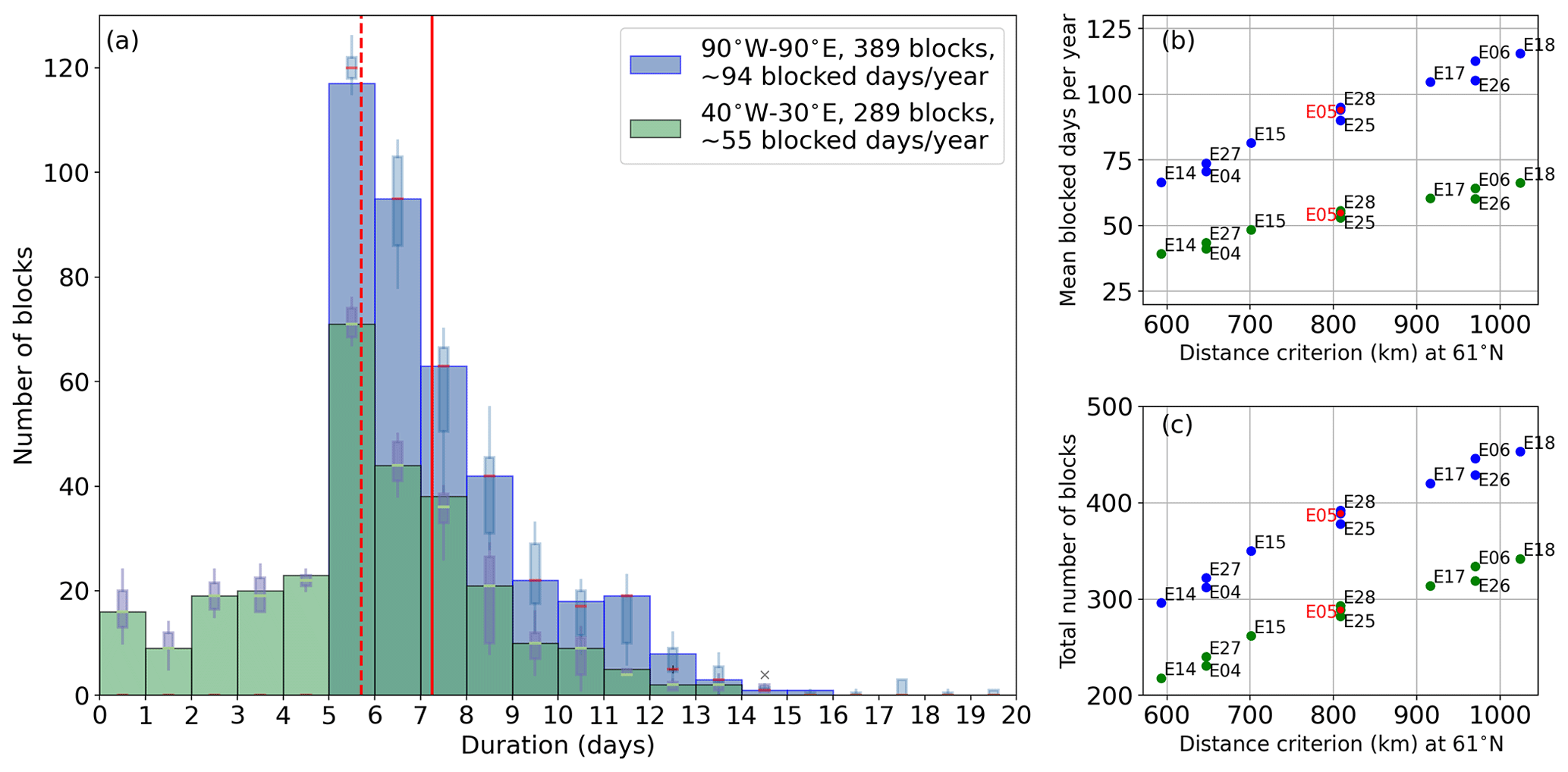
Figure 5(a) Histogram of the duration of all blocking events in the period 1990–2019 for two selected regions. Blue (green) columns represent the region 90∘ W to 90∘ E (40∘ W to 30∘ E) for experiment E05 with a total of 389 identified blocks (289 blocks); solid (dashed) vertical red lines indicate the mean of this data set. Boxplots on top of the bars show the range of the identified block numbers given by different distance criteria (see Table 1). Boxes show the interquartile range (IQR); whiskers indicate 1.5 times IQR; the “x” is an outlier (larger region). (b) Mean blocked days per year and (c) total number of identified blocks in the period 1990–2019 in dependence on the distance criterion. Here the distance criterion was calculated by the longitude criterion of the respective experiments at 61∘ N, which is the mean latitude of all identified highs.
4.1 Uncertainty estimates of the identification method and general overview of blocking properties
A number of experiments with different distance criteria between the high-pressure centroids of subsequent time steps allow us to estimate the sensitivity of the identification method with respect to the distance criterion (see Table 1). The results of these sensitivity experiments are given as a footnote to the results presented. The number of identified blocking events turns out to be sensitive to the distance criterion, with a lower number for stricter (i.e., smaller) maximum distances.
Furthermore, we take a closer look at some general blocking properties such as frequency and duration and their sensitivity to the distance criterion. Generally, the total number of blocks as well as the mean blocked days per year is lower for stricter distance criteria and increases almost linearly with relaxation of the criterion (Fig. 5b and c). The longitudinal distance has a higher impact, while a change in the latitudinal distance criterion only leads to slight differences (e.g., compare experiments E05, E28 and E25 in Fig. 5b and c, which differ by 2 to 4∘ latitude but have the same longitudinal distance criterion).

Figure 6Temporal development of (a, b) blocking number (black) and fraction of annual blocked time steps (green); (c, d) mean (red) and maximum (blue) duration of a blocking event (a, c) for the whole domain (90∘ W to 90∘ E) and (b, d) for the Euro-Atlantic region (40∘ W to 30∘ E). Boxes represent the interquartile range of the experiments described in Table 1 to test the uncertainty in the method for different distance criteria between two time steps. The whiskers are 1.5 times the interquartile range, and single points in appropriate colors represent outliers. Note that blocking numbers are given as integers. Experiment E05 is explicitly plotted in colors corresponding to the boxplots by symbols and lines. These lines are just plotted to ease the identification of E05.
In the 30-year period from 1990 to 2019 in the region 90∘ W to 90∘ E, we detect a total of 389 blocks (≈13 blocks per year) that lasted for 5 or more days (see Fig. 5a, blue columns), with an average of about 94 blocked days per year (92±16 for all experiments). Over all experiments, we observe a mean (± standard deviation) of 381±52 blocks in total in this period (or 12.7±1.7 blocks per year). A total of 289 blocks (284±40 blocks in total for all experiments) out of the 389 blocks affected the Euro-Atlantic region (40∘ W to 30∘ E) for at least some of their lifetime, with an average of about 55 blocked days per year (53±9 for all experiments). Since the Euro-Atlantic blocks are a subset of the blocks that occur in the larger region, blocking lifetimes can be smaller than 5 d. However, only 87 of the 289 blocks remained less than 5 d in the Euro-Atlantic region, while the majority affected the region for 5 to 8 d (153 blocks; see Fig. 5a, green columns). Since blocks are observed to be quasi-stationary with usually low propagation speeds, the small number of short-lived blocks in the Euro-Atlantic region probably start or end close to the region boundaries and move either in or out of the region during their lifetime. The mean duration of the blocks is 7.25 d for the larger region and 5.70 d for the Euro-Atlantic region (vertical red lines in Fig. 5a). Considering all experiments, the mean duration is 7.19±0.30 d for 90∘ W to 90∘ E, and 5.62±0.15 d for 40∘ W to 30∘ E; i.e., the variability in the mean duration is only about one time step (6 h) between all considered experiments. The interquartile range (IQR; purple boxes in Fig. 5a) of the different experiments remains relatively consistent up to a duration of 8 d for the Euro-Atlantic region, with IQR=5.3 blocks per class. For this region, the largest disagreement between the experiments is found for blocks with a duration between 8 and 9 d, with IQR=16.5 blocks. Interestingly in the larger region, the lowest IQR of four blocks is found in the class with the highest block number, with a duration between 5 and 6 d. In all other classes, the experiments differ more strongly with IQR≈12 blocks on average for lifetimes between 6 and 12 d. The number of blocks is sensitive to the distance criterion (Fig. 5c), which leads to splits of blocking events of the IBL-detected blocking periods into two or more smaller periods and can hence increase (or decrease if the new periods are less than 5 d) the overall number of blocks. In terms of averaged blocked days per year (Fig. 5b), the standard deviations are 16 d for the larger region and 9 d for the smaller one. These values account for a fraction of 0.05 and 0.025, respectively, of additional (or fewer) blocked days per year.
The temporal development of the annual blocking frequency and duration for the larger and the smaller Euro-Atlantic region is shown in Fig. 6. For both regions, clear upward or downward trends in blocking frequency over the 30 years are not obvious. However, inter-annual variability is high; see black squares in Fig. 6a and b. Variability between different experiments is relatively large. This spread does, however, not show trends over time; see gray boxes in Fig. 6a and b5. Considering the fraction of blocked time steps per year (green, Fig. 6a and b), the inter-annual variability is still obvious. However, the spread between the experiments is smaller. There is no obvious trend, neither in the values of experiment E05 (corresponding to the lines in Fig. 6) nor in the spread over all experiments. However, the spread is smaller in the Euro-Atlantic region (Fig. 6b) compared to the larger region (Fig. 6a).
The mean duration of blocking events shows a small inter-annual and inter-experimental variability compared to the maximum duration (see red and blue crosses and bars in Fig. 6c and d). Note that the maximum is given by only one data point per year and experiment. The spread between experiments is thus very large in both regions, whereas it is smaller for the Euro-Atlantic region. Note that the residence time of blocks in the smaller region also depends on the propagation speed of the blocking, and a larger variability in the mean duration could be caused by a year-to-year variability in faster or slower propagation speeds.
4.2 Temporal development of blocking probabilities – two-state blocking model
We investigate the inter-annual variability in blocking occurrence probability taking only two states into account: blocking and no blocking; both omega and high-over-low blocks are for now considered to be blocking. Starting with annual probabilities, we resolve the blocking occurrence seasonally and monthly in further steps.
4.2.1 Annual blocking probability
We study annual blocking occurrence probability with logistic regression as described in Sect. 3.5 using
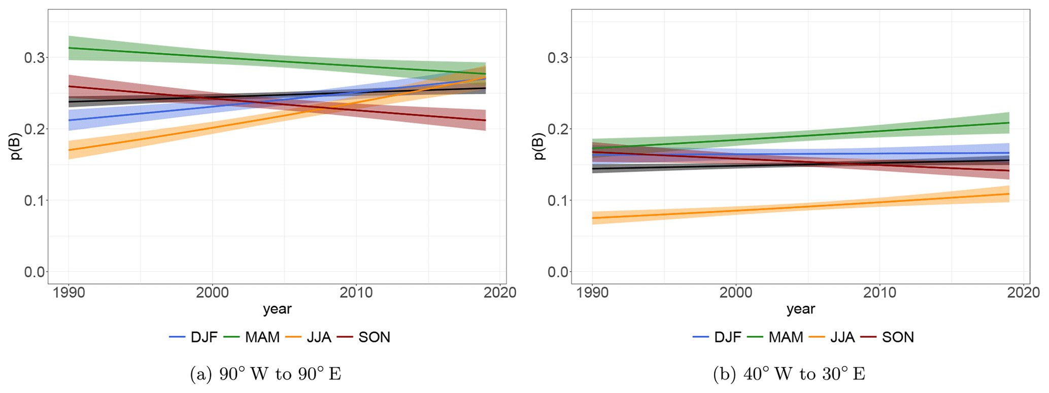
The black lines in Fig. 7 show the model's expectation for the probability that a time step is part of a blocking event that lasted a minimum of 5 d (blocking occurrence probability) for 90∘ W to 90∘ E (Fig. 7a) and the Euro-Atlantic region (40∘ W to 30∘ E; Fig. 7b). Shading gives 95 % confidence intervals. We use a Wald test (z test) to test for a significant trend with years, with p values encoded as
We find an increase of 2 percentage points () for the large region and 1 percentage point (*) in the North Atlantic region. The average probability is about 25 % blocked time steps between 90∘ W and 90∘ E and about 15 % blocked time steps between 40∘ W and 30∘ E. This is in accordance with the fraction of blocked time steps per year plotted in Fig. 6a and b.
4.2.2 Seasonal blocking probability
The colored lines in Fig. 7 show analogously the expectation resolved by season obtained with a model with interactions (Eq. 24)
with being a categorical term in the predictor. The months December, January, February, etc. have been abbreviated by capital letters D, J, F and so forth. The seasonal resolution now allows us to assign the increase for the region 90∘ W to 90∘ E over the 30 years to a large extent to a significant increase in occurrence probability of blocked time steps in summer (JJA) () and winter (DJF) (). During spring (MAM) (*) and autumn (SON) () occurrence probability is decreasing (see Fig. 7a).
In the Euro-Atlantic region, the occurrence probability increase is weaker in summer (JJA) () and not significant in winter (DJF) ( ). However, we observe now an increase in probability also in spring (MAM) (); in autumn (SON) ( ) the slight decrease is not significant. The difference between the two regions suggests that the occurrence behavior of blocking is not the same across the larger region 90∘ W to 90∘ E.
4.2.3 Monthly blocking probability in the Euro-Atlantic region
We now break down trends in occurrence probability in the Euro-Atlantic sector to a monthly resolution using a categorical term for the month mon∈{1, 2, 3, …, 12} in the predictor, interacting with year
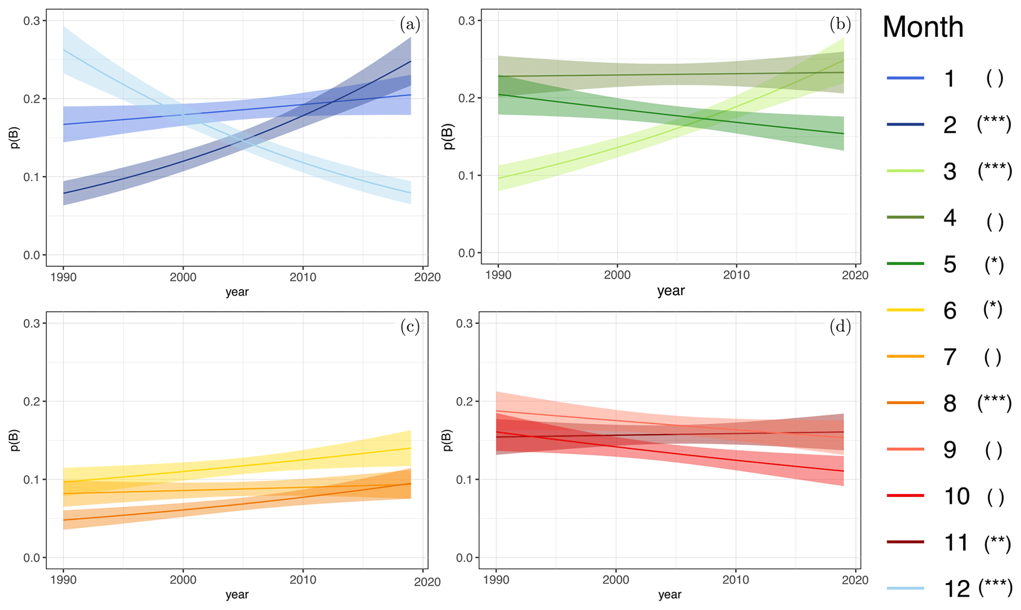
Figure 8Blocking probability over time for individual month (Eq. 25). Shading shows 95 % confidence intervals. (a) Winter (DJF), (b) spring (MAM), (c) summer (JJA) and (d) autumn (SON) in the Euro-Atlantic region (40∘ W–30∘ E). Significance is encoded as , , , .
Figure 8 shows monthly resolved trends in blocking occurrence probability for the Euro-Atlantic region. Figure 8a suggests that a strong decrease in December () compensated by a strong increase in February () and a weak increase in January ( ) results in the approximately constant occurrence probability shown in Fig. 7b. Similarly, in Fig. 8b we see that the strong increase in blocking probability in March () is partly offset by a weaker decrease in May (*), while April is approximately constant. This is consistent with the increase visible for spring in Fig. 7b. The summer months June (*) and August () exhibit an increase in blocking occurrence probability; the change in July is not significant (Fig. 8c). This consistent increase adds up to the significant increase observed for summer in Fig. 7b. In autumn, we see a decrease in November () and non-significant changes for September and October (Fig. 8d). This is reflected in the slight and not significant increase seen for autumn in Fig. 7b. Moreover, all experiments with different distance criteria agree on the decrease in December and the increases in February, March and August.
The consistency between seasonally and monthly resolved results gives confidence in the analysis. Furthermore, it seems worth looking at both resolutions as strong monthly resolved signals can average out when aggregated to the season as in winter, or weak but consistent monthly signals can add to a stronger seasonal signal as in summer. The monthly resolution now allows us to postulate that in the Euro-Atlantic region there are signs for blocking occurrence probability increases at the beginning of the year (JFM) and decreases towards the end of the year (SOND); inter-annual variation in between is comparably small.
4.3 Temporal development of blocking probabilities – three-state blocking model
We now additionally distinguish between the two blocking types high-over-low and omega, considering occurrence probabilities for three states in a multinomial logistic model.
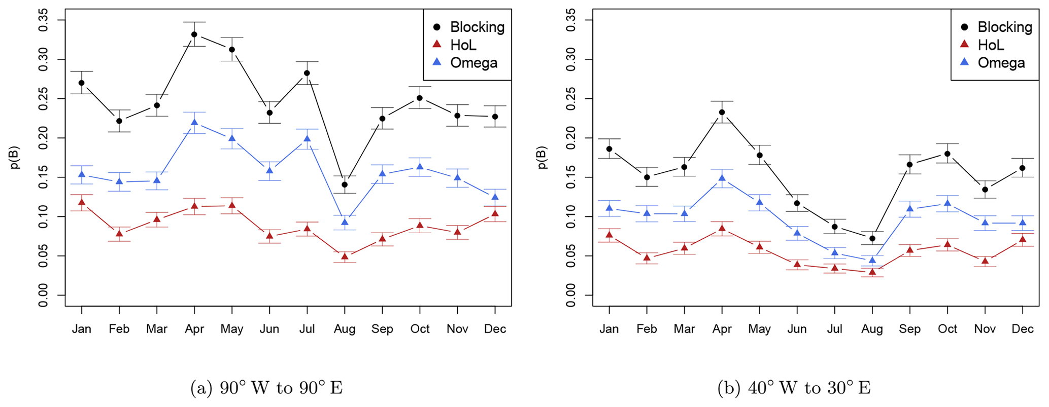
Figure 9Blocking probability estimated for individual months for blocking in general as well as separately for high-over-low and omega. (a) Whole domain (90∘ W to 90∘ E) and (b) Euro-Atlantic subsection (40∘ W to 30∘ E). Whiskers show 95 % confidence intervals assuming Gaussian asymptote for estimating binomial probabilities.
4.3.1 Annual cycle of blocking probability
Taking a look at the annual cycle of blocking probability reveals that the colder months from September to March are characterized by blocking probabilities of about 22 % (≈15 %) between 90∘ W and 90∘ E (40∘ W to 30∘ E), with a smaller peak in January (see Fig. 9). The main peak in both regions occurs in April. While the larger region (90∘ W to 90∘ E) shows a broader peak with high values also in May and a secondary peak in July, in the Euro-Atlantic region the blocking probability only peaks in April and shows a broader minimum in June to August. In the larger region, the lowest blocking probability occurs in August, too, but June and July have higher probabilities. In general, about of the blocked time steps can be classified as omega blocks and about as high-over-low blocks. Only in December and January does this classification change to about (both regions; red and blue triangles in Fig. 9). Note that a blocking does not have to occur in every month of every year (see Figs. S6 and S7). The occurrence frequency of omega blocks shows a larger intra-annual fluctuation (see Figs. S6 and S7 for more details). It is possible that only a few time steps of a blocking lie in 1 month, while the other time steps are in an adjacent month.
4.3.2 Seasonal blocking probabilities in the Euro-Atlantic sector
Having now three states with distinct high-over-low and omega blocks, we use multinomial logistic regression (Sect. 3.5) with reference to . The basic model is given by
using two equations: one for Pr{Yt=HoL} and one for Pr{Yt=Ω}. This can be straightforwardly extended to seasonally resolved trends by
To avoid problems with significance testing due to the Hauk–Donner effect (Yee, 2015, chap. 2.3.6.2), we avoid the Wald test in favor of a likelihood-ratio test. This implies that we test the null hypothesis of constant probabilities against the alternative with probabilities depending on the covariate year. Consequently, we cannot infer significant trends in occurrence probability individually for high-over-low or omega.
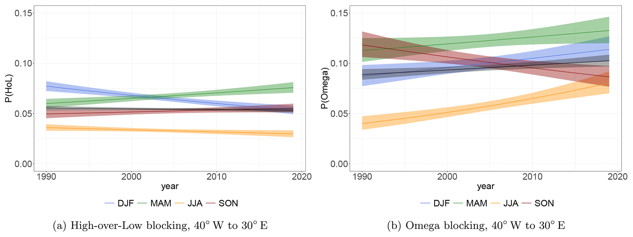
Figure 10 shows the expectation of the multinomial model (Eq. 27) for the temporal evolution of the probabilities of the two blocking types for annual occurrence probabilities (black line) and broken down to seasons (colored lines). Annual occurrence probabilities are constant for high-over-low and slightly increase (*) for omega. In winter, we observe a significant () decrease in high-over-low (Fig. 10a), which is offset by an increase in omega (Fig. 10b)6, leading to almost constant overall blocking in that season (Fig. 7b). The overall increase in blocking probability in spring, seen earlier in Fig. 7b, can now be attributed to a significant (*) increase in both high-over-low and omega blocking; see Fig. 10. In summer (), a strong increase in omega occurrence probability is partly offset by a decrease in high-over-low, leading to a significant increase in summer blocking occurrence in Fig. 7b7. The weak autumn decrease in total blocking occurrence in Fig. 7b can now be attributed to a strong () decrease in omega blocks, which is only partly offset by an increase in high-over-low occurrence (Fig. 10)8.
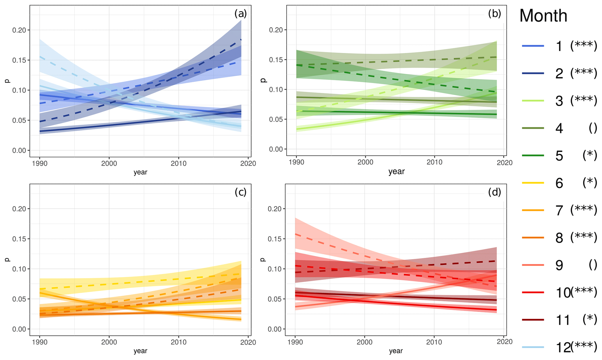
Figure 11Blocking probability over time for individual months (Eq. 28) for high-over-low (solid) and omega (dashed) blocking. Shading shows 95 % confidence intervals. (a) Winter (DJF), (b) spring (MAM), (c) summer (JJA) and (d) autumn (SON) in the Euro-Atlantic region (). Significance is encoded as , , , .

4.3.3 Monthly blocking probability in the Euro-Atlantic sector
We now estimate monthly resolved trends in blocking occurrence probabilities for the three-state model in Eq. (28).
Figure 11 shows the expected occurrence probabilities for high-over-low (solid lines) and omega (dashed lines) blocking resolved by month. Significance from a likelihood-ratio test is again given in the legend of the plot. The probabilities of omega and high-over-low agree on the decrease in December and increase in February, consistent with Fig. 8a; in both cases the trend for omega blocks is stronger. In January, the increase in omega is partly offset by the decrease in high-over-low, leading to a slight increase in total blocking for this month (Fig. 8a). Figure 11b shows that omega and high-over-low occurrence probabilities increase simultaneously in March and decrease simultaneously in May, being consistent with the trends of total blocking occurrence in that month (Fig. 8b). April shows weakly increasing (omega) and decreasing (high-over-low) trends averaging out to almost constant total blocking (Fig. 8b). Figure 11c shows a weak increase in June (*) and August () occurrence probability for both blocking types, consistent with the weak increase in total blocking shown in Fig. 8c. In July (), high-over-low is decreasing, while omega is increasing, resulting in very weakly increasing total blocking probability (Fig. 8c). In October, both blocking types decrease () consistently as well as the overall blocking probability. In September ( ) omega decreases, while high-over-low increases and vice versa in November (*), both leading to almost constant total blocking occurrence probability in the 2 months; see Fig. 8d.
4.4 Transition probabilities
We conceive the dynamics between different blocking and no-blocking states as a stochastic process with Markov properties (see Sect. 3.6). We can thus give transition probabilities for the two- and three-state model in the Euro-Atlantic region. We start with assuming a homogeneous Markov process and give stationary transition probabilities. In a second step, we allow transition probabilities to vary with years. Analogously to the model presented in Sect. 4.3.2, we break the trends in years down to the four seasons.
4.4.1 Transition probabilities of two- and of three-state models
Within the framework of homogeneous Markov processes, we estimate stationary transition probabilities. Figure 12 visualizes the transition matrices for the two-state model (no blocking and blocking) in panel a and the three-state model (no blocking, high-over-low and omega block) in panel b. The estimate for the transition probability from no blocking to blocking is , denoting that in about 1 % of all time steps (6 h resolution) we observe an onset of blocking. Being in a blocked state, we estimate the persistence to remain in this state as and the decay to a non-blocked state as . Thus, being in a blocked state, the probability to remain (persistence) there is about 94 %, and the probability that this blocking decays is about 6 %. Being in the no-blocking state, we find a probability to remain there of .
Considering the three-state model, we can now break down the total blocking onset probability into the onset of high-over-low () and the onset of omega (). Thus in about two of three blocking onsets, we see an omega blocking rather than a high-over-low9. This does not hold for the offset as in the three-state model offset probability is conditioned on omega or high-over-low. Furthermore, we see two indications for omega blocks being more stable than high-over-lows: (i) the persistence of omega blocking is with larger than the persistence of high-over-low (), and (ii) the transition from high-over-low to omega is with larger than the reverse transition with . Probability estimates and standard errors are given in Tables 2 and 3.
Table 2Probability estimates ± standard errors (SE) for the two-state model. Probabilities give the transition to the state given in the column conditioned on the state given in the row.
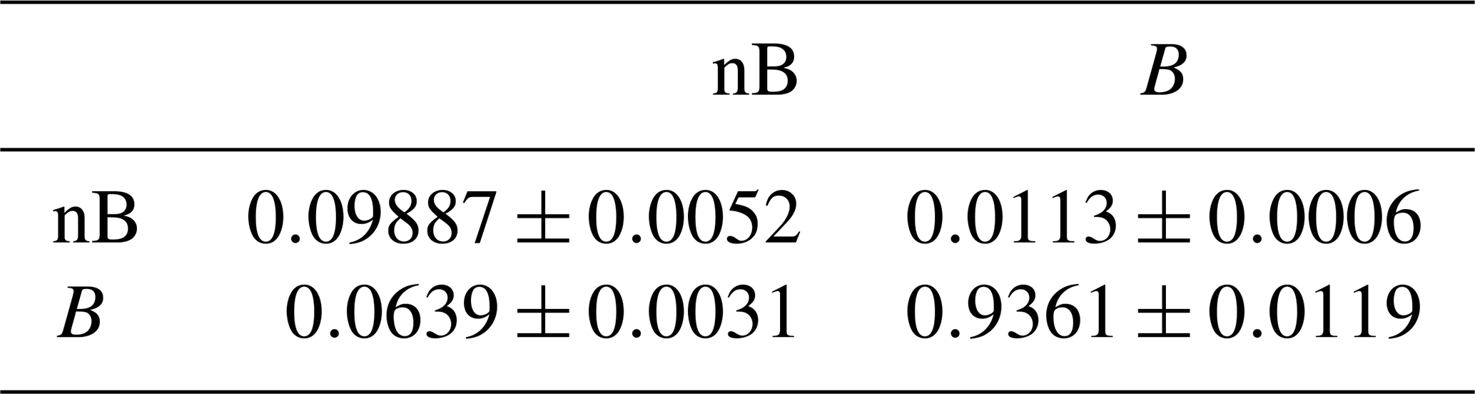
Table 3Probability estimates ± SE for the three-state model. Probabilities give the transition to the state given in the column conditioned on the state given in the row.
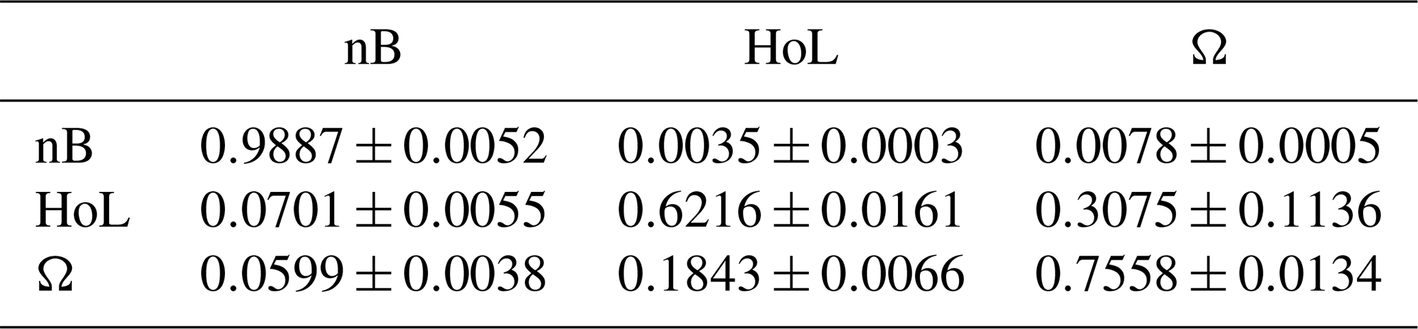
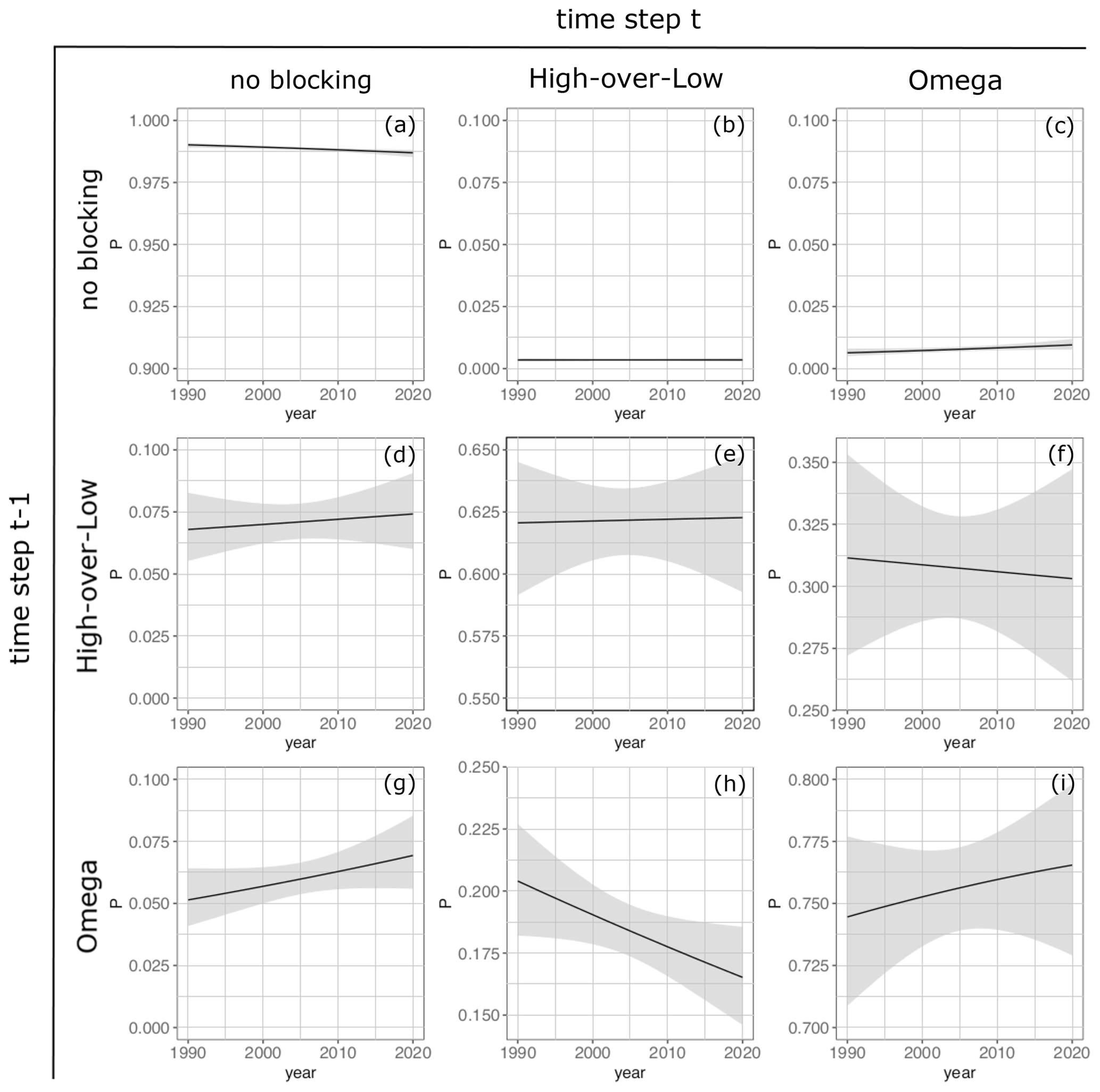
Figure 13Transition probabilities analogous to the matrix of a three-state Markov process (Eq. 18) as a function of years (Eq. 29) in the Euro-Atlantic region (40∘ W–30∘ E); (a) pnB|nB, (b) pHoL|nB, (c) pΩ|nB, (d) pnB|HoL, (e) pHoL|HoL, (f) pΩ|HoL, (g) pnB|Ω, (h) pHoL|Ω and (i) pΩ|Ω. Shading shows 95 % confidence intervals.
4.4.2 Trends of transition probabilities of two- and of three-state models
We describe the change in transition probabilities with time (years) using logistic and multinomial regression on the annual timescale and broken down into seasons. For the two-state Markov model (Eq. 19) no significant changes can be identified, neither for the full annual probabilities nor broken down into seasons; see Figs. S8 and S9. Changes in transition probabilities for the three-state Markov model with annual occurrence probabilities are described by
Figure 13 shows the temporally varying transition probabilities for the three-state model as a function of the year. Rows and columns are arranged analogously to the transition matrix (Eq. 18, Table 3); shading gives 95 % confidence intervals. Analogously to Sect. 4.3.2, we use the likelihood-ratio test to infer whether inclusion of the trend in years results in a significantly better model than the homogeneous Markov process. With a p value < 0.05 we find significance on the 5 % level. Besides the first row, confidence intervals are larger than the signal itself, and we refrain from detailed inferences on the trends for transitions from the two blocking states high-over-low and omega. However, we can see a positive trend for the transition from no blocking to omega (Fig. 13c) and a consistent decline in the persistence of no-blocking states (Fig. 13a), while the transition from no blocking to high-over-low is approximately constant (Fig. 13b). This is in line with (i) the slight increase in overall blocking probability (Fig. 7b, black line) and (ii) the increase in omega blocking (Fig. 10b, black line). It further indicates that omega blocking is more favored for a blocking onset towards the end of our study period.
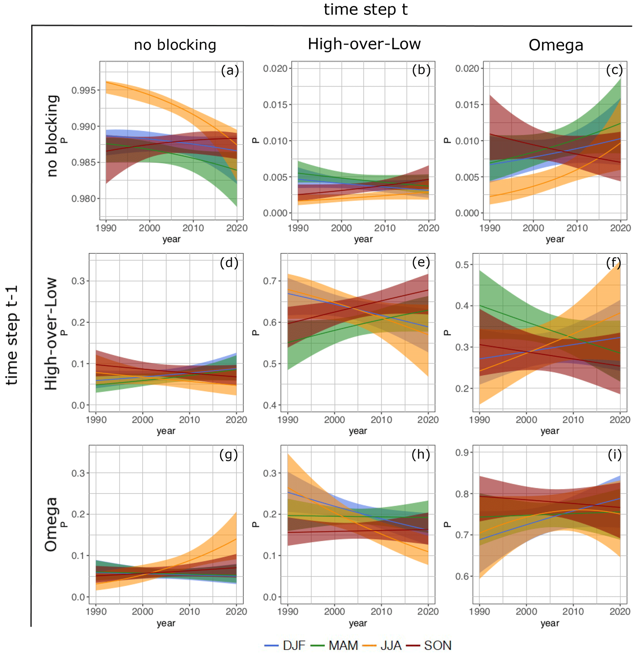
Figure 14Transition probabilities analogous to the matrix of a three-state Markov process (Eq. 18) as a function of years for individual seasons (Eqs. 20 and 21) in the Euro-Atlantic region (40∘ W–30∘ E). Panels are ordered analogously to Fig. 13; season is color-coded. Shading shows 95 % confidence intervals.
We now use the model given in Eqs. (20) and (21) to break the previous results down into seasons. Analogously to Fig. 13, Fig. 14 shows trends in transition probabilities with lines colored according to the season.
Inclusion of the trend in years broken down to seasons is – according to the likelihood-ratio test – a significant improvement over a homogeneous Markov process for summer – JJA, (), winter – DJF, (*) and spring – MAM, (*); for autumn (SON), improvement is not significant on the 5 % level. Figure 14c now suggests that the previously observed increase in blocking onset to omega (Fig. 13c) is strongest in summer, weaker in spring and winter, and even reversed in autumn. This is consistent with the negative trend in the probability to remain in a no-blocking state being strongest in summer (Fig. 13a). For most other cases, the confidence intervals are so large that they are also consistent with constant probabilities. Detailed interpretation is thus to be taken with care. Having said that, Fig. 13e suggests that high-over-low becomes slightly more stable in spring and autumn and less stable in summer and winter; stability for omega is even less clear to determine from Fig. 13i; however a slight increase in winter and decrease in spring can be observed (in both cases confidence intervals are compatible with a constant transition probability). Further interesting aspects are changes in transition probabilities from omega to high-over-low and vice versa. These are difficult to infer based on the data set used here (large confidence intervals). However, there seems to appear a slight increase in transitions from high-over-low to omega in winter and summer; the opposite transitions in winter and summer decrease. Furthermore, the transition from high-over-low to omega shows a slight decrease in spring and autumn and the opposite transition a slight increase. Although inference is difficult here, these results are consistent with the significant increasing (decreasing) occurrence probability of omega (high-over-low) blocking in summer and winter (Fig. 10).
Point vortex theory and the kinematic vorticity number allow us to automatically classify atmospheric blocking into high-over-low and omega blocking; the two types are distinguished by the position of the associated low-pressure system(s). These positions are of general importance as the associated blocking types can affect and impact different regions due to their different structures. A key element is the Lagrangian framework, within which we require the high-pressure system to remain the same vortex over the whole lifetime of the system. We do, however, allow for local variations in and replacements of the low(s). This distinguishes our approach from other studies that rather focus on blocking as a large-scale weather regime within a defined region (Eulerian perspective). We thus refine the method developed by Hirt et al. (2015) to identify and distinguish omega and high-over-low blocking. With logistic regression we describe occurrence probabilities for blocking and blocking types and identify potential trends in these broken down for individual seasons and months. This is finally extended with Markov models, giving additional transition probabilities between blocked and unblocked states.
5.1 Discussing the two-state model
Investigating blocking without the distinction of omega and high-over-low, we see a slight increase in annual occurrence probability in both regions (Fig. 7, black lines). A low probability of blocking in the summer months in the Euro-Atlantic sector is clearly recognizable. Tyrlis and Hoskins (2008) and Brunner et al. (2017) show similar results regarding the blocking minimum in summer. This minimum can be explained by the variation in the pressure anomalies. In spring and autumn the amplitudes of the pressure anomalies are larger than in summer (see e.g., Wallace et al., 1993). Therefore, the high- and low-pressure systems are more distinct and can last longer. Allowing for different trends in each season reveals increasing trends in occurrence probabilities in summer and winter and decreasing trends in the transition seasons for the larger region (90∘ W–90∘ E). These opposing trends add up to the slight increase for the full year. In the Euro-Atlantic region we see an increase in spring and summer and weaker trends for the other seasons, again summing up to a weak trend for the full year (Fig. 7, colored lines). This difference among the two regions implies that the seasonal dependence of trends varies regionally. The increasing blocking trends in summer support the authors' perception that occurrences of exceptional droughts that were experienced 2018 and 2019 in central Europe (Hari et al., 2020) are likely to occur more frequently at the end of our study period than at the beginning. A further breakdown to individual months for the Euro-Atlantic region reveals that an investigation of trends for a season is not necessarily the best choice to identify changes. While in summer, the trends in occurrence probability are all positive (adding up to a strong positive summer trend), monthly resolved trends in winter, spring and autumn are not in agreement and weaken the seasonal signal (Fig. 8). Particularly the late winter/early spring (February/March) blocks can have a significant impact on the vegetation and on agriculture in general since they are often connected to temperature extremes. For example, Brunner et al. (2017) found a strong link between cold spell days in February and co-occurrence of blocking and a link between warm spell days and blocking in late spring in Europe, but they found “no apparent trend in the number of blocked days”. However, their study focused on temperature extremes and not on blocking trends, and their identification method differed from ours. Nonetheless, we find a significant increase in blocking occurrence probability in February and March.
In their work on observed blocking trends during the time period 1980–2012, Barnes et al. (2014) found the following: “No clear hemispheric increase in blocking is evident in any season for any blocking index, although robust seasonal increases and decreases are found for isolated regions.” We can partly confirm this statement: although we find significant trends regarding the seasons, these trends are small and depend on the region.
5.2 Discussing the three-state model
Distinguishing between omega and high-over-low blocking, we find occurrence probabilities of omega blocking being larger than of high-over-low (Figs. 9–11). Both types exhibit a different trend in annual occurrence probabilities. While the occurrence probability of high-over-low blocking remains about constant in the study period, a slight increase can be seen for omega blocking (Fig. 10, black lines). Resolving these trends seasonally amplifies the difference between the two types: while occurrence probabilities for high-over-low show a slight decrease in summer and winter and increase in the transition seasons (Fig. 10a, colors), occurrence probabilities for omega decrease only in autumn and increase in the other seasons, leading to an overall increase (Fig. 10), colors). A further breakdown of trends for individual months allows for an even more detailed investigation: within one season, the monthly resolved trends do not necessarily agree, as we found for the two-state model. The three-state model now reveals whether a specific type is contributing to changes in blocking occurrence probability or if there are opposing changes for both types, leading to minor or no change in overall blocking. Strong trends can be observed for omega blocking occurrence probability for all 3 winter months, decreasing in December and increasing in January and February; trends are weaker for high-over-low and even opposing in January (Fig. 11a). In spring, monthly resolved trends agree among both types, especially on the increasing trend in March. This reflects the overall blocking trends given in Fig. 8b and the seasonal type-specific trends in Fig. 10. Trends in July disagree for omega and high-over-low, with the latter decreasing. This results in the small change (non-significant) for overall blocking shown in Fig. 8c. In autumn, we see strong and opposing trends in September and weak opposing trends in November (Fig. 11d). Both lead to (almost) vanishing trends for overall blocking (Fig. 8). For October, both types behave consistently with overall blocking. In some cases, we have thus seen the necessity to be able to distinguish blocking types and also to model trends for individual months. Otherwise, we would – in some cases – remain with the impression of (almost) constant blocking occurrence probabilities as shown in Figs. 7 and 8 for some seasons or months. The description of type-specific and monthly resolved trends suggested here is important, particularly as the location of the associated lows differs between types, and therefore their impact does to. Hence with respect to warm and cold spells in early spring and for heat waves in summer, this distinction between the blocking type is especially relevant to society and should be studied further. However, adding more detail to the analysis by considering blocking types and individual months leads on the one hand to larger uncertainties as more model parameters are needed to be estimated, but on the other hand, this might also lead to stronger signals, making statistically significant results possible.
5.3 Discussing transition probabilities for the two-state model
Within the two-state model, the probability of remaining in a blocked state for the next 6 h is (Table 2 and written at the associated arrows in Fig. 12a). The onset probability, i.e. the transition from the state no blocking to blocking, is much lower (), and so is the decay probability . Spekat et al. (1983) found daily transition probabilities for the onset of a meridional weather regime of 8 % (zonal → meridional) to 11 % (mixed state → meridional) and high probabilities to stay within the same weather regime (between 0.81 and 0.86). Their decay probabilities range from 5 % (meridional → zonal) to 9 % (meridional → mixed state). Their onset values are comparable to our results if we upscale the 6-hourly data to daily time steps. Moreover, we can confirm that the probability is higher to remain within the same state. We refrain from a more detailed comparison as their method differs in many respects from the one we use. While Spekat et al. (1983) use a large-scale weather regime classification, our method is based on the identification of the blocking pattern itself and is rather event-based. Trends in the transition probabilities for the two-state model are not significant (see Figs. S8 and S9). This is different for some of the observed trends in the three-state model.
5.4 Discussing transition probabilities for the three-state model
The transition probabilities for the three-state model (Table 3 and written at the associated arrows in Fig. 12b) show that (i) omega blocks are more persistent than high-over-low blocks, (ii) blocking formation or onset is more likely to start with omega than with high-over-low blocking, and (iii) the transition probability from high-over-low to omega is almost 1.5 times larger than the probability for the opposite transition (). This suggests that the omega blocking is more stable and more likely to develop than high-over-low. It is unclear why omega blocking is more stable than high-over-low blocks. Lucarini et al. (2016) find that blocking periods, in general, are characterized by higher instability than unblocked flows. This might also justify the occurrence of blocking type changes from high-over-low to omega and vice versa. Additionally, the authors speculate that a vortex configuration of three vortices is more stable and less disturbed by other vortices embedded in the jet, but this needs to be studied further before a clear answer can be given.
The likelihood-ratio test suggests a significant improvement when including the covariate years to describe a trend. However, the large confidence intervals in Fig. 13 do not allow a detailed interpretation of individual transition probabilities other than those conditioned on the no-blocking state (first row). Estimating these trends in transition probabilities individually for every season leads to a more complex model with more parameters and thus larger confidence intervals; see Fig. 14. However, this model now reveals stronger signals, which are in part opposing and thus to superimpose the weaker signals we see in Fig. 13. Particularly interesting are the trends found in summer as described in Sect. 4.4.2. Again, the complex model allowing for two blocking types and for different trends in each seasons is necessary to reveal signals which otherwise average out.

Figure 15Number of total blocked time steps for omega and high-over-low blocks (columns) and percentage of omega (solid red line) and high-over-low (dashed red line) blocks with respect to total blocked time steps. Note that this analysis is based on (a) all blocked time steps and (b) blocked time steps in JJA in the period 1990–2019. No distinction has been made between onset and decay (offset).
5.5 Discussion of the method
Characterizing blocking and blocking types is to a large degree dependent on time resolution and methods. The 6-hourly time resolution yields a larger data basis compared to daily means but potentially contains also more uninteresting variability (noise). Our identification and classification strategy starts with the well-accepted instantaneous blocked longitudes (IBLs) after Tibaldi and Molteni (1990); see also Richling et al. (2015). However, the subsequent algorithm (Step 1–4; Sect. 3; see also Fig. 2) is complex and requires many assumptions. The choice of the reference latitude (seasonally varying vs. annual) and the fixed thresholds for the geopotential height gradients can be critical. This might explain why there are fewer blocks detected in summer; see also, e.g., Scherrer et al. (2006), who show that the frequency of blocks is strongly dependent on the reference latitude. Changing the minimum duration criterion leads to a higher or lower number of identified blocks. Furthermore, the results can depend on the specific blocking identification method used, the region and season (Pinheiro et al., 2019): investigating the blocking identification methods based on the vertically averaged potential vorticity anomaly (Schwierz et al., 2004), the geopotential height anomaly (Dole and Gordon, 1983) and geopotential height gradient after Tibaldi and Molteni (1990) that is applied here, Pinheiro et al. (2019) found that “each of the three algorithms produce distinct regional and seasonal differences in their overall global blocking climatology”. Moreover, the decision between high-over-low and omega blocking types is based on a comparison of the vortex field south of the high center. The vortex field is inspected in a box with a width of 25∘ longitude directly below the high and compared to the two neighboring boxes (see Fig. 3). A change in the box width obviously can affect the fraction of identified high-over-lows vs. omega blocks. In our setting, the method identifies about of all blocking as omega types. However, using a different box width might change the ratio of identified omega vs. high-over-low blocks but does not explain the partially contrary trends we observe in their probability in some months such as the increase in omega blocks in summer, while the high-over-lows decrease. These must stem from another mechanism, such as a change in the underlying large-scale flow or the position or strength of the jet (Woollings and Blackburn, 2012).
However, we want to point out that a major benefit of our method is the identification and location of each single vortex – the high-pressure area as well as the one or two low-pressure areas – forming the high-over-low and the omega block, respectively. This allows us to distinguish between the blocking types within and for each single blocking period separately. This gives more detail compared to averaging over multiple blocking periods as is typically done to derive composites; e.g., analyzing composites of the blocking onset in the time period June to August, Drouard and Woollings (2018) found that western and central Europe are dominated by a high-over-low pattern, while they found dominating omega patterns for eastern Europe east of 35∘ E. In order to compare their results to (and complement) our work, we plot the total number of blocked time steps with respect to the blocking types and longitudes of occurrence in Fig. 15. In general, we observe more omega blocks (about ) than high-over-lows (about ). The share of high-over-lows in total number of blocked time steps is largest between about E and between about 60–75∘ E for the whole year (Fig. 15a). The western region with a large fraction of high-over-lows is shifted to the west in summer to 25∘ W–20∘ E, and the eastern region 60–75∘ E shows an even higher fraction of about (Fig. 15b). The fraction of omega blocks is highest for longitudes west of 25∘ W and for the region between about 40–60∘ E. In summer the contrast in western Russia is even more pronounced, with a maximum of about 80 % omega blocks compared to the whole year. This is comparable to the results of Drouard and Woollings (2018) for their regions between 0–55 ∘E. Their composites for the western area (south-central Europe) (40–50∘ N, 0–20∘ E), central area (50–60∘ N, 20–40∘ E) and western Russia (45–55∘ N, 35–55∘ E) indeed showed rather high-over-low patterns for the first two regions and an omega pattern for western Russia.
Blocked weather situations are usually analyzed with respect to the persistent high-pressure system. This quasi-stationary high can for example lead to droughts with devastating consequences. Here, we additionally consider the position(s) of the low-pressure system(s) in a blocking identification method. This is a novel approach and provides possibilities for further studies, for example on the impact of the steady low-pressure systems such as heavy rainfall and flooding events.
This novel strategy is based on point vortex theory to identify and classify blocking. Combined with logistic regression and Markov processes, this allows a fresh view on blocking occurrence and transition dynamics. We consider the time period 1990–2019 in the Euro-Atlantic sector (40∘ W–30∘ E) and for a larger region in the Northern Hemisphere (90 ∘W–90∘ E). A blocking type identification method based on the kinematic vorticity number and point vortex principles classifies high-over-low and omega patterns for each blocked time step, separately. This method was developed by Hirt et al. (2018) and refined in this paper. In general, we observe that about of all blocks are omega blocks, and about are high-over-low blocks, although these fractions can vary with longitude, season and year (Figs. 9 and 15).
Conclusions with respect to the two research questions posed in the introduction are given in the following.
-
Do blocking occurrence probabilities undergo long-term changes? Do these changes depend on the season or month? For the time period under investigation, trends in annual blocking occurrence probabilities are small compared to their long-term averages. The analysis of seasonal occurrence probabilities reveals that stronger but partly opposing seasonal trends exist; these, however, averaged over seasons, exhibit the observed weak annual signal. A similar effect emerges when breaking trends down to monthly occurrence probabilities. Particularly for winter and spring, individual months (February and March) show strong trends which are opposing the trends in other months of the same season. On the one hand, this highlights problems associated with aggregating time series and on the other hand reveals changes in blocking occurrence in late winter and early spring, with a potential impact on vegetation and agriculture, which would have been hidden otherwise. The key element of this study – the distinction between omega and high-over-low – allows us to break down the monthly resolved trends to the two types. This reveals different magnitudes (December, February) and opposing trends (January, July, September). This information is potentially relevant for weather impact related to the different locations of the low-pressure systems associated with the two blocking types. Furthermore, we can now state that (i) blocking in summer has become more prominent in recent years over the European continent, and (ii) this is due to a strong increase in omega blocking which cannot be set off by a slight decrease in high-over-low. Additionally, this distinction is an interesting starting point for further research on blocking mechanisms; Markov models provide a first small step in this direction to describe onset and decay of as well as transitions between the blocking types.
-
Do onset (formation), decay (offset) or transition probabilities from one blocking type to another undergo long-term changes? Do these changes depend on season or month? Trends in annual transition probabilities show an increase in the onset of omega patterns; other annual transition probabilities have confidence intervals that are compatible with constant values and should be interpreted with care. Again, a breakdown into seasonally resolved trends gives more robust results and shows once more opposing trends for different seasons, which are the reason for the weak annual signals. Most prominent are trends in summer, with an increase in onset to omega and an increase in transition from high-over-low to omega accompanied by a decrease in the opposite direction; persistence of omega increases until about 2010 and stagnates thereafter, accompanied by a slight decay of the latter.
Our strategy to distinguish omega and high-over-low blocking with subsequent logistic regression involving Markov models can provide the basis for future studies to investigate the dependence of onset and decay of blocking on, for example, the North Atlantic Oscillation (NAO) index, temporal gradients in mid-latitude wind speeds, or the speed and location of the jet that could influence the blocking process in Europe; see e.g., Luo et al. (2019) or Riboldi et al. (2020), who show that periods of reduced Rossby wave phase speed are systematically related to atmospheric blocking. Additionally, diabatic effects such as latent heat release play an important role in blocking dynamics (Pfahl et al., 2015; Steinfeld and Pfahl, 2019). Thus, studying this relation with respect to different blocking types might be insightful. Moreover, the authors suggest identifying blocking by means of identifying and tracking the associated vortices in addition to the blocking identification based on indices. This can be achieved, for example, based on the kinematic vorticity number (Schielicke et al., 2016).
We finally conclude that distinguishing blocking types and describing their occurrence and transition probabilities with logistic regression combined with Markov models give valuable insight into the dynamics of atmospheric blocking and their changes for the Euro-Atlantic and potentially also for other regions.
The NCEP/DOE Reanalysis 2 data set can be accessed via the Research Data Archive at the National Center for Atmospheric Research, Computational and Information Systems Laboratory (https://doi.org/10.5065/KVQZ-YJ93; National Centers for Environmental Prediction, National Weather Service, NOAA, U.S. Department of Commerce, 2000). All code can be provided upon request.
The supplement related to this article is available online at: https://doi.org/10.5194/wcd-2-927-2021-supplement.
AM, PN and HR designed the study. CD did the statistical analysis and visualized the results, mainly at the FU Berlin. LS wrote and adapted the trapezoid method and blocking type decision method and performed further uncertainty experiments. HR and CD wrote the statistical chapters and discussed the related results. CD, HR, AM and LS continuously wrote the paper draft and discussed the results. All authors discussed and finalized the paper together.
The authors declare that they have no conflict of interest.
Publisher's note: Copernicus Publications remains neutral with regard to jurisdictional claims in published maps and institutional affiliations.
We thank Igor Kröner for critical discussions and reading the manuscript. We would like to thank the two anonymous reviewers for their input, questions and comments that helped improve this work. Moreover, we thank George Pacey and Edmund Meredith for helpful comments. This research has been partially funded by the Deutsche Forschungsgemeinschaft (DFG) through grant CRC 1114 “Scaling Cascades in Complex Systems”, project number 235221301, projects A01 “Coupling a multiscale stochastic precipitation model to large scale atmospheric flow dynamics” and C06 “Multiscale structure of atmospheric vortices”.
This research has partially been supported by the Deutsche Forschungsgemeinschaft (DFG) through grant CRC 1114 “Scaling Cascades in Complex Systems”, project number 235221301.
This paper was edited by Peter Knippertz and reviewed by two anonymous referees.
Altenhoff, A. M., Martius, O., Croci-Maspoli, M., Schwierz, C., and Davies, H. C.: Linkage of atmospheric blocks and synoptic-scale Rossby waves: a climatological analysis, Tellus A, 60, 1053–1063, https://doi.org/10.1111/j.1600-0870.2008.00354.x, 2008. a
Aref, H.: Motion of three vortices, Phys. Fluids, 22, p. 393,, 1979. a
Baclawski, K.: Introduction to probability with R, in: Texts in statistical science, Chapman & Hall/CRC, New York, https://doi.org/10.1201/9781420065220, 2008. a, b
Barnes, E. A., Slingo, J., and Woollings, T.: A methodology for the comparison of blocking climatologies across indices, models and climate scenarios, Clim. Dynam., 38, 2467–2481, https://doi.org/10.1007/s00382-011-1243-6, 2011. a
Barnes, E. A., Dunn-Sigouin, E., Masato, G., and Woollings, T.: Exploring recent trends in Northern Hemisphere blocking, Geophys. Res. Lett., 41, 638–644, 2014. a, b, c
Barriopedro, D., García-Herrera, R., Lupo, A. R., and Hernández, E.: A climatology of Northern Hemisphere blocking, J. Climate, 19, 1042–1063, https://doi.org/10.1175/JCLI3678.1, 2006. a
Barriopedro, D., García-Herrera, R., and Trigo, R.: Application of blocking diagnosis methods to general circulation models. Part I: A novel detection scheme, Clim. Dynam., 35, 1373–1391, https://doi.org/10.1007/s00382-010-0767-5, 2010. a, b, c
Berrisford, P., Hoskins, B. J., and Tyrlis, E.: Blocking and Rossby Wave Breaking on the Dynamical Tropopause in the Southern Hemisphere, J. Atmos. Sci., 64, 2881–2898, https://doi.org/10.1175/JAS3984.1, 2007. a
Bissolli, P., Deutschländer, T., Imbery, F., Haeseler, S., Lefebvre, C., Blahak, J., Fleckenstein, R., Breyer, J., Rocek, M., Kreienkamp, F., Rösner, S., and Schreiber, K.-J.: Hitzewelle Juli 2019 in Westeuropa – neuer nationaler Rekord in Deutschland, Deutscher Wetterdienst, Abteilung Klimaüberwachung, available at: https://www.dwd.de/DE/leistungen/besondereereignisse/temperatur/20190801_hitzerekord_juli2019.pdf?__blob=publicationFile&v=3 (last access: 31 August 2020), 2019. a
Bott, A.: Synoptische Meteorologie, Springer, Berlin, Heidelberg, https://doi.org/10.1007/978-3-642-25122-1, 2012. a
Brunner, L., Hegerl, G. C., and Steiner, A. K.: Connecting atmospheric blocking to European temperature extremes in spring, J. Climate, 30, 585–594, 2017. a, b, c
Brunner, L., Schaller, N., Anstey, J., Sillmann, J., and Steiner, A. K.: Dependence of present and future European temperature extremes on the location of atmospheric blocking, Geophys. Res. Lett., 45, 6311–6320, 2018. a
Cheung, H. N., Zhou, W., Mok, H. Y., Wu, M. C., and Shao, Y.: Revisiting the climatology of atmospheric blocking in the Northern Hemisphere, Adv. Atmos. Sci., 30, 397–410, 2013. a
Davini, P. and D'Andrea, F.: From CMIP3 to CMIP6: Northern Hemisphere atmospheric blocking simulation in present and future climate, J. Climate, 33, 10021–10038, 2020. a
Davini, P., Cagnazzo, C., Gualdi, S., and Navarra, A.: Bidimensional diagnostics, variability, and trends of Northern Hemisphere blocking, J. Climate, 25, 6496–6509, 2012. a
Deutscher Wetterdienst: The weather in Germany in July 2019,available at: https://www.dwd.de/EN/press/press_release/EN/2019/20190730_the_weather_in_germany_in_july_2019.pdf?__blob=publicationFile&v=2 (last access: 31 August 2020), 2019. a
Deutscher Wetterdienst: DWD-Stationen Duisburg-Baerl und Tönisvorst jetzt Spitzenreiter mit 41,2 Grad Celsius, available at: https://www.dwd.de/DE/presse/pressemitteilungen/DE/2020/20201217_annulierung_lingen_news.html (last access: 11 February 2021), 2020. a
Dobson, A. J. and Barnett, A. G.: An introduction to generalized linear models, in: Texts in Statistical Science, 3rd Edn., Chapman & Hall, Boca Raton, 2008. a, b, c
Dole, R. M. and Gordon, N. D.: Persistent anomalies of the extratropical northern hemisphere wintertime circulation: Geographical distribution and regional persistence characteristics, Mon. Weather Rev., 111, 1567–1586, 1983. a
Drouard, M. and Woollings, T.: Contrasting mechanisms of summer blocking over western Eurasia, Geophys. Res. Lett., 45, 12–040, 2018. a, b
Egger, J.: The blocking transition, in: Irreversible phenomena and dynamical systems analysis in geosciences, edited by: Nicolis, C. and Nicolis, G., Springer Netherlands, Dordrecht, 181–197, https://doi.org/10.1007/978-94-009-4778-8_10, 1987. a
Ferranti, L., Corti, S., and Janousek, M.: Flow-dependent verification of the ECMWF ensemble over the Euro-Atlantic sector, Q. J. Roy. Meteorol. Soc., 141, 916–924, 2015. a
Freva: Freie Universität Berlin evaluation system (Freva), available at: https://freva.met.fu-berlin.de/ (last access: 10 September 2020), 2017. a
Gottwald, G. A., Crommelin, D. T., and Franzke, C. L. E.: Stochastic climate theory, Cambridge University Press, https://doi.org/10.1017/9781316339251.009, 2016. a
Grewal, J. K., Krzywinski, M., and Altman, N.: Markov models – Markov chains, Nat. Methods, 16, 663–664, https://doi.org/10.1038/s41592-019-0476-x, 2019. a
Hari, V., Rakovec, O., Markonis, Y., Hanel, M., and Kumar, R.: Increased future occurrences of the exceptional 2018–2019 Central European drought under global warming, Sci. Rep.-UK, 10, 1–10, 2020. a, b
Henley, J., Chrisafis, A., and Jones, S.: France records all-time highest temperature of 45.9 ∘C, The Guardian, 28 June 2019, available at: https://www.theguardian.com/world/2019/jun/28/france-on-red-alert-as-heatwave-forecast-to-reach-record-45c (last access: 31 August 2020), 2019. a
Hirt, M., Kröner, I., and Dioni, E.: Numerical simulaton of vortex flows with a meteorological application – Report for the project “Vortex Flows”, Tech. rep., Technische Universität Berlin, Berlin, 2015. a
Hirt, M., Schielicke, L., Müller, A., and Névir, P.: Statistics and dynamics of blockings with a point vortex model, Tellus A, 70, 1–20, 2018. a, b, c, d, e, f, g, h, i, j, k, l, m
Hong, C.-C., Hsu, H.-H., Lin, N.-H., and Chiu, H.: Roles of European blocking and tropical-extratropical interaction in the 2010 Pakistan flooding, Geophys. Res. Lett., 38, L13806 https://doi.org/10.1029/2011gl047583, 2011. a
Kadow, C., Illing, S., Lucio-Eceiza, E. E., Bergemann, M., Ramadoss, M., Sommer, P. S., Kunst, O., Schartner, T., Pankatz, K., Grieger, J., Schuster, M., Richling, A., Thiemann, H., Kirchner, I., Rust, H. W., Ludwig, T., Cubasch, U., and Ulbrich, U.: Introduction to Freva – A Free Evaluation System Framework for Earth System Modeling, J. Open Res. Softw., 9, 13, https://doi.org/10.5334/jors.253, 2021. a
Kanamitsu, M., Ebisuzaki, W., Woollen, J., Yang, S.-K., Hnilo, J., Fiorino, M., and Potter, G.: Ncep–doe amip-ii reanalysis (r-2), B. Am. Meteorol. Soc., 83, 1631–1644, 2002. a
Kimoto, M. and Ghil, M.: Multiple flow regimes in the Northern Hemisphere winter. Part II: Sectorial regimes and preferred transitions, J. Atmos. Sci., 50, 2645–2673, 1993. a
Kuhlbrodt, T. and Névir, P.: Low-order point vortex models of atmospheric blocking, Meteorol. Atmos. Phys., 73, 127–138, 2000. a
Lucarini, V., Freitas, A. C. M., Nicol, M., Freitas, J. M., Todd, M., Faranda, D., Kuna, T., Hollande, M., and Vaienti, S.: Extremes and recurrence in dynamical systems, Wiley, New York, https://doi.org/10.1002/9781118632321, 2016. a
Luo, D., Zhang, W., Zhong, L., and Dai, A.: A nonlinear theory of atmospheric blocking: A potential vorticity gradient view, J. Atmos. Sci., 76, 2399–2427, 2019. a
Markov, A. A.: An Example of Statistical Investigation of the Text Eugene Onegin Concerning the Connection of Samples in Chains, Sci. Context, 19, 591–600, https://doi.org/10.1017/S0269889706001074, 2006. a
Matlab: MATLAB version 9.0.0.341360 (R2016a), The MathWorks Inc., Natick, Massachusetts, 2016. a
McCullagh, P. and Nelder, J. A.: Generalized Linear Models, 2nd Edn., Chapman & Hall/CRC, London, UK, 1989. a
Mohr, S., Wilhelm, J., Wandel, J., Kunz, M., Portmann, R., Punge, H. J., Schmidberger, M., Quinting, J. F., and Grams, C. M.: The role of large-scale dynamics in an exceptional sequence of severe thunderstorms in Europe May–June 2018, Weather Clim. Dynam., 1, 325–348, https://doi.org/10.5194/wcd-1-325-2020, 2020. a
Müller, A. and Névir, P.: A geometric application of Nambu mechanics: the motion of three point vortices in the plane, J. Phys. A, 47, 105201, https://doi.org/10.1088/1751-8113/47/10/105201, 2014. a
Müller, A., Névir, P., Schielicke, L., Hirt, M., Pueltz, J., and Sonntag, I.: Applications of point vortex equilibria: blocking events and the stability of the polar vortex, Tellus A, 67, 29184, https://doi.org/10.3402/tellusa.v67.29184, 2015. a, b, c, d, e, f
National Centers for Environmental Prediction, National Weather Service, NOAA, U.S. Department of Commerce: NCEP/DOE Reanalysis 2 (R2), Research Data Archive at the National Center for Atmospheric Research [data set], Computational and Information Systems Laboratory, Boulder, CO, https://doi.org/10.5065/KVQZ-YJ93 (last access: 18 August 2020), 2000. a
Newton, P. K.: The N-Vortex Problem: Analytical Techniques, Springer-Verlag, New York, https://doi.org/10.1115/1.1445334, 2001. a
Obukhov, A., Kurganskii, M., and Tatarskaia, M.: Dynamic conditions for the origin of drought and other large-scale weather anomalies, Meteorologiia i Gidrologiia, 10, 5–13, 1984. a
Pelly, J. L. and Hoskins, B. J.: A new perspective on blocking, J. Atmos. Sci., 60, 743–755, 2003. a
Pfahl, S. and Wernli, H.: Quantifying the relevance of atmospheric blocking for co-located temperature extremes in the Northern Hemisphere on (sub-) daily time scales, Geophys. Res. Lett., 39, L12807, https://doi.org/10.1029/2012GL052261, 2012. a
Pfahl, S., Schwierz, C., Croci-Maspoli, M., Grams, C. M., and Wernli, H.: Importance of latent heat release in ascending air streams for atmospheric blocking, Nat. Geosci., 8, 610–614, 2015. a
Pinheiro, M., Ullrich, P., and Grotjahn, R.: Atmospheric blocking and intercomparison of objective detection methods: flow field characteristics, Clim. Dynam., 53, 4189–4216, 2019. a, b, c, d
R Core Team: R: A language and environment for statistical computing, R Foundation for Statistical Computing, Vienna, Austria, available at: https://www.R-project.org/ (last access: 20 December 2020), 2018. a
Rex, D. F.: Blocking action in the middle troposphere and its effect upon regional climate: Part I. An aerological study of blocking action, Tellus, 2, 196–211, 1950. a, b
Riboldi, J., Lott, F., d'Andrea, F., and Rivière, G.: On the Linkage Between Rossby Wave Phase Speed, Atmospheric Blocking, and Arctic Amplification, Geophys. Res. Lett., 47, e2020GL087796, https://doi.org/10.1029/2020gl087796, 2020. a
Richling, A., Kadow, C., Illing, S., and Kunst, O.: Freie Universität Berlin evaluation system (Freva) – Blocking, Documentation of the blocking plugin, available at: https://freva.met.fu-berlin.de/about/blocking/, (last access: 10 September 2020), 2015. a, b, c, d
Russo, S., Sillmann, J., and Fischer, E. M.: Top ten European heatwaves since 1950 and their occurrence in the coming decades, Environ. Res. Lett., 10, 124003, https://doi.org/10.1088/1748-9326/10/12/124003, 2015. a
Scherrer, S. C., Croci-Maspoli, M., Schwierz, C., and Appenzeller, C.: Two-dimensional indices of atmospheric blocking and their statistical relationship with winter climate patterns in the Euro-Atlantic region, Int. J. Climatol., 26, 233–249, 2006. a
Schielicke, L.: Scale-dependent identification and statistical analysis of atmospheric vortex structures in theory, model and observation, PhD thesis, Freie Universität Berlin, Berlin, Germany, 2017. a, b, c
Schielicke, L., Névir, P., and Ulbrich, U.: Kinematic vorticity number – a tool for estimating vortex sizes and circulations, Tellus A, 68, 29464, https://doi.org/10.3402/tellusa.v68.29464, 2016. a, b
Schneidereit, A., Schubert, S., Vargin, P., Lunkeit, F., Zhu, X., Peters, D., and Fraedrich, K.: Large-Scale Flow and the Long-Lasting Blocking High over Russia: Summer 2010, Mon. Weather Rev., 140, 2967–2981, https://doi.org/10.1175/MWR-D-11-00249.1, 2012. a
Schwierz, C., Croci-Maspoli, M., and Davies, H.: Perspicacious indicators of atmospheric blocking, Geophys. Res. Lett., 31, L06125, https://doi.org/10.1029/2003gl019341, 2004. a
Spekat, A., Heller-Schulze, B., and Lutz, M.: Über Großwetterlagen und Markov-Ketten, Meteorol. Rundsch., 36, 243–248, 1983. a, b, c, d
Steinfeld, D. and Pfahl, S.: The role of latent heating in atmospheric blocking dynamics: a global climatology, Clim. Dynam., 53, 6159–6180, 2019. a
Tibaldi, S. and Molteni, F.: On the operational predictability of blocking, Tellus A, 42, 343–365, https://doi.org/10.1034/j.1600-0870.1990.t01-2-00003.x, 1990. a, b, c
Truesdell, C.: Two measures of vorticity, Indiana Univ. Math. J., 2, 173–217, 1953. a
Truesdell, C.: The kinematics of vorticity, Indiana University Press, Bloomington, Indiana, 1954. a
Tung, K. K. and Lindzen, R.: A theory of stationary long waves. Part I: A simple theory of blocking, Mon. Weather Rev., 107, 714–734, 1979. a
Tyrlis, E. and Hoskins, B. J.: Aspects of a northern hemisphere atmospheric blocking Climatology, J. Atmos. Sci., 65, 1638–1652, https://doi.org/10.1175/2007JAS2337.1, 2008. a, b
Vautard, R., Mo, K. C., and Ghil, M.: Statistical significance test for transition matrices of atmospheric Markov chains, J. Atmos. Sci., 47, 1926–1931, 1990. a
Vautard, R., van Aalst, M., Boucher, O., Drouin, A., Haustein, K., Kreienkamp, F., van Oldenborgh, G. J., Otto, F. E. L., Ribes, A., Robin, Y., Schneider, M., Soubeyroux, J.-M., Stott, P., Seneviratne, S. I., Vogel, M. M., and Wehner, M.: Human contribution to the record-breaking June and July 2019 heatwaves in Western Europe, Environ. Res. Lett., 15, 094077, https://doi.org/10.1088/1748-9326/aba3d4, 2020. a
Wallace, J. M., Zhang, Y., and Lau, K.-H.: Structure and seasonality of interannual and interdecadal variability of the geopotential height and temperature fields in the Northern Hemisphere troposphere, J. Climate, 6, 2063–2082, 1993. a
Wilks, D. S.: Statistical methods in the atmospheric sciences, in: vol. 100 of International geophysics series, 3rd Edn., Academic Press, Oxford, 2011. a, b, c, d
Woollings, T. and Blackburn, M.: The North Atlantic jet stream under climate change and its relation to the NAO and EA patterns, J. Climate, 25, 886–902, 2012. a
Woollings, T., Barriopedro, D., Methven, J., Son, S.-W., Martius, O., Harvey, B., Sillmann, J., Lupo, A. R., and Seneviratne, S.: Blocking and its response to climate change, Curr. Climate Change Rep., 4, 287–300, 2018. a
Yee, T. W.: Vector generalized linear and additive models: With an implementation in R, Springer, New York, USA, 2015. a, b, c, d
It should be noted that the discrete point vortex perspective is contrary to the explanation of blocking based on Rossby waves as studied by, e.g., Tung and Lindzen (1979). Further authors, Tyrlis and Hoskins (2008), Berrisford et al. (2007), and Altenhoff et al. (2008), describe the onset of general blocks with the Rossby wave breaking.
This means that each IBL is assigned with the maximum number of time steps (duration) at which this IBL is blocked. For each time step separately, each blocked IBL (either 0 or 1) is multiplied with its maximum duration and the associated longitude. This product is summed up and then divided by the sum of all IBL durations at this time step to get the duration-weighted IBL.
More precisely, the latitude latLW and latLE of each cyclonic circulation centroid (low-pressure system) associated with the omega block are determined. These latitudes are rounded to the latitude of the closest grid point. The rectangle then extends from min (latLW, latLE)−2.5∘ to max (latLW, latLE)+5∘. If latLW=latLE, then the height of the rectangle is 10∘ latitude.
The middle box's width of 25∘ has been carefully tested in Hirt et al. (2018). At this width, the identified number of omega blocks in comparison to high-over-low blocks was relatively stable. Moreover, the majority of the blocks remained in the same category while changing the box width by some degrees longitude. Hence, we decided to stick to this width in our analysis.
Note that block numbers can only take integer values.
A total of 8 (omega) and 11 (high-over-low) out of 11 experiments agree on the trend in DJF, and confidence intervals are not compatible with a constant occurrence or transition probability.
A total of 10 out of 11 experiments agree on the increasing trend of the omega blocks in JJA, and confidence intervals are not compatible with a constant occurrence or transition probability.
A total of 9 (high-over-low) and 5 (omega) out of 11 experiments agree on the trend in SON, and confidence intervals are not compatible with a constant occurrence or transition probability.
Note that for blocking onset, both probabilities (pnB,HoL and pnB,Ω) are conditioned on the no-blocking state, and thus sum up to the total onset probability.