The composite development and structure of intense synoptic-scale Arctic cyclones

Understanding the location and intensity of hazardous weather across the Arctic is important for assessing risks to infrastructure, shipping, and coastal communities. Key hazards driving these risks are extreme near-surface winds, high ocean waves, and heavy precipitation, which are dependent on the structure and development of intense synoptic-scale cyclones. This study aims to describe the typical lifetime, structure, and development of a large sample of past intense winter (DJF) and summer (JJA) synoptic-scale Arctic cyclones using a storm compositing methodology applied to the ERA5 reanalysis.

Results show that the composite development and structure of intense summer Arctic cyclones are different from those of intense winter Arctic and North Atlantic Ocean extra-tropical cyclones and from those described in conceptual models of extra-tropical and Arctic cyclones. The composite structure of intense summer Arctic cyclones shows that they typically undergo a structural transition around the time of maximum intensity from having a baroclinic structure to an axi-symmetric cold-core structure throughout the troposphere, with a low-lying tropopause and large positive temperature anomaly in the lower stratosphere. Summer Arctic cyclones are also found to have longer lifetimes than winter Arctic and North Atlantic Ocean extra-tropical cyclones, potentially causing prolonged hazardous and disruptive weather conditions in the Arctic.

1 Introduction

Recent reductions in Arctic sea ice extent (Stroeve et al., 2012; National Snow & Ice Data Center, 2020; Simmonds and Li, 2021) have opened up shorter shipping routes between ports in North America, Europe, and Asia (Melia et al., 2016), access to previously inaccessible natural resources such as oil (Harsem et al., 2015), and new destinations for tourism (Maher, 2017). Consequently, the number of ships navigating the Arctic with people and valuable goods on board has increased in recent years (Babin et al., 2020; Li et al., 2021). Given that Arctic sea ice extent will continue to reduce over the 21st century in response to further global warming (Stroeve et al., 2012; Notz and SIMIP Community, 2020; Årthun et al., 2021), human activity in the Arctic is expected to increase further as the Arctic Ocean becomes increasingly accessible. But as the Arctic becomes increasingly used for shipping, oil exploration, and tourism, the exposure to hazardous weather associated with Arctic cyclones may increase.

The structure of extra-tropical cyclones has been a focal point of scientific research for over 100 years, as they can have a damaging impact on populous areas such as Europe (Browning, 2004; Leckebusch et al., 2007; Pinto et al., 2012). Bjerknes (1919, 1922) was among the first to describe the typical structure and locality of hazardous weather within extra-tropical cyclones and proposed the Norwegian cyclone model – a conceptual model of extra-tropical cyclone development and structure. It is now understood that the locality of hazardous weather within an extra-tropical cyclone is dependent on its structure, with high precipitation typically occurring at the location of weather fronts (Bjerknes, 1919; Dacre, 2020), and high low-level wind speeds occurring at the locations of low-level conveyor belts and features such as sting jets (Browning, 1997, 2004; Martínez-Alvarado et al., 2014; Schultz and Browning, 2017).

In addition to the Norwegian cyclone model, the Shapiro–Keyser model describes an alternative structural development cycle of extra-tropical cyclones (Shapiro and Keyser, 1990). The initial stages of each model are similar, but the Shapiro–Keyser model describes how extra-tropical cyclones may undergo frontal fracture during their mature phase and develop a warm core (Shapiro and Keyser, 1990). Alternatively, the Norwegian cyclone model describes how extra-tropical cyclones may continue to undergo occlusion during their mature phase, in which the cold air mass wraps around the cyclone centre into the warm air mass (Bjerknes, 1919, 1922). Case studies of past extra-tropical cyclones have been identified that appear to follow a similar structural development cycle described in each model (e.g. Carlson, 1980; Browning, 2004), and it is generally agreed that a particular extra-tropical cyclone may follow either model or even a combination of both (Schultz et al., 1998).

It is currently unclear whether Arctic cyclones have a similar structural development cycle to extra-tropical cyclones. The analysis of some individual summer Arctic cyclones suggests that they may have a different structure from extra-tropical cyclones (Tanaka et al., 2012; Aizawa et al., 2014; Aizawa and Tanaka, 2016; Tao et al., 2017). Aizawa and Tanaka (2016) showed that “The Great Arctic Cyclone of 2012” developed an axi-symmetric cold-core and barotropic structure during its mature phase, which contrasts with the Norwegian cyclone model (Bjerknes, 1919, 1922) and the Shapiro–Keyser model (Shapiro and Keyser, 1990). This unique structure is also identified in five other past Arctic cyclones that occurred in August 2006, August 2007, and June 2008 (Tanaka et al., 2012), June 2008 (Aizawa et al., 2014; Aizawa and Tanaka, 2016), and September 2010 (Tao et al., 2017). Tanaka et al. (2012) and Tao et al. (2017) showed that in their Arctic cyclone case studies, lower-stratospheric positive potential vorticity anomalies (i.e. tropopause polar vortices – TPVs) played a decisive role in each cyclone's development. Simmonds and Rudeva (2014) also showed that TPVs influenced the development of 54 out of 60 intense Arctic cyclones, with the sample size of 60 being comprised of the 5 most intense Arctic cyclones per calendar month from 1979–2009. However, a more systematic study that examines a greater sample of Arctic cyclones is required to show this unique cyclone structure in generality.

Some Arctic cyclones have also been found to have exceptionally long lifetimes, potentially causing prolonged hazardous weather conditions in the Arctic (Simmonds and Rudeva, 2012, 2014; Aizawa and Tanaka, 2016; Tao et al., 2017). Cyclones are associated with rough sea conditions including extreme near-surface wind speeds and high ocean waves (Thomson and Rogers, 2014; Liu et al., 2016; Waseda et al., 2018; Squire, 2020; Waseda et al., 2021). Arctic cyclones can also break up sea ice, which may then become mobile and drift toward shipping lanes, creating an additional hazard (Simmonds and Keay, 2009; Asplin et al., 2012; Parkinson and Comiso, 2013; Peng et al., 2021). Simmonds and Rudeva (2012) showed that “The Great Arctic Cyclone of 2012” had a lifetime greater than 10 days (d). Moreover, the June 2008 case study from Aizawa and Tanaka (2016) had a lifetime greater than 14 d. It is currently uncertain how typical these longer-lived Arctic cyclones are.

Previous research on the structure and development of Arctic cyclones has also primarily focused on case studies occurring in summer (Tanaka et al., 2012; Aizawa et al., 2014; Aizawa and Tanaka, 2016; Tao et al., 2017). But the spatial distribution of Arctic cyclones has been found to vary seasonally (Reed and Kunkel, 1960; Serreze et al., 2001; Simmonds et al., 2008; Crawford and Serreze, 2016; Vessey et al., 2020). In winter, Arctic cyclone track density is typically highest over the Greenland, Norwegian, and Barents seas and over the Canadian Archipelago, whereas in summer, Arctic cyclone track density is typically highest over the coastline of Eurasia and the Arctic Ocean (Vessey et al., 2020). The impact of the environmental conditions on the development of Arctic cyclones during winter and summer is an open question.

This study aims to describe the typical lifetime, structure, and development of a large sample of past intense synoptic-scale winter (DJF) and summer (JJA) Arctic cyclones using a storm compositing methodology. The focus is on intense cyclones that would most endanger human activity. Winter extra-tropical cyclones occurring over the North Atlantic Ocean are used as a reference for comparison with intense winter and summer Arctic cyclones, as they have been investigated more extensively in previous research (e.g. Bjerknes, 1919, 1922; Shapiro and Keyser, 1990; Browning, 1997, 2004; Catto et al., 2010; Varino et al., 2019; Wickström et al., 2020). Conceptual models describing the typical structure and development of extra-tropical cyclones are also primarily based on the analysis of winter extra-tropical cyclones. Therefore, comparing Arctic cyclones with winter North Atlantic Ocean extra-tropical cyclones allows for a more direct comparison to these conceptual models. The aim of this study will be achieved by answering the following questions.

• What are the typical lifetimes of intense winter (DJF) and summer (JJA) Arctic cyclones?

• How does the composite structure of intense winter and summer Arctic cyclones develop before and after the time of maximum intensity?

• How does the lifetime and composite structure of intense winter and summer Arctic cyclones differ from those of intense winter North Atlantic Ocean extra-tropical cyclones?

This paper continues in Sect. 2, where the methods used in this study are described. This includes a description of the data, storm tracking method, and storm compositing method used. Results are then described in Sect. 3, detailing the typical lifetimes, spatial distribution, and composite structure of intense synoptic-scale winter and summer Arctic cyclones and winter North Atlantic Ocean extra-tropical cyclones. Finally, a summary of the main conclusions is given in Sect. 4.

2 Methodology

2.1 Data

This study uses data from the European Centre for Medium-Range Weather Forecasts (ECWMF) fifth generation atmospheric reanalysis (ERA5) (Hersbach et al., 2018, 2020). Reanalysis datasets provide spatially and temporally homogeneous datasets, which combine past observations of the atmosphere with current atmospheric models to produce the best approximation of past atmospheric states. ERA5 offers the latest and highest-resolution reanalyses to be produced by the ECMWF.

ERA5 includes global atmosphere data from 1979–present. Data are output at a horizontal resolution of approximately 31 km (or TL639), with 137 levels up to 0.01 hPa. Historical observations are quality controlled and assimilated into the ECMWF Integrated Forecasting System (IFS; 41r2) model using a four-dimensional variational (4D-Var) data assimilation scheme to create a best approximation of the past atmosphere. From ERA5, the mean sea level pressure (MSLP) field and the temperature, wind (u-component and v-component), vertical velocity, relative humidity, and potential vorticity fields over nine pressure levels (925, 850, 700, 600, 500, 400, 300, 200, and 100 hPa) are used at 6 h time intervals (00:00, 06:00, 12:00, and 18:00 UTC).

2.2 Storm tracking

Cyclones are identified in ERA5 using the storm tracking algorithm developed by Hodges (1994, 1995, 1999, 2021). Vessey et al. (2020) showed that when using this storm tracking algorithm and identical filtering criteria, tracking cyclones based on 850 hPa relative vorticity generally identifies more Arctic cyclones than those based on MSLP. Therefore, Arctic cyclones in this study are identified as maxima in the 850 hPa relative vorticity field. This field is first spectrally truncated to a spectral resolution of T42 and is filtered to remove the planetary scales for total wavenumbers less than or equal to 5. This ensures that synoptic-scale systems that are independent of large-scale forcings are focused upon.

Cyclone features are then identified as maxima in the 850 hPa relative vorticity field at each time step. Features within the maximum displacement factor (5^∘ for the regions north of 30^∘ N) are then grouped into cyclone tracks using a nearest-neighbour approach, which links feature points in consecutive time steps (Hodges, 1999). Once all cyclone tracks have been identified in ERA5 between 1979 and 2020, they are then filtered to retain cyclones that last more than 2 d and travel more than 1000 km. This further ensures that synoptic-scale and mobile cyclones are focused upon. Arctic cyclones are defined in this study as any cyclone that travels north of 65^∘ N. For comparison, Arctic cyclones are contrasted with winter extra-tropical cyclones that occurred over the North Atlantic Ocean from −53–20^∘ E and 30–65^∘ N.

2.3 Storm compositing

The composite (averaged) structure of cyclones is examined using a system-centred composite method, which is described in Bengtsson et al. (2007, 2009) and Catto et al. (2010). A composite method can identify the general structure of a group of cyclones by taking an average of atmospheric fields across a space centred on each cyclone's centre. A composite is the average structure of multiple cyclones. It allows for the identification of the general structure of a group of cyclones but without smaller-scale features that tend to be smoothed out by the method. The composite method has three steps: storm selection, storm rotation, and lifetime positioning.

Firstly, the 100 most intense winter North Atlantic Ocean extra-tropical cyclones and winter and summer Arctic cyclones with the lowest full-resolution MSLP minima between 1979 and 2020 in ERA5 are identified (storm selection). Figure S1 in the Supplement shows the difference in time step between the point of T42-filtered 850 hPa relative vorticity maxima and the point of full-resolution MSLP minima of each cyclone that contributes to each cyclone composite. For each class of cyclone, the point of maximum intensity per atmospheric variable in each cyclone's lifecycle generally coincides, and the difference in time step is shown to be mostly −1, 0, or 1. Therefore the choice here to filter to the 100 most intense cyclones by full-resolution MSLP minima rather than T42-filtered 850 hPa relative vorticity maxima does not significantly change the composites computed, as the lifetime positioning time step of each cyclone generally coincides.

To be characterized as an Arctic cyclone, cyclones must have 60 % of their track points in the Arctic (north of 65^∘ N) and their maximum intensity (i.e. minimum MSLP) in the Arctic. This is to ensure that intense Arctic cyclones that spend most of their lifetime in the Arctic are selected. A similar procedure was followed to identify the 100 most intense cyclones that occurred over the North Atlantic Ocean region (between −53 to 20^∘ E and 30–65^∘ N) between 1979 and 2020.

The atmospheric fields associated with each cyclone are then sampled onto a 20^∘ longitude–latitude rectangular grid with a horizontal resolution of 0.5^∘ so that the origin 0,0 is centred on the cyclone centre (the point of minimum MSLP). This grid is initially set up to be centred on the Equator and ensures a fair spatial comparison between cyclones that occur at different latitudes. This grid can then be rotated so that each cyclone is orientated according to its propagation direction, or the geographical orientation of each cyclone is kept before an average is made over all cyclones (storm rotation). The cyclone's propagation direction is determined using a pair of consecutive track points for the points before, at, and after each track point, and then these vectors are averaged to smooth the direction (Catto et al., 2010).

Both approaches of storm rotation have been used in previous research (e.g. Wang and Rogers, 2001; Bauer and Del Genio, 2006; Bengtsson et al., 2007, 2009; Catto et al., 2010). An advantage of rotating each cyclone to its propagation direction before averaging is that system-relative winds can be determined, which are independent of the cyclone's propagation velocity. This can help to determine features such as conveyor belts within the cyclone composite (Catto et al., 2010). The occurrence of these conveyor belts has also been shown to coincide with the occurrence of extreme weather, e.g. high wind speeds (Browning, 2004; Martínez-Alvarado et al., 2014) and high precipitation (Catto et al., 2015). Thus, a further advantage of rotating each cyclone relative to its propagation direction before averaging is that it may uncover details of the occurrence of these conveyor belts and extreme weather within each class of cyclone. In this study, cyclone composites are produced by rotating each cyclone to a common direction of propagation before averaging so that it can be determined whether conveyor belts, which have been shown to occur in typical extra-tropical cyclones (e.g. Browning, 1997), also occur in Arctic cyclones.

Composites are produced by taking an average of the atmospheric fields around the cyclone centre at various points in each cyclone's lifecycle (lifetime positioning). Composites in this study are produced at the time of maximum intensity, when each cyclone reaches their MSLP minima. This is to determine the structure of cyclones when they are at their most hazardous. The development of each composite is also determined at time steps up to 48 h before and up to 192 h after the time of maximum intensity at 48 h intervals. Only cyclones that survive up to the various lifetime positions contribute to the cyclone composite at these lifetime positions. Each cyclone is orientated according to its propagation direction at that lifetime position point before averaging and computing the composite over all cyclones. Temperature anomalies are calculated by subtracting the temperature value at each spatial point from the mean temperature across the horizontal 20^∘ longitude–latitude domain at each vertical level.

3 Results

3.1 Cyclone lifetime

The 100 most intense winter and summer Arctic cyclones are typically less intense than the 100 most intense winter North Atlantic Ocean extra-tropical cyclones (see Fig. 1a). The mean minimum MSLP of the 100 most intense winter North Atlantic Ocean extra-tropical cyclones is 945.5 hPa but is 953.8 and 974.6 hPa for the 100 most intense winter and summer Arctic cyclones respectively. The mean lifetime of the 100 most intense summer Arctic cyclones is however much greater than that of winter Arctic cyclones and North Atlantic Ocean extra-tropical cyclones (see Fig. 1). This is in agreement with Simmonds and Rudeva (2014), who show that the most intense Arctic cyclones are typically more intense in winter than in summer but have a longer lifetime in summer than in winter.

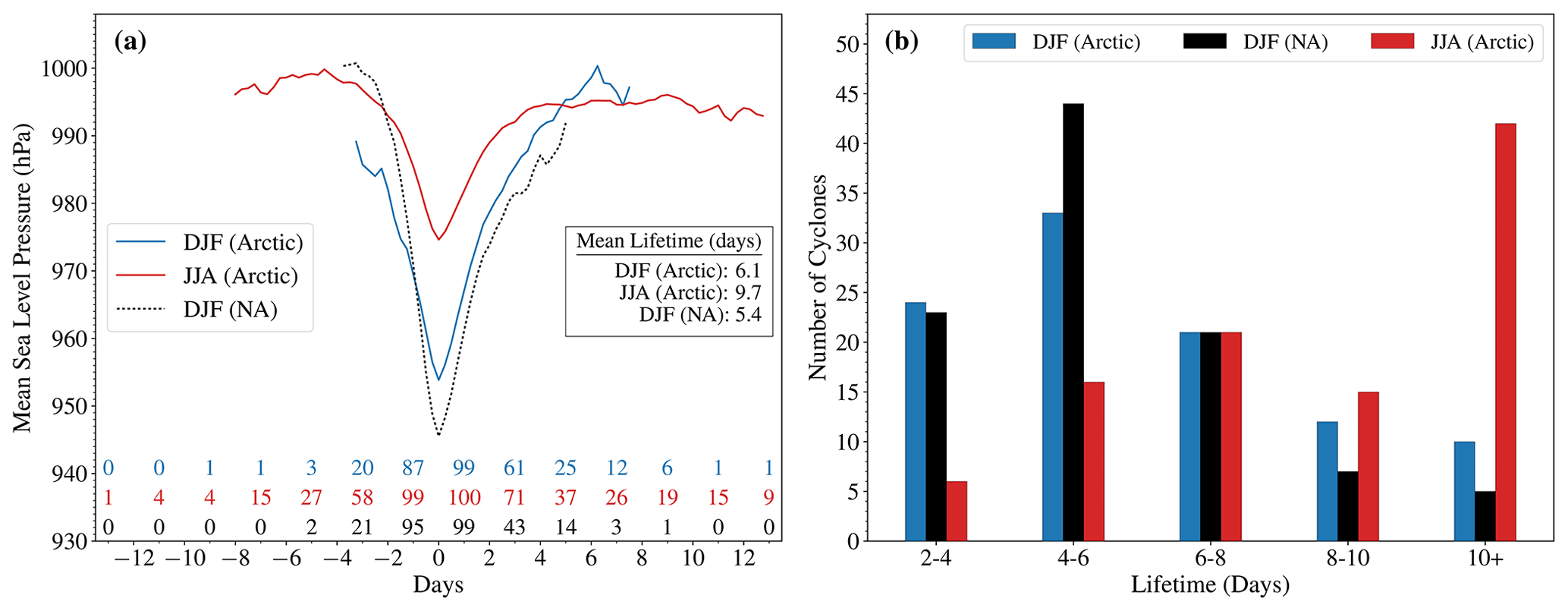
Figure 1 Lifecycles of the 100 most intense winter (DJF) and summer (JJA) Arctic cyclones and winter North Atlantic (NA) Ocean extra-tropical cyclones between 1979 and 2020. (a) The mean composite lifecycle development in intensity (minimum mean sea level pressure – MSLP) (hPa), when cyclones are centred at the time of their maximum intensity (i.e. minimum MSLP) and where at least 10 cyclones exist at each time interval. The numbers indicate how many cyclones exist at each time interval. (b) The distribution in the lifetimes of the 100 most intense winter and summer Arctic cyclones and winter North Atlantic (NA) Ocean extra-tropical cyclones.

The mean lifetime of the 100 most intense summer Arctic cyclones (9.7 d) is more than 3 d greater than that of the 100 most intense winter Arctic cyclones (6.1 d) and more than 4 d greater than that of the 100 most intense winter North Atlantic Ocean extra-tropical cyclones (5.4 d) (see Fig. 1a). This is also shown by more of the 100 most intense summer Arctic cyclones existing longer before and after their time of maximum intensity (see Fig. 1a). The modal lifetime of the 100 most intense summer Arctic cyclones is also greater than 10 d, with just under half of these cyclones (44) surpassing this threshold (see Fig. 1b). This is much greater than the modal lifetime of the 100 most intense winter Arctic and North Atlantic Ocean extra-tropical cyclones (4–6 d). With a longer lifetime, summer Arctic cyclones may cause prolonged hazardous weather conditions in the Arctic, such as extreme near-surface winds and high ocean waves (Thomson and Rogers, 2014; Liu et al., 2016; Waseda et al., 2018; Squire, 2020; Waseda et al., 2021).

3.2 Arctic cyclone spatial distribution

The track density of Arctic cyclones has been found in previous research to vary seasonally (Reed and Kunkel, 1960; Serreze et al., 2001; Simmonds et al., 2008; Crawford and Serreze, 2016; Vessey et al., 2020). Arctic cyclone track density is typically highest in winter over the Greenland, Norwegian, and Barents seas and over the Canadian Archipelago, whereas in summer, Arctic cyclone track density is typically highest over the coastline of Eurasia and the Arctic Ocean (Simmonds et al., 2008; Vessey et al., 2020). This is reflected in the spatial distribution of the locations of maximum intensity (i.e. minimum MSLP) of the 100 most intense winter and summer Arctic cyclones (see Fig. 2). Generally, the 100 most intense winter Arctic cyclones have their maximum intensity over the Greenland, Norwegian, and Barents seas (see Fig. 2). In contrast, the 100 most intense summer Arctic cyclones tend to have their maximum intensity over higher latitudes and over the Arctic Ocean that is north of the Eurasian coastline and the Bering Strait (see Fig. 2). This was similarly shown in Simmonds and Rudeva (2014).

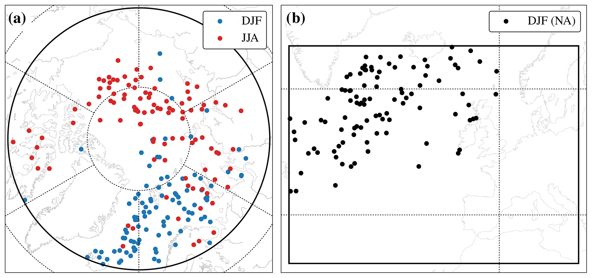
Figure 2 The locations of the points of maximum intensity (i.e. minimum MSLP) of each of the 100 most intense (a) winter (DJF) and summer (JJA) Arctic cyclones and (b) winter North Atlantic (NA) Ocean extra-tropical cyclones between 1979 and 2020. Longitudes are shown every 60^∘ E, and latitudes are shown at (a) 80, 65 (bold) and 60^∘ N, as well as at (b) 60 and 40^∘ N, with the thick black lines indicating the domains used for selecting each class of cyclone.

Over the past few decades, the Arctic has experienced the greatest change in mean surface temperature than any other region on Earth (Lenssen et al., 2019; GISTEMP Team, 2021). This raises the question of whether the occurrence of intense Arctic cyclones has changed over the last few decades. Figure S2 in the Supplement shows a time series by year of the occurrence of each cyclone within the sample of the 100 most intense cyclones per cyclone class. Overall, there is no visible trend in the frequency of intense winter North Atlantic Ocean extra-tropical cyclones (see Fig. S2a in the Supplement), winter Arctic cyclones (Fig. S2b in the Supplement), or summer Arctic cyclones (Fig. S2c in the Supplement).

3.3 Horizontal composite structure at the time of maximum intensity

The 100 most intense summer Arctic cyclones are less intense than winter Arctic cyclones and winter North Atlantic Ocean extra-tropical cyclones (see Fig. 1). Thus, the minimum MSLP of the summer Arctic cyclone composite at the time of maximum intensity (976.6 hPa) is higher than the winter Arctic cyclone (958.8 hPa) and North Atlantic Ocean extra-tropical cyclone (949.2 hPa) composites (see Fig. 3a, d, and g). The pressure gradients are tighter in the winter Arctic cyclone composite than in the summer Arctic cyclone composite but tightest in the winter North Atlantic Ocean extra-tropical cyclone composite.

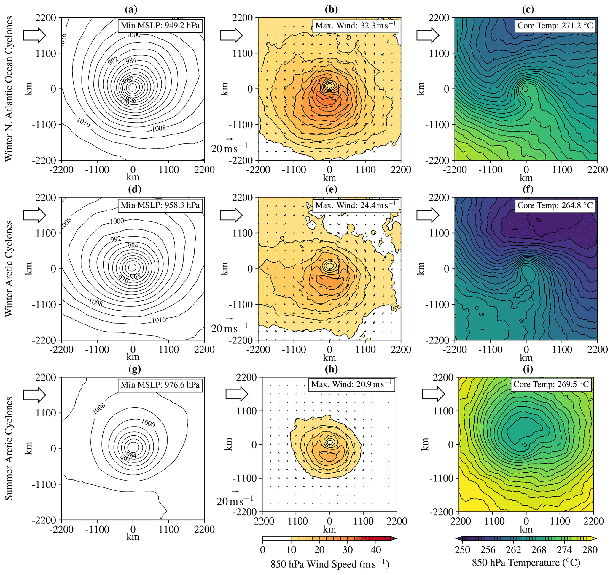
Figure 3 Horizontal mean sea level pressure (MSLP) (hPa) (a, d, g), 850 hPa earth-relative wind speed (m s⁻¹) (b, e, h), and 850 hPa temperature (^∘C) (c, f, i) composite structure at the time of maximum intensity (i.e. minimum MSLP) of winter (DJF) North Atlantic Ocean extra-tropical cyclones (a–c), winter Arctic cyclones (d–f), and summer (JJA) Arctic cyclones (g–i). The large arrow indicates the direction of cyclone propagation.

The summer Arctic cyclone composite also appears to be smaller in size than the winter Arctic and North Atlantic Ocean extra-tropical cyclone composites. This is inferred by the last closed isobar not exceeding the 2200 × 2200 km domain in the summer Arctic cyclone composite (see Fig. 3g). In contrast, the last closed isobar of the winter Arctic and North Atlantic Ocean cyclone composite does exceed the 2200 × 2200 km domain (see Fig. 3a and d). Moreover, the summer Arctic cyclone composite is more axi-symmetric than the winter Arctic and North Atlantic Ocean extra-tropical cyclone composites (see Fig. 3a, d, and g), which have tighter pressure gradients below the composite cyclone centre than above the composite cyclone centre.

The maximum 850 hPa earth-relative wind speeds are weaker in the summer Arctic cyclone composite (20.9 m s⁻¹) than the winter Arctic cyclone composite (24.5 m s⁻¹) and the winter North Atlantic Ocean extra-tropical cyclone composite (32.3 m s⁻¹) (see Fig. 3b, e, and h). These differences in magnitude between the cyclone composites in the 850 hPa earth-relative wind speeds, which would occur at an altitude of approximately 1 km above the surface, are also shown when analysing the composite 10 m earth-relative wind speeds per cyclone class (see Fig. S3 in the Supplement). Overall, the winter North Atlantic Ocean extra-tropical cyclone composite has the strongest 10 m wind speeds, and the summer Arctic cyclone composite has the weakest 10 m wind speeds. This is likely a consequence of the weaker pressure gradients within the summer Arctic cyclone composite.

In each cyclone composite, the maximum 850 hPa earth-relative wind speeds occur in the southern region of the composite and near the composite centre (see Fig. 3b, e, and h). Earth-relative winds are the combination of the cyclone's system-relative winds and the cyclone's propagation velocity. The cyclone composite 850 hPa earth-relative winds are highest in this region because the cyclonic (anti-clockwise) system-relative winds and the cyclone's propagation direction are in the same direction (see Fig. 3b, e, and h). Therefore the 850 hPa system-relative winds are enhanced by the propagation velocity, thus resulting in the highest 850 hPa earth-relative in the southern region of the cyclone composites. The area where the 850 hPa earth-relative wind speeds exceed 10 m s⁻¹ is also much greater in the winter Arctic and North Atlantic Ocean extra-tropical cyclone composites than the summer Arctic cyclone composite (see Fig. 3b, e, and h).

Despite similarities in the spatial distribution of the 850 hPa earth-relative winds within each composite, the 850 hPa temperature structure of the summer Arctic cyclone composite is different from that of the winter Arctic and North Atlantic Ocean extra-tropical cyclone composites (see Fig. 3c, f, and i). At the time of maximum intensity, the summer Arctic cyclone composite is characterized by a cold core at the centre of the composite (see Fig. 3i). In contrast, the winter Arctic and North Atlantic Ocean extra-tropical cyclone composites are characterized by high temperature gradients between the warm air below and cold air above the composite cyclone centres (see Fig. 3c and f). These divisions between warm and cold air would be associated with the location of weather fronts. The winter Arctic and North Atlantic Ocean extra-tropical cyclone composites also show signs that cold air has started to occlude into the warm air around the composite cyclone centre.

The 850 hPa temperature structure of the summer Arctic cyclone composite is different from the winter Arctic cyclone and winter North Atlantic Ocean extra-tropical cyclone composites. It is also different from that described in the Norwegian cyclone model and Shapiro–Keyser model (Bjerknes, 1919, 1922; Shapiro and Keyser, 1990). This contrasts with results from Clancy et al. (2022), who show that the structure of Arctic cyclones in every season is comparable to those in the mid-latitudes. However, Clancy et al. (2022) used a different cyclone compositing methodology, storm tracking algorithm that is applied to different reanalysis datasets (ERA-Interim and NCEP–NCAR reanalyses rather than ERA5), and metric of intensity to obtain the most intense cyclones. Clancy et al. (2022) also did not filter Arctic cyclones to retain the 100 most intense cyclones per season, instead calculating the cyclone composite as an average of thousands of cyclones per season, which may smooth out this unique axi-symmetric cold-core structure of the summer Arctic cyclone composite (see Fig. 3i).

3.4 Vertical composite structure at the time of maximum intensity

Cyclones typically contain conveyor belts, which are distinct airstreams occurring in different regions and altitudes within a cyclone (Browning, 1997; Catto et al., 2010; Dacre et al., 2012). These include a warm conveyor belt (WCB) that is typically located in front of the cold front and ascends from south to north parallel to the cold front. The WCB typically rises above the cold conveyor belt (CCB), which typically occurs at low levels in the atmosphere and wraps around above the cyclone centre (Browning, 1997).

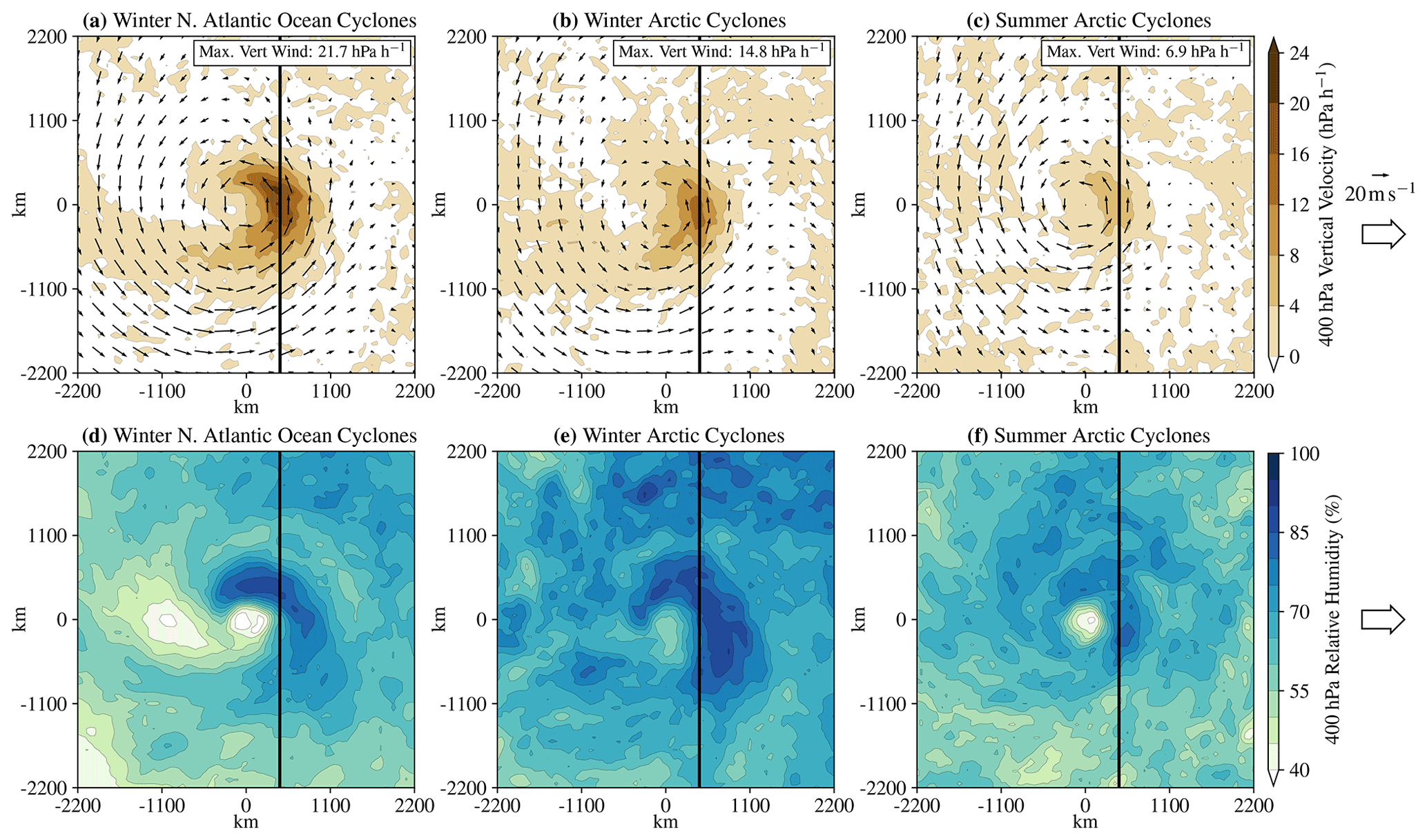
Figure 4 Horizontal 400 hPa system-relative winds (m s⁻¹) (quivers) and vertical velocity (hPa h⁻¹) (contours) (a–c) and 400 hPa relative humidity (%) (d–f) composite structure at the time of maximum intensity (i.e. minimum MSLP) of winter (DJF) North Atlantic Ocean extra-tropical cyclones (a, d), winter Arctic cyclones (b, e), and summer (JJA) Arctic cyclones (c, f). Positive values of vertical velocity indicate ascent. The large arrow indicates the direction of cyclone propagation. The transect (bold line) 4^∘ ahead of the composite cyclone centre and perpendicular to the cyclone's direction of propagation indicates the vertical slice used to produce Fig. 5.

The ascent of air associated with the WCB is shown in the winter North Atlantic Ocean extra-tropical cyclone and the winter Arctic cyclone composites ahead of the cyclone centre where the cold front would typically be located (see Fig. 4a, b, and c). This suggests that a WCB may be present within each composite. In the summer Arctic cyclone composite, the magnitude of ascent shown in the vertical velocity composite is much weaker than in the winter North Atlantic Ocean extra-tropical cyclone and Arctic cyclone composites (see Fig. 4). The maximum vertical velocity in the winter North Atlantic Ocean extra-tropical cyclone composite is 28.7 hPa h⁻¹, 17.2 hPa h⁻¹ in the winter Arctic cyclone composite, and 9.6 hPa h⁻¹ in the summer Arctic cyclone composite (see Fig. 4). This suggests that the WCB may be less well defined in summer Arctic cyclones.

The 400 hPa relative humidity composites for each class of cyclone show that the summer Arctic cyclone composite is more axi-symmetric than the winter North Atlantic Ocean extra-tropical cyclone composite and the winter Arctic cyclone composite (see Fig. 4d, e, and f). High values of relative humidity are more confined around the composite cyclone centre (above and to the right) in the winter North Atlantic Ocean extra-tropical cyclone and winter Arctic cyclone composites, perhaps indicating where moisture has risen from the surface within the cyclone at the typical location of weather fronts. To the left of the composite cyclone centre, drier air is shown at the 400 hPa level in the North Atlantic Ocean extra-tropical cyclone composite that appears to be intruding towards the composite cyclone centre, perhaps indicating the presence of a dry intrusion. But this feature is less pronounced in the winter and summer Arctic cyclone composites.

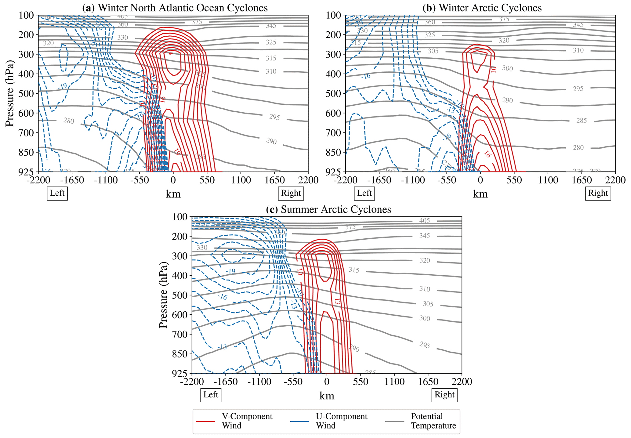
Figure 5 Composite vertical slices through the transect perpendicular to the direction of cyclone propagation and 4^∘ ahead of the composite cyclone centre (see Fig. 4) of (a) winter (DJF) North Atlantic Ocean extra-tropical cyclones, (b) winter Arctic cyclones, and (c) summer (JJA) Arctic cyclones. Red contours (shown every 1 m s⁻¹ from 10 m s⁻¹) show the V-component (meridional) winds, blue contours (shown every 1.0 m s⁻¹ below −10 m s⁻¹) show the U-component (zonal) winds, and grey contours (shown every 5 ^∘ up to 330 ^∘C and then every 15 ^∘C) show potential temperature isentropes. The positions (left/right) are shown relative to the cyclone propagation direction.

By analysing the transect outlined in Fig. 4, the CCB appears to be present in both the winter Arctic and North Atlantic Ocean cyclone composites (see Fig. 5a and b). The CCB is shown by the low-level high-magnitude system-relative zonal (U-component) wind speeds within the vertical cross section, which occur approximately 550 km from the composite cyclone centre. The magnitude of the zonal winds of the CCB is lower in the winter Arctic cyclone composite (approximately 18 m s⁻¹) than the winter North Atlantic Ocean cyclone composite (approximately 22 m s⁻¹). But in the summer Arctic cyclone composite, the highest zonal wind speeds above the cyclone composite centre do not occur at the surface (see Fig. 5c). Instead, the highest zonal wind speeds occur at the 300 hPa level approximately 1600 km from the cyclone composite centre. This suggests that the CCB, which typically occurs near the surface, is less well defined in summer Arctic cyclones.

The WCB is shown in the winter Arctic and North Atlantic Ocean cyclone composites by the high-magnitude meridional (V-component) system-relative winds within the vertical cross section, which occur south of the CCB and between 925 and 600 hPa (see Fig. 5a and b). Like the CCB, the maximum magnitude of these meridional wind speeds is lower in the winter Arctic cyclone composite (approximately 18 m s⁻¹) than the winter North Atlantic Ocean cyclone composite (approximately 20 m s⁻¹). The spatial distribution of the system-relative wind speeds in these composites is similar to that shown by Catto et al. (2010), who showed the composite structure of the 50 most intense North Atlantic and Pacific Ocean extra-tropical cyclones, using the ERA-40 reanalysis dataset. The stark changes in the wind direction shown above the cyclone composite centre in each cross section of the winter North Atlantic Ocean cyclone and Arctic cyclone composites indicate the presence of the CCB and WCB in each composite.

The distribution of the potential temperature isentropes within the summer Arctic cyclone composite cross section also differs from that of winter Arctic and North Atlantic Ocean extra-tropical cyclones (see Fig. 5). In contrast, the slope of the potential temperature isentropes reverses above the composite cyclone centre, where the isentropes ascend but then descend below and above the cyclone composite centre along this cross section (see Fig. 5c). At the time of maximum intensity, summer Arctic cyclones have developed a cold core (see Fig. 3), which could contribute to this distribution in the isentropes.

3.5 Development in the horizontal composite structure

The 700 hPa temperature structure of the winter North Atlantic Ocean extra-tropical cyclone composite and the winter and summer Arctic cyclone composites 48 h before the time of maximum intensity is similar, with each cyclone developing in a region of high temperature gradients (i.e. baroclinicity) (see Fig. 6). This is similar to the polar front described by Bjerknes (1919, 1922). Temperature gradients within the winter North Atlantic Ocean extra-tropical cyclone and Arctic cyclone composites are much greater than those of the summer Arctic cyclone composite. This is likely because intense winter Arctic cyclones also tend to develop over the North Atlantic Ocean (see Fig. 2), where meridional temperature gradients and baroclinicity are high, especially in winter (Serreze et al., 2001). However, from the time of maximum intensity, the development in the summer Arctic cyclone composite differs from that of the winter North Atlantic Ocean extra-tropical cyclone and Arctic cyclone composites.

Figure 6 Horizontal 700 hPa temperature anomaly (^∘C) composite structure 48 h before the time of maximum intensity (i.e. minimum MSLP) (a, d, g), at the time of maximum intensity (b, e, h), and 48 h after the time of maximum intensity (c, f, i) of winter (DJF) North Atlantic Ocean extra-tropical cyclones (a–c), winter Arctic cyclones (d–f), and summer (JJA) Arctic cyclones (g–i). The large arrow indicates the direction of cyclone propagation.

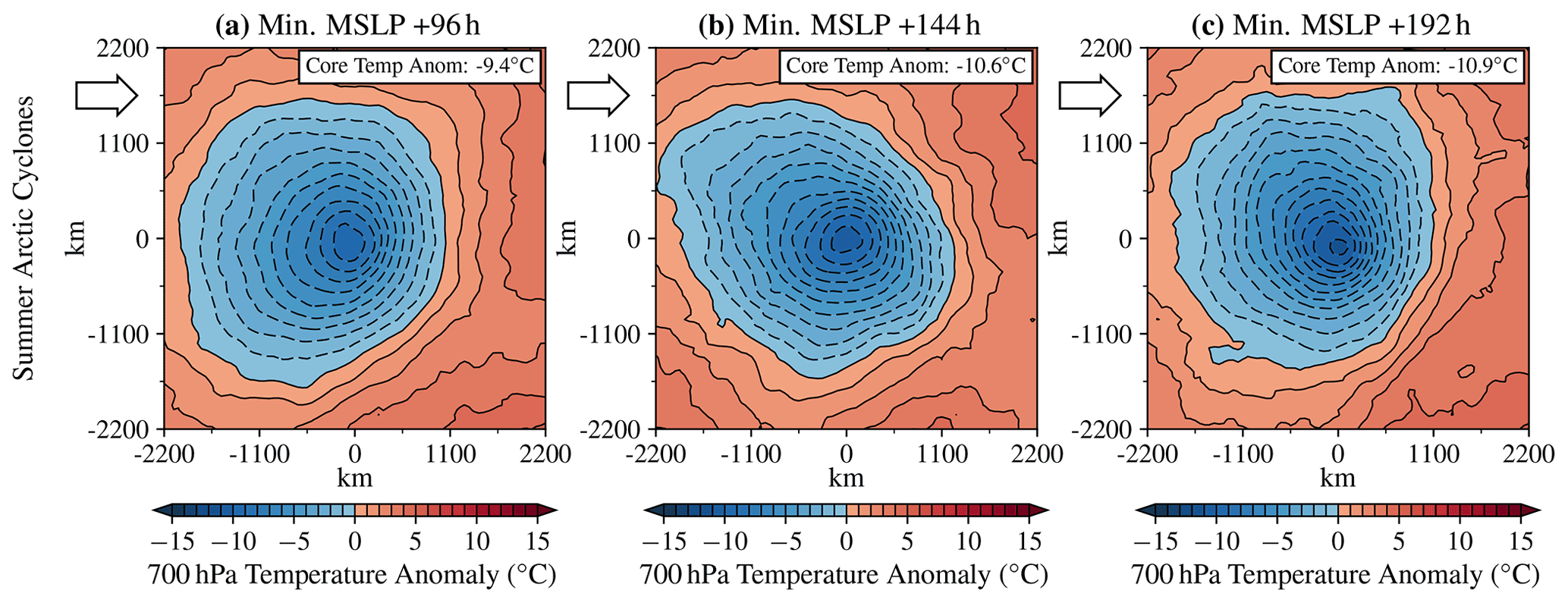
Figure 7 Horizontal 700 hPa temperature anomaly (^∘C) composite structure 96 h (a), 144 h (b), and 192 h (c) after the time of maximum intensity (i.e. minimum MSLP) of summer (JJA) Arctic cyclones. The large arrow indicates the direction of cyclone propagation.

After the time of maximum intensity, the summer Arctic cyclone composite develops a cold-core centre that becomes more defined and colder (see Figs. 6i and 7). The temperature anomaly at the composite cyclone centre at the time of maximum intensity is −3.8 ^∘C (see Fig. 6h) but lowers to −8.7 and −10.6 ^∘C at 48 and 144 h after the time of maximum intensity (see Figs. 6i and 7b). This suggests that summer Arctic cyclones tend to develop a cold-core centre around the time of maximum intensity and retain this structure until they dissipate.

This is in contrast with the winter Arctic and North Atlantic Ocean extra-tropical cyclone composites that appear to follow the process of occlusion, in which cold air wraps around the composite centre (see Fig. 6). This structural transition of the summer Arctic cyclone composite is also different from the Norwegian cyclone model (Bjerknes, 1919, 1922), in which cyclones tend to undergo occlusion, and the Shapiro–Keyser model (Shapiro and Keyser, 1990), in which cyclones tend to undergo frontal fracture and develop a warm core centre.

3.6 Development in the vertical composite structure

The unique structural transition in temperature of the summer Arctic cyclone composite is also shown throughout the vertical extent of the composite, from the surface up to the 100 hPa level (see Fig. 8). From the time of maximum intensity, cold air in the summer Arctic cyclone composite appears to intrude through the centre of the composite, which ultimately leads to the composite developing a cold-core structure throughout the troposphere (see Fig. 8g, h, and i). This is a similar structural development to the “The Great Arctic Cyclone of 2012”, which was shown by Aizawa and Tanaka (2016).

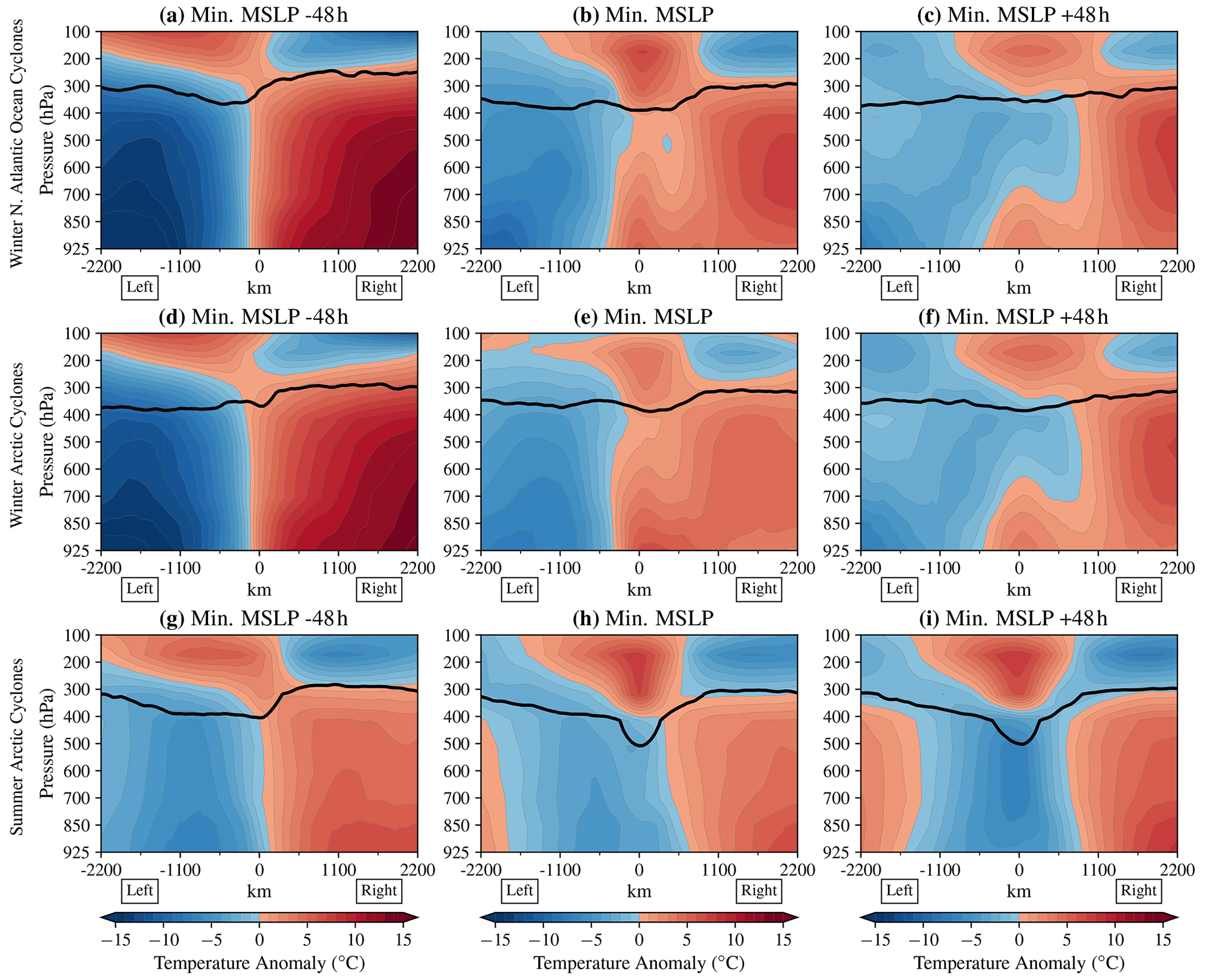
Figure 8 Vertical temperature anomaly (^∘C) composite of winter (DJF) North Atlantic Ocean extra-tropical cyclones (a–c), winter Arctic cyclones (d–f), and summer (JJA) Arctic cyclones (g–i) along the transect perpendicular to the cyclone propagation direction through the composite cyclone centre 48 h before the time of maximum intensity (i.e. minimum MSLP) (a, d, g), at the time of maximum intensity (b, e, h), and 48 h after the time of maximum intensity (c, f, i). The thick black contour indicates the level of the tropopause (i.e. the 2 PVU, potential vorticity units, contour). The positions (left/right) are shown relative to the cyclone propagation direction.

The temperature anomaly in the stratosphere is also much more defined and larger (between 8.0 and 9.0 ^∘C) in the summer Arctic cyclone composite at and after the time of maximum intensity (see Fig. 8h and i). In contrast, the maximum temperature anomaly in the stratosphere after the time of maximum intensity in the winter North Atlantic Ocean extra-tropical cyclone and Arctic cyclone composites is between 5.0 and 6.0 ^∘C (see Fig. 8). Furthermore, the altitude of the tropopause is much lower in the summer Arctic cyclone composite at and after the time of maximum intensity than the winter North Atlantic Ocean extra-tropical cyclone and Arctic cyclone composites (see Fig. 8). The level of tropopause is shown to be approximately 500 hPa at the centre of the summer Arctic cyclone composite at and after the time of maximum intensity. In contrast, the level of tropopause is approximately 300 hPa at the centre of the winter North Atlantic Ocean extra-tropical cyclone and Arctic cyclone composites at and after the time of maximum intensity. These differences suggest that the development of intense summer Arctic cyclones may be more influenced by the stratosphere than intense winter Arctic and North Atlantic Ocean extra-tropical cyclones.

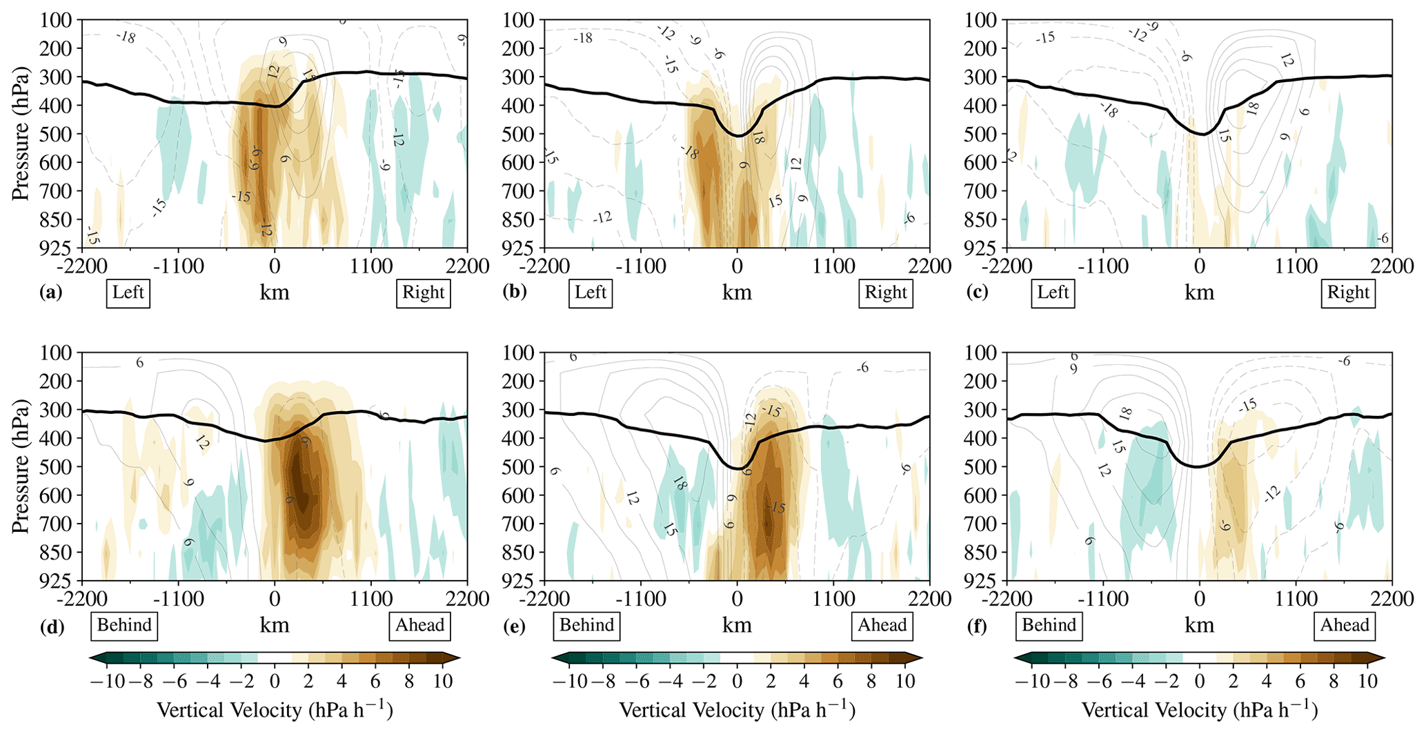
Figure 9 Vertical velocity (hPa h⁻¹) (colour) and system-relative (m s⁻¹) U-component (zonal) and V-component (meridional) wind speed (contours) composite structure of the 100 most intense summer (JJA) Arctic cyclones along the transect perpendicular to the cyclone propagation direction through the composite cyclone centre (a–c) and along the transect parallel to the cyclone propagation direction through the composite cyclone centre (d–f). Positive values of vertical velocity indicate ascent. Composites are shown 48 h before the time of maximum intensity (i.e. minimum MSLP) (a, d), at the time of maximum intensity (b–e), and 48 h after the time of maximum intensity (c–f). The thick black contour indicates the level of the tropopause (i.e. the 2 PVU contour).

The vertical temperature structure of the summer Arctic cyclone composite is shown to be more axi-symmetric from the time of maximum intensity than the winter North Atlantic Ocean cyclone and winter Arctic cyclone composites (see Fig. 8). This axi-symmetric structure after the time of maximum intensity is also shown in the system-relative wind speed fields (see Fig. 9). After 48 h from the time of maximum intensity, the summer Arctic cyclone composite develops high system zonal and meridional system-relative winds around the composite cyclone centre, with a similar magnitude each side of the composite cyclone (see Fig. 9c and f). Notably, system-relative winds are lower near the surface than in the upper atmosphere, where human activity would tend to occur.

3.7 Comparison of the summer Arctic cyclone composite to the Aizawa and Tanaka (2016) model

Aizawa and Tanaka (2016) proposed a conceptual model describing the structure of summer Arctic cyclones based on just two past summer Arctic cyclone case studies. Here, the composite structure of the 100 most intense summer Arctic cyclones has been determined, allowing for an evaluation of the Aizawa and Tanaka (2016) conceptual model with the composite structure of a greater sample of past intense summer Arctic cyclones. This conceptual model highlights six main features of summer Arctic cyclones, which include a warm core in the lower stratosphere and cold core in the troposphere, a deep tropopause fold descending down to 500 hPa over the cyclone centre, a secondary circulation in the troposphere, a downdraught in the lower stratosphere, and a deep cyclonic circulation up into the stratosphere. Aizawa and Tanaka (2016) also describe summer Arctic cyclones as being one of the largest cyclone types found on the Earth, with a horizontal diameter of 5000 km at upper levels (i.e. in the stratosphere).

There are similarities between the summer Arctic cyclone composite and this conceptual model. The composite vertical structure of summer Arctic cyclones shows a warm anomaly in the lower stratosphere (above the tropopause) and a cold core throughout the troposphere (see Fig. 8). There is also a deep tropopause fold that descends to 500 hPa shown in the summer Arctic cyclone composite (see Fig. 8).

Despite these similarities, the summer Arctic cyclone composites do also show differences from the Aizawa and Tanaka (2016) model. The general size of the summer Arctic cyclone composite appears to be smaller near the surface than the winter Arctic and North Atlantic Ocean cyclone composites (see Fig. 3). This is implied by the area within the last-closed isobar (see Fig. 3a, d, and g), as well as the area within the 10 m s⁻¹ earth-relative wind speed contour of each cyclone composite (see Fig. 3b, e, and h). Although Aizawa and Tanaka (2016) use a different metric to infer cyclone size, the summer Arctic cyclone composite is smaller in size than the winter Arctic and North Atlantic Ocean cyclone composites near the surface.

The summer Arctic cyclone composite from the time of maximum intensity also does not show a secondary circulation in the troposphere, a deep cyclonic circulation into the stratosphere, or a downdraught in the stratosphere (Fig. 9). Before and after the time of maximum intensity, the summer Arctic cyclone composite does not show downdraughts (negative vertical velocity) on the outer flanks or in the centre of the composite (see Fig. 9). Only weak (> −3.0 hPa h⁻¹) downdraughts are shown in the composite before and at the time of maximum intensity (see Fig. 9).

Overall, by analysing the composite structure of a larger sample of past summer Arctic cyclones, there is evidence to support some aspects of the Aizawa and Tanaka (2016) conceptual model. Results from this study show that after the time of maximum intensity, intense summer Arctic cyclones do indeed likely have a warm core in the lower stratosphere and a cold core throughout the troposphere, as well as a deep tropopause fold descending into the troposphere over the cyclone centre. However, there is insufficient evidence in this study to suggest that intense summer Arctic cyclones typically have a secondary circulation in the troposphere, a downdraught in the lower stratosphere, a deep cyclonic circulation up into the stratosphere, and a horizontal extent of approximately 5000 km (typical summer Arctic cyclones are likely smaller).

An aspect that is highlighted in this study is that intense summer Arctic cyclones appear to typically undergo a structural transition during their lifecycle. The development in the composite structure of intense summer Arctic cyclones shows that they undergo a transition from having a baroclinic structure to an axi-symmetric cold-core structure throughout the troposphere around the time of maximum intensity. After this transition, the structure of intense summer Arctic cyclones is somewhat similar to the Aizawa and Tanaka (2016) model, though without the differences from this model described above. Aizawa and Tanaka (2016) showed this structural transition when analysing “The Great Arctic Cyclone of 2012” and for another summer Arctic cyclone in June 2008. The composite summer Arctic cyclone shown in this study suggests that this transition has likely occurred in other past intense summer Arctic cyclones and that it may be typical of intense summer Arctic cyclones.

4 Summary and conclusions

The location and intensity of hazardous weather within a cyclone is dependent on its development and structure. Previous analysis of individual past summer Arctic cyclones suggests that they may have a different structure from typical extra-tropical cyclones (e.g. Tanaka et al., 2012; Aizawa et al., 2014; Aizawa and Tanaka, 2016; Tao et al., 2017). However, these previous studies only focused on individual case studies; therefore the generality in the development and structure of Arctic cyclones has not yet been determined.

This study aims to describe the typical lifetime, structure, and development of a large sample of past intense Arctic cyclones using a storm compositing methodology. The composite structure of the 100 most intense summer (JJA) and winter (DJF) Arctic cyclones is compared with that of the 100 most intense winter extra-tropical cyclones occurring over the North Atlantic Ocean between 1979 and 2020 using data from the ERA5 reanalysis dataset. Overall, this study shows that summer Arctic cyclones are typically longer lived and have a different development in their composite structure from winter Arctic and North Atlantic Ocean extra-tropical cyclones and from that described in conceptual models such as the Norwegian cyclone model (Bjerknes, 1919, 1922) and the Shapiro–Keyser model (Shapiro and Keyser, 1990).

• Intense summer Arctic cyclones have longer lifetimes than winter Arctic cyclones and North Atlantic Ocean extra-tropical cyclones.

Cyclones are associated with hazardous weather, including high wind speeds and high ocean waves (Thomson and Rogers, 2014; Liu et al., 2016; Waseda et al., 2018; Squire, 2020; Waseda et al., 2021). Arctic cyclones can also enhance the break-up of sea ice, which may then become mobile and drift toward shipping lanes, creating an additional hazard to shipping, oil exploration, and tourism activities (Simmonds and Keay, 2009; Screen et al., 2011; Asplin et al., 2012; Parkinson and Comiso, 2013; Peng et al., 2021). It is found that summer Arctic cyclones are typically much longer lived than winter Arctic and North Atlantic Ocean extra-tropical cyclones. The mean lifetime of the 100 most intense summer Arctic cyclones is found to be more than 3 d longer than that of the 100 most intense winter Arctic and North Atlantic Ocean extra-tropical cyclones. Consequently, summer Arctic cyclones may cause prolonged hazardous and disruptive weather conditions to human activities in the Arctic.

• The development shown in the composite structure of intense summer Arctic cyclones is different from that of winter Arctic and North Atlantic Ocean extra-tropical cyclones and from the description given in conceptual models such as the Norwegian cyclone model (Bjerknes, 1919, 1922) and Shapiro–Keyser model (Shapiro and Keyser, 1990).

The development shown in the composite structure of the 100 most intense summer Arctic cyclones shows that they typically undergo a transition from having a baroclinic structure to having an axi-symmetric cold-core structure throughout the troposphere around the time of maximum intensity (i.e. the time of minimum mean sea level pressure). This axi-symmetric cold-core structure is consistent with previous studies that have analysed past individual summer Arctic cyclone case studies (Tanaka et al., 2012; Aizawa et al., 2014; Aizawa and Tanaka, 2016; Tao et al., 2017). In comparison, the composite structure of the 100 most intense winter Arctic cyclones is similar to that of the 100 most intense North Atlantic Ocean extra-tropical cyclones, with both of the cyclone composites showing a baroclinic structure with high meridional temperature gradients and signs of occlusion throughout their lifecycle. From the time of maximum intensity, the summer Arctic cyclone composite has a much lower-lying tropopause and a larger positive temperature anomaly in the stratosphere at the centre of the cyclone composite than the winter Arctic and North Atlantic Ocean extra-tropical cyclone composites. The summer Arctic cyclone composite retains this axi-symmetric cold-core structure long after the time of maximum intensity.

The composite structural development of summer Arctic cyclones is found to be different from that of winter North Atlantic Ocean extra-tropical cyclones and winter Arctic cyclones. This is also different from the structural development of extra-tropical cyclones described in the Norwegian cyclone model (Bjerknes, 1919, 1922) and Shapiro–Keyser model (Shapiro and Keyser, 1990). The summer Arctic cyclone composite also shows differences from the Arctic cyclone model proposed by Aizawa and Tanaka (2016). This raises questions such as whether this unique structural transition of summer Arctic cyclones is captured in climate model projections and weather forecasting models, and how the frequency of these summer Arctic cyclones might change in response to climate change.

The results found in this study contrast with those in Clancy et al. (2022), who show that the structure of Arctic cyclones in all seasons is similar to mid-latitude cyclones. However, there are numerous differences in the methods between this study and Clancy et al. (2022). In this study, cyclone composites were calculated across the 100 most intense cyclones per season, but in Clancy et al. (2022), thousands more cyclones were included when producing cyclone composites. It is possible that this unique structural development of summer Arctic cyclones is only present in the most intense summer Arctic cyclones and explains why it was shown in this study and not in Clancy et al. (2022). In addition, Clancy et al. (2022) use a different cyclone compositing method, different storm tracking algorithm applied to different reanalysis datasets, and a different intensity metric to determine the most intense cyclones that contribute to their composites. These differences in method may also contribute to the differences in the results presented in this study. Future work may seek to test the sensitivity of sample size and composite method on determining the structure of intense Arctic cyclones.

It is plausible that the structural transition of summer Arctic cyclones, which do not fully undergo occlusion, may contribute to extending the lifetimes of such cyclones. Summer Arctic cyclones may lack the dynamical forcing from the occlusion process that typically helps to force the movement of air that leads to the dissipation of extra-tropical cyclones. The summer Arctic cyclone composite is also found to have a lower tropopause and greater temperature anomaly in the stratosphere at the composite centre than the winter Arctic and North Atlantic Ocean extra-tropical cyclone composites. This suggests that they may be more strongly influenced by the stratosphere and, in particular, tropopause polar vortices (TPVs) that are common features based on the tropopause in the Arctic (Cavallo and Hakim, 2010). Recent studies have suggested that some Arctic cyclones may have been strongly influenced by TPVs (e.g. Simmonds and Rudeva, 2014; Tao et al., 2017; Gray et al., 2021). Understanding what causes this structural transition of summer Arctic cyclones and why they tend to have longer lifetimes than winter Arctic and extra-tropical cyclones is an area for future research.