The impact of microphysical uncertainty conditional on initial and boundary condition uncertainty under varying synoptic control

The relative impact of individual and combined uncertainties of cloud condensation nuclei (CCN) concentration and the shape parameter of the cloud droplet size distribution (CDSD) in the presence of initial and boundary condition uncertainty (IBC) on convection forecasts is quantified using the convection-permitting model ICON-D2 (ICOsahedral Non-hydrostatic). We performed 180-member ensemble simulations for five real case studies representing different synoptic forcing situations over Germany and inspected the precipitation variability on different spatial and temporal scales. During weak synoptic control, the relative impact of combined microphysical uncertainty on daily area-averaged precipitation accounts for about one-third of the variability caused by operational IBC uncertainty. The effect of combined microphysical perturbations exceeds the impact of individual CCN or CDSD perturbations and is twice as large during weak control. The combination of IBC and microphysical uncertainty affects the extremes of daily spatially averaged rainfall of individual members by extending the tails of the forecast distribution by 5 % in weakly forced conditions. The responses are relatively insensitive in strong forcing situations. Visual inspection and objective analysis of the spatial variability in hourly rainfall rates reveal that IBC and microphysical uncertainties alter the spatial variability in precipitation forecasts differently. Microphysical perturbations slightly shift convective cells but affect precipitation intensities, while IBC perturbations scramble the location of convection during weak control. Cloud and rainwater contents are more sensitive to microphysical uncertainty than precipitation and less dependent on synoptic control.

1 Introduction

Weather forecasts are subject to many sources of uncertainty. The uncertainties originate from, among others, the unknown true state of the atmosphere, as well as imperfect representations and approximations of physical processes in numerical weather prediction (NWP) models. The chaotic nature of the atmosphere can amplify inherent uncertainties leading to reduced forecast accuracy and limited predictability.

Ensemble prediction systems (EPSs) allow us to estimate the forecast uncertainty. In regional convective-scale EPSs, there are essentially three key sources of uncertainty. First, initial condition uncertainty is usually implemented by means of variational or ensemble data assimilation systems (Bannister, 2017; Schraff et al., 2016). Secondly, lateral boundary condition uncertainty necessary to avoid underdispersion of the ensemble is mostly provided by coarser ensemble forecasts at regular time intervals throughout the forecast horizon. Thirdly, there is an incomplete description of physical processes and an insufficient representation of the subgrid-scale variability in NWP models also known as model error.

One of the crucial benefits of convective-scale models is the possibility to explicitly describe (deep) moist convection and thus to be able to omit an error-prone parametrisation scheme for deep convection that is a known model error source. Other important physical processes that are not resolved in models with kilometre-scale grid spacings and need to be accurately represented to forecast convective precipitation comprise boundary-layer turbulence, cloud microphysics and its interaction with aerosols (Clark et al., 2016). In the present study, we inspect the relative impact of a cloud microphysical uncertainty in combination with different aerosol concentrations both implemented in a full convective-scale EPS framework including initial and lateral boundary condition (IBC) uncertainty.

Microphysical processes are essential to forming precipitation. Due to their inherent small spatial and temporal scale these processes are not only difficult to observe but also to understand and represent in NWP models. Moreover, many microphysical processes are insufficiently constrained by observations. The impact of parameter perturbations in microphysics parametrisations has been studied extensively with mostly single deterministic idealised (e.g. Grant and van den Heever, 2015; Glassmeier and Lohmann, 2018; Heikenfeld et al., 2019; Chua and Ming, 2020; Wellmann et al., 2020) or realistic (e.g. Bryan and Morrison, 2012; Barthlott and Hoose, 2018; Schneider et al., 2019; Baur et al., 2022; Barthlott et al., 2022a, b) simulations using a variety of NWP models and schemes. However, because of the large variability between schemes and cases, results from different systems are difficult to generalise.

The impact of aerosols on microphysical processes in the formation of convective clouds and precipitation remains highly uncertain. The amount of aerosol in the atmosphere is one of the important factors influencing cloud formation. In general, more aerosol particles, which act as cloud condensation nuclei (CCN), activate condensation and increase the cloud water content while reducing the average size of cloud droplets. Smaller cloud droplet sizes and more narrow cloud droplet size distributions (CDSDs) inhibit the generation and growth of raindrops primarily caused by the collision–coalescence process, thus prolonging the lifetime of clouds (Albrecht, 1989). A smaller droplet size shows a negative impact on precipitation in many cases, but the impact of CCN perturbations on precipitation is not always straightforward, as an increase in CCN provides more cloud water. Systematic responses of varied CCN concentrations on precipitation are reported in numerous studies with a large variety depending on the model used and case chosen (Table 1 in Tao and Li, 2016). For example, Fan et al. (2009) show a negative impact and the dependence of wind conditions in idealised large-eddy simulations using a bin microphysics scheme, while Wang (2005) and Baur et al. (2022) show positive ones attributed to convection enhancement and the suppression of rain evaporation, respectively, using two-moment bulk microphysics schemes with a grid spacing of around 2 km. Keil et al. (2019) evaluate the impact of CCN uncertainties on precipitation and find that the spread of CCN-perturbed ensemble forecasts is greater than the impact due to soil moisture. This effect is more pronounced during atmospheric conditions when the synoptic-scale forcing is weak.

In current operational NWP systems, grid-scale microphysical processes are mostly approximated by cost-efficient one-moment bulk microphysics schemes due to the limitation of computational resources. In these parametrisations only the hydrometeor mass is prognostic. In two-moment microphysics schemes that are widely used in research, the number concentration of hydrometeors can also be predicted. It is therefore possible to calculate mean particle radii at each model grid point and estimate more realistic CDSDs. The shape of the CDSD is controlled by ν, the pre-defined shape parameter.

The width of the CDSD is not well constrained by observations, and previous observational studies revealed a large range of the shape parameter between 0–14 (see, for example, Table 1 in Igel and van den Heever, 2017b). Thus the shape of the CDSD constitutes a potentially relevant source of microphysical uncertainty to be included in ensemble systems.

In general, the broader the CDSD is, the more efficient the collision–coalescence process will be, since hydrometeor particles of various sizes are present in the atmosphere. Hence the shape parameter perturbation of the CDSD affects the cloud lifetime and raindrop growth as well. The importance of the CDSD on precipitation forecasts has been evaluated by means of idealised simulations (e.g. Igel and van den Heever, 2017a). Recently, Barthlott et al. (2022a, b) showed that narrowing of the CDSD can produce almost as large a variation in precipitation as a CCN increase from maritime to polluted conditions in realistic simulations.

The ultimate impact of various uncertainties described above varies greatly depending on the prevailing flow conditions. A successful approach to classify convective precipitation regimes is to focus on the strength and type of forcing that is driving convection. An objective measure for such a classification constitutes the convective adjustment timescale τ_c that provides a timescale over which CAPE (convective available potential energy) is consumed by precipitation. In strong synoptic forcing situations, when ascending motions caused by the synoptic-scale flow lead to precipitation and the continuously produced CAPE is consumed immediately, the regime is in a kind of equilibrium, in which τ_c attains small values. On the other hand, in a weak synoptic forcing situation, CAPE accumulates until local phenomena that can initiate convection occur and precipitation shows an intermittent character. In this situation, τ_c can temporarily increase, especially before the initiation of convective precipitation in the afternoon. The strength of the synoptic control is found to influence the predictability and the impact of different types of perturbations on precipitation (Flack et al., 2016, 2018; Keil et al., 2019; Weyn and Durran, 2019).

The goal of the present study is to estimate the relative importance of microphysical uncertainties of precipitation in the presence of IBC uncertainties conditional on different synoptic control across central Europe. The microphysical perturbations comprise three different aerosol concentrations and three different shape parameters governing the CDSD. We conduct 180-member ensemble experiments using an operational convective-scale NWP system for 5 d in August 2020 during different weather conditions. Specifically, the following research questions are addressed in this study:

• What is the relative impact of individual and combined microphysical uncertainties on convective precipitation forecasts at different spatial and temporal scales?

• How dependent on the weather regime is that impact?

• What is the impact on convective clouds and does the impact on cloud content translate into a comparable impact on precipitation?

In the remainder of the paper, we present the numerical model and the experimental design that allow for the examination of the relative impact based on different sub-sampling approaches (Sect. 2). Following the description and classification of the weather situations in Sect. 3 we present results of precipitation forecasts and different spatio-temporal scales in the next section. This is complemented by a brief discussion about the relative impact on cloud and rainwater contents. Before concluding with a summary in Sect. 5 we present aggregated results encompassing five cases.

2 Model and experimental design

2.1 Model description

The numerical simulations are performed with the ICON (ICOsahedral Non-hydrostatic, version 2.6.2.2) model in its limited-area mode ICON-D2 covering central Europe (see Fig. 2). The ICON-D2-EPS has been the operational ensemble NWP system at Deutscher Wetterdienst (DWD) since February 2021 (Reinert et al., 2021). We use an almost equivalent configuration with a few exceptions described below. ICON-D2 employs an icosahedral-triangular Arakawa-C grid with a grid spacing of 2 km (542 040 grid points) and 65 vertically discretised layers from the ground to 22 km above mean sea level. Its dynamical core is based on the non-hydrostatic equations for fully compressible fluids as governing equations (see Zängl et al., 2015, for the details). Different from the operational configuration, the two-moment bulk microphysics scheme (Seifert and Beheng, 2006) is used to be able to investigate the impact of number densities and the size distributions of cloud water droplets (by perturbing the CCN concentration and shape of the CDSD, respectively, as in Barthlott et al., 2022a, b). Note that the operationally used parameter perturbations in ICON-D2-EPS are turned off here to purely focus on the impact of microphysical perturbations that exclusively represent the model error in the present study.

2.2 Experimental design

To investigate the influence of uncertainties on CCN concentration and the shape of the CDSD in the presence of characteristic IBC uncertainty, we perform numerical experiments using 20 different IBCs, 3 different CCN concentrations and 3 different shape parameters of the CDSD yielding in total a 180-member ICON-D2 ensemble (Fig. 1a).

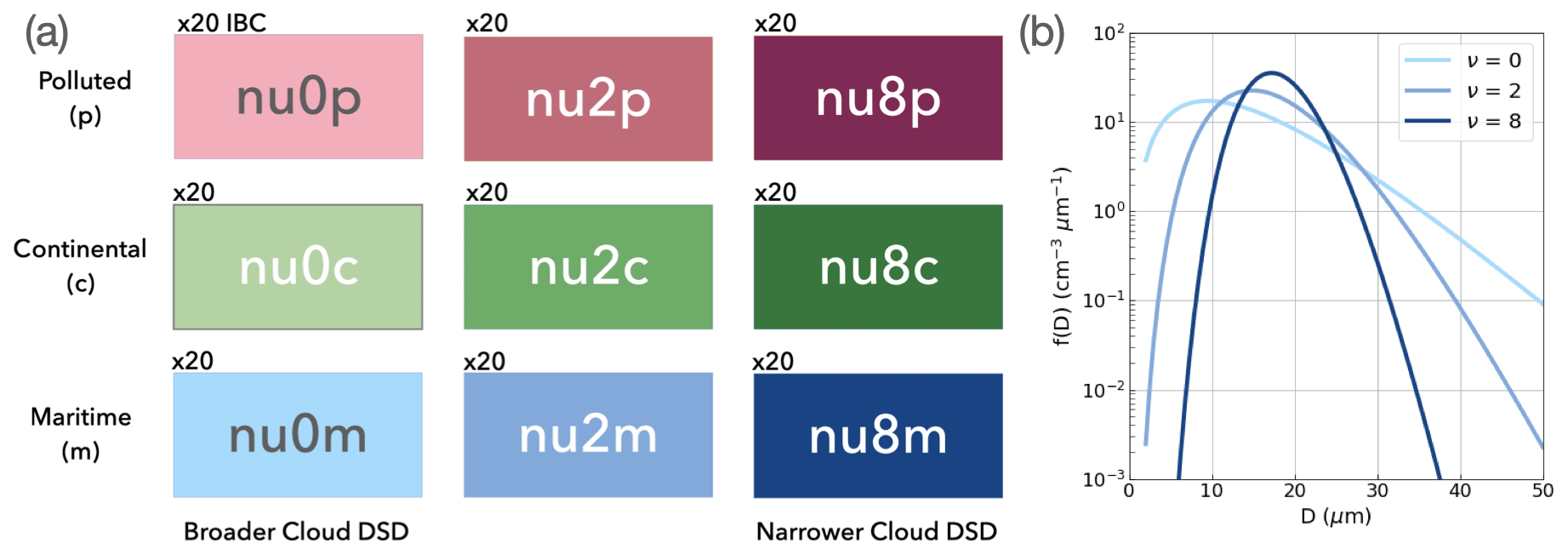
Figure 1 (a) Design of microphysically perturbed ensemble experiments. The colours used throughout the article indicate the nine different 20-member IBC sub-ensembles sharing the same combination of CCN and CDSD parameters. (b) Cloud droplet size distribution with different shape parameter ν at fixed cloud water content (QC = 1 g m⁻³) and cloud droplet number concentration (QNC = 300 cm⁻³). D denotes the diameter of the droplets.

The initial conditions are provided by pre-operational analyses produced by ICON-D2-KENDA (Kilometer-scale ENsemble Data Assimilation (Schraff et al., 2016)). In August 2020 conventional measurements like radiosonde, aircraft and ground-based observations were assimilated in ICON-D2-KENDA using the local ensemble transform Kalman filter (LETKF; Hunt et al., 2007). ICON-D2-KENDA produces 40-member ensemble analyses, while the first 20 analyses are used as initial conditions for ICON-D2 ensemble forecasts (as in operations at DWD) with 24 h lead time due to limited computational resources. Lateral boundary conditions are based on ensemble ICON global and EU-nest simulations initialised 3 h before the initial time of the ICON-D2 ensemble experiments. The initial conditions for the global and EU-nest simulations are the operational analyses provided by DWD with a grid spacing of 40 km for the global domain and 20 km for the nested EU domain. Different from our ICON-D2 ensemble simulations the one-moment microphysics scheme and the convection parametrisation for deep and mid-level convection are active in the ICON global and EU-nest simulations. The lateral boundary conditions are updated hourly using data from the EU-nest forecasts at lead times from 3 to 27 h.

To examine the microphysical uncertainty we perturb the width of the CDSD and the amount of aerosol in the atmosphere by altering the CCN concentration. In the Seifert and Beheng (2006) scheme, CCN activation rates are calculated using a look-up table of activation rates empirically estimated by Segal and Khain (2006). To take insoluble CCN into account, certain portions of CCN are not activated depending on their particle sizes (Seifert et al., 2012). Consistent with Barthlott et al. (2022a, b) we vary CCN concentrations between pristine conditions and extremely polluted conditions. We employ three CCN concentrations: maritime (N_CN = 100 cm⁻³), continental (N_CN = 1700 cm⁻³) and polluted (N_CN = 3200 cm⁻³). The “maritime” emulates clean, pristine conditions that have quite small numbers of CCN like over the sea. The “continental” is the default setting that mimics the observed CCN concentrations for the European continental regions (Hande et al., 2016). The “polluted” represents extremely polluted situations caused by, for example, massive wildfires and considerable anthropogenic emissions. The different CCN sub-ensembles that share the same CCN concentration are named with suffixes m(aritime), c(ontinental) and p(olluted), as shown in Fig. 1a.

The size distribution of hydrometeors is approximated using the following generalised gamma distribution:

$$\begin{array}{}\text{(1)}& f\left(x\right)=A{x}^{\mathit{\nu }}\exp \left(-\mathit{\lambda }{x}^{\mathit{\mu }}\right),\end{array}$$

where A is dependent on the number density of hydrometeor particles, and λ is a coefficient dependent on the average particle mass. The coefficients ν and μ are parameters that are pre-defined and fixed throughout a simulation. For example, with $\mathit{\mu }=\frac{\mathrm{1}}{\mathrm{3}}$ and $\mathit{\nu }=-\frac{\mathrm{2}}{\mathrm{3}}$, we can obtain the so-called Marshall–Palmer distribution of raindrops. In this study we control the widths of the particle size distributions by varying the shape parameter ν (for details see Barthlott et al., 2022a, b). With increasing ν the CDSD becomes narrower and more skewed as shown in Fig. 1b, which means the number concentrations of particles close to the mean size increase. In this study ν is varied between 0, 2 and 8 to cover a wide spectrum of the possible shape parameter values (as in Wellmann et al., 2020; Barthlott et al., 2022a, b). Note that the default setting is the broadest CDSD ν=0. Since the parameters describing the CCN concentration and the shape of the CDSD are kept temporally and spatially constant throughout the simulation, they rather represent model error due to the incomplete description of physical processes than subgrid-scale variability.

To address individual or combined impacts of forecast uncertainties mentioned above, we employ a sub-ensemble approach. A simple selection of different sub-ensembles sharing the same uncertainty allows us to quantify the relative impact of the various uncertainties. To focus on the combined impact of the microphysical perturbations, for instance, we can inspect 20 microphysical sub-ensembles consisting of nine members each sharing the same IBC but different combinations of CCN and CDSD parameters (microphysical (MP) sub-ensemble). To focus on the impact of the IBC uncertainties, we have nine IBC sub-ensembles available consisting of 20 members each (IBC sub-ensemble).

3 Weather situation and classification of cases

Two typical cases are selected for an in-depth investigation of the relative importance of the different uncertainties conditional on synoptic control. On 11 August 2020, the precipitation texture shows a spotty distribution over southern Germany characteristic of convective precipitation in weak forcing situations (Fig. 2a). In a weak potential equivalent temperature gradient across central Europe (not shown), local trigger mechanisms (like convergence lines in the boundary layer caused by orography) initiate localised intense convection. The diurnal cycle illustrates the typical development of convective precipitation starting with little precipitation in the morning and peak precipitation in the afternoon (green line in Fig. 2c). The daily maximum value of the convective adjustment timescale τ_c peaks at about 20 h (red line in Fig. 2c), exceeding the 6 h threshold used in previous work to distinguish different synoptic control in Europe (Keil et al., 2014, 2019; Kühnlein et al., 2014; Baur et al., 2018; Flack et al., 2018).

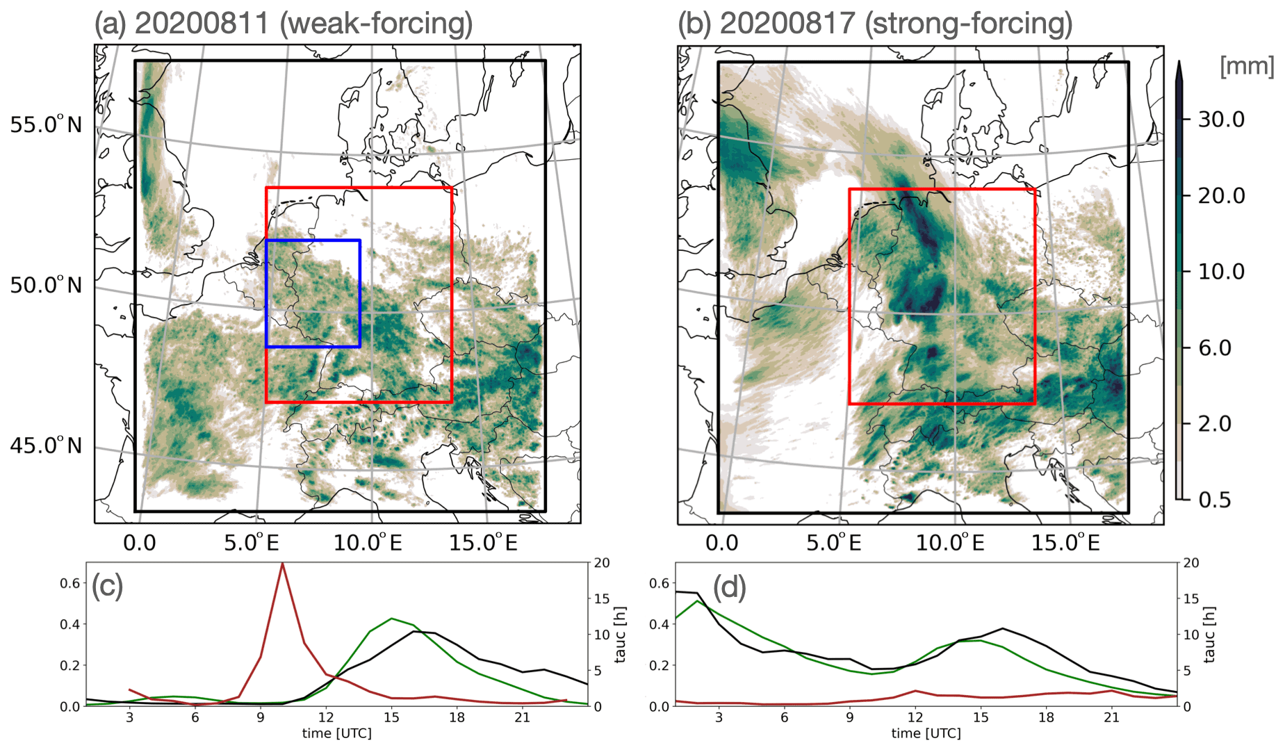
Figure 2 Daily accumulated precipitation on (a) a weakly forced day (11 August 2020) and (b) a strongly forced day (17 August 2020). Ensemble mean daily totals of the IBC sub-ensemble nu0c are shown. The black rectangles indicate the ICON-D2 simulation domain, the red rectangles depict the German domain used for evaluation, and the blue rectangle depicts the central western German domain used to inspect the spatial variability in rainfall patterns in Fig. 5. The time series of area-averaged hourly precipitation (green) and the convective adjustment timescale τ_c (red) complemented by the radar observed data (black) illustrate the different characteristics of both days in panels (c) and (d).

Table 1 List of case studies for which 180-member ICON-D2 ensemble experiments were performed, indicating the date, the type of synoptic forcing, the daily maximum convective adjustment timescale (τ_c) and daily precipitation of different IBC sub-ensemble means with their microphysical configurations.

The 17 August 2020 represents a strong forcing situation associated with a weak low-pressure system located over France that moved eastward towards Germany (not shown). The cyclonic flow favoured large-scale ascent initiating convection, especially over the western part of Germany, resulting in widespread precipitation (Fig. 2b). There was rainfall from the start of the forecast, and the heaviest rainfall occurred at night followed by a gradual reduction in precipitation until noon (green in Fig. 2d). In the afternoon, there was a secondary peak of convective precipitation between 11:00 and 18:00 UTC. The daily maximum τ_c is less than 2 h on 17 August 2020 (Table 1 and red line in Fig. 2d). Such low values indicate that CAPE was immediately consumed by a continuous triggering of convection caused by synoptically forced ascending motion characteristics in a so-called equilibrium regime.

The comparison of the precipitation time series with area-averaged radar observations indicates the realism and fidelity of the ICON-D2 ensemble forecasts (Fig. 2c and d). Characteristic values of the remaining three cases and their classification are presented in Table 1.

4 Results

To assess the relative contributions of the various uncertainties we extract different sub-ensembles from the large 180-member ensemble. First we focus on nine-member MP sub-ensembles in which each of the sub-ensemble members has different combinations of CCN and CDSD parameters but identical IBCs to examine the relative contribution of the combined microphysical (MP) perturbations on precipitation. Since there are 20 IBCs in the entire ensemble, there are 20 different MP sub-ensembles with nine members each. Likewise, there are nine 20-member IBC sub-ensembles, with one fixed combination of MP perturbations but 20 different IBCs. This different sub-sampling perspective allows conclusions to be drawn on the relative impact of IBC uncertainty. Lastly, there are 60 three-member CCN and CDSD sub-ensembles that inform about their individual contribution.

4.1 Daily area-averaged precipitation

To estimate the impact of the combined microphysical uncertainty we first focus on nine-member microphysics (MP) sub-ensembles sub-sampled from the entire 180-member ensemble. The relative differences in 24 h accumulated area-averaged precipitation forecast of all 180 ensemble members to their combined MP sub-ensemble mean are shown in Fig. 3 for a synoptically weak and a strong forcing case to contrast the flow-dependent behaviour. Every dot represents the precipitation difference in a single ICON-D2 forecast to its sub-ensemble mean. Since there are 20 different MP sub-ensembles composed of nine microphysically perturbed members (colour coded as in Fig. 1a), the 180 dots illustrate the overall variability. Apparently the impact of microphysical uncertainty is larger during weakly forced conditions, and there is surprisingly high variability between the different MP sub-ensembles, in particular during weak control. The largest and smallest range of precipitation differences amounts to 48 % (+23 % to −25 %) and 11 % (+7 % to −4 %), respectively (compare members eight and nine in Fig. 3a). During strong synoptic control the differences amount to 16 % (+9 % to −7 %) and 4 % (+2 % to −2 %), respectively (compare members 2 and 18 in Fig. 3b).

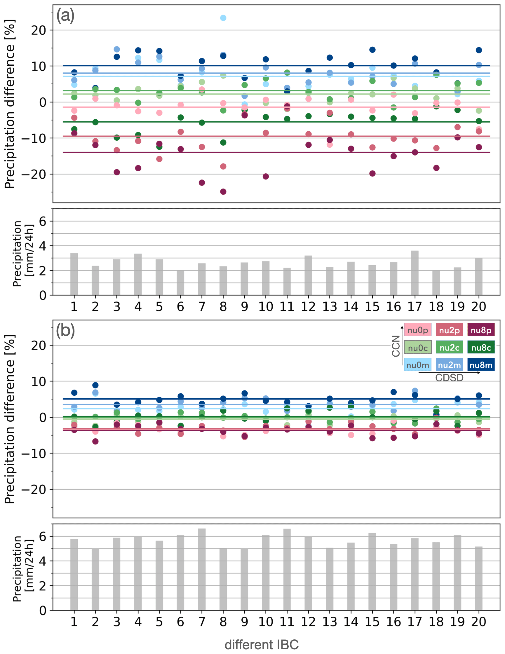
Figure 3 Relative difference in daily area-averaged precipitation (in %) with respect to combined microphysical (MP) sub-ensemble means sharing the same initial and lateral boundary conditions (IBC) for the (a) weak and (b) strong forcing cases. The columns below indicate absolute precipitation values of the 20 different MP sub-ensemble means. The nine colours indicate all combinations of microphysical configurations (as in Fig. 1a). The coloured lines show the averages.

Furthermore, it is possible to assess the different microphysical impact on precipitation. The average precipitation differences caused by MP perturbations are displayed by coloured lines in Fig. 3; for instance, experiment nu8m (narrow CDSD and maritime CCN content; dark blue) exhibits the largest precipitation deviations in both regimes. More generally, experiments with maritime aerosol load (low CCN content, blue) show an increase in precipitation, while the experiments with high CCN concentrations (polluted, red) show a decrease. Increasing the CCN concentration from maritime (nu8m) to polluted conditions with narrow CDSD shape (nu8p) amplifies average precipitation differences to +11 % and −14 % in the weak forcing case, respectively (+5 % to −4 % in the strong forcing case). A comparison between the lines having the same colours but a different darkness shows that the shape parameter of the CDSD also exhibits a systematic impact in the weak forcing situation (e.g. light red (nu0p) and dark red (nu8p) lines in Fig. 3a), whereas a CDSD's impact is hardly seen in the strong forcing situation. Narrower CDSD distributions give less precipitation, particularly during polluted conditions (nu8p, dark red). The larger sensitivity to CDSD during weak synoptic control and a systematic decrease in precipitation with increasing shape parameters are consistent with Barthlott et al. (2022a, b). During strong synoptic control the average relative difference is governed by the CCN concentration (Fig. 3b).

The governing role of IBC perturbations on precipitation is evident when comparing the sub-ensemble mean precipitation amounts of the 20 different MP sub-ensembles. During weak control, the variability ranges between 1.9 and 3.6 mm d⁻¹, whereas it ranges between 5.0 and 6.6 mm d⁻¹ during strong synoptic control (lower panels in Fig. 3). This variability is purely caused by IBC uncertainty driving the 20 different MP sub-ensembles. The similar amplitude of the variability (1.7 versus 1.6 mm d⁻¹) suggests a larger impact of IBC uncertainty during weak control when the absolute rainfall values are roughly only half as large. There is no systematic relationship between the precipitation amount and the amplitude of relative differences during both regimes. That means the microphysical impact is not constrained by daily precipitation amounts.

Interestingly, a closer inspection reveals that different IBCs can completely reshuffle the rank of the individual members in a specific MP sub-ensemble. For instance, experiments with modest aerosol content but different shapes of the CDSD show extremes for member 11 during weak control (nu8c (dark green) shows the largest negative and nu2c (medium green) shows the largest positive impact; Fig. 3a). This non-systematic and highly varying response of precipitation to perturbed microphysical parameters of individual ICON-D2 experiments points towards a strong sensitivity to IBC. This finding illustrates the necessity to be cautious when interpreting results based on a deterministic approach only to evaluate uncertainty.

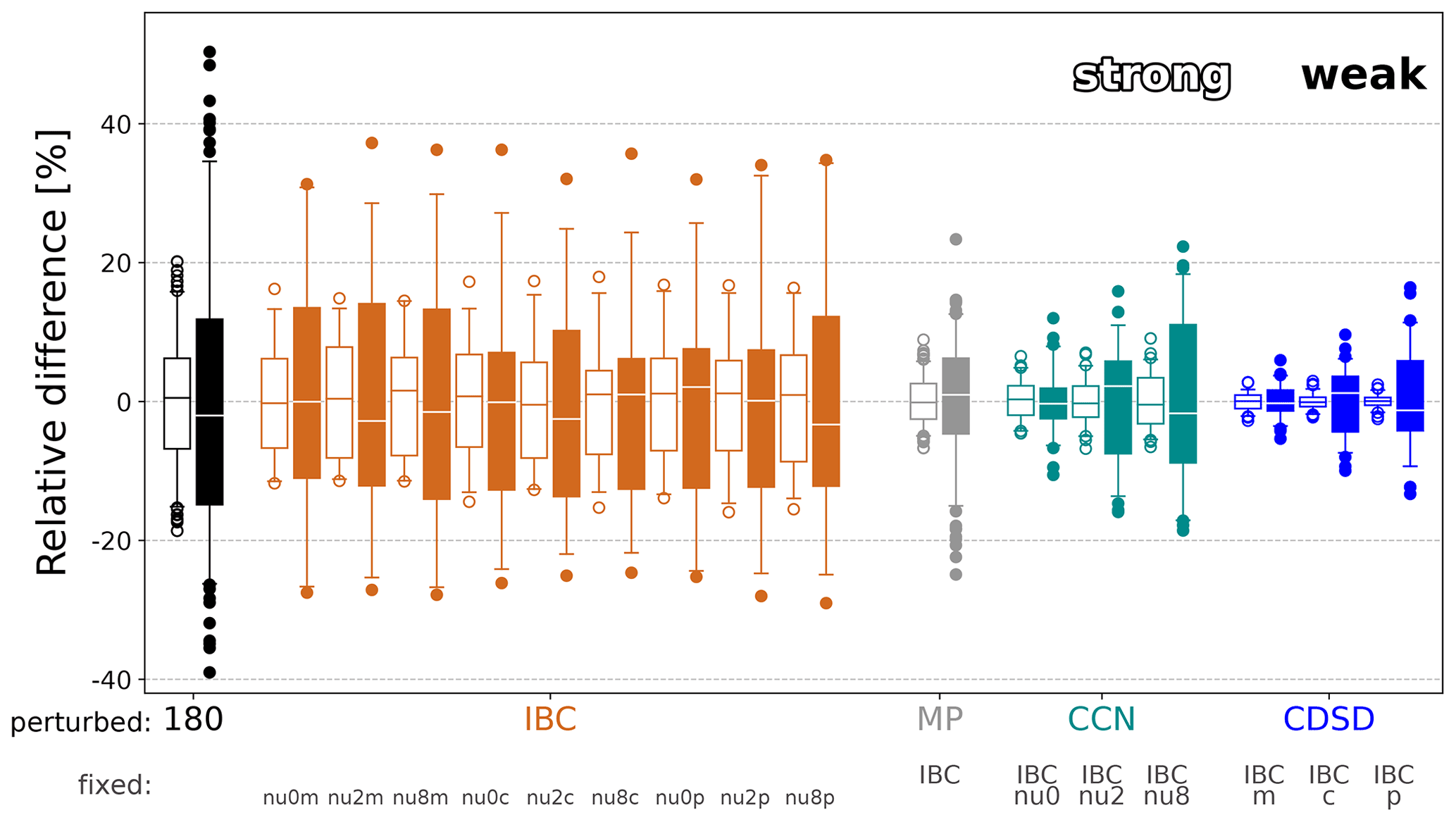
Figure 4 Box and whisker diagram showing the relative differences of daily area-averaged precipitation of individual ICON-D2 members belonging to various (sub-)ensembles. The perturbations (x labels in colour) and different fixed configurations (grey x labels) are indicated. 180 is the abbreviation of the entire ensemble and IBC, MP, CCN and CDSD are for the different sub-ensembles. The bars, boxes, whiskers and dots show medians, interquartile ranges, 5th and 95th percentiles, and outliers, respectively. Filled boxes represent weak control (11 August) and open boxes strong synoptic control (17 August).

Next, we further compress the data to directly compare and quantify the relative contribution of the various sources of uncertainty conditional on the weather regime. The resulting relative daily area-averaged precipitation differences of various sub-sampling strategies are displayed in Fig. 4. We again calculated the deviations with respect to a sub-ensemble mean; for instance, the nine different 20-member IBC sub-ensembles are shown by orange box and whisker diagrams depicting the medians, interquartile ranges, 5th and 95th percentiles, and outliers.

First, it becomes evident that the magnitude of the impact of the various uncertainties largely depends on the synoptic control. The IBC sub-ensembles show a remarkable range of +38 % to −30 % in daily precipitation sums during the weak forcing situation (filled orange dots of IBC in Fig. 4). Although their medians and interquartile ranges have some variability among the different microphysics configurations, no systematic dependence is found, and the variability between the nine IBC sub-ensembles is statistically insignificant. A corresponding behaviour is found for the strong forcing case with smaller amplitudes between +15 % and −12 % (open orange dots in Fig. 4).

Secondly, the synergistic effect of microphysical perturbations (grey in Fig. 4) ranges between +22 % and −25 % for the weak forcing case and ± 10 % for the strong forcing case. Note that the relative differences of the 20 different MP sub-ensembles (with nine members each), previously discussed in detail (Fig. 3), are collapsed into one column here.

The individual microphysical perturbations consequently result in 60 sub-ensembles (with three members each) denoted CCN sub-ensemble and CDSD sub-ensemble. Interestingly, the impact of individual CCN perturbations shows a clear dependence on the CDSD shape and vice versa. The CCN impact is smallest (± 10 %) with a broad distribution (shape parameter ν=0) and increases to a range of +22 % and −20 % with narrower distributions (increase in shape parameter). The impact of CDSD perturbations also increases with an increase in the CCN concentration. This steady increase in impact is also found in the CCN concentrations during strong forcing, while the shape of the CDSD shows a small sensitivity only. Precipitation reacts more sensitive to microphysical perturbations during weak synoptic control. In this situation, the interquartile range of the combined MP sub-ensemble (grey box) becomes smaller than those of the CCN sub-ensembles with fixed shape parameters (cyan boxes for fixed ν=2 and 8) corresponding to a narrower CDSD. Thus adding CDSD perturbations to CCN uncertainty renders the probability density function of the relative impact sharper and leads to an extension of the tails of the distribution (grey dots of MP sub-ensemble).

Finally, the 180-member ensemble including IBC and microphysical uncertainty shows the largest variability during weak control. Conditional on the weather regime the extremes in daily precipitation of individual members deviate from the ensemble mean by +50 % to −40 % with an interquartile range of ± 15 %. Interestingly the interquartile range and the 5th and 95th percentiles of the 180-member ensemble are similar to pure IBC uncertainty (compare black and orange box and whiskers). Again, microphysical uncertainty particularly affects the tails of the distribution (which are 10 % of the members represented as dots in Fig. 4).

In summary, IBC uncertainties dominate the impact on precipitation, while microphysical uncertainties play a secondary role. CCN has a larger impact than CDSD. Combined perturbations of CCN and CDSD enhance each other and show larger extremes in precipitation than individual CCN and CDSD perturbations. While the interquartile range of the 180-member ensemble and the individual IBC sub-ensembles is similar, the extreme members in the full ensemble surpass the IBC variability by +15 % and −10 %. Thus, the combination of IBC and microphysical uncertainty affects the magnitude of the extremes while keeping the interquartile range fairly unaffected.

4.2 Spatial variability based on hourly rain rates

To address the question of how IBC and microphysical uncertainties affect convective precipitation on different spatio-temporal scales, we now move from area averages to the kilometre scale and from daily to hourly accumulations. The fractions skill score (FSS; Roberts and Lean, 2008) and its variant believable scale (Dey et al., 2014; Bachmann et al., 2020) are used to objectively assess differences in spatial variability caused by different sources of uncertainty. But first we apply subjective visual inspection on selected precipitation fields to illustrate differences.

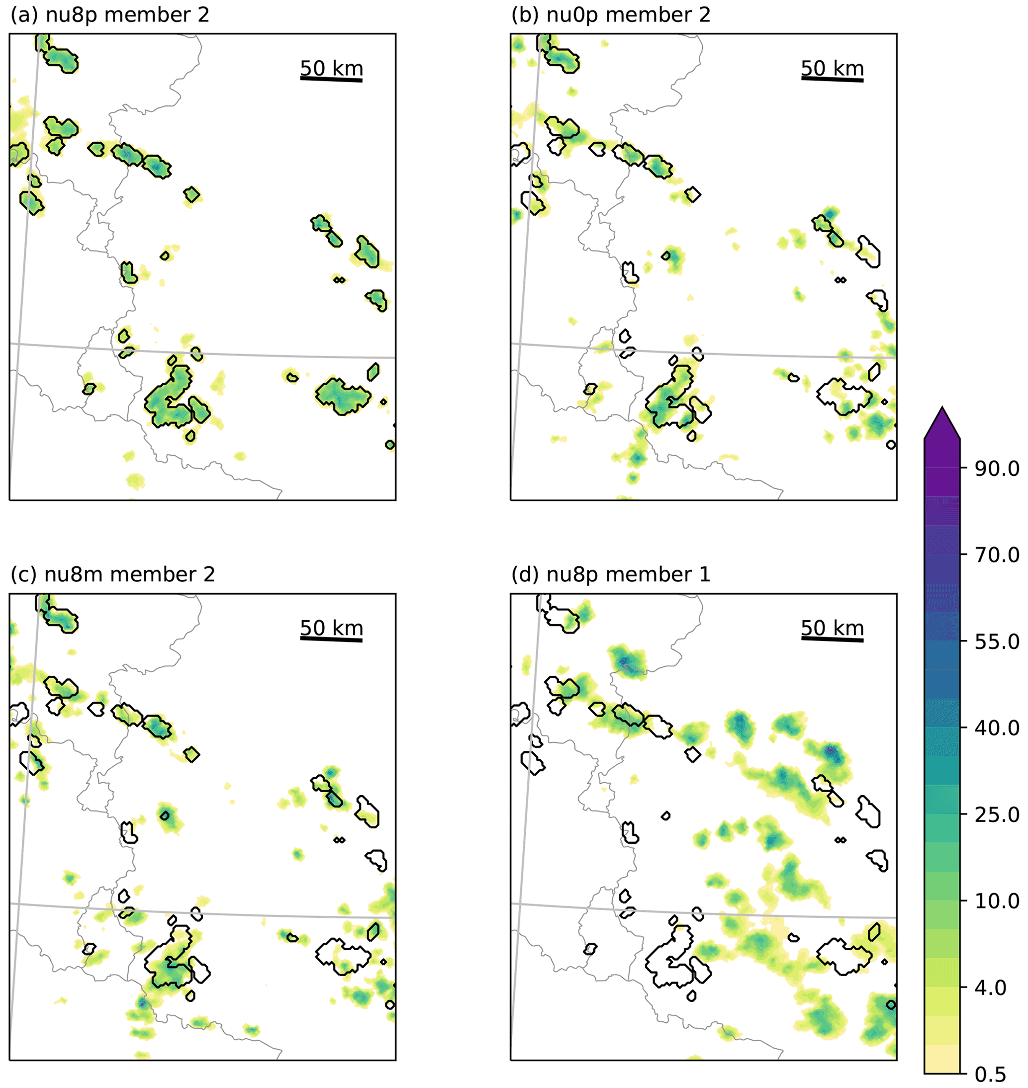
Figure 5 Snapshot of hourly precipitation at 16:00 UTC for the weak forcing case (11 August). Member 2 of IBC sub-ensembles (a) nu8p, (b) nu0p and (c) nu8m and (d) member 1 of nu8p in the central western part of Germany (see blue box in Fig. 2). Black contours indicate grid points that have a larger value than the 99th percentile value in the nu8p sub-ensemble of member 2. The red circle in (a) indicates single convective cells discussed in the text.

In Fig. 5 a snapshot of hourly precipitation over central western Germany (blue box in Fig. 2a) for the weak forcing case (11 August) at 16:00 UTC exemplifies the different impact of IBC and microphysical perturbations. This day is chosen because of the stronger impact of the perturbations during weak synoptic control, 16:00 UTC represents the time of maximum afternoon precipitation within the diurnal cycle of convective precipitation (see Fig. 2c), and the displayed sub-domain clearly depicts the typical popcorn-type precipitation structure. In Fig. 5 the transient character of individual cells is juxtaposed for four different experiments: three of them share the identical IBC (Fig. 5a–c), CCN concentration (Fig. 5a, b and d) and shape parameter of the CDSD (Fig. 5a, c and d), respectively.

At first glance, it becomes evident that the microphysical perturbations result in a similar rainfall distribution (Fig. 5a–c), whereas the member driven with different IBCs shows a considerably different rainfall field (Fig. 5d). The direct comparison of the location of intense precipitation caused by the different perturbations relative to the 99th percentile of simulation nu8p (black contours in Fig. 5) shows that convective cells of simulations nu0p (broad CDSD, polluted) and nu8m (narrow CDSD, maritime) are either at the same location or in close vicinity. Some weak rain cells (e.g. southeast of Luxembourg; red circle in Fig. 5a) are intensified by decreasing CCN and shape parameters of the CDSD, thus in agreement with the spatio-temporal integrated rainfall signal discussed in the previous section. Positions of strong rain cells are shifted by the CCN perturbation at a scale of 20–30 km, whereas an increase in the shape parameter of the CDSD hardly shows a clear impact. The visual inspection of many scenes of hourly rainfall caused by convective cells confirms the systematic behaviour of microphysical perturbations with stronger precipitation with low CCN concentration and broad CDSD shapes (not shown).

To briefly summarise the visual inspection, we can state that in polluted CCN conditions both CCN and CDSD perturbations impact the spatial variability at almost the same scale. While microphysical perturbations keep the general spatial structure, IBC perturbations largely alter the position of convective cells. Thus microphysical perturbations primarily impact the precipitation amount by changing the precipitation intensity rather than by feedback on dynamical fields and triggering new cells. Visual inspection of rainfall patterns of the strong forcing case results in similar findings: minor shifts of rain cells in microphysics sub-ensembles and a smaller impact of CDSD perturbations (not shown).

To quantify the spatial (dis-)agreement of hourly precipitation fields in the various simulations we employ the FSS, a spatial score that shows the similarity between two binary fields (denoted A and B, two distinct sub-ensemble members in our case) within a predefined neighbourhood scale. The definition of the FSS is given by

$$\begin{array}{}\text{(2)}& \text{FSS}=\mathrm{1}-{\displaystyle \frac{\sum (f_A-f_B{)}^{\mathrm{2}}}{\sum f_A^{\mathrm{2}}+\sum f_B^{\mathrm{2}}}},\end{array}$$

where f_A and f_B represent the fraction of rainy grid points in fields A and B, respectively, at which the precipitation amount is above a certain threshold value. The second term on the right-hand side is the ratio of the mean squared error (MSE) of the fraction fields A and B to the maximum possible MSE (Roberts and Lean, 2008). If the number of grid points with a value of 1 within a certain neighbourhood of a grid point is equal between two fields, the FSS is 1.0, which means the compared two fields are identical. FSS becomes smaller as the difference between two fields gets larger, and it becomes 0.0 when only one of the fields has values and the other has a complete miss in the respective neighbourhood. In this study, we use the 99th percentile of hourly precipitation as the threshold to generate a binary field to take into account the strong diurnal cycle of rainfall intensity and to keep the number of grid points used for FSS calculation constant. The 99th percentile is useful to capture the position of convective cells (see contours in Fig. 5). The FSS is calculated over Germany with neighbourhood sizes varying from 2.2 km (1 grid point) to 563.2 km (256 grid points). Since FSS is a score calculated between two fields, we need to carefully consider how to compute an ensemble FSS. Following Dey et al. (2014), we calculate the FSS for all combinations of ensemble members belonging to a sub-ensemble. For instance, FSSs for an IBC sub-ensemble (with 20 different IBCs) can be calculated as 20 ⋅ $\mathrm{19}/\mathrm{2}$ = 190 times. Since there are nine IBC sub-ensembles in this study, the number of overall FSSs that shows the impact of IBC perturbations is 190 ⋅ 9 = 1710. Accordingly, the numbers of FSSs for combined microphysics, CCN and CDSD sub-ensembles are 720, 180 and 180, respectively. Mean values of the FSSs are shown in Figs. 6 and 7 to objectively represent the spatial variability given by various kinds of uncertainties.

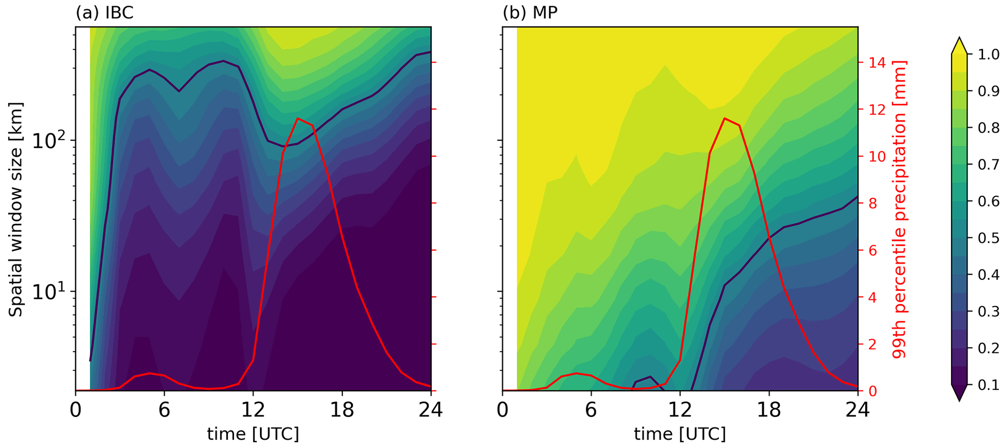
Figure 6 Ensemble mean FSS values of hourly precipitation calculated across scales ranging from 2 to 560 km in the German domain for the weak forcing case of 11 August. The IBC sub-ensembles' mean FSS is depicted in panel (a) and the combined microphysics sub-ensembles' mean FSS in panel (b). The black lines show believable scales of mean FSS. The red lines (right axis) show the time series of the mean 99th percentile value of hourly precipitation.

Figure 7 As Fig. 6 but for the (a) CDSD, (b) CCN and (c) WNoise sub-ensembles.

In addition, we use the believable scale (Dey et al., 2014; Bachmann et al., 2020) to characterise a typical length scale that estimates the spatial difference between two fields. The believable scale is defined as the neighbourhood size when the FSS exceeds a threshold defined by $\text{FSS}\ge \mathrm{0.5}+\frac{f_{\mathrm{0}}}{\mathrm{2}}$, where f₀ is the fraction of grid points considered in the FSS calculation (the 99th percentile threshold gives f₀=0.01). Since the FSS is applied on precipitation fields above the 99th percentile values, the believable scale can be considered in this study as a scale showing how large a mismatch of intense convective cells is.

Time–space diagrams of the ensemble mean FSSs given by IBC and combined microphysical uncertainty are depicted in Fig. 6 for the weak forcing case. Low FSS values represent large spatial deviations between the location of intense convection, hence a larger spatial variability. The variability due to the IBC perturbations is considerably larger than the one forced by combined microphysical perturbations. However, and typical for days with weak control, convective precipitation only forms in the late morning (see, for example, time series in Fig. 2c and red line depicting the 99th percentile of hourly precipitation in Fig. 6). The value of the 99th percentile of hourly precipitation amounts to 1 mm h⁻¹ at 12:00 UTC, and precipitation is mostly negligible before. Interestingly, at the onset of convective precipitation at 12:00 UTC the believable scale exhibits a dip, and the spatial variability decreases to slightly less than 100 km and thereafter continuously increases throughout the convective period until the evening. The reduction in the spatial variability in the afternoon, representing co-locations of convective cells, is constrained by steady, non-perturbed factors forcing the dynamical fields involved in cloud and precipitation formation like orography. After 22:00 UTC the hourly precipitation rates amount again to less than 1 mm h⁻¹, and the corresponding believable scale exceeds 200 km like before the onset of convection at night and in the morning. In contrast, the spatial disagreement caused by combined microphysical perturbations is smaller, and the mean believable scale amounts to only 16 km at the peak of precipitation at 16:00 UTC (Fig. 6b). Apparently, the impact of microphysical perturbations on precipitation acting on many pathways needs time and starts at a much lower spatial scale than IBC perturbations.

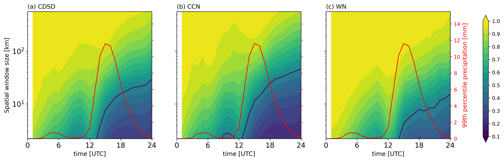
At first sight, individual perturbations of CCN and CDSD show a similar growth of FSS as the combined microphysical perturbations (Figs. 6b and 7). Close inspection reveals that the believable scale of precipitation caused by CCN perturbations (black line in Fig. 7b) starts to increase at the onset of the precipitation (at 12:00 UTC), 1 h before that of the CDSD perturbations (Fig. 7a). The CDSD believable scale grows more slowly and is always smaller (roughly 50 %) than that of combined microphysical perturbations. Since changes in CCN have a direct influence on the cloud condensation process, while the shape parameter of the CDSD affects ensuing microphysical processes, this time shift is plausible. Interestingly, the CCN-perturbed believable scale reaches 40 km after 22 h, the same length scale as the believable scale of the combined microphysical perturbations. In contrast to the impact on precipitation amount, combining two sources of microphysical uncertainty does not increase the spatial variability.

The uncertainty of CCN concentrations has a larger impact than the shape parameter of the CDSD on the spatial variability in intense precipitation cells. Now we can ask if this behaviour is by chance and if this finding holds for other thresholds or percentiles, respectively. For this reason, we performed additional white noise (WNoise) ensemble simulations with 20 different IBCs but only for the “default” microphysics configuration (nu0c) to examine whether the spatial variability caused, for instance, by microphysical perturbations differs from the impact of random, tiny differences in the temperature field. Following the method of Selz and Craig (2015) the virtual potential temperature field is perturbed by a non-biased Gaussian noise with a standard deviation of 0.01 K at all grid points of the entire model atmosphere at an initial time. The comparison of the microphysically perturbed ensemble with a pure white noise (WNoise) experiment shows a similar onset and increase in spatial variability (Fig. 7c). The spatial variability caused by CCN and CDSD perturbations is, however, larger than the effect of the WNoise perturbations. At 16:00 UTC, the mean FSS of WNoise simulations is close to 1 at scales larger than 80 km, and the believable scale is about 5 km. Thus the effect of microphysical uncertainty on the spatial precipitation fields is systematically exceeding the effect of tiny errors at the initial time in the WNoise experiment. Less intense precipitation cells detected by the 95th percentile threshold indicate a similar albeit slightly smaller variability due to IBC and microphysical perturbations (not shown). Using a 90th percentile threshold on hourly precipitation results in values lower than 0.1 mm at all forecast hours and gives no extra information.

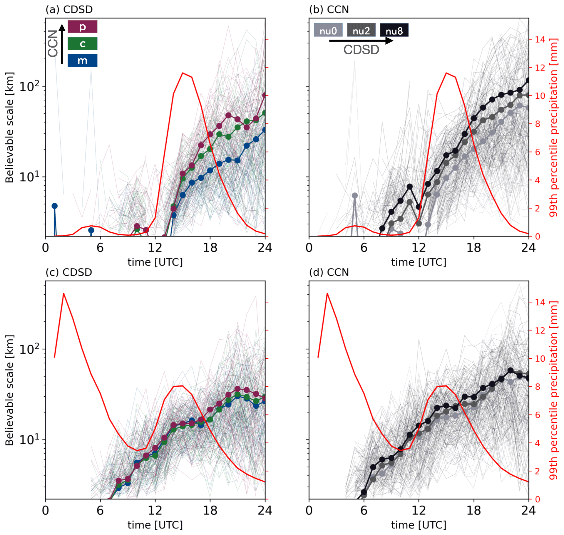
Figure 8 Time series of FSS believable scales of hourly precipitation for every combination of (a) the CDSD and (b) CCN sub-ensemble for the weak forcing case in the German domain. In (a) blue, green and red lines indicate simulations with maritime, continental and polluted CCN content, respectively. In (b) light grey, dark grey and black lines indicate scales with the broad, intermediate and narrow CDSD. Bold lines with circles indicate mean values of FSS believable scales sharing the same perturbation. The red lines (right axis) show time series of the mean 99th percentile value of hourly precipitation. Panels (c) and (d) show the results for the strong synoptic forcing case.

To further elucidate the combined microphysical perturbations and the interdependence of one perturbation (say CCN) when the other (CDSD) is kept constant in the presence of IBC uncertainty, time series of all believable scales calculated between every combination of ensemble members are illustrated in Fig. 8. The bold lines in Fig. 8a clearly reveal that CDSD perturbations result in spatial variability at different length scales depending on a certain fixed CCN concentration during weak synoptic control. In clean air conditions (maritime aerosol content; dark blue lines in Fig. 8a), the mean believable scale attains 10 km roughly 3 h after the onset of the believable scale's growth. At 22:00 UTC, towards the end of the diurnal cycle, the value increases to 15 km. On the other hand, for polluted conditions (dark red and green lines), the mean believable scales attain larger values: 15 km at 16:00 UTC and 30 to 40 km at 22:00 UTC. The mean length scale of disagreement given by the CDSD perturbations in polluted conditions (high CCN concentrations) is twice as large as in clean conditions (low CCN concentrations). Note, however, that there is large variability among pairs of ensemble members, and hence the IBC dependence is larger than the impact of the background CCN condition. A similar systematic dependence can be found for the CCN perturbations' impact with different fixed CDSD shape parameters. The mean believable scale with the broadest CDSD (lightest grey lines in Fig. 8b) reaches 10 km at 16:00 UTC and 50 km after 22 h of lead time. With the narrowest CDSD (black lines), the mean believable scale of CCN perturbations is 20 km at 16:00 UTC and increases to 100 km later. Interestingly, the mean believable scale with the narrowest CDSD is by a factor of 2 larger than the broadest CDSD. This relationship is similar to that found in spatially averaged precipitation amounts; namely polluted CCN and narrow CDSD conditions lead to larger variability (Fig. 4).

In strong synoptic control, the situation is slightly different (Fig. 8c and d). The believable scales only start to grow from 07:00 UTC onwards, and the mean values finally reach a neighbourhood size of 30 km at 22 h lead time. This monotonic pattern of the perturbation growth is similar to the weak forcing case. However, the mean believable scale for clean CCN conditions is larger than for the weak forcing case at 22:00 UTC (bold dark blue lines in Fig. 8a and c). There is no systematic difference in the mean believable scale caused by CDSD perturbations in the presence of various yet fixed CCN concentrations (Fig. 8c). On the other hand, given narrower CDSDs, the CCN perturbations cause a slightly larger spatial variability (Fig. 8d). Nevertheless, the difference between the broadest and narrowest CDSD simulations is less pronounced in comparison to the weak forcing case (10–15 km difference in strong control versus 30 km in weak control at 22:00 UTC). It is interesting to note that the impact of the microphysical perturbations on the spatial precipitation pattern only starts to appear in FSS after 7 h of lead time, although there is continuous rainfall from forecast initialisation during the strong forcing case. In the first hours of the simulation spin-up effects and the adjustment to the driving coarser-scale model are still at work, which dampens the impact of the microphysical uncertainties (see, for example, Barthlott et al., 2022a). Thus, microphysical perturbations need a longer spin-up time than IBC perturbations to modulate dynamical fields, eventually resulting in precipitation at different locations (see Fig. 8c and d).

Note that there is a difference between the believable scale of a “mean FSS” (e.g. black line in Fig. 6) that represents a scale of (dis-)agreement given, say, an ensemble mean FSS value and the mean over many believable scale values of paired member-to-member comparisons (Fig. 8). The ensemble mean FSS is useful for an intercomparison of the average impact given by different perturbations in general, whereas the mean of member-to-member believable scales (Fig. 8) provides a scale of actual (dis-)agreement of certain scenes, for example, the precipitation patterns shown in Fig. 5.

4.3 Relative impact on cloud and rainwater content

To complement the assessment centred on the relative impact on precipitation, we now turn to important precursors in the complex process chain to form precipitation and inspect the contribution of the uncertainties to the cloud and rainwater content within a full convective-scale EPS framework. Since we find similar systematic responses in both weather situations, we show results for the weakly forced case only. In Fig. 9 we depict the variability caused by IBC uncertainty in clouds and rainwater. The 24 h mean of hourly values is computed for the nine different IBC sub-ensembles to examine the relative impact.

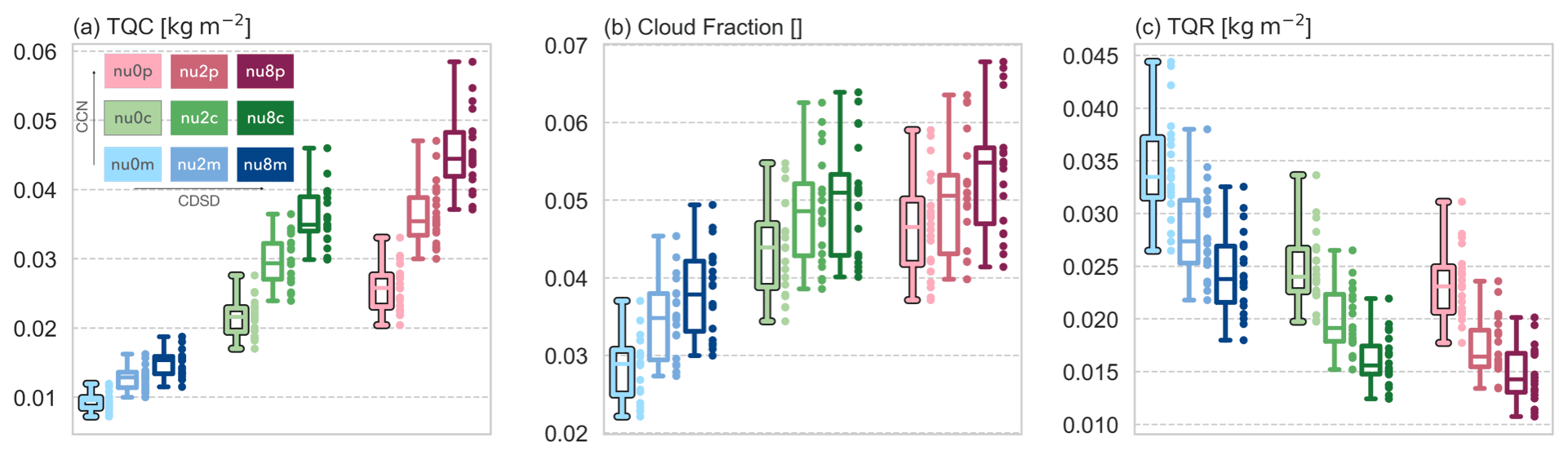
Figure 9 Box and swarm plots for 24 h mean (a) domain-averaged total column cloud water content, (b) cloud fraction and (c) domain-averaged total column rainwater content over Germany for the weak forcing case. The box plots and dots illustrate the same dataset, but the dots represent individual IBC sub-ensemble members. The colours are based on the various combination of microphysical perturbations shown in Fig. 1a. Box plots show medians, interquartile ranges, and maximum and minimum values in that order.

The vertically integrated cloud water content (TQC) increases significantly with higher CCN concentration and CDSD shape (Fig. 9a). The medians of the ensembles with different microphysics uncertainty vary by more than 400 % (TQC is amounting to 0.01 kg m⁻² in experiment nu0m and 0.044 kg m⁻² in nu8p). The comparison of sub-ensembles sharing identical CDSD shape parameters shows an increase in TQC of up to 300 % when increasing CCN concentrations from maritime to polluted conditions (compare experiments nu0m and nu0p in Fig. 9a). Similarly, the change from the broadest to the narrowest CDSD enhances TQC by roughly 150 %. These values are more than an order of magnitude larger compared to the impact of microphysical perturbations on precipitation (compare to orange IBC sub-ensembles in Fig. 4). An important implication seen in Fig. 9a is that IBC perturbations cannot encompass the variability caused by microphysical uncertainties in cloud forecasts, which manifests by marginal (or no) overlap of the distributions which have different CCN and CDSD configurations (differently colour-coded in Fig. 9).

The forecast cloud fraction also systematically increases with higher CCN and shape parameters (Fig. 9b), in agreement with the increase in TQC. Cloudy grid points are defined as grid cells where TQC > 50 g m⁻². The medians of the cloud fraction in IBC sub-ensemble nu0m (light blue), nu8m (dark blue), nu0p (light red) and nu8p (dark red) are 0.29, 0.39, 0.47 and 0.55, respectively. Thus, cloud fraction increases with higher CCN and/or CDSD parameters by 35 %, 62 % and 91 % relative to experiment nu0m. Compared to TQC, a change in CDSD shape parameters shows an only minor effect on cloud fraction in continental and polluted CCN conditions (e.g. nu8c and nu8p in Fig. 9b). This is presumably caused by ambient atmospheric conditions as, for example, humidity sets an upper bound for total cloud cover. Hence microphysical uncertainty (CCN and CDSD perturbations) becomes less important, and IBC uncertainty, which predominantly triggers convection and determines the upper bound of cloud coverage, governs the variability in spatial cloud distributions.

Finally, the vertically integrated rainwater content (TQR) averaged over Germany shows a systematic but opposite response compared to TQC (Fig. 9c). TQR decreases with increasing CCN and shape parameters of the CDSD and parallels the systematic impact found for precipitation. Compared to TQC the variability caused by microphysical perturbations becomes smaller; for instance, the TQR median of experiment nu0m amounts to 0.033 kg m⁻² and nu8p to 0.014 kg m⁻², indicating a decrease by roughly 58 %.

The steady decreasing systematic impact of the microphysical uncertainty on cloud water content, rainwater content and eventually precipitation hints towards some kind of buffering effects or compensating processes that reduce the large, positive impact on clouds and eventually even turn it into a negative impact with respect to rain production. Companion work by Barthlott et al. (2022a, b) and Baur et al. (2022) shed light on those processes. One major process is the reduction in warm rain processes. The suppression of collisional growth of cloud droplets in polluted CCN conditions reduces the formation of raindrops, and small droplets become more likely to evaporate. Moreover, cloud optical properties are influenced as well through changes in the droplet's effective radius. That, in turn, can affect the radiative energy supply that triggers new convection.

4.4 Quantification of relative impact based on 5 d

Finally, we repeat the analysis and use 180-member ICON-D2 ensemble experiments performed for 5 d in August 2020 to confirm the previous findings. The classification into distinct weather situations with different synoptic control results in three weakly and two strongly forced cases (see Table 1). The regime-dependent relative impact of the various perturbations is computed as follows: first, the relative difference in every individual member to its corresponding sub-ensemble mean is calculated separately for every day (as in Sect. 4.1 and displayed in Fig. 4). Secondly, the median, the interquartile range, and the 5th and 95th percentiles are computed by aggregating the days for each synoptic forcing separately (i.e. 540 samples for weak and 360 for strong forcing). Finally, the samples are bootstrapped 100 times with replacement to get robust results, and the mean of the 100 medians, interquartile ranges and percentile values are finally depicted in Fig. 10. This procedure takes into account the different mean values of distinct sub-ensembles on different days (see Table 1) and allows a fair comparison. The 5th and 95th percentiles of the relative difference then define the 90 % confidence interval (similar to Craig et al., 2022).

Figure 10 Relative differences in the 180-member ensemble (black), the averaged IBC sub-ensembles (orange) and averaged combined microphysical sub-ensembles (grey) aggregated over 5 d in August 2020 conditional on synoptic control. Relative differences in precipitation, total column rainwater content (TQR) and total column cloud water content (TQC) are displayed using filled boxes for weak forcing situations. Box plots show bootstrapped medians, interquartile ranges, and the 5th and 95th percentiles in that order. For details see the text.

In the full 180-member ensemble, including IBC and combined microphysical uncertainties, the confidence interval of precipitation deviates for individual experiments from the ensemble mean by +41 % to −32 %, with an interquartile range between +15 % to −18 % during weak forcing. The corresponding impact of pure IBC perturbations shows a range of +36 % to −29 % during weak forcing (orange boxes of IBC sub-ensemble in Fig. 10). The variability is smaller and amounts to ±23% during strong forcing. The medians have a slightly negative bias for the weak forcing cases because the precipitation distribution is slightly positively skewed; i.e. the mean is larger than the median. That might be an artefact of the given sample size.

The impact of combined microphysical perturbations on the confidence interval of precipitation (grey bars in Fig. 10) varies between +12 % and −13 % in weak forcing cases and ± 6 % during strong forcing cases. Thus precipitation amounts are twice as sensitive to pure microphysical perturbations during weak control. Adding microphysical perturbations to the IBC sub-ensembles (giving the full 180-member ensemble) shows a negligible impact on the interquartile range (compare black and orange bars in Fig. 10) but extends the tails of the distribution (black and orange whiskers in Fig. 10) by 5 % for weak forcing conditions.

The same methodology is applied to convective clouds represented by averaged vertically integrated rainwater content (TQR in Fig. 10). Microphysical perturbations show a larger impact than IBC perturbations. The confidence interval of the impact of microphysical perturbations on TQR ranges between +54 % and −30 % for strong forcing and between +57 % and −35 % for weak forcing. Forecast variability is increased by +31 % compared to the pure IBC impact when taking the microphysical uncertainties into account, too. The relative impact of IBC perturbations on TQR ranges between +31 % and −25 % for weak forcing and between +17 % and −16 % for strong forcing.

Finally, the impact on vertically integrated cloud water content (TQC in Fig. 10) shows less dependence on synoptic control than those on rainwater or precipitation. Microphysical perturbations show a large impact on TQC, and their impact exceeds the impact of IBC uncertainty. The relative impact of microphysical perturbations on TQC ranges between +80 % and −62 % for weak forcing and between +66 % and −60 % for strong forcing. Forecast variability is increased by +47 % compared to the pure IBC impact when taking the microphysical uncertainties into account. The variability in CCN and CDSD plays a larger role in narrower CDSD or higher CCN conditions (not shown), similar to the impact on precipitation discussed in Fig. 4.

Overall, microphysical uncertainty plays a more important role in the prediction of cloud and rainwater content than IBC uncertainty, but the impact is buffered during warm rain processes. The buffering effect that counteracts microphysical perturbations discussed in Sect. 4.3 can thus be quantified. The microphysical impact on the 95th percentile value decreases from +79 % for TQC to +57 % for TQR and to +12 % for precipitation. We find a systematically larger impact of the various uncertainties for precipitation, TQR and TQC during weak forcing conditions.

5 Summary and concluding remarks

The relative importance of microphysical uncertainties in cloud and precipitation forecasts in a full convective-scale EPS framework is assessed on different spatial and temporal scales conditional on synoptic control in central Europe. In the present study, we perturb two microphysical parameters that are poorly constrained by observations. Those constitute the cloud condensation nuclei (CCN) concentration and the shape parameter of the cloud droplet size distribution (CDSD), both currently not perturbed in operational ICON-D2 ensemble forecasts. An examination of the synergistic effect of these microphysical perturbations necessitates the use of the two-moment bulk microphysics scheme of Seifert and Beheng (2006) that predicts next to the mass concentration of different hydrometeors their number density and thus allows the calculation of the particle size distribution. Their individual and combined relative impact is estimated in the presence of initial and boundary condition uncertainty (IBC) available from operational ensemble forecasting at Deutscher Wetterdienst. Nine different set-ups of such combined microphysical perturbations run with 20 different IBCs add up to 180-member ICON-D2 ensemble forecasts. The relative impact of the various uncertainties is quantified by selecting different sub-ensembles that are sharing a common uncertainty.

Based on five real summertime cases we find that the impact of the various uncertainties on precipitation crucially depends on the synoptic control. It is larger during weakly forced situations. The IBC uncertainty accounts for most of the precipitation variability. The confidence interval (that is given by the 5th and 95th percentiles) of the relative impact on daily area-averaged precipitation of individual ICON-D2 experiments ranges between +38 % and −32 % during weak forcing and ± 23 % during strong forcing (Fig. 10). Combined microphysical perturbations show a relative impact on precipitation as the confidence interval varies between +12 % and −13 % during weak forcing and only ± 6 % during strong synoptic control. Thus precipitation amounts are twice as sensitive to pure microphysical perturbations during weak control. The joint effect of IBC and microphysical uncertainty extends the tails of the forecast distribution by 5 % in weakly forced conditions. Individual ICON-D2 members exceed the ensemble mean precipitation by 50 %. However, the interquartile range of the full ensemble only marginally deviates from the pure IBC sub-ensembles (Fig. 4).

The in-depth analysis of the weakly forced case further points towards a synergistic effect of CCN and CDSD perturbations that show a large sensitivity to the other background (fixed) microphysics choice. That stems from the systematic behaviour of the responses to different microphysics conditions. Both microphysical perturbations have a systematic impact on the intensity and location of individual convective cells identified in the present study with hourly rain rates, and its spatial variability amounts to O(10 km) quantified with FSS believable scales. In contrast, IBC perturbations scramble the precipitation pattern during weak control and result in twice the location uncertainty. This suggests that microphysical perturbations have systematic effects, whereas IBC perturbations are likely to have stochastic effects. CCN perturbations cause a larger impact on spatial variability in precipitation forecasts than CDSD. Individual perturbations of CCN and CDSD have larger impacts when the other configuration is the narrower CDSD or polluted CCN condition, respectively.

Clouds react differently to the various uncertainties. The combined microphysical perturbations largely determine the variability in daily and area-averaged vertically integrated cloud water content (TQC in Fig. 10). Different from their impact on precipitation, the increase in CCN concentration and shape parameter of the CDSD has a large positive impact on the production of cloud and rainwater content forming horizontally larger clouds. Further, this impact is fairly independent of weather regime. Thus the considerable impact on cloud variables does not directly translate into precipitation amounts. This suggests that there are some microphysical processes or feedback mechanisms involved that compensate and ultimately reverse the impact of microphysical perturbations on clouds and precipitation. The systematic behaviour of cloud variables is consistent with previous studies (Seifert et al., 2012; Igel and van den Heever, 2017a; Wellmann et al., 2020; Zhang et al., 2021), and further discussion about the detailed processes seen from the deterministic perspective can be found in Barthlott et al. (2022a, b) and Baur et al. (2022). Note that we compare rainfall accumulations at the ground with averages of 24 hourly snapshot scenes of vertically integrated cloud and rainwater to facilitate a comparison of the respective contribution.

Importantly, a close inspection of the impact of microphysical uncertainties in the presence of different IBCs on precipitation indicates a strong sensitivity to IBC uncertainty (Fig. 3). This illustrates the necessity to be cautious when interpreting results based on a deterministic approach only to evaluate impact of uncertainty. The use of a full ensemble modelling framework including various key sources of uncertainty as done in this study is essential to assess their relative importance. This issue becomes even more relevant when inspecting smaller spatial and temporal scales. Another major conclusion is the necessity to take the atmospheric state into account when quantifying the contribution of various uncertainties. Given that roughly 20 % to 40 % of the days with summertime precipitation in central Europe are classified as being weakly controlled (Zimmer et al., 2011; Kühnlein et al., 2014), the considerable impact during these conditions is usually veiled when inspecting results independent of the synoptic control. A limitation of this study is the limited dataset covering 5 d in August 2020 only. More robust results require a larger database containing more cases that comprise different synoptic conditions. Based on the five cases we cannot draw general conclusions. However, we believe that the findings are robust enough to provide a scientific basis for future research.

Our results suggest that the consideration of CCN and CDSD uncertainties increases precipitation variability and can contribute to the reduction of the long-standing issue of underdispersion of near-surface variables in convective-scale EPS forecasts (see references in, for example, Keil et al., 2019) and thus ultimately benefit the improvement of NWP ensemble forecasting. It is beyond this study to assess to what extent the microphysical perturbations contribute to a better probabilistic forecasting skill compared to observations. Given the increasing importance of satellite observations used in convective-scale data assimilation, the systematic impact of microphysical uncertainties will attract interest in future. Microphysical uncertainties strongly influence forecasts of cloud coverage and droplet sizes, both representing important ingredients used in satellite forward operators to compute synthetic reflectances (e.g. Scheck et al., 2020) to be used in data assimilation algorithms.