Twenty-first-century Southern Hemisphere impacts of ozone recovery and climate change from the stratosphere to the ocean

Changes in stratospheric ozone concentrations and increasing concentrations of greenhouse gases (GHGs) alter the temperature structure of the atmosphere and drive changes in the atmospheric and oceanic circulation. We systematically investigate the impacts of ozone recovery and increasing GHGs on the atmospheric and oceanic circulation in the Southern Hemisphere during the twenty-first century using a unique coupled ocean–atmosphere climate model with interactive ozone chemistry and enhanced oceanic resolution. We use the high-emission scenario SSP5-8.5 for GHGs under which the springtime Antarctic total column ozone returns to 1980s levels by 2048 in our model, warming the lower stratosphere and strengthening the stratospheric westerly winds. We perform a spatial analysis and show for the first time that the austral spring stratospheric response to GHGs exhibits a marked planetary wavenumber 1 (PW1) pattern, which reinforces the response to ozone recovery over the Western Hemisphere and weakens it over the Eastern Hemisphere. These changes, which imply an eastward phase shift in the PW1, largely cancel out in the zonal mean. The Southern Hemisphere residual circulation strengthens during most of the year due to the increase in GHGs and weakens in spring due to ozone recovery. However, we find that in November the GHGs also drive a weakening of the residual circulation, reinforcing the effect of ozone recovery, which represents another novel result. At the surface, the westerly winds weaken and shift equatorward due to ozone recovery, driving a weak decrease in the transport of the Antarctic Circumpolar Current and in the Agulhas leakage and a cooling of the upper ocean, which is most pronounced in the latitudinal band 35–45^∘ S. The increasing GHGs drive changes in the opposite direction that overwhelm the ozone effect. The total changes at the surface and in the oceanic circulation are nevertheless weaker in the presence of ozone recovery than those induced by GHGs alone, highlighting the importance of the Montreal Protocol in mitigating some of the impacts of climate change. We additionally compare the combined effect of interactively calculated ozone recovery and increasing GHGs with their combined effect in an ensemble in which we prescribe the CMIP6 ozone field. This second ensemble simulates a weaker ozone effect in all the examined fields, consistent with its weaker increase in ozone. The magnitude of the difference between the simulated changes at the surface and in the oceanic circulation in the two ensembles is as large as the ozone effect itself. This shows the large uncertainty that is associated with the choice of the ozone field and how the ozone is treated.

1 Introduction

Ozone depletion has been the major driver of change in the Southern Hemisphere (SH) atmospheric circulation during the last decades of the twentieth century (e.g., Polvani et al., 2011b). The effects of ozone depletion extend from the stratosphere (e.g., McLandress et al., 2010; Keeble et al., 2014), where the ozone hole is located, down to the surface and to the ocean circulation (e.g., Thompson et al., 2011; Previdi and Polvani, 2014; Ferreira et al., 2015). A decline in the absorption of shortwave (SW) radiation associated with ozone depletion in the past led to the cooling of the Antarctic lower stratosphere in austral spring, which in turn resulted in the acceleration of the stratospheric westerly winds (Thompson and Solomon, 2002; Gillett and Thompson, 2003) and a delay in the breakdown of the polar vortex (e.g., Waugh et al., 1999; Langematz et al., 2003; McLandress et al., 2010; Keeble et al., 2014). At the same time, the summer Brewer–Dobson circulation (BDC) in the SH has strengthened in response to changes in wave activity associated with the delayed breakdown of the polar vortex (Li et al., 2008, 2010; Oberländer-Hayn et al., 2015; Abalos et al., 2019). The impact of ozone depletion on the westerlies extends to the surface, where the midlatitude jet strengthens and shifts poleward during the austral summer, and the Southern Annular Mode (SAM) experiences a shift towards more positive values (Gillett and Thompson, 2003; Thompson and Solomon, 2002; Son et al., 2010; Thompson et al., 2011). The associated shift in the southern storm track resulted in precipitation changes (Polvani et al., 2011b), extending to the subtropics (Kang et al., 2011). In addition, the edge of the Hadley cell shifted poleward (Son et al., 2010; Polvani et al., 2011b; Min and Son, 2013; Waugh et al., 2015), causing an expansion of the subtropical dry zones in the SH.

The impacts of ozone depletion are also felt by the ocean as the wind stress over the Southern Ocean increases. In response, the northward Ekman transport across the Southern Ocean increased, leading to enhanced divergence (convergence) and upwelling (downwelling) to the south (north) of the maximum westerly wind stress, therefore enhancing the ventilation of the Southern Ocean (e.g., Waugh et al., 2013). These changes in ocean circulation, possibly in combination with changes in surface heat fluxes, led to changes in surface and subsurface temperatures (Ferreira et al., 2015; A. Solomon et al., 2015; Li et al., 2016, 2021; Seviour et al., 2016). Coupled climate models simulate a two-stage response to a sudden stratospheric ozone loss: cold (warm) sea surface temperature (SST) anomalies occur south (north) of 50^∘ S in a fast response caused by advection due to anomalous Ekman transport, followed by a widespread warming of the Southern Ocean, in a slow response caused by anomalous upwelling (Ferreira et al., 2015; Seviour et al., 2016). There are, however, large intermodel differences in the magnitude and timescale of these responses (Seviour et al., 2019). Studies using low-resolution models showed that the subpolar meridional overturning cell and the Antarctic Circumpolar Current (ACC) strengthen and shift poleward (e.g., Oke and England, 2004; Fyfe and Saenko, 2006; Sigmond et al., 2011; Ferreira et al., 2015; A. Solomon et al., 2015) in response to the poleward intensification of the wind stress over the Southern Ocean. However, another important consequence of the westerly wind stress strengthening is the intensification of eddy activity in the Southern Ocean (e.g., Morrison and Hogg, 2013; Hogg et al., 2015; Patara et al., 2016), which cannot be properly simulated in models that do not have a sufficiently high resolution. In high-resolution models that resolve the oceanic mesoscale eddies, the enhanced eddy activity offsets the effects of the enhanced Ekman transport on the meridional overturning circulation and the ACC. These effects are known as “eddy compensation” (e.g., Farneti et al., 2010; Viebahn and Eden, 2010) and “eddy saturation” (e.g., Farneti et al., 2010; Morrison and Hogg, 2013), respectively, and result in weaker overturning and ACC changes than expected from the increase in the wind stress. Observations seem to support the eddy saturation mechanism as past changes in temperature and salinity within the ACC resulted only in a deepening of the isopycnals, consistent with a poleward shift in the ACC but not in a change in the meridional tilt of the isopycnals, implying that the ACC transport has not changed (Böning et al., 2008). This highlights the importance of using climate models that are capable of capturing the effects of eddies for studying the future changes in the Southern Ocean circulation, as is the case of the model used in this study.

The strengthening of the westerlies due to ozone depletion also resulted in an increase in the wind stress curl over the southern part of the Indian Ocean, which drives decadal changes in the Agulhas leakage (Rouault et al., 2009; Durgadoo et al., 2013). The Agulhas leakage transports warm and saline Indian Ocean waters into the South Atlantic at the southern tip of Africa, in the form of rings, eddies, and filaments. Ocean simulations driven by observation-based reanalysis at the surface and an observation-based reconstruction of the Agulhas leakage exhibit an increase in the second half of the twentieth century as a result of the changes in the westerly winds (Biastoch et al., 2009, 2015; Rouault et al., 2009; Schwarzkopf et al., 2019). According to an estimate of leakage from satellite altimetry, this positive trend appears to have ceased since the late twentieth century (Le Bars et al., 2014), likely related to the pause in surface westerly wind trends reported by Banerjee et al. (2020). Once in the Atlantic, the Agulhas waters enter the upper limb of the Atlantic Meridional Overturning Circulation (AMOC) and are transported northwards (Gordon et al., 1992; Donners and Drijfhout, 2004; Rühs et al., 2019). Variations in the Agulhas leakage have been linked to changes in the thermohaline properties of the Atlantic Ocean and to variations in the strength of the AMOC (Weijer et al., 2002; Biastoch et al., 2008; Biastoch and Böning, 2013; Biastoch et al., 2015; Lübbecke et al., 2015). Therefore, it is important to understand how the leakage will change in the twenty-first century under the influence of ozone recovery and increasing greenhouse gases (GHGs). The future behavior of the Agulhas leakage is investigated here for the first time in a coupled climate model, as part of a broader analysis of the effects of ozone recovery and climate change.

Ozone depletion occurred during the last decades of the twentieth century as a result of anthropogenic emissions of ozone-depleting substances (ODSs). The 1987 Montreal Protocol on Substances that Deplete the Ozone Layer and its subsequent amendments and adjustments regulated the production of ODSs and mandated their phasing-out. As a result, the ozone in the stratosphere is expected to recover during the twenty-first century. The most recent estimates of Antarctic total column ozone (TCO) recovery obtained from the Chemistry–Climate Model Initiative (CCMI) ensemble indicate a return to 1980 levels in 2060, with a 1σ spread of 2055–2066, when the multi-model mean is considered (Dhomse et al., 2018). When a weighted multi-model mean accounting for model independence and performance is used, the recovery is projected to occur in 2056, with a 95 % confidence interval of 2052–2060 (Amos et al., 2020). Detecting ozone recovery in observations is complicated by large year-to-year variability (Chipperfield et al., 2017) and by the short record since the ODSs peaked in the 1990s. Trends in ozone since the year 2000 vary considerably with region and height (Chipperfield et al., 2017). Over Antarctica, observations show that ozone loss has leveled off and started to reverse since the beginning of the century (Solomon et al., 2016, 2017; Banerjee et al., 2020).

The recovery of the ozone hole is expected to largely reverse the effects of ozone loss. However, increasing levels of GHGs due to anthropogenic activities also affect the atmospheric circulation (e.g., Kushner et al., 2001) as well as ozone recovery itself (Rosenfield et al., 2002; Waugh et al., 2009a; Eyring et al., 2010; Revell et al., 2012). Their influence is expected to oppose that of ozone recovery in the twenty-first century. This complicates projections of future changes in the SH circulation. The current study aims to investigate the future impacts of ozone recovery and of increasing GHGs on the SH climate during the twenty-first century under a high-GHG-emission scenario. We systematically separate the effects of the two drivers starting in the SH stratosphere and ending with the circulation in the South Atlantic Ocean and its corresponding Southern Ocean sector.

Although a number of previous studies employed single-forcing model simulations to explicitly separate the effects of ozone recovery and increasing GHGs on various aspects of the SH climate during the twenty-first century (Shindell and Schmidt, 2004; Perlwitz et al., 2008; Oman et al., 2009; Karpechko et al., 2010; McLandress et al., 2010, 2011; Polvani et al., 2011a; Oberländer et al., 2013; Polvani et al., 2018, 2019), this is the first time that these effects are studied in a state-of-the-art coupled ocean–atmosphere chemistry climate model that includes both interactive ozone chemistry and an ocean that contains a high-resolution, mesoscale-resolving nest in the South Atlantic and the western Indian Ocean. This allows us to clearly link stratospheric ozone changes to changes in mesoscale-dominated oceanic features, such as the Agulhas leakage, for the first time in the same model. We therefore revisit the results of the abovementioned studies using the up-to-date Shared Socioeconomic Pathway (SSP) 5-8.5 used in the Coupled Model Intercomparison Project (CMIP) phase 6, and we expand these results in three ways. (1) We analyze spatial patterns of changes in several stratospheric fields in addition to the zonal-mean analysis customary in previous studies, and we show that the response of the austral spring SH stratospheric dynamics to increasing GHGs exhibits a marked planetary wavenumber 1 (PW1) structure that has not been reported before. (2) We make use of a high-resolution (0.1^∘) ocean nest that resolves the mesoscale features characteristic of the Southern Ocean and the Agulhas system, and we separate for the first time the impacts of ozone recovery and of increasing GHGs on the ocean circulation in these regions. (3) We compare our future SH climate projections from the interactive chemistry version of the model with projections from the same model, but in the configuration that prescribes the CMIP6 ozone field. This comparison is relevant as not all the models participating in the current CMIP phase include interactive chemistry and therefore have to prescribe this ozone field. Prescribing the ozone field has been shown to alter the response of the SH circulation to ozone changes because of the temporal interpolation from monthly mean values to the model's time step (Neely et al., 2014; Seviour et al., 2016), the missing ozone asymmetries (Waugh et al., 2009b; Li et al., 2016), and ozone-radiative-dynamical feedbacks (Haase et al., 2020) and spatial inconsistencies between the prescribed ozone and the polar vortex (Ivanciu et al., 2021). The CMIP6 ozone field includes zonal variations, but the rest of the abovementioned issues, together with a different magnitude of ozone changes than simulated by the model, are expected to lead to differences in the effects of ozone recovery between the version of the model with interactive ozone and with prescribed CMIP6 ozone. Unlike the ozone field prescribed in CMIP5, the CMIP6 ozone field is dependent on the GHG emission scenario used, such that the effect of GHGs on ozone is captured. As shown in the analyses by Morgenstern et al. (2014) and Chiodo and Polvani (2016), the effect of GHGs on ozone is important as it offsets part of the direct influence of GHGs on the SH dynamics.

The study is structured as follows: Sect. 2 presents our model simulations and methodology, Sect. 3 gives an estimate of ozone recovery in our model, Sect. 4 examines the impacts of ozone recovery and increasing GHGs on the atmospheric and oceanic circulation in the SH and compares the combined impact in simulations with prescribed and interactive ozone, and Sect. 5 provides our summary and discussion.

2 Data and methodology

2.1 Model description and experimental design

We employ the state-of-the-art coupled climate model Flexible Ocean Climate Infrastructure (FOCI; Matthes et al., 2020). The atmospheric component of FOCI is ECHAM6.3 (Stevens et al., 2013) in the T63L95 setting, corresponding to a horizontal resolution of approximately 1.8^∘ by 1.8^∘ and 95 vertical hybrid sigma pressure levels. The 95 vertical levels are chosen to achieve a high vertical resolution, mainly in the stratosphere, to allow for a proper representation of the quasi-biennial oscillation (Matthes et al., 2020). The model top at 0.01 hPa is located well above the stratopause, such that processes throughout the entire stratosphere are simulated. Solar activity variations are included in FOCI following the recommendations of the SOLARIS-HEPPA project (Matthes et al., 2017) for CMIP6. ECHAM6 is coupled to the Model for Ozone and Related Chemical Tracers (MOZART3; Kinnison et al., 2007), which simulates chemical processes in the atmosphere. A total of 182 chemical reactions with 52 chemical tracers focusing on stratospheric chemistry are simulated, including all relevant catalytic ozone loss cycles. The ozone chemistry is therefore interactively simulated, and the ozone field responds to changes in temperature, dynamics, and other chemical constituents such as GHGs. Land surface biogeophysical and biogeochemical processes are simulated using the JSBACH land model version 3 (Brovkin et al., 2009; Reick et al., 2013).

The oceanic component of FOCI is the Nucleus for European Modeling of the Ocean version 3.6 (NEMO3.6; Madec and the NEMO team, 2016), coupled to the LIM2 sea ice component (Fichefet and Maqueda, 1997). We use the ORCA05 configuration of NEMO, which has a global nominal resolution of $\mathrm{1}/\mathrm{2}$^∘ and 46 z levels. Additionally, we take advantage of the special nesting capabilities of FOCI to enhance the oceanic resolution in the South Atlantic and western Indian Ocean to $\mathrm{1}/\mathrm{10}$^∘ using the INALT10X nest described by Schwarzkopf et al. (2019). The nesting domain extends from 63^∘ S to 10^∘ N and from 70^∘ W to 70^∘ E (boundaries of Fig. 17, also depicted in Fig. 2 of Schwarzkopf et al., 2019). A two-way nesting approach is used (Debreu et al., 2008), whereby the nest receives information at its boundaries about the global ocean state from the ORCA05 host, and it feeds back its fine-scale state to the host at regular time intervals prior to each coupling time step. Therefore, the impact of the nest is also felt outside of the nest area. INALT10X resolves mesoscale features such as eddies in the Agulhas system region and, in part, also in the Southern Ocean. The Agulhas leakage in INALT10X is therefore more realistic than that simulated in ORCA05 (Schwarzkopf et al., 2019). Outside of the nesting region, where the resolution does not allow for the eddies to be resolved, an eddy parametrization scheme (Gent and Mcwilliams, 1990) is used, varying temporally and horizontally with the growth of the baroclinic instability up to a maximum of 2000 m² s⁻¹ (Treguier et al., 1997).

FOCI was described in detail and was validated against observations by Matthes et al. (2020). The impacts of ozone depletion and increasing GHGs on the atmospheric circulation in FOCI over the last decades of the twentieth century were investigated by Ivanciu et al. (2021) and are in good agreement with those reported in previous studies.

Four ensembles were performed with FOCI for the twenty-first century (Table 1). Each ensemble comprises three members that differ only in their initial conditions. The first ensemble, INTERACT_O₃, is forced using ODSs and GHGs according to the SSP5-8.5, characterized by high GHG emissions. The CO₂ concentrations reach 1135 ppm, and the radiative forcing reaches 8.5 W m⁻² by 2100 in this scenario (Meinshausen et al., 2020). This ensemble is used to assess the combined effect of the increase in GHGs and of ozone recovery by taking the difference between the conditions at the end of the century (2080–2099) and current-day conditions (2011–2030). The second ensemble, FixODS, is forced only by GHGs (CO₂, CH₄, and N₂O) following SSP5-8.5, while ODSs are kept fixed at their 1995 climatological annual cycle, obtained by taking the average over 1991–2000. The majority of the ODSs peaked during this period, and therefore this ensemble simulates a world in which the ozone hole does not recover but persists at its maximum extent. By taking the difference between INTERACT_O₃ and FixODS over 2075–2099, we can extract the influence exerted by ozone recovery until the end of the century. In contrast, the third ensemble, FixGHG, is forced only by ODSs that decrease following SSP5-8.5, and GHGs are kept fixed at their 1995 climatological annual cycle. We take the difference between INTERACT_O₃ and FixGHG over 2075–2099 to extract the effect that climate change has during the twenty-first century. Finally, the fourth ensemble, CMIP6_O₃, is identical to INTERACT_O₃, with the exception that the CMIP6 ozone field (Hegglin et al., 2016) is prescribed instead of calculating the ozone interactively. The combined effect of the increase in GHGs and ozone recovery during the twenty-first century is assessed for the case when the CMIP6 ozone is prescribed by taking the difference between the conditions at the end of the century (2080–2099) and current-day conditions (2011–2030) in this ensemble. This total effect is then compared to that obtained from INTERACT_O₃ to investigate the dependency of our results on the ozone field used. Unlike in the previous CMIP phases, the CMIP6 ozone field includes zonal variations and differs for each future GHG scenario. Therefore, the prescribed ozone field is consistent with the increase in GHGs in SSP5-8.5, which is important as GHGs are known to affect ozone concentrations (Rosenfield et al., 2002; Waugh et al., 2009a; Eyring et al., 2010; Revell et al., 2012). We note that the total effect in CMIP6_O₃ should only be compared with the total effect in INTERACT_O₃ and not with the individual effects of ozone recovery and increasing GHGs because the individual effects are likely to be different when the ozone field is prescribed. The separation of the different effects using the four ensembles described above is summarized in Table 2.

Table 1 Simulations analyzed in this study.

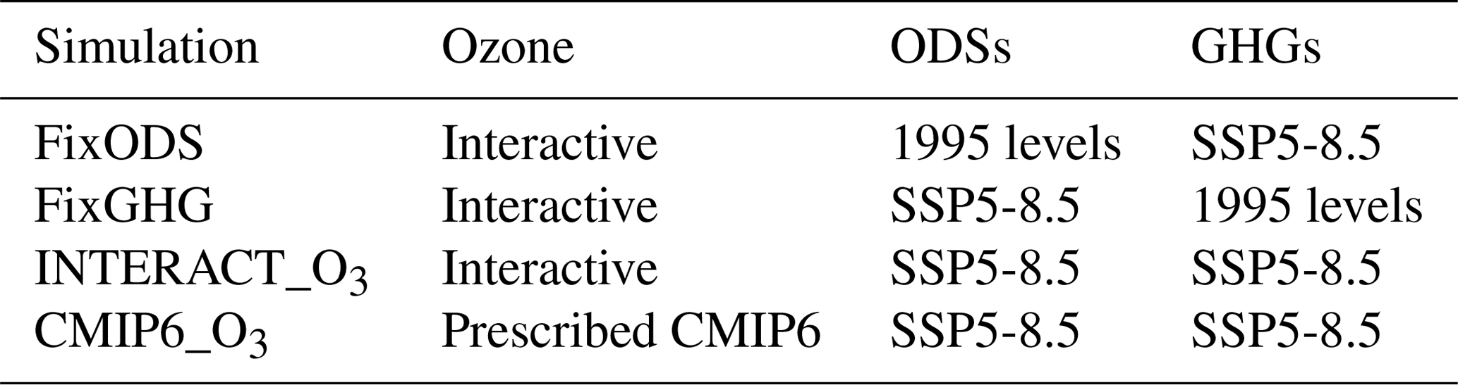
Table 2 Separation of the different effects investigated in this study. The first column gives the effect that is extracted, the second column lists the ensembles that are subtracted to extract an effect, and the third column gives the periods over which the differences are taken.

2.2 Residual circulation and wave diagnostics

We examine changes in the zonal-mean residual circulation and its drivers within the transformed Eulerian mean (TEM; Andrews et al., 1987) framework. The quasi-geostrophic Eliassen–Palm (EP) flux of wave activity, equivalent to the zonal mean of the vertical and meridional components of the Plumb flux (Plumb, 1985), is defined as

$$\begin{array}{}\text{(1)}& {\displaystyle }& {\displaystyle }{F}_{\mathit{\varphi }}=-a\cos \mathit{\varphi }\stackrel{\mathrm{‾}}{v^{\prime }{u}^{\prime }}\text{(2)}& {\displaystyle }& {\displaystyle }{F}_{\mathrm{p}}=fa\cos \mathit{\varphi }{\displaystyle \frac{\stackrel{\mathrm{‾}}{v^{\prime }{\mathit{\theta }}^{\prime }}}{\stackrel{\mathrm{‾}}{{\mathit{\theta }}_{\mathrm{p}}}}},\end{array}$$

and its divergence, $(a\cos \mathit{\varphi }{)}^{-\mathrm{1}}\mathrm{\nabla }\cdot F$, which is a measure for wave-mean flow interaction, is defined as

$$\begin{array}{}\text{(3)}& \mathrm{\nabla }\cdot F={\displaystyle \frac{\mathrm{1}}{a\cos \mathit{\varphi }}}{\displaystyle \frac{\partial \left(F_{\mathit{\varphi }}\cos \mathit{\varphi }\right)}{\partial \mathit{\varphi }}}+{\displaystyle \frac{\partial F_{\mathrm{p}}}{\partial p}}.\end{array}$$

The zonal and meridional velocity components are represented by u and v, respectively; f is the Coriolis parameter; a is the radius of the Earth; ϕ is the latitude; p is the pressure; θ is the potential temperature; and θ_p is the partial derivative of θ with respect to pressure. The overbars denote the zonal mean, and the primes denote departures from the zonal mean. The downward residual velocity, $\stackrel{\mathrm{‾}}{w^{*}}$, was calculated from the residual stream function, Ψ^*, as

$$\begin{array}{}\text{(4)}& \stackrel{\mathrm{‾}}{w^{*}}={\displaystyle \frac{gH}{pa\cos \mathit{\varphi }}}{\displaystyle \frac{\partial {\mathrm{\Psi }}^{*}}{\partial \mathit{\varphi }}},\end{array}$$

where

$$\begin{array}{}\text{(5)}& {\mathrm{\Psi }}^{*}=-{\displaystyle \frac{\cos \mathit{\varphi }}{g}}\underset{\mathrm{p}}{\overset{\mathrm{0}}{\int }}\stackrel{\mathrm{‾}}{v^{*}}(\mathit{\varphi },p)\mathrm{d}p.\end{array}$$

The meridional residual velocity is defined as

$$\begin{array}{}\text{(6)}& \stackrel{\mathrm{‾}}{v^{*}}=\stackrel{\mathrm{‾}}{v}-{\displaystyle \frac{\partial }{\partial p}}\left({\displaystyle \frac{\stackrel{\mathrm{‾}}{v^{\prime }{\mathit{\theta }}^{\prime }}}{\stackrel{\mathrm{‾}}{{\mathit{\theta }}_{\mathrm{p}}}}}\right).\end{array}$$

The scale height, H, was taken as 7000 m, and g denotes the gravitational acceleration.

2.3 Agulhas leakage calculation

As the Agulhas leakage consists of rings, eddies, and filaments, it is characterized by strong spatiotemporal variability and therefore cannot be properly measured using an Eulerian approach. Instead, the Agulhas leakage is commonly quantified using Lagrangian particle tracking (Biastoch et al., 2008, 2009; van Sebille et al., 2009; Durgadoo et al., 2013; Weijer and van Sebille, 2014; Cheng et al., 2016, 2018). Here, we follow the method of Durgadoo et al. (2013), and we use the offline ARIANE software (Blanke and Raynaud, 1997; Blanke et al., 1999) to track Lagrangian particles originating in the Agulhas Current. The virtual particles are seeded in a zonal section across the Agulhas Current at 32^∘ S over the full depth for southward velocities and are advected for a maximum period of 5 years based on the 5 d three-dimensional velocity field obtained from FOCI. Each particle has a fraction of the total instantaneous Agulhas Current volume transport assigned to it that remains constant as the particle is advected forward. An annual time series of Agulhas leakage is obtained by summing up the volume transport associated with the particles that have exited the Cape Basin through the Good Hope section, marked by the black line in Fig. 16a, within 5 years. This gives the fraction of the Agulhas Current volume transport that enters the Atlantic Ocean. The Agulhas leakage is computed for each ensemble member of FixODS, FixGHG, INTERACT_O₃, and CMIP6_O₃ before the ensemble averaging is performed. Because of the 5-year period granted for the particles to be advected, the Agulhas leakage time series ends in 2094, although the FOCI simulations were performed until 2099. Therefore, we calculated the Agulhas leakage differences between INTERACT_O₃ and FixODS or FixGHG based on the 2075–2094 period, and we estimate the total change in the Agulhas leakage by taking the difference between the 2080–2094 and 2014–2028 periods.

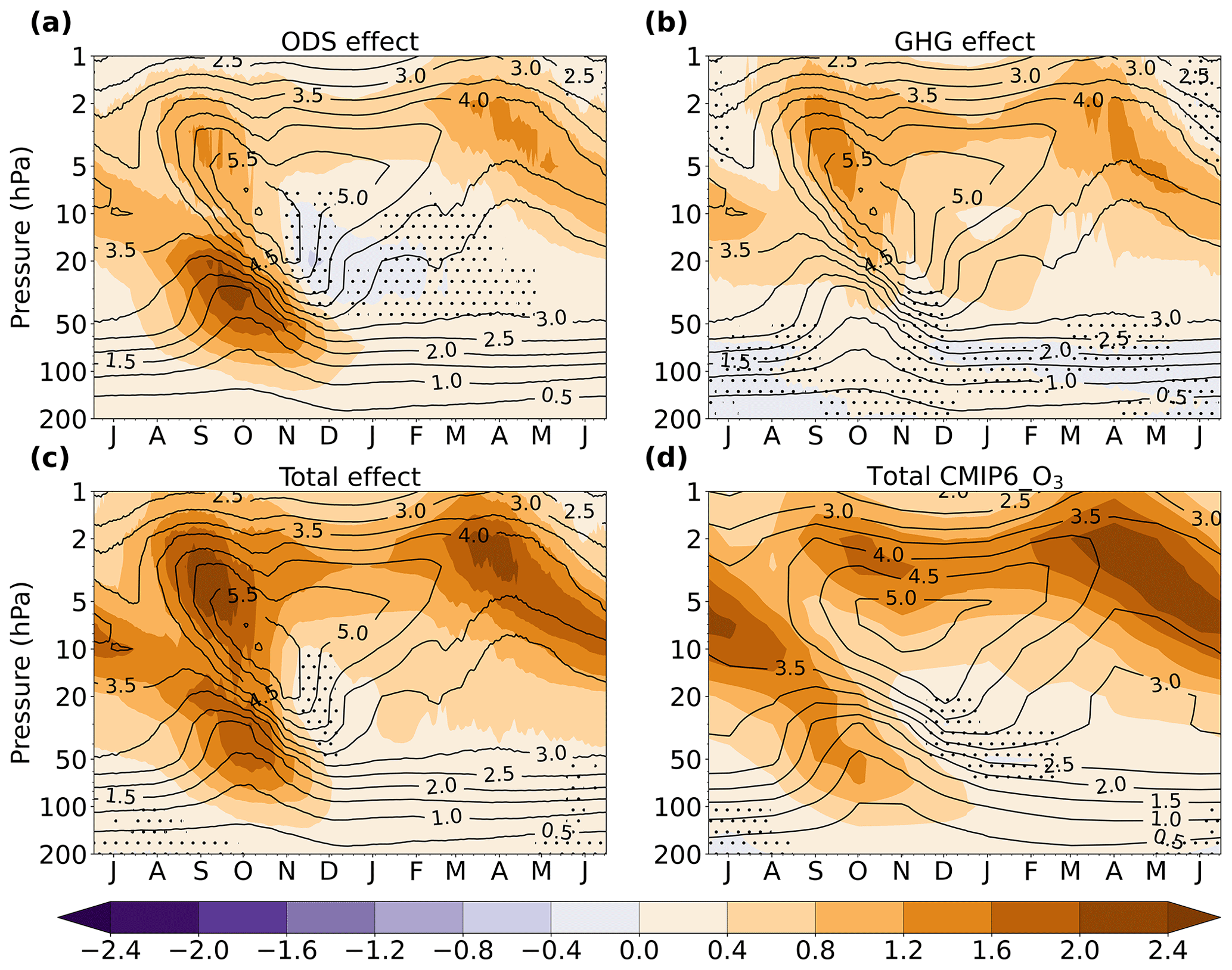
Figure 1 Changes in the polar cap (70–90^∘ S) ozone (ppmv) for each day of the year and pressure level (color shading): effect of ODSs (a), effect of GHGs (b), total effect when ozone is interactive (c), and total effect prescribed in CMIP6_O₃ (d). The contours depict the current-day (2011–2030) climatology from INTERACT_O₃ in (a)–(c) and the climatology prescribed in CMIP6_O₃ in (d). The stippling masks regions where the changes are not significant at the 95 % confidence interval based on a two-tailed t test.

3 Projected ozone recovery in FOCI

Decreasing levels of ODSs and increasing levels of GHGs both lead to changes in the stratospheric ozone. Figure 1 shows the vertical and seasonal distribution of the twenty-first-century changes in Antarctic polar cap ozone due to ODSs, GHGs, and their combined effect. Austral spring lower- and middle-stratospheric ozone levels exhibit a strong increase in response to declining ODSs (Fig. 1a), peaking in October, in agreement with results from other chemistry–climate models (CCMs) (Perlwitz et al., 2008; Son et al., 2008). This is the month during which the strongest ozone depletion occurred in FOCI in the second half of the twentieth century (Ivanciu et al., 2021). In addition, there is a significant increase in ozone throughout the whole year in the upper stratosphere and a small decrease between 30 and 10 hPa in December and January.

GHGs also influence the stratospheric ozone through their chemical, radiative, and dynamical effects (Haigh and Pyle, 1982; Rosenfield et al., 2002; Revell et al., 2012; Chiodo et al., 2018; Morgenstern et al., 2018). In the upper stratosphere, GHGs lead to an increase in ozone of similar magnitude to the ODSs effect (Fig. 1b). At these levels, GHGs have a strong cooling effect (Fig. 3b) owing to their emission of longwave (LW) radiation. This cooling slows down the temperature-dependent ozone-depleting reactions in the upper stratosphere, resulting in an increase in ozone (Haigh and Pyle, 1982; Jonsson et al., 2004; Rosenfield et al., 2002; Revell et al., 2012; Morgenstern et al., 2018). In addition, an increase in CH₄ causes an overall ozone increase, and an increase in N₂O causes an overall ozone loss through chemical processes. The influences of individual GHGs on ozone levels have been discussed in previous studies (Portmann and Solomon, 2007; Revell et al., 2012; Dhomse et al., 2018; Morgenstern et al., 2018) and are not distinguished here. We show instead the combined influence of CO₂, CH₄, and N₂O on ozone (Fig. 1b) to illustrate that the increase in GHGs drives important changes in ozone. Therefore, the GHG-induced dynamical changes discussed in the following sections include not only the direct effects of GHGs, driven by radiation changes, but also indirect effects mediated through changes in ozone. The studies by Morgenstern et al. (2014) and Chiodo and Polvani (2016) showed that these indirect effects are substantial, and they offset part of the direct GHG impacts on the tropospheric circulation.

Figure 2 Time series of polar cap (60–90^∘ S) total column ozone for October (DU) from INTERACT_O₃ in black, FixGHG in blue, and FixODS in orange. The ensemble means are depicted by thick lines and the individual members by thin lines. The dashed horizontal green lines mark the 1980 and 1960 ozone levels, computed from the ensemble mean given as the 1979–1981 and 1959–1961 averages, respectively. The time series were filtered using a 10-point boxcar filter.

Figure 1 shows that increasing GHGs and decreasing ODSs each contribute about half of the total ozone increase in the upper stratosphere (Fig. 1c). This is consistent with the findings of the latest Scientific Assessment of Ozone Depletion (World Meteorological Organization, 2018). In the lower and middle stratosphere in austral spring, the effect of declining ODSs dominates the total ozone change. GHGs also contribute a small increase in ozone at these levels in spring (Fig. 1b) by enhancing the residual circulation, which transports ozone-rich air to the polar cap, as discussed in Sect. 4.1.2.

In FOCI, the INTERACT_O₃ ensemble mean projects that the October Antarctic TCO will return to 1980s values in 2048 under the SSP5-8.5 pathway, with the spread of the individual members ranging from 2048 to 2050 (Fig. 2). This is earlier than the CCMI ensemble mean estimate of 2060, with a 1σ uncertainty of 2055–2066 (Dhomse et al., 2018), or the CCMI weighted-mean estimate of 2056, with a 95 % confidence interval of 2052–2060 (Amos et al., 2020), both of which are obtained using RCP6.0. The discrepancy to the CCMI-projected recovery date arises most likely due to higher GHG levels in SSP5-8.5, which accelerate ozone recovery. A positive trend in the October Antarctic TCO can be observed even when ODSs do not decline (FixODS ensemble), demonstrating that GHGs alone can be responsible for a substantial increase in ozone in this region (Fig. 2). In the absence of future increase in GHGs (FixGHG ensemble), the October Antarctic TCO returns to 1980 levels in FOCI only in 2067, with individual members simulating a recovery between 2066 and 2076 (Fig. 2). Our simulations therefore suggest that increasing GHGs following the SSP5-8.5 pathway accelerate Antarctic ozone recovery by at least 2 decades.

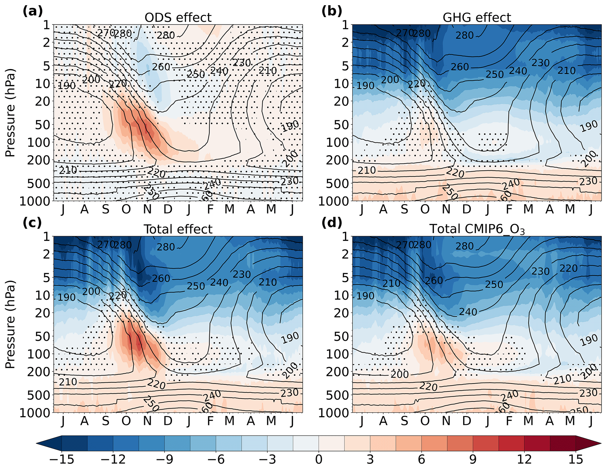
Figure 3 Changes in the polar cap (70–90^∘ S) temperature (K) for each day of the year and pressure level (color shading): effect of ozone recovery (a), effect of GHGs (b), total effect in INTERACT_O₃ (c), and total effect in CMIP6_O₃ (d). The contours depict the current-day (2011–2030) climatology from INTERACT_O₃ in (a)–(c) and from CMIP6_O₃ in (d). The stippling masks regions where the changes are not significant at the 95 % confidence interval based on a two-tailed t test.

Figure 1 offers a comparison between the total ozone change simulated by FOCI and that in the CMIP6 ozone field prescribed to the CMIP6_O₃ ensemble (Fig. 1c and d). Both fields show the recovery of the stratospheric ozone, exhibiting a maximum increase in ozone in the upper stratosphere and, during austral spring, between 100 and 20 hPa. However, there are differences in the magnitude of the ozone increase. The recovery of the ozone hole is stronger in FOCI than in the CMIP6 field. In addition, the increase in the upper stratosphere is stronger in FOCI during spring and weaker during March–June. These differences in ozone recovery between the FOCI and CMIP6 fields contribute to the different changes in temperature and atmospheric circulation in INTERACT_O₃ and CMIP6_O₃ discussed in the following sections.

4 Impacts of ozone recovery and GHG increase in the Southern Hemisphere

4.1 Atmospheric circulation changes

4.1.1 Temperature and zonal wind

Figure 3 shows the effects of ozone recovery and of increasing GHGs on the Antarctic polar cap temperature as well as their combined effects in the presence of interactive ozone (INTERACT_O₃) and of prescribed ozone (CMIP6_O₃). A significant warming occurs between 200 and 20 hPa in austral spring and summer in response to ozone recovery (Fig. 3a), in agreement with previous studies (Perlwitz et al., 2008; Son et al., 2009; Karpechko et al., 2010; McLandress et al., 2010). The warming reaches its maximum in November. Above this warming, a significant cooling occurs in November and December due to the dynamical response to ozone recovery, as discussed below. Increasing GHGs lead to a cooling of the stratosphere throughout the year, which is strongest in the upper stratosphere (Fig. 3b), in line with the findings of McLandress et al. (2010). We note that stratospheric temperature changes due to GHGs inferred from Fig. 3b include the warming caused by the GHG-driven ozone increase in the middle and upper stratosphere (Fig. 1b) and that the direct radiative effect of GHGs is likely larger. An exception to the GHG-induced stratospheric cooling occurs below 20 hPa in austral spring, when the temperature increases as a result of increasing GHGs, but this increase is not significant when the polar cap mean is considered. We show below that this is caused by a change in the PW1 in response to GHGs leading to contrasting dynamical heating over different sectors of the Southern Ocean that compensate each other in the zonal mean. In the troposphere, there is a significant warming due to GHGs throughout the entire year, reaching 4.4 K at the surface.

The combined effect of ozone recovery and GHGs (Fig. 3c and d) is dominated by the GHG-induced cooling (warming) in the stratosphere (troposphere) and by the ozone-induced warming in the lower stratosphere during spring. There is little difference between the temperature changes in the ensemble with interactive ozone, INTERACT_O₃, and the ensemble with prescribed CMIP6 ozone, CMIP6_O₃, during the months when the GHG effect dominates. In contrast, during austral spring, when the stratospheric temperature changes are dictated by changes in ozone, there is a clear difference between the two ensembles. CMIP6_O₃ simulates a spring lower-stratospheric maximum warming that is about half of that simulated by INTERACT_O₃ in the polar cap mean. In addition, the November upper-stratospheric cooling is also weaker in CMIP6_O₃ than in INTERACT_O₃.

Changes in the polar cap temperature are closely related to changes in zonal wind through the thermal wind balance. Figure 4 shows the vertical profile of the zonal-mean zonal wind changes averaged over November and December, when the largest temperature signal in the lower stratosphere occurs (Fig. 3). The ozone-induced polar cap warming is associated with a weakening of the stratospheric westerlies that extends to the troposphere and the surface (Fig. 4a). In contrast, the increasing GHGs result in a positive (westerly) wind change extending from the top of the stratosphere to the surface in the midlatitudes (Fig. 4b). The GHG effect peaks at the upper flank of the subtropical jet around 25^∘ S and occurs throughout the year, unlike the ozone effect, which occurs only during spring in the stratosphere and summer in the troposphere. The combined ozone and GHG effect consists of a weakening of the stratospheric westerlies south of 60^∘ S, where the ozone effect dominates, and a strengthening at the top of the tropospheric jet and on its poleward flank, where the GHG effect dominates (Fig. 4c and d). The stratospheric westerly wind weakening has a much lower magnitude in CMIP6_O₃ than in INTERACT_O₃, in agreement with the lower magnitude of the total spring temperature change. At the same time, the positive change in the midlatitudes is stronger and exhibits a larger latitudinal extent in CMIP6_O₃ in both the stratosphere and the troposphere as the GHG westerly effect is offset to a lesser degree by the weaker ozone easterly effect in this ensemble.

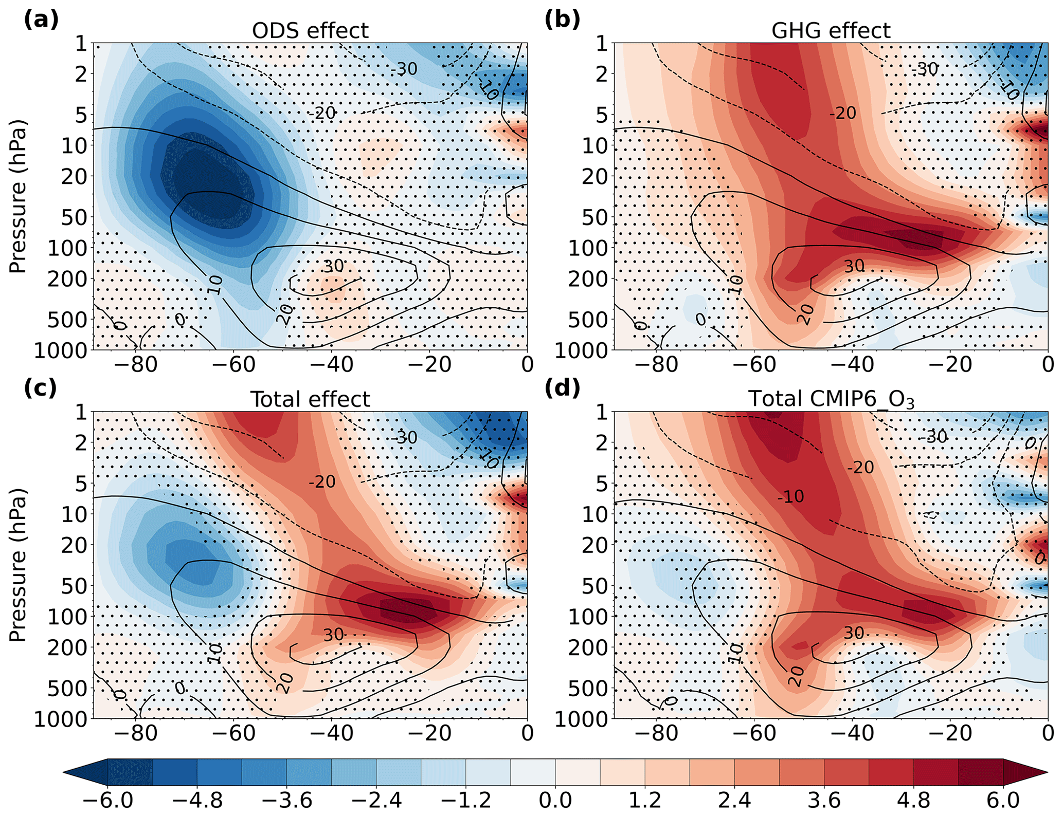
Figure 4 Changes in the November–December zonal-mean zonal wind (m s⁻¹) for each latitude and pressure level (color shading): effect of ozone recovery (a), effect of GHGs (b), total effect in INTERACT_O₃ (c), and total effect in CMIP6_O₃ (d). The contours depict the current-day (2011–2030) climatology from INTERACT_O₃ in (a)–(c) and from CMIP6_O₃ in (d). The stippling masks regions where the changes are not significant at the 95 % confidence interval based on a two-tailed t test.

The Antarctic ozone hole is not centered over the polar cap (e.g., Grytsai et al., 2007), and therefore the ozone recovery also occurs displaced from the South Pole. In addition, the dynamical effects of both ozone recovery and increasing GHGs exhibit strong zonal variations. Therefore, it is interesting to investigate the horizontal structure of the stratospheric changes. Figures 5 and 6 show maps of the October ozone and temperature changes at 50 hPa and of the zonal wind changes at 20 hPa. The region of large ozone recovery in response to declining ODS is slightly displaced towards the Atlantic sector (Fig. 5a), causing the warming response to also extend towards the Atlantic (Fig. 5b). This displacement coincides with the displacement of the ozone hole simulated by FOCI for the latter part of the twentieth century (Ivanciu et al., 2021). There is a significant ozone increase due to GHGs focused over the Pacific sector (Fig. 5d), which occurs due to changes in dynamics, as discussed below. This agrees with the zonally asymmetric ozone response to a quadrupling of CO₂ reported from four CCMs by Chiodo et al. (2018), characterized by a positive change over the Pacific and a negative one over the Indian Ocean.

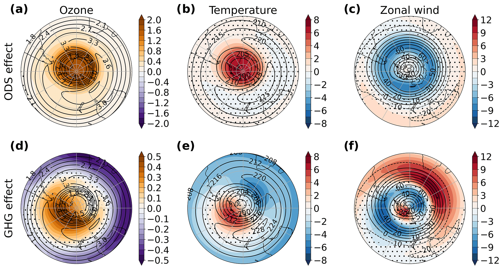
Figure 5 Changes in ozone (a, d; ppmv) and temperature (b, e; K) at 50 hPa and in zonal wind (c, f; m s⁻¹) at 20 hPa during October due to ODSs (a–c) and GHGs (d–f). The contours depict the current-day (2011–2030) climatology from INTERACT_O₃. The stippling masks regions where the changes are not significant at the 95 % confidence interval based on a two-tailed t test.

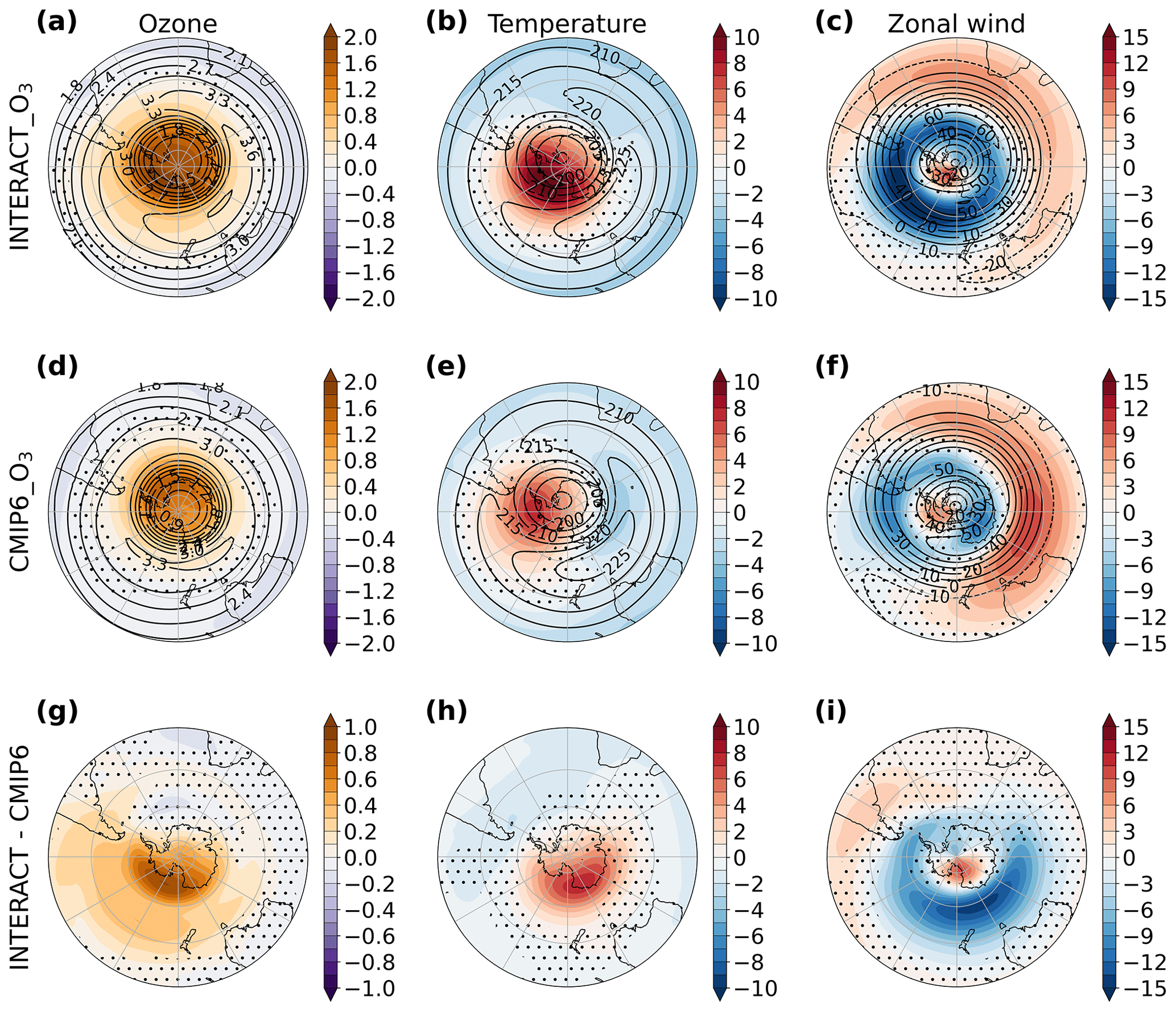
Figure 6 Changes in ozone (a, d; ppmv) and temperature (b, e; K) at 50 hPa and in zonal wind (c, f; m s⁻¹) at 20 hPa due to ODSs and GHGs combined, in INTERACT_O₃ (a–c) and in CMIP6_O₃ (d–f), and the difference between the INTERACT_O₃ and the CMIP6_O₃ changes (g–i). The stippling in (a)–(f) masks regions where the changes are not significant at the 95 % confidence interval based on a two-tailed t test, and the stippling in (g)–(i) masks regions where the difference is lower than 2σ inferred from the spread of the individual ensemble members. The contours in (a)–(f) show the current-day (2011–2030) climatologies in the respective fields.

Even more interesting is the temperature response to increasing GHGs (Fig. 5e), which is characterized by a PW1 pattern, with cooling occurring towards South Africa and warming occurring towards the Pacific, in the same region as the strongest ozone increase. To better understand these changes, Fig. 7 illustrates the temperature signature of the current-day PW1 overlaid onto its changes at the end of the century. The PW1 dominates the current-day temperature anomaly from the zonal mean, depicted by the contours in Fig. 8c and f. Comparing the current-day structure with the changes caused by GHGs (Fig. 7b), it becomes clear that the increase in GHGs leads to an eastward phase shift in the PW1. This is further confirmed by the GHG-induced changes in the dynamical heating rate depicted in Fig. 8f, which exhibit the same PW1 pattern and demonstrate that the temperature changes caused in the lower stratosphere during spring by the increase in GHGs are mediated by dynamical changes. An additional contribution is brought by the increase in the SW heating rate over the Pacific sector (Fig. 8d) caused by the dynamically induced ozone increase in response to increasing GHGs (Fig. 5). This contribution is, however, small in comparison to the contribution of the dynamical heating rate.

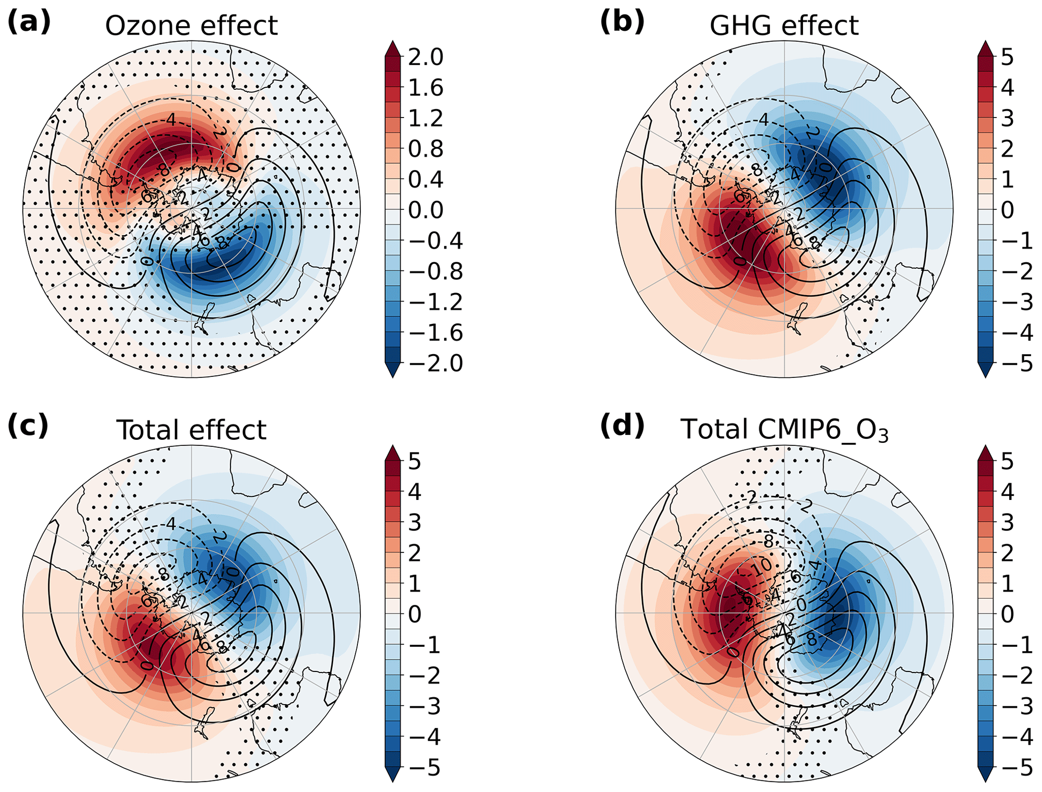
Figure 7 Changes in the temperature PW1 (K) at 50 hPa during October (color shading): effect of ozone recovery (a), effect of GHGs (b), total effect in INTERACT_O₃ (c), and total effect in CMIP6_O₃ (d). The contours depict the current-day (2011–2030) PW1 climatology from INTERACT_O₃ in (a)–(c) and from CMIP6_O₃ in (d). The stippling masks regions where the changes are not significant at the 95 % confidence interval based on a two-tailed t test.

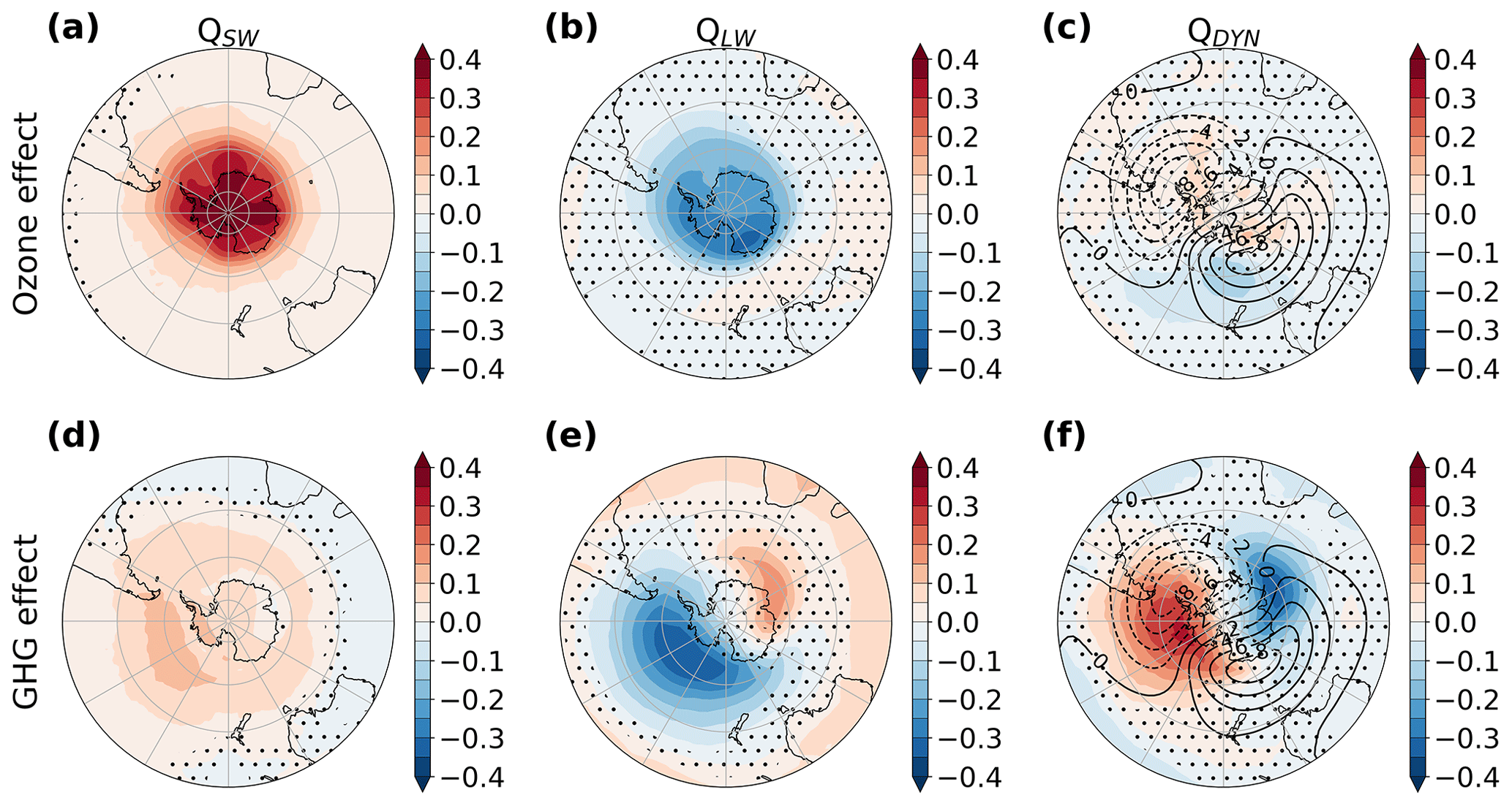
Figure 8 Changes in the SW (a, d), LW (b, e), and dynamical (c, f) heating rates (K d⁻¹) at 50 hPa during October due to ozone recovery (a–c) and GHGs (d–f). The contours in panels (c) and (f) depict the current-day (2011–2030) climatology of the temperature deviations from the zonal mean from INTERACT_O₃. The stippling masks regions where the changes are not significant at the 95 % confidence interval based on a two-tailed t test.

Ozone recovery also alters the PW1 (Fig. 7a), dampening its amplitude and slightly altering its phase, but its impact is smaller than that of the GHGs. Unlike the GHG effect, the ozone effect is radiative in nature. The increase in ozone results in more SW radiation being absorbed, warming the lower stratosphere in spring, as shown by the change in the SW heating rate (Fig. 8a). The change in the PW1 depicted in Fig. 7a is a consequence of the fact that the polar vortex, the ozone hole, and consequently its recovery are not centered on the South Pole, being displaced towards the Atlantic Ocean (Figs. 5 and 6).

We note that the magnitude of the total GHG-induced October warming reaches 7 K, only 1 K lower than the maximum warming associated with ozone recovery of 8 K, while the maximum GHG-induced cooling reaches −6 K (Fig. 5b and e). This indicates that the increase in GHGs results in important temperature changes in the lower stratosphere during spring, substantially contributing to the total temperature change in Fig. 6b. However, although the temperature changes resulting from ozone recovery and increasing GHGs have similar magnitudes, the mechanisms behind these changes are different. As shown above, while the temperature changes caused by ozone recovery (Fig. 5b) result primarily from radiative processes, the changes occurring in the springtime lower stratosphere due to GHGs (Fig. 5e) are a result of dynamical processes. The GHG-induced springtime lower-stratospheric temperature changes are largely underestimated if zonally averaged fields are investigated (Fig. 3b) as the PW1 anomalies cancel out to a large degree.

The total October lower-stratospheric temperature change (Fig. 6b) illustrates the combination of the ozone and GHG effects well. The ozone-induced warming persists over Antarctica, but it is extended towards the Pacific by the superposition of the GHG-induced warming. The cooling due to GHGs dominates over the Southern Ocean towards South Africa and at lower latitudes. Consistent with these changes, the PW1 in INTERACT_O₃ exhibits a phase shift akin to the GHG effect, but of smaller amplitude (Fig. 7c).

The PW1 pattern of the spring temperature response to GHGs is associated with zonal wind changes of opposite sign in the Eastern Hemisphere and Western Hemisphere (Fig. 5f). The Pacific sector is characterized by a weakening of the polar night jet on its equatorward flank and a strengthening on its poleward flank, while the opposite occurs over the Atlantic and Indian sectors. This implies a shift in the polar vortex towards South Africa in austral spring driven by increasing GHGs. In contrast, ozone recovery leads to a circumpolar weakening of the polar night jet (Fig. 5c). The total stratospheric zonal wind change in October (Fig. 6c) consists of a weakening of the polar night jet, which peaks over the Pacific sector, where the GHG effect reinforces the weakening due to ozone recovery. The maximum weakening in this region reaches 16.5 m s⁻¹, or 41 % of the current-day October climatological strength of the polar vortex. At midlatitudes over the Atlantic and Indian sectors the GHG effect dominates, and the outer flank of the polar vortex strengthens, while the easterlies weaken. The maps showing the temperature and zonal wind changes in Figs. 5 and 6 demonstrate that important GHG-induced changes are missed if only changes in zonal-mean fields are investigated.

The total zonal wind change in the CMIP6_O₃ ensemble (Fig. 6f) resembles that caused by GHGs, indicating that the ozone effect is weaker in this ensemble. The magnitude of the polar vortex weakening is significantly larger in INTERACT_O₃ than in CMIP6_O₃ over the Pacific sector (Fig. 6i). At the same time, the strengthening over the Indian sector is weaker in INTERACT_O₃ than in CMIP6_O₃. These differences arise from the different temperature response in the two ensembles (Fig. 6b, e, and h). The total temperature change in CMIP6_O₃ retains more of the PW1 structure caused by GHGs. This suggests that the increase in GHGs plays a more dominant role in driving the temperature changes in this ensemble. The region of increasing temperature is shifted eastward, and the maximum warming is weaker by about 3 K in CMIP6_O₃ compared to INTERACT_O₃. The eastwards shift is even more noticeable in the changes experienced by the PW1 in CMIP6_O₃ compared to INTERACT_O₃ (Fig. 7c and d).

These differences in the temperature response can be partly explained by the patterns of ozone recovery in INTERACT_O₃ and prescribed to CMIP6_O₃ (Fig. 6a and d). There is a stronger increase in ozone over the Pacific sector in INTERACT_O₃ (Fig. 6g), with ozone recovery peaking between the Antarctic Peninsula and the Ross Sea in this ensemble (Fig. 6a). In contrast, ozone recovery peaks over the Weddell Sea in the CMIP6 field (Fig. 6b). The different ozone recovery patterns cause the temperature response to ozone recovery to offset and reinforce the response to increasing GHGs in different regions in the two ensembles. At the same time, the smaller ozone increase in CMIP6_O₃ leads to an overall weaker response to ozone recovery and to GHGs playing a more important role in this ensemble. We also note that the shape and the magnitude of the current-day ozone hole differ between INTERACT_O₃ and CMIP6_O₃ (contours in Fig. 6a and d), with the ozone hole in CMIP6_O₃ being displaced towards South Africa and the ozone hole in INTERACT_O₃ being displaced towards South America.

The total change in the SW heating rate (Fig. 9a and d) illustrates the effect of the differences in ozone recovery on the temperature change in INTERACT_O₃ and CMIP6_O₃. The effect of ozone recovery dominates the total change in the SW heating rate (Fig. 9a), but there is also a small contribution arising from the GHG-driven spring increase in ozone (Fig. 8d). In agreement with the stronger ozone increase in INTERACT_O₃, there is a stronger SW warming over Antarctica and extending to the South Pacific in this ensemble compared to CMIP6_O₃ (Fig. 9a, d, and g). This contributes to the larger temperature increase simulated by INTERACT_O₃ (Fig. 6b). Interestingly, the region over the Pacific sector where ozone levels (Fig. 6g) and SW heating (Fig. 9g) are higher in INTERACT_O₃ compared to CMIP6_O₃ coincides with the region of GHG-induced ozone increase (Fig. 5d). The effect of GHGs on ozone represents a dynamical feedback that cannot be simulated in CMIP6_O₃ because the ozone field is prescribed and therefore cannot react to changes in dynamics. Although this GHG effect is captured in the two CCMs that produced the CMIP6 ozone field prescribed in CMIP6_O₃, and although this ozone field is consistent with the SSP5-8.5 scenario used here, intermodel differences in simulating the ozone response to increasing GHGs and declining ODSs lead to inconsistencies between ozone and dynamical changes when the ozone field obtained from other models is prescribed. This is emphasized by the weak ozone and SW heating rate changes in CMIP6_O₃ in the region where the dynamical increase in ozone driven by GHGs occurs in FOCI.

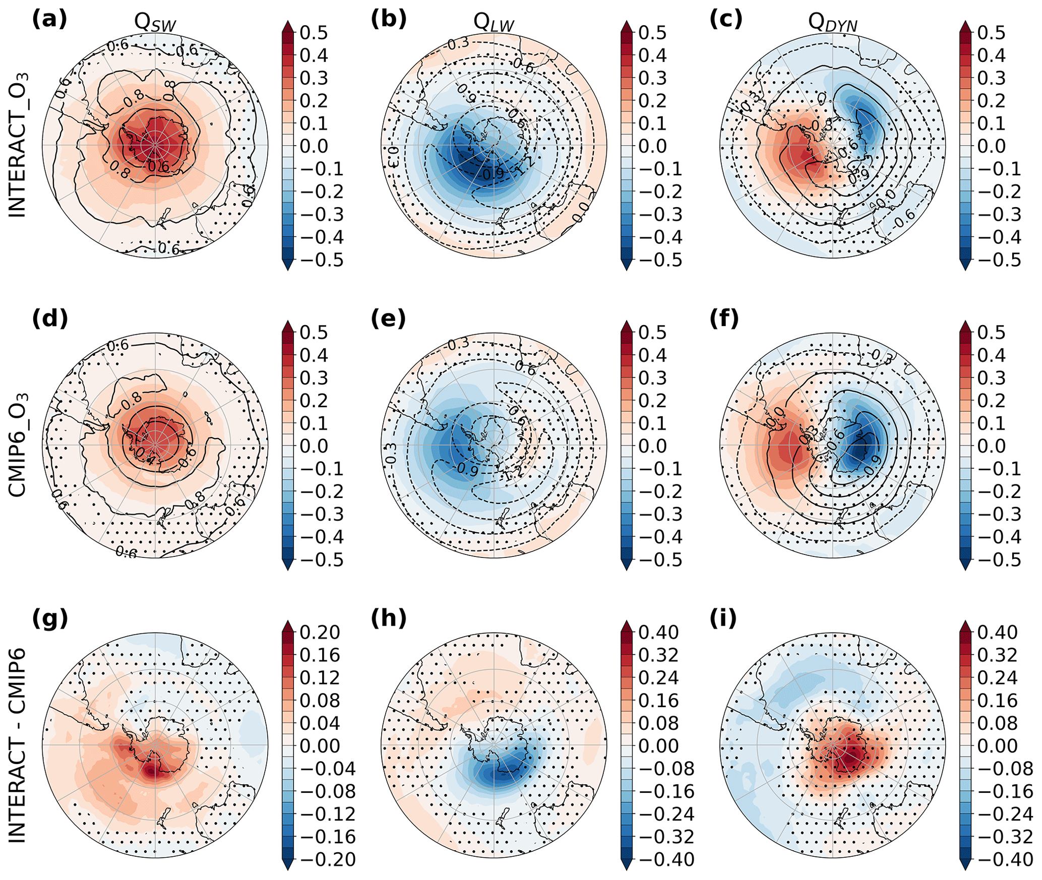
Figure 9 Changes in the SW (a, d), LW (b, e), and dynamical (c, f) heating rate (K d⁻¹) at 50 hPa during October due to ozone recovery and GHGs combined, in INTERACT_O₃ (a–c) and CMIP6_O₃ (d–f), and the difference between the INTERACT_O₃ and the CMIP6_O₃ changes (g–i). The stippling in (a)–(f) masks regions where the changes are not significant at the 95 % confidence interval based on a two-tailed t test, and the stippling in (g)–(i) masks regions where the difference is lower than 2σ inferred from the spread of the individual ensemble members. The contours in (a)–(f) show the current-day (2011–2030) climatologies in the respective fields.

The pattern of changes in the dynamical heating rate in INTERACT_O₃ is driven by the dynamical response to increasing GHGs (Fig. 8f). The change in the dynamical heating rate due to ozone recovery is weak in October at 50 hPa (Fig. 8c), but it becomes stronger in November, acting to cool the polar cap (Fig. S4l). The region of dynamical warming is larger, and the dynamical cooling is stronger in CMIP6_O₃ (Fig. 9f) than in INTERACT_O₃ (Fig. 9c). These differences in the dynamical heating rate originate from differences in wave activity and in the residual circulation, which are discussed in the following section. The LW heating rate changes act to dampen the warming due to SW and dynamical heating changes in all simulations (Figs. 8b, e and 9b, e).

In summary, ozone recovery during the twenty-first century reverses the effects of ozone depletion. It leads to a springtime warming of the polar cap in the lower stratosphere and an associated weakening of the westerly winds that extends to the surface in austral summer. In contrast, increasing GHGs lead to a cooling of the stratosphere throughout most of the year, an acceleration of the subtropical jet, and enhanced westerly winds throughout the stratosphere. These results are in good agreement with the findings of previous studies (Perlwitz et al., 2008; Karpechko et al., 2010; McLandress et al., 2010; Polvani et al., 2011a). A significant exception to the otherwise rather zonally uniform changes occurs in austral spring, when a dynamical response to increasing GHGs results in contrasting temperature and zonal wind changes over the Pacific and Indo-Atlantic sectors that offset each other in the zonal mean and are not detectable if only zonal-mean fields are investigated. The importance of these GHG-driven changes, which are reported here for the first time, is emphasized by their magnitude, which is similar to the magnitude of the changes due to ozone recovery. In the months and regions where the ozone effect is important, the combined ozone and GHG effect is stronger in the stratosphere in the ensemble with interactive ozone chemistry than in the ensemble with prescribed CMIP6 ozone as the ozone effect is stronger in the former ensemble. This demonstrates the importance of the ozone field in setting the magnitude of the temperature and zonal wind changes during the twenty-first century.

Figure 10 Changes in the SH downward mass flux (a, b), NH downward mass flux (c, d), and tropical upward mass flux (e, f) at 50 hPa for each month (10⁹ kg s⁻¹). The changes due to ozone recovery are shown in blue, the changes due to GHGs are shown in orange (a, c, e), the total changes in INTERACT_O₃ are shown in black, and the total changes in CMIP6_O₃ are shown in gray (b, d, f). The error bars give the 95 % confidence interval based on a two-tailed t test. Differences between ensemble means are depicted by filled circles, and differences between individual simulations are depicted by hollow circles.

4.1.2 The residual circulation and wave activity

Although the BDC comprises both the mean meridional residual circulation and two-way mixing processes, here we only investigate the contributions of ozone recovery and increasing GHGs to the twenty-first-century changes in the residual circulation. The reduction in ODSs could also theoretically lead to changes in the BDC through the radiative effects of the ODSs. However Abalos et al. (2019) showed that trends in the BDC due to ODSs are mainly explained by ozone changes. We therefore attribute the ODS-induced residual circulation changes in our simulations to ozone recovery. As a first measure of the changes in the strength of the residual circulation, we analyze the tropical upward mass flux and the extratropical downward mass flux in each hemisphere, shown in Fig. 10 at the 50 hPa level for each month. In both hemispheres, the impact of increasing GHGs is a clear strengthening of the downward mass flux and hence of the BDC, peaking between mid-fall and mid-spring and ceasing in late spring and early summer. For the Northern Hemisphere (NH), the peak GHG-induced strengthening of the BDC in winter agrees with the results of previous studies (e.g., Shepherd and McLandress, 2011; Chrysanthou et al., 2020). For the SH, our results are at odds with those of Chrysanthou et al. (2020), who reported a peak strengthening of the BDC in austral summer in response to a quadrupling of CO₂ in an atmospheric model with prescribed preindustrial ozone. We note that the GHG-induced strengthening of the residual mean stream function is confined north of 55^∘ S in austral winter, unlike in summer, when it reaches the polar region. The magnitude of the strengthening during winter is, however, much larger than that during summer. An important exception to the GHG-induced strengthening occurs in November in the SH, when GHGs lead to a weakening of the mass flux in the lower stratosphere. The upward tropical mass flux is enhanced by increasing GHGs throughout the year, driven from the NH between November and February, in agreement with the simulations by Oberländer et al. (2013); from the SH between May and July; and from both hemispheres to different extents for the rest of the year. In contrast, ozone recovery weakens the BDC, which is consistent with previous studies (Oman et al., 2009; Lin and Fu, 2013; Oberländer et al., 2013; Polvani et al., 2018, 2019). The ozone effect is strong in the lower stratosphere only in November–December in the SH and April–May in the NH. The largest impact occurs in the SH in November, when the recovery of the Antarctic ozone hole takes place. This is also the only month when the tropical mass flux is significantly affected by ozone recovery.

Throughout most of the year, the total change in the BDC during the twenty-first century follows the change due to increasing GHGs, and the BDC strengthens. In November and December, however, the BDC in the SH weakens, driven by both ozone recovery and increasing GHGs in November and by ozone recovery alone in December. The weakening in the SH offsets the strengthening in the NH during November, leading to an insignificant change in the tropical mass flux. The change in the residual mean stream function shown for November in Fig. S1 in the Supplement reveals that while ozone recovery weakens the BDC throughout the depth of the stratosphere, the increase in GHGs only weakens the lower branch.

Figure 11 Changes in the polar cap (70–90^∘ S) vertical residual velocity (in mm s⁻¹) for each month and pressure level (color shading): effect of ozone recovery (a), effect of GHGs (b), total effect in INTERACT_O₃ (c), and total effect in CMIP6_O₃ (d). The contours depict the current-day (2011–2030) climatology from INTERACT_O₃ in (a)–(c) and from CMIP6_O₃ in (d). The stippling masks regions where the changes are not significant at the 95 % confidence interval based on a two-tailed t test.

The 2 months during which ozone recovery influences the BDC are also the 2 months during which all three members of the INTERACT_O₃ ensemble simulate a stronger weakening than all three members of the CMIP6_O₃ ensemble (hollow circles in Fig. 10b). This once again points to the fact that the effects of ozone recovery are weaker when the CMIP6 ozone field is prescribed. A similar behavior occurs in May in the NH, although the ozone recovery has a weaker effect there. In addition, the November BDC weakening is confined below 20 hPa in CMIP6_O₃, exhibiting a structure more similar to that of the GHG effect, while the weakening in INTERACT_O₃ extends to the upper stratosphere, in accordance with the ozone effect (Fig. S1).

The changes in the residual circulation described above are driven by changes in planetary wave activity in response to ozone recovery and increasing GHGs. In order to better understand the link between the changes in the residual circulation and changes in wave activity, we show in Fig. 11 the changes in the polar cap vertical residual velocity, in Fig. 12 the changes in the divergence of the EP flux, and in Fig. S2 the change in the eddy heat flux for each calendar month. As these diagnostics only offer a zonal-mean view of the simulated changes, we additionally make use of the three-dimensional Plumb flux of wave activity (Plumb, 1985) to obtain the spatial pattern of the changes (Figs. S4 and S5). When zonal averages are considered, the vertical and meridional components of the Plumb flux reduce to the EP flux. Therefore, the zonal-mean eddy heat flux (Fig. S2) is equivalent to the zonal mean of the vertical component of the Plumb flux (Figs. S4 and S5), with negative eddy heat flux values indicating upward wave activity propagation.

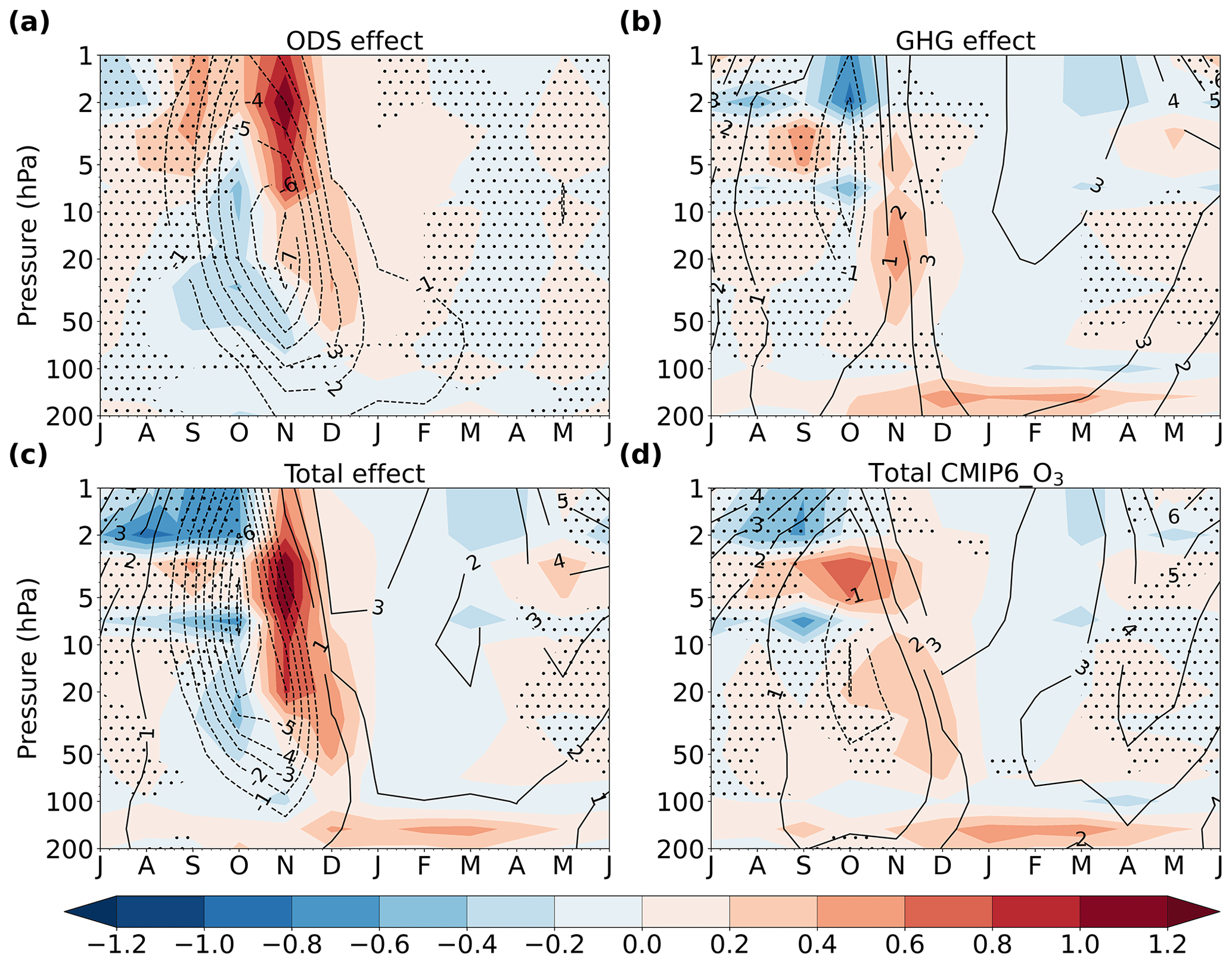
Figure 12 Changes in the divergence of the EP flux averaged over 45–80^∘ S (m s⁻¹ d⁻¹) for each month and pressure level (color shading): effect of ozone recovery (a), effect of GHGs (b), total effect in INTERACT_O₃ (c), and total effect in CMIP6_O₃ (d). The contours depict the corresponding changes in the zonal-mean wind averaged over 45–80^∘ S (m s⁻¹). The stippling masks regions where the changes are not significant at the 95 % confidence interval based on a two-tailed t test.

In agreement with the ozone-induced weakening of the mass flux (Fig. 10a), the downwelling over the polar cap is considerably reduced in November throughout the stratosphere due to ozone recovery (Fig. 11a), dynamically cooling the polar cap (Fig. S4k and l) and offsetting a part of the radiative warming effect of ozone recovery. This reduction is accompanied by an anomalous divergence of the EP flux (Fig. 12a) and a positive change in the eddy heat flux (Fig. S2a), indicating reduced wave activity propagation. Separating the divergence of the EP flux into contributions from individual zonal wavenumbers reveals that the ozone-induced changes in the residual circulation are primarily mediated through changes in the propagation of the PW1 (Fig. S3a). We showed in Sect. 4.1.1 that ozone recovery reduces the amplitude of the PW1. The weakening of the planetary wave activity flux and the associated weakening of the downwelling are initiated in the upper stratosphere in October over the Atlantic sector and Drake Passage (Fig. S4a) and become more pronounced and circumpolar and extend to the lower stratosphere in November, persisting in the lower stratosphere until February, but with a much lower magnitude (Figs. S4c and d, 11a, and 12a). The changes in the wave activity flux due to ozone recovery are linked to changes in the polar night jet. The region of zero zonal wind velocity represents the critical line for Rossby wave propagation (Dickinson, 1968). As the jet is decelerated in October in response to the ozone-induced polar cap warming (Fig. 5 and contours in Fig. 12), the critical line for Rossby wave propagation migrates poleward, inhibiting wave propagation. This mechanism is analogous to that demonstrated to be responsible for mediating the effect of increasing GHGs on the BDC in the subtropical lower stratosphere by Shepherd and McLandress (2011). Since the polar vortex in FOCI is displaced towards South America (contours in Fig. 6c), the inhibition of wave propagation is initiated in this region (Fig. S4a). The effect then extends around the Antarctic continent and propagates downward in the following month (Fig. S4c and d) as the polar night jet continues to weaken, and the breakdown of the polar vortex is accelerated by ozone recovery. In summer, the height of the critical line for Rossby wave propagation in the lower stratosphere is decreased in response to ozone recovery (Fig. 12), explaining the weak deceleration of the residual circulation in this season.

We additionally note that ozone recovery leads to anomalous convergence between 50 and 7 hPa in October (Fig. 12a) and a weak but significant strengthening of the lower-stratospheric downwelling (Fig. 11a). This corroborates the results of McLandress et al. (2010), who found an increase in the polar cap downwelling in the lower stratosphere in spring driven by enhanced EP flux convergence due to ozone recovery, changing sign in summer. In our simulations, however, the change in sign occurs already in November. This offers a possible explanation as to why previous studies that looked at seasonally averaged changes did not find an impact of ozone recovery on the BDC in spring (Polvani et al., 2018; Lin and Fu, 2013). The strengthening of the polar downwelling in the lower stratosphere during October agrees with the changes inferred from the Plumb flux and from the dynamical heating rate (Fig. S4a and i): wave propagation is inhibited in the upper stratosphere, and wave breaking occurs at lower levels, leading to a reduction in the downwelling in the upper stratosphere, resulting in dynamical cooling and an enhancement of the downwelling in the lower stratosphere (Fig. 11a).

The increase in GHGs also exerts the largest influence on the SH polar cap downwelling in austral spring (Fig. 11b). The relatively small impact of GHGs on the polar downwelling during the rest of the year might seem at odds with the peak GHG-induced increase in the downward mass flux between April and October (Fig. 10a). This discrepancy is explained by seasonal differences in the latitude range at which the residual circulation is affected by the GHG increase. During winter, although the GHG effect on the residual circulation has the largest magnitude, it is restricted to the low latitudes and midlatitudes as the propagation of wave activity is enhanced towards the Equator (not shown). During spring, the GHG effect extends to the polar latitudes, affecting the polar downwelling, although its overall magnitude is weaker. McLandress et al. (2010) also showed that important changes in the SH downward mass flux caused by increasing GHGs occur outside of the polar cap. Therefore, the seasonality of the polar downwelling and of the SH total downward mass flux magnitudes is not directly comparable. The effects of ozone recovery on the polar cap downwelling and on the total SH downward mass flux are in better agreement as the ozone-induced residual circulation changes are driven from the polar region.

Figure 11b shows that GHGs strengthen the downwelling above 20 hPa in October. This strengthening is related to enhanced planetary wave propagation (Fig. S2b) and wave breaking (Fig. 12b) in the upper stratosphere, primarily associated with the PW1 (Fig. S3b). The changes in the three-dimensional flux of wave activity (Fig. S4e and f) show that, in fact, the flux of wave activity is enhanced over the Indian Ocean sector and diminished over the Pacific and Atlantic sectors. These changes persist throughout the depth of the stratosphere and indicate that increasing GHGs enable planetary waves to propagate higher into the stratosphere and mesosphere over the Indian Ocean during spring. This results in reduced (enhanced) wave breaking in the middle (upper) stratosphere, which in turn drives a weakening (strengthening) of the downwelling in the middle (upper) stratosphere. Over the Pacific sector, the propagation of wave activity is inhibited by increasing GHGs. Consequently, planetary waves break at lower levels, and the wave drag is enhanced in the middle stratosphere and weakened above, driving stronger downwelling in the lower to middle stratosphere and weaker downwelling in the upper stratosphere. The changes over the Indian Ocean sector have a larger magnitude than those occurring over the Pacific sector and therefore dominate in the zonal mean. As such, the enhanced upward eddy heat flux (Fig. S2b), as well as the enhanced wave drag (Fig. 12b) during October in the upper stratosphere, is consistent with the changes inferred from the Plumb flux. In November, the changes over the Atlantic and Pacific sectors become dominant (Fig. S4h), consistent with the weakened eddy heat flux (Fig. S2b) as well as with the weakened wave breaking (Fig. 12b) in the middle stratosphere that results in the reduced downwelling (Fig. 11b). In fact, as shown in Fig. S1b in the Supplement, the entire lower branch of the BDC in the SH weakens in November, in agreement with the reduction in the downward mass flux (Fig. 10a).

When the combined effect of ozone recovery and increasing GHGs is considered, the weakening of the wave drag and downwelling due to ozone recovery largely offsets the strengthening due to GHGs during October in the upper stratosphere, while in the lower stratosphere the ozone-induced strengthening appears to dominate in INTERACT_O₃ (Figs. 11c and 12c). CMIP6_O₃, however, exhibits a weakening of the downwelling in the lower stratosphere during October (Fig. 11d). During November, INTERACT_O₃ exhibits a strong wave drag reduction extending from 50 hPa to the stratopause and a weakening of the downwelling between 200 and 2 hPa. While the changes in CMIP6_O₃ agree in sign with those in INTERACT_O₃ in November, the magnitude of the changes is weaker in the former ensemble, and, in addition, the changes do not extend as high up as in INTERACT_O₃ (Figs. 11c, d and 12c, d). The weaker magnitude of the changes in CMIP6_O₃ is consistent with the weaker ozone increase in the CMIP6 field. At the same time, the different timing and vertical distribution of the weakening in polar downwelling are explained by differences in the patterns of change in the propagation of planetary waves (Figs. 7c, d and S5). Thus, both the magnitude and the different spatial pattern of the ozone increase in CMIP6_O₃ compared to INTERACT_O₃ contribute to the differences in the dynamical changes between the two ensembles.

In summary, the BDC in the SH strengthens throughout most of the year, driven by the increase in GHGs, but weakens in November and December, driven by both ozone recovery and increasing GHGs in November and by ozone recovery alone in December. An interesting result of our analysis is that, during November, unlike during the rest of the year, the increase in GHGs weakens the BDC in the lower stratosphere. During the months in which ozone recovery significantly affects the BDC, the magnitude of the change in the ensemble with interactive ozone is significantly larger than in the ensemble with prescribed CMIP6 ozone. Furthermore, while the changes in the former ensemble occur throughout the depth of the stratosphere, the changes in the latter ensemble are only significant up to the middle stratosphere. This shows that the effect of ozone recovery on the BDC is weaker when the CMIP6 ozone field is prescribed.

Figure 13 Changes in annual mean sea level pressure (a, d; hPa), surface zonal wind (b, e; m s⁻¹), and wind stress curl (c, f; 10⁻⁷ N m⁻³) due to ozone recovery (a–c) and GHGs (d–f). The stippling masks regions where the changes are not significant at the 95 % confidence interval based on a two-tailed t test. The contour in (c) and (f) marks the location of zero-wind-stress curl.

4.1.3 Surface impacts

We now turn our attention to the projected twenty-first-century changes in the surface circulation. As shown in Sect. 4.1.1, the weakening of the stratospheric westerlies due to ozone recovery extends to the surface in November and the austral summer. Figure 13 shows maps of annual changes in the mean sea level pressure (SLP), surface zonal wind, and the associated wind stress curl, in response to ozone recovery and increasing GHGs, separately. We chose to examine the changes occurring over the entire year rather than seasonal subsets as they are the most relevant for the long-term trends in the ocean circulation. For completion, we show additional maps of zonal wind changes during November–January and June–August in Fig. S6. Although occurring during a single season, the ozone effect is still significant in the annual mean and represents a weakening of about 4 % of the current-day annual mean westerlies in the latitude band between 45 and 60^∘ S. In the November–January average, the weakening is larger, reaching 8 %. The change towards more easterly velocities occurs on the poleward flank of the climatological westerlies (contours in Fig. 14b) and implies an equatorward shift in their position. As expected, ozone recovery reverses the strengthening and poleward shift in the westerlies caused in the past by the formation of the Antarctic ozone hole, consistent with previous findings (Perlwitz et al., 2008; McLandress et al., 2011). This can also be seen in the effect of ozone recovery on SLP (Fig. 13a), which exhibits a strong increase over the Antarctic continent and decreases at midlatitudes, signaling that the SAM shifts more towards its negative phase. This is confirmed by the negative change in the SAM index shown in Fig. 15a.

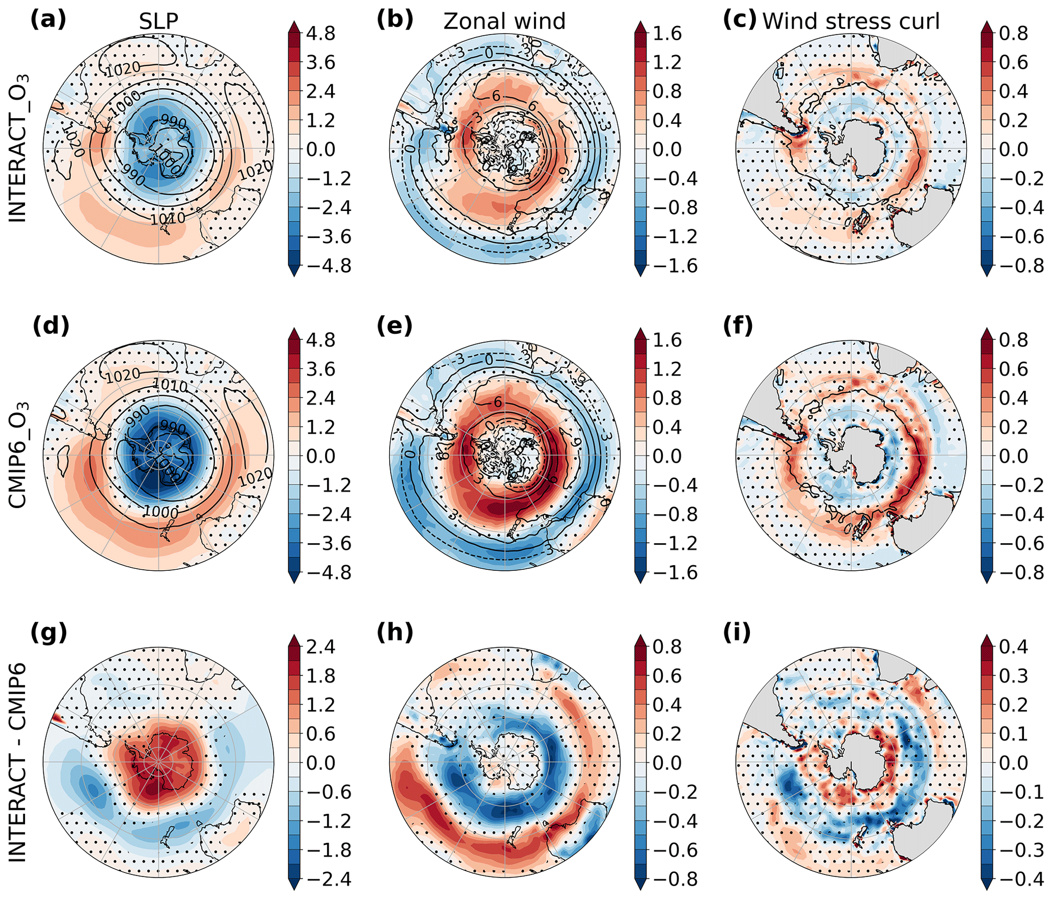
Figure 14 Changes in annual mean sea level pressure (a, d; hPa), surface zonal wind (b, e; m s⁻¹), and wind stress curl (c, f; 10⁻⁷ N m⁻³) due to ozone recovery and GHGs combined, in INTERACT_O₃ (a–c) and CMIP6_O₃ (d–f), and the difference between the INTERACT_O₃ and the CMIP6_O₃ changes (g–i). The stippling in (a)–(f) masks regions where the changes are not significant at the 95 % confidence interval based on a two-tailed t test, and the stippling in (g)–(i) masks regions where the difference is lower than 2σ inferred from the spread of the individual ensemble members. The contour in (c) and (f) marks the location of zero-wind-stress curl, while contours in (a), (b), (d), and (e) show the current-day (2011–2030) climatologies in the respective fields.

Figure 15 Changes in the annual mean SAM index calculated following the definition of Gong and Wang (1999) as the difference in the normalized zonal-mean SLP between 40 and 65^∘ S (a); surface westerly jet position computed as the latitude of the maximum in the zonal-mean zonal wind between 30 and 65^∘ S (b; ^∘ of latitude, positive northward); surface westerly wind strength averaged between 45 and 60^∘ S (c; m s⁻¹); ACC transport (d; Sv) in the Drake Passage, computed as the difference in the barotropic stream function between the Antarctic Peninsula and South America (circles), and south of Africa, computed as the maximum in the barotropic stream function between 20 and 30^∘ E (triangles); wind stress curl averaged between 40 and 55^∘ S and 30 and 120^∘ E (e; 10⁻⁷ N m⁻³); Agulhas leakage transport (f; Sv); Agulhas Current transport (g; Sv); and the zonal wind at 32^∘ S averaged between 30 and 120^∘ E (h; m s⁻¹). Filled symbols depict the change in the ensemble mean, and hollow symbols depict the change in the individual members due to ozone recovery (blue) increasing GHGs (orange), combined forcing in INTERACT_O₃ (black), and combined forcing in CMIP6_O₃ (gray). The error bars denote the 95 % confidence interval based on a two-tailed t test.

Increasing GHGs, in contrast, continue the past trend towards a more positive SAM (Figs. 13d and 15a) and strengthened surface westerlies that shift poleward (Figs. 13e and 15b, c). The magnitude of the GHG effect is much larger than that of the ozone effect on the westerlies in the annual mean, leading to a strengthening of 17 % in the mean over the latitude band between 45 and 60^∘ S. As a consequence, when both effects are considered together (Fig. 14a), the GHG effect dominates, and the westerlies continue to strengthen and shift poleward during the twenty-first century (Fig. 15b and c), accompanied by a shift toward the positive phase of the SAM (Figs. 14a and 15a). There are marked differences between INTERACT_O₃ and CMIP6_O₃ in the magnitude of the total SAM change and in the magnitude of the total westerly wind change (Figs. 14 and 15). Significant differences between the two ensembles occur particularly over the Indian and Pacific oceans for both zonal wind and SLP and additionally over the entire Antarctic continent for SLP, with changes in both signs being stronger in CMIP6_O₃ (Fig. 14). Averaged over 45 and 60^∘ S, the westerlies strengthen by 9 % compared to the current day in INTERACT_O₃, while they strengthen by 16 % in CMIP6_O₃. Given that the difference between INTERACT_O₃ and CMIP6_O₃ lies in the treatment of ozone chemistry, the stronger changes in CMIP6_O₃ in the direction driven by GHGs show that the ozone effect is much weaker in CMIP6_O₃. This is consistent with the results presented in the previous sections for the stratosphere, where the impact of ozone recovery is also weaker in this ensemble.

We stress that the dominance of the GHG effect over the effect of ozone recovery on the surface winds is strongly dependent on the scenario used for GHGs. Here, we use SSP5-8.5, which is characterized by high GHG emissions throughout the twenty-first century. CMIP6 models project that, for the “sustainability” scenario SSP1-2.6, the ozone effect dominates, leading to an overall weakening of the westerly jet, while for the “middle-of-the-road” scenario SSP2-4.5 the two effects compensate each other (Bracegirdle et al., 2020). Our results are consistent with CMIP6 projections for SSP5-8.5 (Bracegirdle et al., 2020). Although the GHG effect dominates if GHG emissions remain high during the twenty-first century, it is important to note the significance of the Montreal Protocol in reducing the impacts of climate change as the changes in the surface westerlies are stronger in the absence of ozone recovery.

In summary, ozone recovery drives a significant weakening of the surface westerlies and a change towards a more negative SAM, reversing the trends caused by ozone depletion, while increasing GHGs drive a continued strengthening of the westerlies and a change towards a more positive SAM. The GHG effect dominates in the annual mean under SSP5-8.5, but there are large differences in the magnitude of the total effect between the ensemble with interactive ozone and the ensemble with prescribed CMIP6 ozone. The effect of the ozone recovery on the surface westerlies and the SAM is weaker in the ensemble with prescribed CMIP6 ozone, leading to a greater dominance of the GHG effect and consequently to changes of greater magnitude. The magnitude of the differences between the ensembles with interactive and with prescribed CMIP6 ozone is at least as large as the effect of ozone recovery itself, emphasizing the large uncertainty associated with the ozone field used.

4.2 Ocean circulation changes

4.2.1 Agulhas leakage

The westerly wind changes induced in the past by ozone depletion led to an increase in the inter-ocean exchange of warm and saline waters around South Africa, known as the Agulhas leakage (e.g., Biastoch et al., 2009). In this section, we investigate if the Agulhas leakage will change during the twenty-first century in response to ozone recovery, increasing GHGs, and their combined effects. The Agulhas leakage can be studied using our coupled climate model, owing to the high-resolution ocean nest included in the model, which covers the region of the Agulhas system and resolves the mesoscale features responsible for the leakage. Figure 15f and g show the change in the Agulhas leakage and the Agulhas Current at the end of the century. The current-day (2014–2028) mean Agulhas leakage in the ensemble with interactive ozone is 11.6 Sv (1 Sv = 10⁶ m³ s⁻¹), lower than the new observational estimate of 21.3±4.7 Sv (Daher et al., 2020) or the older, widely used estimate of 15 Sv (Richardson, 2007) but comparable with the mean values of 11.2 and 12.2 Sv simulated by the high-resolution coupled climate model employed by Cheng et al. (2016, 2018), respectively. For comparison, the mean Agulhas leakage simulated by the ocean component of FOCI, using the same high-resolution nest INALT10X, is 12.2 Sv (Schwarzkopf et al., 2019). The current-day Agulhas Current transport in the FOCI ensemble with interactive ozone is 82.8 Sv, falling within the uncertainty range of the observational estimate of 77±32 Sv (Beal and Elipot, 2016). The Agulhas Current transport in the FOCI is slightly larger than the 76.3 Sv reported by Schwarzkopf et al. (2019) from an uncoupled ocean simulation with the INALT10X nest driven by relative wind stress. Although the ocean–atmosphere coupling in FOCI implies that the effect of the ocean circulation on the surface stress is simulated, the much lower resolution of the atmosphere compared to the ocean results in a smoothening of this effect, explaining why the coupled model simulates a larger Agulhas Current transport. Note that, as explained in Sect. 2.3, the calculation of the Agulhas leakage results in a time series ending in 2094, and we adjusted the periods over which we perform our analysis accordingly (see Sect. 2.3 for details). Ozone recovery drives an Agulhas leakage decrease of 0.9 Sv, or about 7 % of the current-day mean transport. This opposes the effect of increasing GHGs, which drive an increase in leakage of 3.3 Sv, or 28 %. The total effect in the ensemble with interactive ozone chemistry, INTERACT_O₃, is an increase in leakage of 1.5 Sv, or 13 %, significantly lower than the increase which would occur from increasing GHGs alone. This highlights the importance of ozone recovery in mitigating some of the ocean circulation changes resulting from increasing GHGs during the twenty-first century. In contrast, in the ensemble with prescribed ozone, CMIP6_O₃, in which the ozone effect is weaker, the Agulhas leakage increases by 3.4 Sv, or 33 %, an increase of similar magnitude to that resulting from the GHG forcing alone when ozone is calculated interactively. These results are consistent with the changes in the westerly winds presented in Sect. 4.1.3 and underline that the choice of how to account for stratospheric ozone changes affects the prediction of not only the tropospheric, but also the oceanic circulation changes. This is further confirmed by the predicted changes in the transport of the Agulhas Current at 32^∘ S, which are rather a response of changes in the trade winds (Fig. 15g). Ozone recovery drives an increase in transport of 1.7 Sv, or 2 %, while increasing GHGs drive a decrease of 10.9 Sv, or 13 % of the current-day mean Agulhas Current transport of 82.8 Sv, resulting in a total decrease of 7.3 Sv, or 9 %, in INTERACT_O₃. In contrast, the decrease in CMIP6_O₃ is 14.8 Sv, or 17 %, significantly greater than that occurring in INTERACT_O₃. It might seem contrary to expectations that the Agulhas leakage increases when the transport of the Agulhas Current decreases, but Loveday et al. (2014) showed that the changes in the Agulhas leakage and Agulhas Current transport appear to be decoupled. While the Agulhas Current changes seem to be driven by the trade winds, the changes in leakage are instead driven by the westerlies (e.g., Durgadoo et al., 2013). In our simulations, there is a good correspondence between the Agulhas Current transport at 32^∘ S (Fig. 15g) and zonal wind anomalies over the Indian Ocean at the same latitude (Fig. 15h), with ozone-induced westerly wind anomalies associated with an increase in transport and GHG-induced easterly anomalies associated with a decrease in transport. As a result of the zonal wind changes, a decrease in the positive wind stress curl due to increasing GHGs can be seen at this latitude in Figs. 13f and 14f, likely driving the decrease in the Agulhas Current transport.

The mechanism resulting in increased Agulhas leakage has been explored by Durgadoo et al. (2013) in perturbation experiments in which either the intensity or the position of the SH westerlies south of 35^∘ S were varied. Durgadoo et al. (2013) found that strengthening the westerlies leads to more Agulhas leakage, while a poleward shift in the position of the westerlies leads to less Agulhas leakage. They explained the response of the leakage to stronger westerlies through positive wind stress curl anomalies at the latitudes of the westerly winds, which strengthen the positive wind stress curl over the southern part of the Indian Ocean, north of the maximum westerlies. The more positive wind stress curl drives an intensified Ekman pumping and northward Sverdrup transport across the southern part of the subtropical supergyre linking the South Atlantic and Indian oceans, and the Agulhas leakage has to intensify to provide the westward mass transport required by continuity. The changes in wind stress curl simulated by FOCI for the twenty-first century (Figs. 13c and f, 14c and f, and 15e) seem to support this mechanism. The GHG-induced westerly wind changes lead to positive wind stress curl anomalies in the southern part of the Indian Ocean around the latitude of zero-wind-stress curl (maximum westerlies), depicted by the contour in Figs. 13 and 14. Importantly, these anomalies extend to the north of the zero-wind-stress contour, where the climatological wind stress curl is positive, and therefore induce an increase in the equatorward Sverdrup transport. The wind stress curl anomalies are weaker, but still positive when the combined GHG and ozone effect is considered in INTERACT_O₃, the ensemble with interactive ozone (Fig. 14c). They have a similar magnitude to the effect of GHGs in CMIP6_O₃, the ensemble with prescribed CMIP6 ozone (Fig. 14f), consistent with the magnitudes of both the westerly wind changes and the Agulhas leakage changes in these ensembles (Fig. 15). In response to ozone recovery, weak negative wind stress curl anomalies occur that are significant only over limited regions (Figs. 13c and 15e). The Agulhas leakage response is therefore also much weaker compared to the response to increasing GHGs (Fig. 15f).

The relationship between the westerly wind stress and the Agulhas leakage in FOCI is further illustrated in Fig. S7, which shows the decadally averaged Agulhas leakage relative to 2014–2023 plotted against the decadally averaged westerly wind stress. Decades of high Agulhas leakage coincide with decades of high westerly wind stress. Furthermore, Fig. S7 also shows that the relatively small changes in wind stress when the GHGs are fixed result in relatively small changes in leakage (filled dark-blue circles), while the strongest wind stress intensification that occurs in CMIP6_O₃, the ensemble with prescribed ozone, results in the largest increase in leakage (filled dark-red circles). Combined with the good agreement between the changes in the Agulhas leakage and the wind stress curl over the southern part of the Indian Ocean discussed above, this leads us to conclude that ozone recovery and increasing GHGs both impact the Agulhas leakage via their influence on the westerly winds. The two forcings have opposing effects that, when considered together, result in an increase in Agulhas leakage during the twenty-first century.

4.2.2 Effects of an increased Agulhas leakage

An enhanced Agulhas leakage has been previously associated with an increased flux of heat and salt into the Atlantic (Biastoch and Böning, 2013). We performed a composite analysis to investigate the relationship between the Agulhas leakage and changes in South Atlantic salinity and temperature in FOCI during the twenty-first century (Fig. 16). In order to exclude any effects of climate change, we based our analysis on the FixGHG ensemble. Anomalies of potential temperature, and practical salinity were first obtained for each member of the FixGHG ensemble by removing the 2014–2094 time mean at each location. A 5-year low-pass filter was applied to the annual Agulhas leakage, temperature and salinity fields to focus on anomalies associated with decadal Agulhas leakage variations, and a linear trend was removed from each field. Years of high Agulhas leakage transport were then identified using as a threshold the 90th percentile calculated by combining the Agulhas leakage detrended time series of all three members and ensuring that any 2 years are at least 5 years apart. This rendered 11 years of high Agulhas leakage over which the detrended anomalies of temperature and salinity averaged over the upper 1000 m were composited (Fig. 16a and d). Similarly, we composited the temperature and salinity anomalies over a section in the South Atlantic at 35^∘ S between 0 and 20^∘ E (Fig. 16b and c). The significance of the composites was assessed using the Monte Carlo method (e.g., Storch and Zwiers, 1999). A distribution of low-pass-filtered and detrended anomalies was obtained by randomly selecting 11 years (the same number as in the original composite) over all three members, without replacement, 1000 times. The anomalies were deemed significant at the 95 % level if they were greater than the 97.5th or lower than the 2.5th percentile of the distribution.

Figure 16 Composites of high Agulhas leakage periods for FixGHG: anomalies with respect to the 2014–2094 mean of potential temperature (a; ^∘C) and practical salinity at lag 0 years (d) and +5 years (e) averaged over the upper 1000 m of the ocean and depth profiles of potential temperature (b) and practical salinity (c) anomalies between 0 and 20^∘ E at 35^∘ S. The fields are low-pass-filtered to retain only variations with a period above 5 years and detrended by removing a linear trend. The stippling masks anomalies that are not significantly different from the time mean according to the Monte Carlo method (see text for details). The line in panel (a) marks the Good Hope section used in calculating the Agulhas leakage.

Figure 16a and d show that periods of increased Agulhas leakage are associated with simultaneous positive temperature and salinity anomalies spreading from the Cape Basin into the South Atlantic. The depth profiles over the section between 0 and 20^∘ E at 35^∘ S (Fig. 16b and c) reveal that these anomalies are largest in the upper 250 m, but they extend down to 1000 m in the case of temperature and to 750 m in the case of salinity. Five years after a period of high Agulhas leakage, positive salinity anomalies are present in the central part of the South Atlantic, indicating that the salinity anomalies are advected northwestward towards the western boundary. No significant temperature anomalies can be detected at this lag (not shown), consistent with the idea that thermal anomalies are damped by heat loss to the atmosphere on their way northwards, while salinity anomalies persist, leading to the development of density anomalies (Weijer et al., 2002). Our results support the findings of Biastoch and Böning (2013) and Weijer and van Sebille (2014) that an advective pathway exists for salinity anomalies associated with the Agulhas leakage to the western boundary and into the North Atlantic. This implies that the increase in Agulhas leakage projected to occur during the twenty-first century under the SSP5-8.5 pathway will result in a salinification and densification of the South Atlantic, potentially reaching the North Atlantic, with consequences for the AMOC.

4.2.3 Antarctic Circumpolar Current

We now investigate whether the changes in the surface westerly jet and the associated changes in wind stress over the Southern Ocean lead to any changes in the transport of the ACC. Figure 15d shows the changes in the ACC transport calculated from the barotropic stream function at two locations, in the Drake Passage and south of Africa. While the Drake Passage is located at the boundary of the high-resolution nest, the region around South Africa is located in the middle of the nest. Following Durgadoo et al. (2013), the ACC transport through the Drake Passage is computed as the difference in the barotropic stream function between the Antarctic Peninsula (60^∘ W and 65^∘ S) and South America (68^∘ W and 55^∘ S), while the ACC transport south of Africa is computed as the maximum in the barotropic stream function between 20 and 30^∘ E. The mean current-day (2011–2030) transport through the Drake Passage is 97.9 and 95.3 Sv in FOCI with interactive ozone chemistry (INTERACT_O₃) and with prescribed CMIP6 ozone (CMIP6_O₃), respectively. This is at the lower end of the CMIP5 range of 90–264 Sv (Meijers et al., 2012) and lower than the observed transport, which ranges from 136.7±7.8 Sv (Cunningham et al., 2003) to 173.3±10.7 Sv (Donohue et al., 2016), although these measurements cover earlier time periods. South of Africa, the current-day ACC transport is 181.8 and 181.2 Sv in INTERACT_O₃ and CMIP6_O₃, respectively.

Ozone depletion results in a weak but statistically significant (at the 95 % level) reduction in the ACC transport at both locations, in line with the weakening of the westerlies. This weakening represents 2 % and 1 % of the current-day mean ACC transport in the Drake Passage and south of Africa, respectively. In contrast, increasing GHGs lead to a strengthening of 6 % and 4 % of the current-day mean ACC transport in the Drake Passage and south of Africa, respectively, as expected from the strengthening of the westerlies. There is a larger spread in the ACC transport changes in the individual simulations south of Africa compared to the Drake Passage as the former region is located in the middle of the high-resolution nest and is therefore characterized by more vigorous eddy activity. Nevertheless, the magnitudes of the ensemble mean changes are in good agreement at the two locations for all of the ensembles, giving confidence in the results. Interestingly, the combined effect of ozone recovery and increasing GHGs on the ACC is very similar in magnitude to the effect of increasing GHGs alone. The ACC transport in the Drake Passage and south of Africa is stronger by 6.0 and 6.9 Sv, or 6 % and 4 %, respectively, at the end of the twenty-first century compared to today. This points to a non-linear response to the combined forcing. It is known that changes in the ACC transport do not scale with the increase in the wind stress over the Southern Ocean due to eddy saturation (e.g., Farneti et al., 2010). The stronger wind stress increases the northward Ekman transport over the Southern Ocean, resulting in a steepening of isopycnals across the ACC on one hand, and it increases eddy activity, which acts to flatten isopycnals, on the other hand. The two effects offset each other, resulting in only small changes in the transport of the ACC. In addition to the changes in wind stress, the ACC is also sensitive to the density gradient across it (Farneti et al., 2015). FOCI simulates a large spread in this density gradient, which likely also contributes to the similar ACC transport changes due to GHGs alone and due to both GHGs and ozone when ensemble means are considered.

The ACC transport experiences a significantly stronger increase during the twenty-first century when the CMIP6 ozone is prescribed (CMIP6_O₃) compared to when ozone is calculated interactively (INTERACT_O₃; Fig. 15d). This is consistent with the fact that the westerlies strengthen more in CMIP6_O₃ than in INTERACT_O₃ (Figs. 14b, e and 15c), but may seem at odds with the eddy saturation phenomenon. A further exploration of the changes in the ACC is not meaningful since parts of the Southern Ocean south of the ACC (as well as regions upstream of the Drake Passage) are not represented at high resolution and hence only contain eddy effects in the form of parameterizations.

4.2.4 Ocean temperature

The temperature of the global ocean is linked to climate change, and, in addition, there is evidence from modeling studies that the ocean's temperature in the SH was affected by ozone depletion (Ferreira et al., 2015; A. Solomon et al., 2015; Seviour et al., 2016; Li et al., 2021). In addition, the temperature of the ocean feeds back on the global climate, through SST on shorter and through deeper temperatures on longer timescales. Therefore, in this section, we investigate the changes in ocean temperature that can be expected during the twenty-first century in response to increasing GHGs and ozone depletion. Our focus is on the South Atlantic Ocean as this region is covered by the high-resolution nest and therefore benefits from having the effects of mesoscale features properly simulated.

Figure 17 shows the changes in SST in the domain of the high-resolution nest. The increase in GHGs leads to warming over the entire domain, but the warming is not uniform (Fig. 17b), hinting to the fact that circulation changes are modulating the change in SST. The magnitude of the warming is larger south of the tip of Africa, and there is a band of stronger warming extending from this region into the Atlantic. As shown in Fig. 16a, this is exactly the region affected by the Agulhas leakage. Therefore, the increase in leakage due to GHGs is contributing to the stronger warming found in this region. The Agulhas Return Current also exhibits a stronger warming than its surroundings. Additionally, there is a zonal band of strong warming centered at about 45^∘ S. Ozone recovery leads to a cooling peaking in the same zonal band (Fig. 17a), which reverses the warming caused at these latitudes by ozone depletion (e.g., Seviour et al., 2016). The signature of a decreased Agulhas leakage due to ozone recovery can also be seen in the SST response as a cooling extending from the Agulhas retroflection region into the Atlantic. These ozone-induced SST changes, although significant, are weak in comparison with the GHG-induced warming. Therefore, when both effects are considered together (Fig. 17c and d), the pattern of SST changes is dictated by GHGs. However, as was the case for the wind and Agulhas leakage changes, ozone recovery is mitigating the increase in SST caused by GHGs. This mitigating effect is weaker in CMIP6_O₃ than in INTERACT_O₃, in line with the weaker ozone forcing and the resulting stronger surface wind strengthening.

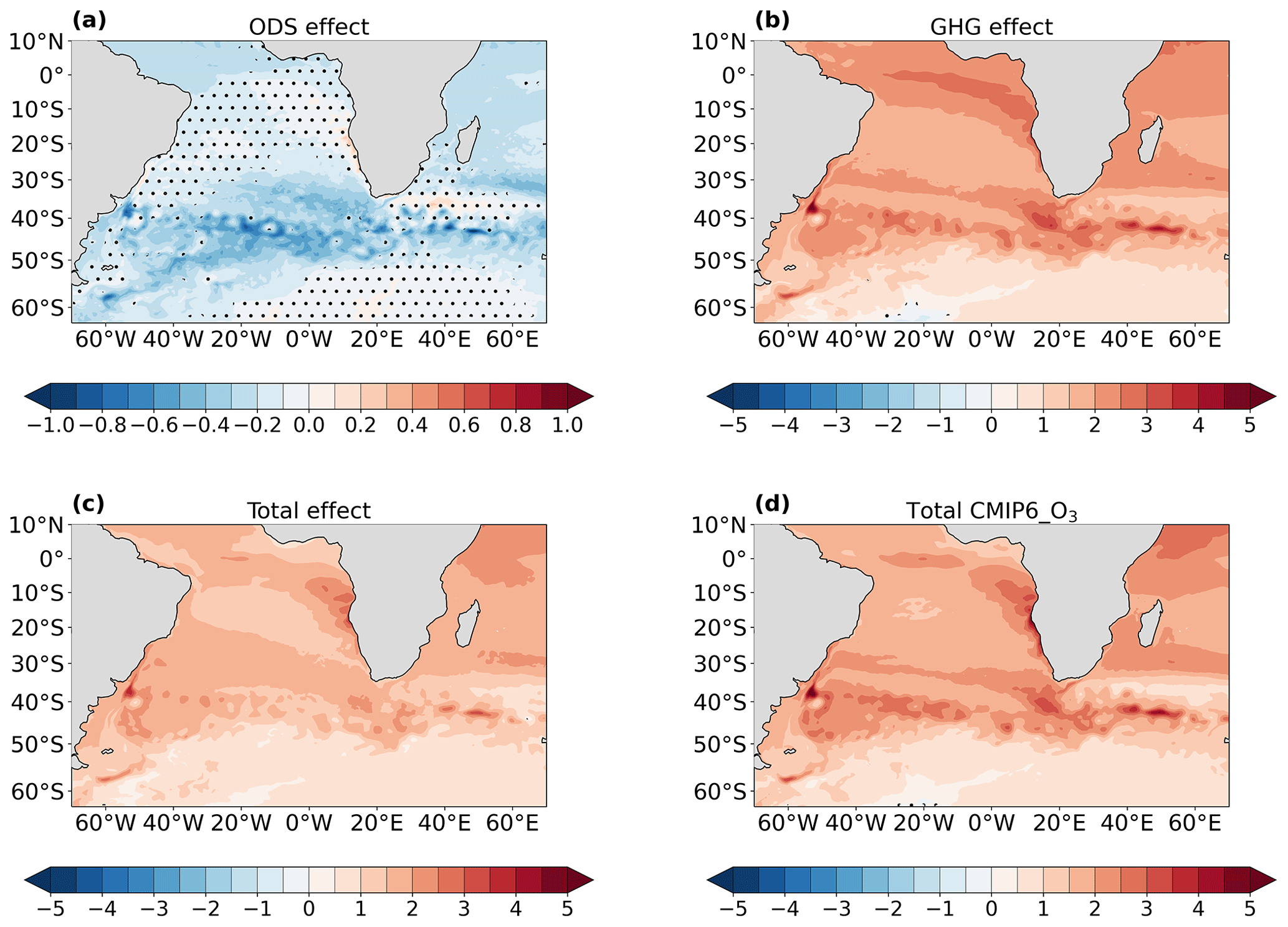
Figure 17 Changes in the SST (^∘C) for the region covered by the high-resolution nest (63^∘ S–10^∘ N and 70^∘ W–70^∘ E): effect of ozone recovery (a), effect of GHGs (b), total effect in INTERACT_O₃ (c), and total effect in CMIP6_O₃ (d). The stippling masks regions where the changes are not significant at the 95 % confidence interval based on a two-tailed t test.

The band of cooling (warming) at 45^∘ S due to ozone recovery (GHGs) extends down to about 1500 m (Fig. 18a and b). Observations and model simulations for the last decades exhibit a similar pattern of warming extending well below the surface (Armour et al., 2016; Li et al., 2016), attributed in part to ozone depletion (Bitz and Polvani, 2012; A. Solomon et al., 2015; Ferreira et al., 2015; Seviour et al., 2016; Li et al., 2021). Ozone recovery reverses this warming, but GHGs intensify it, such that the total effect continues to be an increase in the ocean temperature in this latitude band (Fig. 18c and d). As with the SST change, the warming is stronger in CMIP6_O₃ than in INTERACT_O₃. At this stage, we cannot fully isolate the reason for the warming around 45^∘ S. One one hand, the trade winds (arrows in Fig. S8) are affected by ozone recovery and GHGs. In combination with the changes in the westerlies, this leads to an intensification (weakening) and southward (northward) shift in the subtropical gyre due to GHGs (ozone recovery) (Fig. S9). On the other hand, the warming can also be explained by changes in Ekman transport and pumping associated with the wind changes (Fig. S8). The strengthening in both the westerlies and trades driven by GHGs leads to a stronger Ekman convergence, intensifying the downwelling between 40 and 50^∘ S. Ozone depletion is causing the opposite effects.

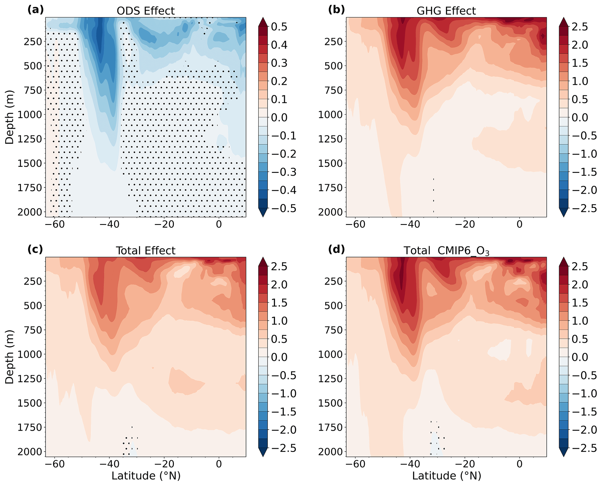
Figure 18 Latitude–depth profile of oceanic potential temperature changes (^∘C) zonally averaged over the high-resolution nest (70^∘ W–70^∘ E): effect of ozone recovery (a), effect of GHGs (b), total effect in INTERACT_O₃ (c), and total effect in CMIP6_O₃ (d). The stippling masks regions where the changes are not significant at the 95 % confidence interval based on a two-tailed t test.

5 Summary and discussion

The unique ocean–atmosphere coupled climate model FOCI with interactive ozone chemistry and a high-resolution ocean nest was used in this study to separate the effects of ozone recovery and increasing GHGs on the atmospheric and oceanic circulation in the SH during the twenty-first century under the high-emission scenario SSP5-8.5. A special emphasis was placed on the spatial patterns that characterize these effects. In addition, the combined effects of the two forcings were compared between the configuration of FOCI with interactive ozone chemistry and the configuration in which the CMIP6 ozone field consistent with the SSP5-8.5 pathway was prescribed.

The springtime Antarctic total column ozone in FOCI returns to 1980s levels in 2048 as increasing GHGs following SSP5-8.5 accelerate the recovery of the ozone hole by about 2 decades. In the upper stratosphere, the increase in GHGs contributes about half of the total ozone recovery over the twenty-first century in FOCI. This is explained by the GHG-induced cooling, which slows down the reactions involved in destroying ozone, as shown by Haigh and Pyle (1982), Rosenfield et al. (2002), Jonsson et al. (2004), and Revell et al. (2012). At lower-stratospheric levels, GHGs cause an increase in ozone through transport changes associated with an enhanced BDC.

Ozone recovery during the twenty-first century reverses the effects of the past ozone depletion, in agreement with previous studies (e.g., McLandress et al., 2010), leading to a warming of the lower-stratospheric polar cap in austral spring and a weakening of the westerly winds in both the stratosphere and the troposphere. In contrast, increasing GHGs drive a cooling of the stratosphere throughout most of the year and westerly wind anomalies peaking at the top of the subtropical jet and extending vertically to the surface and to the top of the stratosphere.

By analyzing for the first time the spatial patterns of changes during austral spring, we showed that GHGs have an important dynamical impact on the SH stratosphere during austral spring that differs from their effect during the rest of the year. The increase in GHGs leads to changes in the characteristics of planetary waves propagating from the troposphere into the stratosphere, mainly of the PW1, which experiences an eastward phase shift. As a result, despite their symmetric forcing, GHGs induce temperature and zonal wind anomalies of opposite sign over the Pacific and Indo-Atlantic sectors of the Southern Ocean, which are of similar magnitude to the ozone-induced anomalies. Therefore, the ozone and GHG effects reinforce each other over the Pacific sector and counteract each other over the Indo-Atlantic sector. Due to the PW1 structure of the stratospheric temperature and zonal wind changes that results from the increase in GHGs, these changes are severely underestimated when zonal or areal mean fields are analyzed. FOCI simulates a statistically insignificant warming in the lower stratosphere during October, when the temperature change due to GHGs is averaged over the polar cap, while Karpechko et al. (2010) reported a significant warming of the Antarctic lower stratosphere in their ensemble forced solely by increasing GHGs. In contrast, Son et al. (2008, 2009) found a weak cooling of the Antarctic lower stratosphere in the CMIP3 models that exclude ozone recovery, in agreement with McLandress et al. (2010), who also found that GHGs drive a weak polar cap lower-stratospheric cooling in their CCM. These contrasting results are likely explained by intermodel differences in simulating the changes in planetary wave activity due to GHGs, which result in temperature and zonal wind responses of different magnitudes in the different models.

Ozone recovery leads to a reduction in the flux of wave activity into the stratosphere during spring by weakening and causing an earlier breakdown of the polar vortex. As the height at which wave drag is being deposited as a result of wave breaking is decreased, the polar downwelling weakens during October in the upper stratosphere and during November and December throughout the entire stratosphere. The resulting dynamical cooling diminishes the warming that occurs due to the radiative effect of ozone in the lower stratosphere and causes an overall cooling of the upper stratosphere in these months. The analysis of the downward mass flux and of the mean residual stream function revealed that the entire residual circulation in the SH is weakened between October and December. Our results add to the body of evidence (Oman et al., 2009; McLandress et al., 2010; Lin and Fu, 2013; Oberländer et al., 2013; Polvani et al., 2018, 2019) that the consequence of ozone recovery during the twenty-first century will be to weaken the BDC and therefore partly offset the strengthening induced by the increase in GHGs. However, all of these studies reported that the contrasting effects on the BDC occur in austral summer. While we also find that GHGs strengthen and ozone recovery weakens the BDC in the SH during summer, the summer changes are small when compared to springtime changes, and, for the case of ozone recovery, they are dominated by changes during December. This result is in line with the presence of climatological easterlies in the middle and upper stratosphere throughout most of the summer that do not support Rossby wave propagation and therefore confine the changes in wave drag to the lower stratosphere, where the zero-wind line is located.

The increase in GHGs drives a strengthening of the SH residual circulation throughout most of the year, with the exception of November, when it leads to a weakening instead, reinforcing the weakening effect of ozone recovery during this month. Therefore, the combined effect of ozone recovery and increasing GHGs on the residual circulation is a weakening in November and December and a strengthening during the rest of the year. Our results highlight that the increasing GHGs play an important role in the dynamical stratospheric changes that take place in austral spring during the twenty-first century. The changes in the residual circulation and in the stratospheric polar night jet are mediated through changes in the propagation of planetary waves, in particular of the PW1. The exact mechanism through which the increase in GHGs alters the propagation of planetary waves is, however, not known. It is possible that the changes are triggered by the acceleration of the upper flank of the subtropical jet due to the radiative warming (cooling) of the upper troposphere (lower stratosphere) caused by GHGs. The non-linear character of the interactions between planetary waves and the zonal wind makes it difficult to understand how this acceleration then affects planetary wave propagation.

At the surface, our analysis of the twenty-first-century changes in the SH surface westerly winds supports previous findings (Shindell and Schmidt, 2004; Yin, 2005; Perlwitz et al., 2008; McLandress et al., 2011; Polvani et al., 2011a) that ozone recovery drives a weakening and equatorward shift in the westerlies accompanied by a negative change in the SAM during austral summer, while increasing GHGs drive a year-round strengthening and poleward shift accompanied by a positive change in the SAM. Under the high-emission scenario SSP5-8.5, FOCI projects that the GHG effect overwhelms the effect due to ozone recovery both during austral summer and in the annual mean, but the surface changes are weaker when both forcings are considered than those driven by GHGs alone. We note that the total change in the surface westerlies will depend on how much GHGs will increase in the future. Westerly wind changes in studies that also investigated low- to moderate-emission scenarios range from an equatorward shift to no significant changes (Eyring et al., 2013; Barnes et al., 2014; Gerber and Son, 2014; Iglesias-Suarez et al., 2016; Bracegirdle et al., 2020).

The Agulhas leakage is increasing during the twenty-first century. This increase is driven by the wind stress changes associated with the increasing GHGs and is partly offset by the effect of ozone recovery. Our composite analysis revealed that a stronger Agulhas leakage is associated with increased temperature and salinity in the southeastern South Atlantic. Our results are consistent with those of Biastoch et al. (2015) and Cheng et al. (2018), who related an increased Agulhas leakage to higher SSTs extending from the Cape Basin into the South Atlantic. We additionally showed that this relationship is also valid at depth, down to 1000 m. The link between increased Agulhas leakage and higher southeastern Atlantic temperatures simulated in FOCI in the upper 1000 m supports the findings of Lübbecke et al. (2015) that the positive Agulhas leakage trend in the second half of the twentieth century contributed to the warming of the eastern tropical Atlantic. However, the temperature anomalies are not detectible anymore in FOCI after 5 years. This could be partly explained by loss of heat to the atmosphere that damps the temperature anomalies, as reported by Weijer et al. (2002) and Biastoch and Böning (2013). The salinity anomalies, in contrast, are advected northwestward and can be detected in the central part of the South Atlantic at a lag of 5 years. This results in the development of positive density anomalies that are advected towards the North Atlantic and that can potentially be important for the stability of the AMOC as they have the ability to partially compensate the changes in density resulting from a freshening of the North Atlantic due to climate-change-induced ice sheet melting that causes less deepwater formation and hence a weaker AMOC. Unfortunately, in the current study, we cannot isolate the impact of the increase in Agulhas leakage on the AMOC from other effects of the increasing GHGs. Nevertheless, there is compelling evidence from previous studies that salinity anomalies related to an increased Agulhas leakage reach the subtropical North Atlantic within 2 to 4 decades (Biastoch and Böning, 2013; Weijer and van Sebille, 2014). In addition, 40 % of the Agulhas leakage was found to reach 24^∘ N within 2 decades (Rühs et al., 2013). Therefore, the twenty-first-century increase in Agulhas leakage has the potential to alter the thermohaline structure of the AMOC. In addition to the temperature and salinity changes arising from increased Agulhas leakage, we see a local effect driven by changes in the Ekman transport due to changing westerlies and trades. Ozone recovery reverses the warming caused by ozone loss north of the ACC and extending to intermediate depths (Ferreira et al., 2015; A. Solomon et al., 2015; Seviour et al., 2016; Li et al., 2021). In contrast, GHGs lead to warming in the same regions. The pattern of cooling due to ozone recovery closely matches the pattern of warming due to GHGs because they are both modulated by the respective changes in the surface wind stress, which have opposing signs and thus result in opposing circulation changes. The GHG effect is dominant, and when both drivers are considered together, the entire South Atlantic is warming.

The transport of the ACC in the Drake Passage and south of Africa is decreased by ozone recovery and increased by climate change, in agreement with the findings of Sigmond et al. (2011), but changes in transport are rather small, with a maximum of 6 %. The combined effect of ozone recovery and increasing GHGs equals the effect of GHGs alone. This result is consistent with the fact that the ACC is in an eddy-saturated state (e.g., Farneti et al., 2010; Morrison and Hogg, 2013) as the effects of an increase in eddy activity and of an increase in northward Ekman transport offset each other, rendering the ACC only weakly sensitive to changes in wind stress. Typically, coupled climate models such as those used for the different phases of CMIP have too low a resolution to simulate mesoscale eddies and rely on eddy parametrization schemes based on Gent and Mcwilliams (1990) to account for eddy effects (e.g., Downes and Hogg, 2013). CMIP5 models do not agree on the sign of the change in ACC transport during the twenty-first century under RCP8.5, with about half of the models simulating an increase and the other half simulating a decrease in transport (Downes and Hogg, 2013). Additionally, there is no statistically significant relationship between the change in the strength of the zonal wind stress and the change in ACC transport among the CMIP5 models (Meijers et al., 2012; Downes and Hogg, 2013). The ACC transport changes in the Drake Passage of about 6 % and 11 % in FOCI with interactive ozone and with prescribed CMIP6 ozone, respectively, fall within the range of changes of about ±15 % simulated by CMIP5 models under RCP8.5 (Downes and Hogg, 2013). Unlike the CMIP5 models, however, FOCI has a higher oceanic resolution, $\mathrm{1}/\mathrm{2}$^∘ globally and $\mathrm{1}/\mathrm{10}$^∘ within the high-resolution nest, INALT10X. The mesoscale eddies are resolved in the Atlantic sector and in part of the Indian sector of the Southern Ocean, and because of the two-way nesting technique used in FOCI, the information about the presence of the eddies is transmitted to the global ocean model. Therefore, we can assume that this configuration of FOCI captures the eddy saturation effect better than the CMIP-class models. Bishop et al. (2016) performed a perturbation experiment with another coupled climate model that uses a $\mathrm{1}/\mathrm{10}$^∘ oceanic resolution in which they increased the zonal wind stress over the Southern Ocean by 50 % and found only a 6 % strengthening in the ACC transport through the Drake Passage in response. In our simulations, a 6 % and an 11 % ACC transport increase is obtained for the wind stress increases of 10 % and 17 % in INTERACT_O₃ and CMIP6_O₃, respectively, implying that the sensitivity of the ACC transport to wind stress changes is stronger in our model. Although our results are not directly comparable with those of Bishop et al. (2016) because their simulation does not include changes in buoyancy due to, for example, climate change, this suggests that the degree of eddy saturation is further increased if the oceanic resolution is eddy-resolving over the entire Southern Ocean.

The comparison of the combined ozone and GHG effect between the ensemble with interactive ozone chemistry, INTERACT_O₃, and the ensemble in which the CMIP6 ozone field is prescribed, CMIP6_O₃, revealed that the ozone effect is weaker, and the GHG effect is more dominant in the latter ensemble, in agreement with the weaker increase in the ozone field in CMIP6. Significant differences were found in all of the examined fields. In the stratosphere, differences in both the magnitude and the spatial pattern of the total response occur. The magnitude of the difference at the surface and in the oceanic circulation is comparable to or greater than the ozone effect itself. This hints at the fact that other factors likely contribute to these differences, in addition to the difference in the ozone fields. Such possible factors are the interpolation of the prescribed monthly mean ozone field in time, which causes an underestimation of the spring ozone changes (Sassi et al., 2005; Neely et al., 2014); the feedbacks between the ozone field, radiation, and dynamics that cannot occur if the ozone field is prescribed and are therefore not properly captured (Haase et al., 2020); and the inconsistencies between the prescribed ozone field and the dynamics in the model (Ivanciu et al., 2021). In addition, the combined effect when the ozone field is prescribed is in some cases larger than the GHG effect simulated alone in the ensemble in which the ozone field is calculated interactively. This suggests that the GHG effect is affected by the response of the ozone field and is greater when the ozone is prescribed. The studies by Morgenstern et al. (2014) and Chiodo and Polvani (2016) showed that there are important dynamical changes resulting from the response of the ozone field to GHGs and that these changes offset part of the direct influence of GHGs on the SH dynamics. Although the prescribed CMIP6 ozone field is consistent with the increase in GHGs under SSP5-8.5, it cannot react to the changes in GHG concentrations during the simulations to which it is prescribed and may therefore be less sensitive to the GHG changes than in the ensemble in which it evolves interactively. This, in turn, could result in a lower degree of compensation between the direct GHG effect on the dynamics and the GHG effect mediated by the ozone field. While including interactive ozone chemistry is the only way to ensure that all ozone-related processes are simulated and that the ozone field is spatially and temporally consistent with the simulated dynamics, we showed that even larger uncertainties in future projections are related to estimates of ozone recovery itself. The CMIP6 ozone field has been produced by two CCMs, yet the Antarctic ozone returns to 1980s values in 2089, much later than in FOCI (2048) or in the CCMI ensemble average (2060; Dhomse et al., 2018). This shows how large the spread in ozone recovery rates is among CCMs. As a result, the magnitude of the effects of ozone recovery also exhibits a large spread, as demonstrated here using the same model with two different ozone fields.

The differences in the circulation response to ozone recovery and increasing GHGs between INTERACT_O₃ and CMIP6_O₃ show that the choice of the ozone field can affect the prediction of changes not only in the atmospheric but also in the oceanic circulation. This adds to the evidence provided by Ferreira et al. (2015), Li et al. (2016), and Seviour et al. (2016) that the ozone field affects the SH oceanic circulation. Furthermore, it suggests that the ozone field may introduce a source of uncertainty in the predictions for the twenty-first century.

While in the stratosphere the effects of ozone recovery and increasing GHGs reinforce each other in some regions and counteract each other in other regions, the GHG effect clearly dominates the changes at the surface and in the oceanic circulation under the high-emission scenario used here. However, these changes are considerably weaker in the presence of ozone recovery than in its absence, highlighting the importance of the Montreal Protocol in mitigating some of the impacts of climate change.