the Creative Commons Attribution 4.0 License.
the Creative Commons Attribution 4.0 License.
 | 15 Feb 2022
How well is Rossby wave activity represented in the PRIMAVERA coupled simulations?
Paolo Ghinassi
Federico Fabiano
Susanna Corti
This work aims to assess the performance of state-of-the-art global climate models in representing the upper-tropospheric Rossby wave pattern in the Northern Hemisphere and over the European–Atlantic sector. A diagnostic based on finite-amplitude local wave activity is used as an objective metric to quantify the amplitude of Rossby waves in terms of Rossby wave activity. This diagnostic framework is applied to a set of coupled historical climate simulations at different horizontal resolutions, performed in the framework of the PRIMAVERA project and compared with observations (ERA5 reanalysis). At first, the spatio-temporal characteristics of Rossby wave activity in the Northern Hemisphere are examined in the multimodel mean of the whole PRIMAVERA set. When examining the spatial distribution of transient wave activity, only a minimal improvement is found in the high-resolution ensemble. On the other hand, when examining the temporal variability of wave activity, a higher resolution is beneficial in all models apart from one. In addition, when examining the Rossby wave activity time series, no evident trends are found in the historical simulations (at both standard and high resolutions) and in the observations. Finally, the spatial distribution of Rossby wave activity is investigated in more detail focusing on the European–Atlantic sector, examining the wave activity pattern associated with weather regimes for each model. Results show a marked inter-model variability in representing the correct spatial distribution of Rossby wave activity associated with each regime pattern, and an increased horizontal resolution improves the models' performance only for some of the models and for some of the regimes. A positive impact of an increased horizontal resolution is found only for the models in which both the atmospheric and oceanic resolution is changed, whereas in the models in which only the atmospheric resolution is increased, a worsening model performance is detected.
- Article
(30137 KB) - Full-text XML
-
Supplement
(1984 KB) - BibTeX
- EndNote


The European continent is located at the downstream end of the North Atlantic storm track. Over this region, the variability of the large-scale circulation is characterized by the coexistence of low frequency planetary Rossby waves and higher-frequency transient eddies (Blackmon, 1976), the latter known as Rossby wave packets (RWPs; Pedlosky, 1972; see Wirth et al., 2018 for a recent review). Planetary Rossby waves have a zonal wavenumber between 1 and 3, and their phase speed is slower compared to RWPs. Planetary Rossby waves are forced by the orography (mountain ranges, land–sea contrast) and can be observed in the time-averaged circulation, manifesting as large meanders in the jet stream with a quasi-stationary phase (Edmon Jr et al., 1980; Hoskins and Karoly, 1981). RWPs on the other hand arise from the conversion of the available potential energy stored in the meridional temperature gradient found in the midlatitudes into kinetic energy through baroclinic instability (Simmons and Hoskins, 1979; Chang and Orlanski, 1993). RWPs have a zonal wavenumber greater than 4 (a typical value in the midlatitudes ranges between 4 and 8), and their life cycle typically occurs on a timescale of less than 10 d (Blackmon et al., 1984). Although some RWPs may manifest as circumglobal waves (especially RWPs excited by teleconnections; Wallace and Gutzler, 1981; Branstator, 2002), usually their amplitude appears localized in space (Lee and Held, 1993; Wirth et al., 2018). RWPs propagate along the sharp potential vorticity (PV; Hoskins et al., 1985) gradient associated with the jet stream in the upper troposphere. The concurring effect of all these waves with different characteristic spatial and temporal timescales is thus responsible for the complexity of the climate over the European–Atlantic (EAT) sector.
One way to analyse the climate variability characteristic of the midlatitudes is to partition the atmospheric circulation into weather regimes (WRs). In the last decade several authors analysed the ability of state-of-the-art climate models in representing the synoptic-scale climate variability in the midlatitudes using a weather regime (WR) approach (Dawson et al., 2012; Cattiaux et al., 2013; Strommen et al., 2019; Fabiano et al., 2020, 2021). WRs are recurrent and persistent circulation patterns with a timescale that ranges from a few to several days (up to 3–4 weeks; Straus et al., 2007). WRs can be computed using several techniques applied to different meteorological fields (e.g. wind, geopotential height, mean sea level pressure); for example, one of these approaches consists in applying a clustering algorithm to the geopotential height field on a pressure surface (Michelangeli et al., 1995; Fabiano et al., 2020), which is the general approach used in the present work, although with some small differences. WRs appear as a series of positive and negative anomalies of geopotential height which extend along the zonal and meridional directions. Therefore WRs can be viewed as different phases belonging to a Rossby wave train, containing both the contribution of planetary Rossby waves and transient RWPs.
WRs are of interest because they are associated with different types of weather at the surface, depending on the position of the circulation anomalies in the upper troposphere (Robertson and Ghil, 1999; Yiou and Nogaj, 2004; Cassou et al., 2010). This implies that the ability of climate models to correctly simulate the observed extratropical large-scale circulation in the mid-troposphere and upper troposphere is of fundamental importance for a reliable representation of regional climate. Furthermore, understanding how the atmospheric circulation changes in response to global warming is a prerequisite for regional climate predictions (Corti et al., 1999; Matsueda and Palmer, 2018; Fabiano et al., 2021). Recently, it has been debated how climate change can have an impact on the extratropical circulation in terms of changes in the jet stream position and intensity or in terms of amplitude or phase speed of Rossby waves. In particular, three different phenomena which may induce changes in the dynamics of the extratropical circulation in the Northern Hemisphere have been identified: the Arctic amplification (Serreze et al., 2009; Screen and Simmonds, 2010); the upper-tropospheric warming in the tropics, related to an increased deep convection (Li et al., 2019); and the cooling of the polar stratosphere, driven by changes in the concentration of ozone and greenhouse gases (Randel and Wu, 1999; Ivy et al., 2016).
Francis and Vavrus (2012) hypothesized that the recently observed reduction in the thickness difference between the North Pole and the midlatitudes related to the Arctic amplification could slowdown the jet stream and thus favour large-amplitude quasi-stationary Rossby waves, associated with more persistent weather at the surface. The authors found evidence of an increasing trend in the amplitude of Rossby waves in reanalysis data and a slowdown of their phase speed, estimating the wave amplitude using a geometric approach based on the displacement of a set of geopotential height contours (Francis and Vavrus, 2012, 2015). Subsequently, however, the hypothesis and results of Francis and Vavrus were questioned by other authors. The work of Barnes (2013) and Screen and Simmonds (2013), for example, demonstrated that the results of Francis and Vavrus depended on the metric used to quantify the wave amplitude, and no evidence of a wavier jet stream was found using other diagnostic methods. Barnes and Screen (2015) pointed out that the Arctic amplification is one of the processes which may influence the jet stream variability (and thus the variability related with RWPs and WR) and that the opposite situation found in the upper troposphere (i.e. a strengthening of the meridional temperature gradient due to the warming of the upper troposphere in the tropics and polar stratospheric cooling) can, on the other hand, intensify the jet stream. These contrasting results motivate us to use a robust diagnostic based on finite-amplitude local wave activity (LWA), which is able to objectively identify Rossby waves, as we will discuss in the following paragraph. The use of LWA allows us to perform a quantitative analysis of the spatial distribution and temporal evolution of Rossby waves during the last few decades in the observations and check whether these features are reproduced correctly in climate models or not.
Nakamura and collaborators proposed a novel theory of LWA which is certainly of interest for our problem (Nakamura and Zhu, 2010; Nakamura and Solomon, 2010; Huang and Nakamura, 2016). LWA in fact is defined in terms of meridional displacement of PV on a given quasi-horizontal surface (e.g. constant pressure or entropy) at each longitude; therefore it is certainly suitable to quantify the instantaneous local waviness of the atmospheric flow. LWA is able to identify Rossby waves of different wavelengths and to quantify their amplitude even when it becomes large or even finite (for example during wavebreaking or the formation of PV cutoffs). An advantage of LWA (which follows from the material conservation of PV) is that it is a conserved quantity in a frictionless and adiabatic flow; therefore it possesses an exact conservation relation (Nakamura and Solomon, 2010; Huang and Nakamura, 2016). Meanwhile, Chen et al. (2015), following the work of Nakamura and coauthors, formulated a LWA version replacing PV with geopotential height. This variant of LWA, despite being simpler to compute from data, does not satisfy an exact conservation relation as in the formulation of Nakamura and coauthors. Such geopotential-height-based LWA has been used by Chen et al. (2015) and Blackport and Screen (2020) to examine waviness trends in the midlatitudes, confirming no evidence of a wavier jet stream associated with an increased wave activity in recent years.
Ghinassi et al. (2018) extended the local wave activity (LWA) of Huang and Nakamura (2016) (which was originally developed in the quasi-geostrophic (QG) framework) to the primitive equations in isentropic coordinates, defining it in terms of meridional displacement of Ertel PV on a given isentropic surface. The use of isentropic coordinates surely adds some complexity to the analysis of RWPs; however the isentropic formulation was found to be more suitable when used in the context of predictability of RWPs (Ghinassi et al., 2018; Baumgart et al., 2019) with respect to the quasi-geostrophic one, since the former better identifies RWPs propagating along the sharp PV gradient at the tropopause, while the latter cannot be used in the subtropics (where the QG approximation is not satisfied), where Rossby waves may originate or migrate.
The aim of this work is to assess how well the large-scale circulation over Europe and the North Atlantic is represented in state-of-the-art high-resolution global climate models, using observations (reanalysis) as reference. We will analyse data from the PRIMAVERA project, whose goal is to investigate the impact of the horizontal resolution in representing the climate variability and related dynamical processes in climate models. Recently, Fabiano et al. (2020) investigated how the typical WRs observed over Europe are represented in the historical coupled PRIMAVERA simulations. The authors used metrics defined in the physical space (such as mean regime patterns, jet latitude distributions or blocking index) and in the regime phase space (such as the mean WR patterns, WR significance and variance ratios) to assess the models' performance. The present analysis extends the work of Fabiano et al. (2020), focusing on the variability of the upper-tropospheric large-scale flow in terms of Rossby waves associated with WRs. To achieve this, we will combine the WR diagnostic of Fabiano et al. (2020) with the LWA in isentropic coordinates of Ghinassi et al. (2018), which in the present work will be used as an objective metric for waviness.
The paper is organized as follows: in Sect. 2 we introduce and briefly describe the theory of LWA and WR and the methodology to compute them from meteorological data. In Sect. 3 we analyse and describe the spatio-temporal characteristics of the wintertime Rossby wave activity in the Northern Hemisphere starting from reanalysis data and in the historical coupled PRIMAVERA simulations. Then, in Sect. 4 the LWA diagnostic is applied in combination with WRs, examining the distribution of Rossby wave activity associated with each regime pattern in the PRIMAVERA simulations, using the observations as reference. Finally, Sect. 5 is dedicated to the discussion of our results and the conclusions.
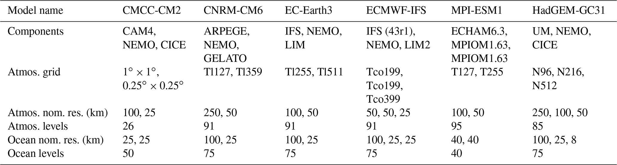
Table 1Models used in the analysis, listed with their components (atmosphere–ocean–ice models), the atmospheric grid used for the two versions (low- and high-res), the nominal resolution and the number of levels used for the atmosphere and ocean components. Note that for HadGEM-GC31 (LL, MM, HH) and ECMWF-IFS (LR, MR, HR) we also considered an intermediate-resolution run.
2.1 Dataset
We compare the following coupled climate models participating in PRIMAVERA: CMCC-CM2 (Cherchi et al., 2019), CNRM-CM6 (Voldoire et al., 2019), EC-Earth3 (Haarsma et al., 2020), ECMWF- IFS (Roberts et al., 2018), HadGEM3-GC31 (Williams et al., 2018) and MPI-ESM1-2 (Gutjahr et al., 2019). The simulations are performed with various nominal resolutions ranging from 250 to 25 km. For each model, we consider a standard-resolution (low-res, LR) run and one at higher resolution (high-res, HR). For ECMWF and HadGEM we also consider an intermediate-resolution run (MR) for both the atmosphere and the ocean. Additional information about model characteristics and their resolutions are available in Table 1. It is important to remark that in all PRIMAVERA simulations the horizontal resolution is changed with no additional tuning or adjustment of the models (HighResMIP protocol; Haarsma et al., 2020). Note that there is a great heterogeneity amongst the model resolutions; for example the LR runs for CMCC and HadGEM have a resolution of 250 km for the atmosphere, whereas the LR in ECMWF is only 50 km. Furthermore, most models increased the resolution of both the atmosphere and the ocean components, with the exception of CMCC-CM2 and MPI-ESM1, in which only the atmospheric resolution is increased. Several ensembles are produced for all models; however since we want to examine and visualize all WR patterns for all models, we consider only one member per model (the first for simplicity).
In our analysis we consider the coupled historical simulations, covering the period 1979–2015, comparing them with the ERA5 reanalysis (Hersbach et al., 2020) as reference. Daily data for winter months (DJF) are used for both PRIMAVERA simulations and reanalysis. Data used are the three-dimensional horizontal wind components, temperature and geopotential height fields. All variables are retrieved on a regular latitude–longitude grid with a 2∘ resolution for PRIMAVERA models and reanalysis. Pressure levels are 850, 700, 500, 250 and 100 hPa, which are the ones available in the PRIMAVERA dataset for daily data.
2.2 LWA
In this section, at first the theory of LWA is briefly recapped. In the primitive equations in spherical coordinates, where a is the Earth radius, λ is longitude, ϕ is latitude, t is time and potential temperature θ is a vertical coordinate, LWA is defined as (Ghinassi et al., 2020)
In the above definition,
is Ertel PV (Ertel, 1942; Hoskins et al., 1985), with denoting the isentropic layer density and ζθ the vertical component of isentropic relative vorticity. Q(ϕ,t) represents a specific value of PV, which at any time is uniquely related to a given latitude ϕ through
where dM=σdS is the isentropic layer mass in differential form. Δϕ represents the meridional displacement of a PV contour Q(ϕ) from latitude ϕ and can be multivalued when a PV contour intersects a meridian multiple times. Equation (1) states that LWA is proportional to the meridional displacement of PV contours Q from their associated latitude. LWA is phase dependent and quantifies the vigour of Rossby waves in terms of their pseudo-momentum (angular momentum per unit of mass), and its physical units are m s−1. LWA satisfies two important properties, which will be useful for the interpretation of our results. These properties are the generalized Eliassen–Palm relation (Andrews and Mcintyre, 1976) and the nonacceleration theorem (Charney and Drazin, 1961). The first relation describes the global conservation of LWA under conservative dynamics (in absence of nonconservative processes). The second theorem states that
or that the sum of and for conservative dynamics is locally constant (where the bar denotes some zonal averaging). This implies that an increase (decrease) in Rossby wave activity is associated with a reduction (acceleration) of the zonal wind.
To compute LWA, we start from the horizontal wind (u,v) and temperature on pressure levels, and then we interpolate the variables onto a selected isentropic surface following the steps described in Sect. 2 of Ghinassi et al. (2018). In this work, in contrast with Ghinassi et al. (2018), no zonal filter is applied to LWA to remove its phase information, since in this analysis we consider time-averaged fields (where the phase averaging is uninfluential) or we want to retain the phase information of LWA when examining the WR patterns. Unfortunately, the vertical resolution due to the available pressure levels in the PRIMAVERA simulations is quite coarse in the proximity of the tropopause. This implies a weaker isentropic PV gradient at the tropopause and translates into an underestimation of the real LWA magnitude. However, since the goal of our analysis is a model intercomparison, this does not affect the interpretation of our results, provided that all variables from PRIMAVERA simulations and reanalysis are retrieved on the same vertical levels.
Furthermore, LWA is partitioned into the stationary and transient components to quantify the wave activity contribution (transient vs. stationary) associated with each WR. The stationary component of LWA is estimated according to Huang and Nakamura (2017), as the LWA computed from the time mean (DJF) PV field. The transient LWA component is computed as the difference between the instantaneous LWA (i.e. the LWA computed from the instantaneous PV field on each day) and the stationary component of LWA.
2.3 Weather regimes
To compute weather regimes, we use the Python package named “WRtool” (available at https://github.com/fedef17/WRtool), and we closely follow the methodology described in Fabiano et al. (2020). In this work, however, instead of using geopotential height to define WRs, we use the Montgomery stream function (, Eq. 3.8.3 in Andrews et al., 1987, where cp = 1004 J kg−1 is the specific heat of dry air at constant pressure and Φ is geopotential) on the 320 K isentropic surface, to have a consistent framework with LWA, which is defined in isentropic coordinates.
We now briefly explain the algorithm to compute WR. At first, daily M anomalies are calculated as deviations from the seasonal cycle obtained from the 1979–2015 time series, smoothed with a 20 d running mean. Then the first four empirical orthogonal functions (EOFs) are calculated for M anomalies on the European–Atlantic Sector (EAT, defined as the box between 30 and 88∘ N and 80∘ W and 40∘ E) for reanalysis data. The first four EOFs for ERA5 explain 54 % of the total variance of M at 320 K.
To allow the comparison between different models and the observations, we choose to work with the same reference reduced phase space for all simulations, defined by the four leading EOFs obtained from ERA5 reanalysis. All M anomalies are projected onto this reference space, obtaining time series of principal components (PCs) for reanalysis and PRIMAVERA simulation data (we will refer to the model anomalies projected onto the reanalysis reference EOFs space as pseudo-PCs). Since the climatological mean field of M of each model is removed before this step, any mean state bias of the models does not affect the projection. As discussed in Fabiano et al. (2020), the choice of adopting the reference phase space for all models has some impact on some regime metrics and on the regime assignment (if the individual model's space differs substantially), but at the same time this guarantees a proper comparison of the regime patterns between the different models.
A K-means clustering algorithm is then applied to the reanalysis PCs and model pseudo-PCs, setting the number of clusters to four, which is commonly used in the literature (Michelangeli et al., 1995; Yiou and Nogaj, 2004; Cassou, 2008). Finally, WRs are attributed to the minimization of the distance in the reference phase space to the cluster centroid for all PCs and pseudo-PCs time series. The composites of the M anomalies of all the points belonging to the corresponding cluster, which are the mean WR patterns, are computed for both PRIMAVERA models and ERA5 data. The same is done for LWA, to obtain the spatial Rossby wave activity distribution corresponding to each regime.
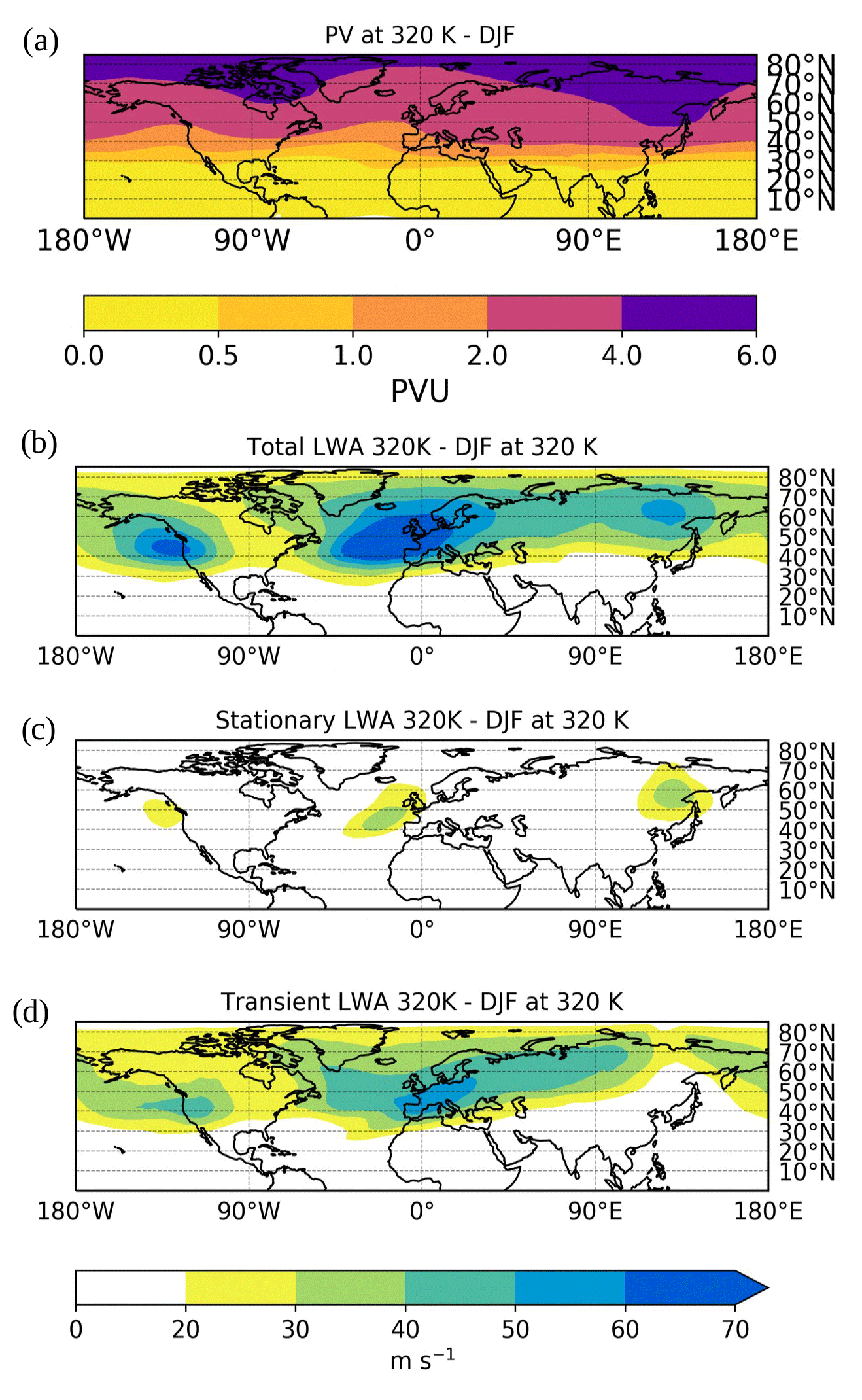
Figure 1Panel (a) shows time mean Ertel PV for DJF on the 320 K isentropic surface (in potential vorticity units (PVU), 1 PVU ≡ 10−6 kg K m2 s−1); panel (b) shows total (i.e. stationary and transient) LWA (colour, units m s−1) on the 320 K isentrope for DJF. Panel (c) is the same as (b) but for stationary LWA. Panel (d) is the same as (b) but for transient LWA.

Figure 2Multimodel mean of total LWA at 320 K for PRIMAVERA LR and HR (panels a and b) and for transient LWA (panels c and d). Black contours are the multimodel mean bias with respect to ERA5 (contour intervals every 5 m s−1; negative values are dashed). Stippling denotes the grid points in which the LWA bias is significant (i.e the bias is larger than the standard error in ERA5).
The LWA diagnostic is at first applied to the observed (i.e. using reanalysis data) northern hemispheric wintertime time-averaged flow, to visualize how the circulation in the upper troposphere appears in terms of PV and LWA. Figure 1a shows Ertel PV on the 320 K isentropic level for DJF computed from ERA5 data. We selected the 320 K isentropic surface since it intersects the tropopause in the midlatitudes, which is a desirable property when diagnosing Rossby waves using LWA (Ghinassi et al., 2018; see also Appendix A). A planetary stationary wave with wavenumber 2, associated with the Pacific and North Atlantic storm tracks, is clearly evident. The meridional PV gradient appears stronger in the upstream part of the two storm tracks (over eastern Asia and the east coast of North America) and more relaxed downstream, as we proceed towards the exit region of both storm tracks (i.e. over the northeastern Pacific and over Europe). These downstream regions are characterized by a broad PV ridge associated with an anticyclonic circulation in the time mean. The meridional PV gradient here appears weaker due to the PV mixing induced by the eddies (Novak et al., 2015), and wavebreaking is also frequent over these regions (Martius et al., 2007; Strong and Magnusdottir, 2008), often manifesting with PV streamers and PV cutoffs (Wernli and Sprenger, 2007). The total LWA (Fig. 1b) clearly maximizes at the downstream end of the storm tracks. This is a well known property of LWA, which tends to emphasize the mature (large amplitude) stage of the eddies (Huang and Nakamura, 2016; Ghinassi et al., 2018). A band of LWA extends from Europe until Siberia across Eurasia, likely to be associated with decaying finite-amplitude eddies penetrating into the Eurasia continent until reaching Siberia. Here, a secondary maximum of LWA, associated with a PV trough over the upstream part of the pacific storm track, is found. We now partition LWA into its stationary and transient components as described at the end of Sect. 2.2. Stationary LWA (Fig. 1c) exhibits 3 distinct maxima: two at the beginning and at the end of the Pacific storm track and a third one over the North Atlantic reaching western Europe. These maxima of stationary LWA are associated with a couplet of PV troughs–ridges found in the upstream and downstream regions of both storm tracks. The LWA associated with the PV trough over the eastern part of North America does not appear in the map since its magnitude is too weak. Transient LWA (Fig. 1d) has a stronger magnitude compared to its stationary counterpart, and it is found over a much larger portion of the domain. This implies that in the time mean picture transient eddies give the largest contribution to the total LWA in both storm tracks. Two maxima of transient LWA are found: one over the west coast of North America, extending towards the Rocky Mountains, and another one over Europe. Transient LWA in the North Atlantic storm track is much more longitudinally extended compared to the Pacific one, suggesting that transient RWPs tend to travel longer distances over the Eurasian continent, whereas at the end of the Pacific storm track the Rockies act to suppress transient Rossby wave activity immediately downstream of the mountain range. These results are in good agreement with Huang and Nakamura (2016), although the authors used the quasi-geostrophic formulation of LWA and considered the vertically integrated LWA (while here we focus only on the upper troposphere).
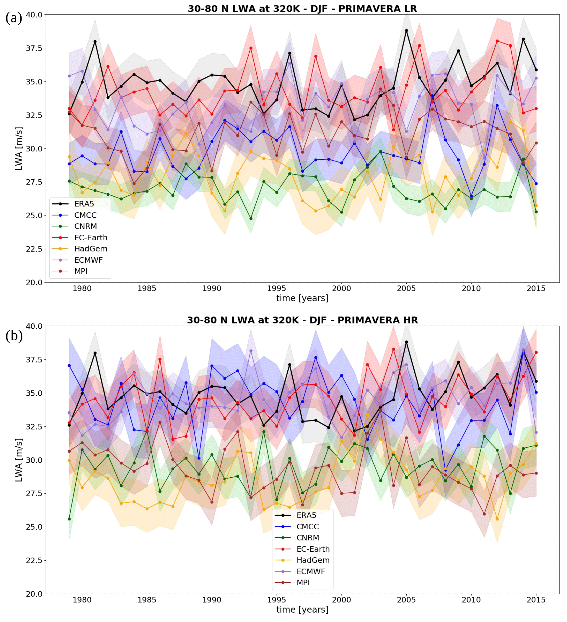
Figure 3Time series of transient LWA averaged over the NH. Each dot represents the time-averaged value for each winter season (DJF). The black line is ERA5, and PRIMAVERA models are in colour. Shading is the range between 2 standard deviations from the mean for each time series.

Figure 4Panel (a) box plot of the seasonal means of transient LWA averaged over NH. The dots are the mean values, the horizontal line in the boxes represents the median, the boxes are the first and third quartiles, and the bars are the 10th and 90th percentiles of the distribution. The left boxes are for each PRIMAVERA model (lighter colours are the LR runs, darker colours the HR). The first (black box) on the right refers to ERA5. The other two boxes represent average quantities among all the lowest-resolution (LR) and highest-resolution (HR) model versions and are calculated as the average of the percentiles and median over all models. Panel (b) shows the grouped box plot following the nominal atmospheric resolution of each model: each box represents the average percentiles and median over all models in that group. ERA5 is shown on the left for reference. In this case models with intermediate horizontal resolutions (ECMWF and HadGEM) are considered.
Now we move on to investigate how the Rossby wave activity is represented in PRIMAVERA. Figure 2 shows the multimodel mean of total and transient LWA in the Northern Hemisphere for the PRIMAVERA LR and HR simulations (colour) and its bias with respect to the observations (contours). The multimodel mean is obtained averaging the (time-averaged) LWA fields over all models, whereas the bias is computed as the LWA difference between the multimodel mean and ERA5 reanalysis. Generally, the main spatial features of the total LWA are represented correctly in both the PRIMAVERA LR and HR means. The total LWA maxima are found over the same regions of the observations; however their magnitude is weaker. The HR helps to reduce this bias, especially in the North Atlantic and over Europe, reducing the LWA difference with respect to ERA5 in the HR mean and strengthening the total LWA maximum over this sector (compare panel Fig. 2a with Fig. 2b). The total LWA over the Pacific is underestimated in both the LR and HR mean, and an increased resolution does not reduce this bias, as it even slightly increases it. When examining the plots of transient LWA (panels Fig. 2c and d), instead the picture is slightly different. As for the total LWA, both the LR and HR simulations are deficient in reproducing the transient LWA associated with the Pacific and North Atlantic storm tracks, but in this case an increased resolution provides only a small reduction in the transient LWA bias compared to reanalysis. In the HR mean the increased resolution helps to reduce the bias over the EAT sector. The transient LWA overestimation over Siberia is reduced, and transient LWA is slightly increased over Europe. Nevertheless the spatial distribution of transient LWA over the North Atlantic still appears too shifted inland to the east. Overall, the improvement in representing the total LWA observed in the HR mean seems to be mainly associated with a better representation of stationary LWA, especially over the EAT sector. The lack of a clear benefit of an increased resolution in the ability to correctly simulate transient LWA over the EAT sector motivates us to investigate this in more detail. In Sect. 4 we will examine the performance of PRIMAVERA models one by one, to reveal whether the weak signal observed in the HR mean is a common characteristic of all models or of only a subset of them (i.e. the weak signal observed in the mean is a result of cancellation). We will also include a WR analysis to investigate if there are circulation patterns which are particularly sensitive to an improvement or deterioration of the Rossby wave activity pattern depending on the horizontal resolution. Lastly, after analysing the spatial distribution of LWA, we investigate the temporal behaviour of LWA. To achieve this, time series of the averaged LWA,
(where 𝒟 is a certain domains and dS=a2cos ϕdϕdλ is the area element in spherical coordinates) are produced for the midlatitudes of the NH (between 30 and 80∘ N) for both PRIMAVERA models and the reanalysis.
Figure 3 shows the LWA time series for the wintertime-averaged LWA in ERA5 (black line in Fig. 3a and b) and PRIMAVERA (LR runs in Fig. 3a, HR in Fig. 3b). Regarding the magnitude of averaged LWA, it can be seen how in general PRIMAVERA LR models tend to underestimate LWA compared to reanalysis. An increased resolution appears to be beneficial, since comparing panel Fig. 3b with Fig. 3a, the HR simulations show a LWA magnitude which is closer to the observed one (particularly evident for the CMCC and CNRM models).
Figure 4a summarizes the model performances in reproducing the total LWA in the NH. For each model, the lighter colour corresponds to the LR run and the darker colour to the HR. At the right end of the plot, a measure of the observed variability (black box, named “ERA5”) is shown along with the average of the lowest- and highest-resolution versions of each model. It can be seen how the box plot confirms that an increased resolution is beneficial for almost all models (apart from the MPI model) to bring the LWA magnitude closer to observations. In order to explore the dependence of (spatially averaged) LWA with resolution, in Fig. 4b we classified the PRIMAVERA models according to their atmospheric horizontal resolution (see also Table 1) in four groups: lower resolution (250 km), standard resolution (100 km), higher resolution (50 km) and highest resolution (25 km) (as in Scaife et al., 2019). It can be seen how the magnitude of the northern hemispheric LWA converges towards the observations as the atmospheric resolution is increased. Two increments are observed in the magnitude of LWA: the first when the resolution is increased from 250 to 100 km and the second between 50 and 25 km.
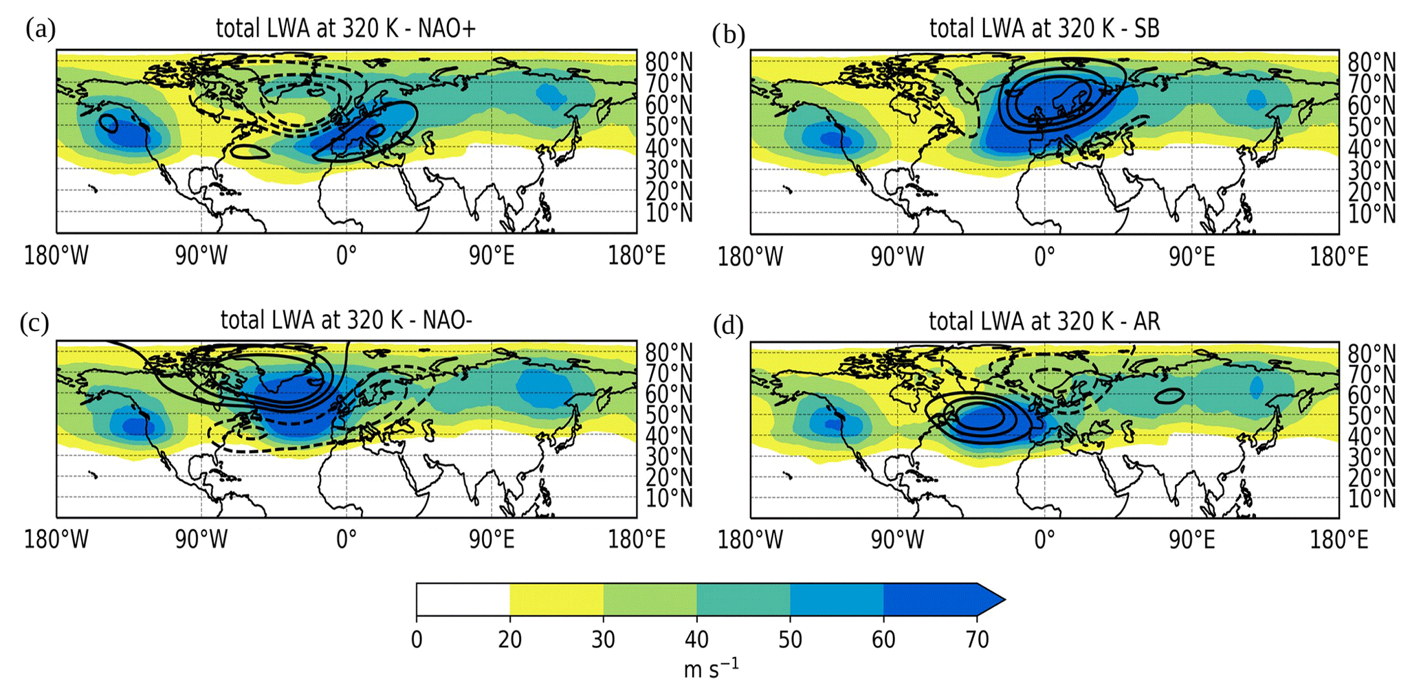
Figure 5Total (i.e. stationary and transient) LWA (colour, units m s−1) and Montgomery stream function anomalies (black contours at 500, 1000 and 1500 m2 s−2; dashed contours represent negative values; the zero contour is omitted) at 320 K associated with the four WRs over the EAT sector during winter in ERA5.
Furthermore, the temporal evolution of LWA in the Northern Hemisphere is investigated, including significant trends. A Mann–Kendall test has been performed on the time series, with p values of 0.38 for ERA5, between 0.16 and 0.90 for PRIMAVERA LR, and between 0.013 and 0.48 for PRIMAVERA HR. In two of the HR simulations, ECMWF and EC-Earth, a p value ≤ 0.05 is found, which could suggest a statistically significant positive trend; however, the magnitude of such a LWA trend is extremely weak (0.05 ). No significant trend emerges from the analysis of the LWA time series in reanalysis and PRIMAVERA models, with the oscillations likely to be related with the interannual variability of Rossby wave activity. As we discussed in the introduction, LWA is a particularly robust metric to quantify waviness since its temporal evolution can be clearly partitioned into conservative vs. nonconservative propagation (Eq. 15 in Ghinassi et al., 2020). A steady LWA in the time mean picture therefore suggests a zero net effect on LWA caused by nonconservative sources and sinks of LWA, since conservative dynamics can only rearrange the Rossby wave activity distribution. An increase or decrease in LWA with time, on the other hand, would imply an imbalance between sources and sinks of LWA during the examined period.
We now restrict our attention over the EAT sector and analyse the large-scale wintertime flow in terms of stream function anomalies and LWA associated with the four weather regimes. The four weather regime patterns computed from reanalysis data using the Montgomery stream function on the 320 K isentrope are almost identical to the ones obtained using geopotential height at 500 hPa (Cassou, 2008; Fabiano et al., 2020). These are the positive and negative phases of the North Atlantic Oscillation (NAO+ and NAO−, respectively), the Scandinavian blocking (SB) and the Atlantic Ridge (AR). The only difference found lies in the frequencies of WR, which, when computed using M, are 28.30 % for NAO+, 28.18 % for SB, 22.67 % for NAO− and 20.85 % for AR. Compared to Fabiano et al. (2020) we found a higher NAO− frequency than for the AR (although the frequencies of the two regimes are very close). This could be due to the fact that our analysis focuses on the upper troposphere (the 320 K isentropic surface is located roughly at 300 hPa in the midlatitudes during winter; see Fig. A1 in Appendix A) and the fact that we are using a different reanalysis dataset and consider a different period.
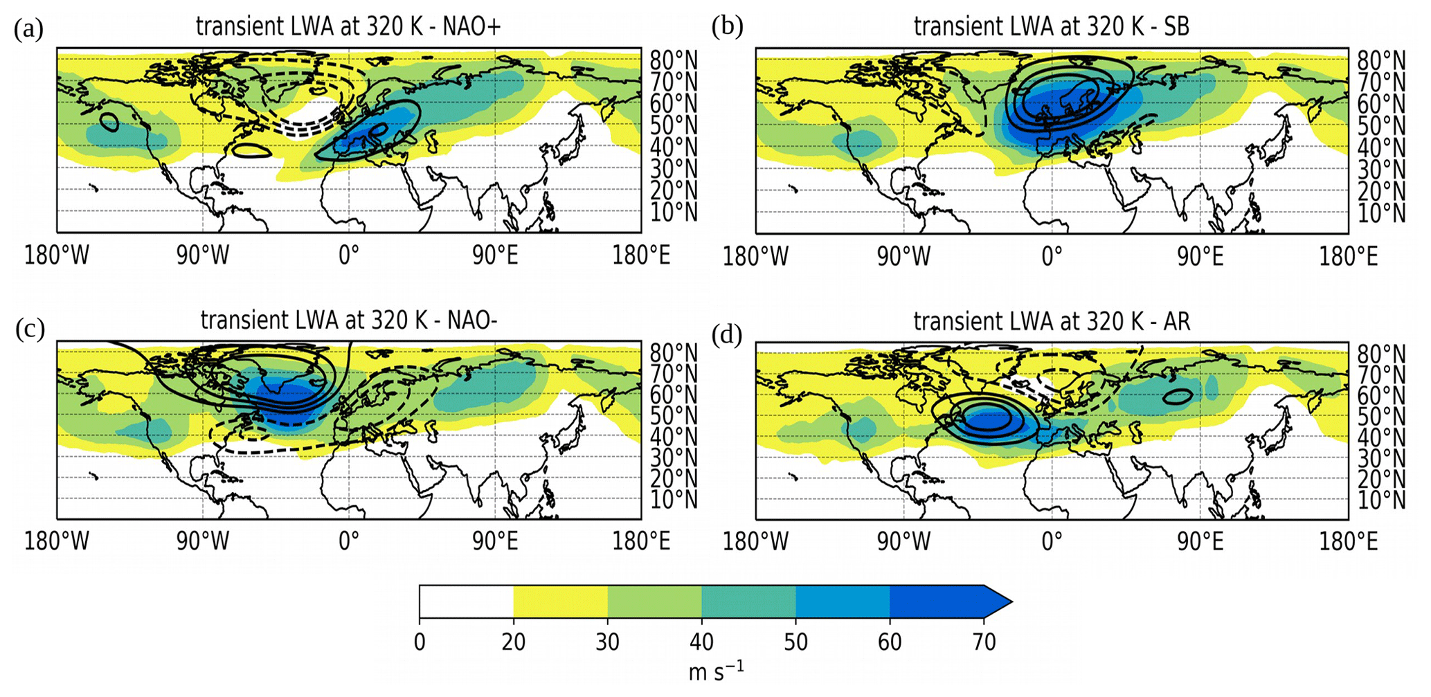
Figure 6Transient LWA (colour, units m s−1) and Montgomery stream function anomalies (black contours at 500, 1000 and 1500 m2 s−2; dashed contours represent negative values; the zero contour is omitted) at 320 K associated with the four WRs over the EAT sector during winter in ERA5.
Figures 5 and 6 show the M anomalies (contours) and the total and transient LWA (colour) associated with the four WRs. At a fist glance it can be seen how, again, total LWA maximizes over the anticyclonic phases of the regimes, while cyclonic anomalies tend to have a weaker LWA magnitude. This is particularly evident for the transient LWA component, which is very weak corresponding with the cyclonic M anomalies. Note that the stream function anomalies are very weak outside the EAT domain considered, whereas a strong signal is also found outside the EAT sector when examining LWA. In particular, a band of LWA extending over Eurasia and another maximum over the downstream region of the Pacific storm track are found in all four WR composites. If the position of the LWA band over central Eurasia does not seem to change significantly, the location of the secondary LWA maximum over the Pacific varies slightly in the four WRs. As can be seen comparing all panels of Fig. 5 with the corresponding ones of Fig. 6, such variability over the Pacific is mainly linked with the transient LWA component.
We now describe in more detail the large-scale circulation associated with each WR.
-
NAO+. In terms of stream function this regime is characterized by a broad cyclonic vortex in the North Atlantic and a narrow band of positive anomalies over southern and central Europe. LWA maximizes over this anticyclonic stream function anomaly. The cyclonic M anomaly in the North Atlantic appears mainly associated with the stationary LWA component (since it is visible in the total LWA map, Fig. 5a, but appears very weak in terms of transient LWA, Fig. 6a), whereas anticyclonic M anomalies are mainly associated with transient LWA (see Figs. 2 and 3). This band of anticyclonic LWA is likely to be associated with anticyclonic Rossby wave breaking over southern Europe and the Mediterranean. LWA in the North Atlantic is very weak (transient LWA is almost suppressed), consistent with a tilted jet stream deviating to the north with the characteristic SW–NE axis (remember that LWA and u are anti-correlated due to the nonacceleration theorem). Over the Pacific, a band of zonal transient LWA extends upstream of the Rockies.
-
SB. LWA maximizes over the wide anticyclonic stream function anomaly extending from the middle of the North Atlantic to the British Isles and Scandinavia. Both stationary and transient LWA contributes to the total LWA associated with SB. The former is mainly located over the western flank of the block, whereas the latter is found more in the centre and eastern flank of the structure. The high LWA values over the North Atlantic imply a very weak jet stream. A band of transient LWA is found downstream of the SB, linked with the band of negative M anomaly found over the Mediterranean. Over the Pacific transient LWA appears weaker compared to NAO+, with a maximum over the US portion of the Rocky Mountains.
-
NAO−. In terms of M and LWA it is similar to a SB pattern, but the whole structure is shifted to the west. A broad area of LWA is found over southern Greenland and in the middle of the North Atlantic. The wave activity pattern is characterized by an anticyclonic circulation on its poleward flank and cyclonic circulation on its equatorward flank. LWA is found poleward of the negative M anomaly in the North Atlantic, consistent with a zonal jet stream displaced at southern latitudes. LWA over the Pacific extends downstream of the Rockies towards Canada and Greenland, forming a “corridor” of LWA, which reaches the Atlantic basin.
-
AR. In terms of stream function the AR appears as a region of positive anomalies over the North Atlantic, south of 55∘ N. This large anticyclone extends in longitude from the east coast of North America to the Mediterranean across the Atlantic. Over this ridge a maximum of LWA is found, extending from the Atlantic and reaching the Mediterranean, consistent with a weaker jet over these regions. A large negative M anomaly is found to the NE of the ridge, between Greenland and Scandinavia. The LWA associated with this cyclonic vortex is mainly stationary (compare total and transient LWA plots for AR in Figs. 5d and 6d).
Now we proceed to examine how LWA associated with the four EAT WRs is represented in the PRIMAVERA models, focusing on the main differences observed when the horizontal resolution is increased. As anticipated in Sect. 3, in our comparison we focus only on transient LWA associated with RWPs, since the benefit of a higher resolution is less evident in the transient LWA distribution of the multimodel mean (compare Fig. 2c and d).

Figure 7Pattern correlation of transient LWA on the 320 K isentropic surface associated with the four WRs over the EAT sector during winter. Lighter colours are the LR simulations whereas darker colours are the HR ones.
Before starting our analysis, we verified that the differences in the height of the selected isentropic level are negligible between reanalysis and PRIMAVERA (see Appendix A). Then, we examined the spatial pattern correlation between the mean transient LWA pattern in each PRIMAVERA run against ERA5, which is shown in Fig. 7. It can be seen how the majority of the PRIMAVERA models represent the transient LWA pattern in a satisfactory way, with values of pattern correlation larger than 0.6 (apart from the CMCC model for the AR regime and NAO+ in the HR), with some of the models having a correlation larger than 0.8 (the best model in this sense is EC-Earth, which has a correlation coefficient larger than 0.8 for all four WRs). SB and NAO− are the regimes with the higher pattern correlation, whereas NAO+ and AR have slightly lower values on average. In some models and for some regimes, the HR simulations have a higher pattern correlation than the LR runs, suggesting that an increased resolution may improve the representation of the transient wave activity pattern associated with WRs. The improvement of the LWA pattern correlation with resolution however is not systematic in all models. In EC-Earth for example it is almost ineffective for all regimes. Then, there are some exceptions in which the HR run has a lower pattern correlation than the LR, for example in the MPI model (all regimes apart from AR), the CNRS model (NAO− and AR) and the CMCC model (all regimes apart NAO−). The CMCC HR run also fails almost completely to represent the transient LWA pattern associated with the AR.
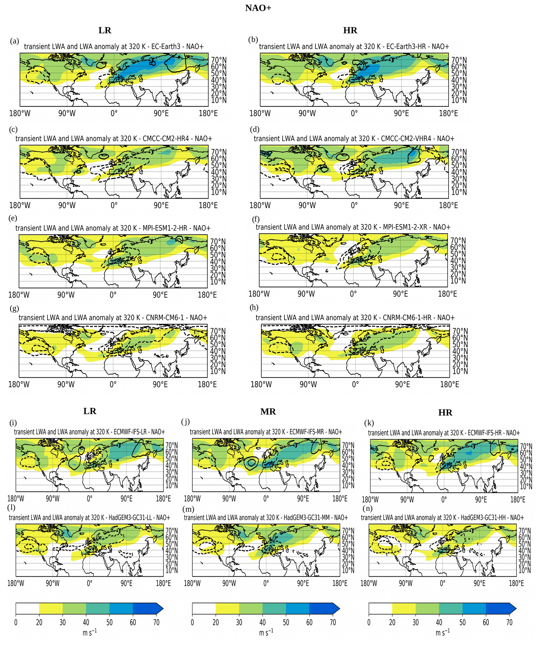
Figure 8Transient LWA (colour, units m s−1) and transient LWA anomalies with respect to ERA5 (black contours every 10 m s−1; dashed contours represent negative values) at 320 K associated with NAO+ for PRIMAVERA.

Figure 9As in Fig. 8 but for SB.
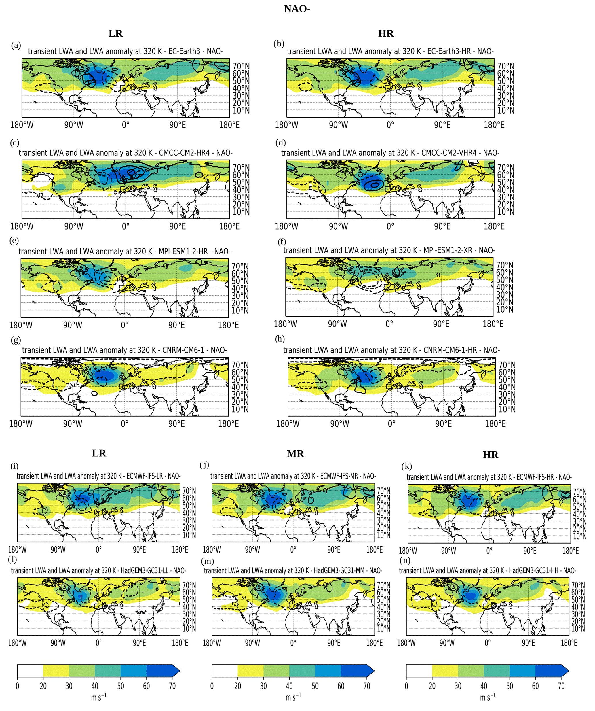
Figure 10As in Fig. 8 but for NAO−.
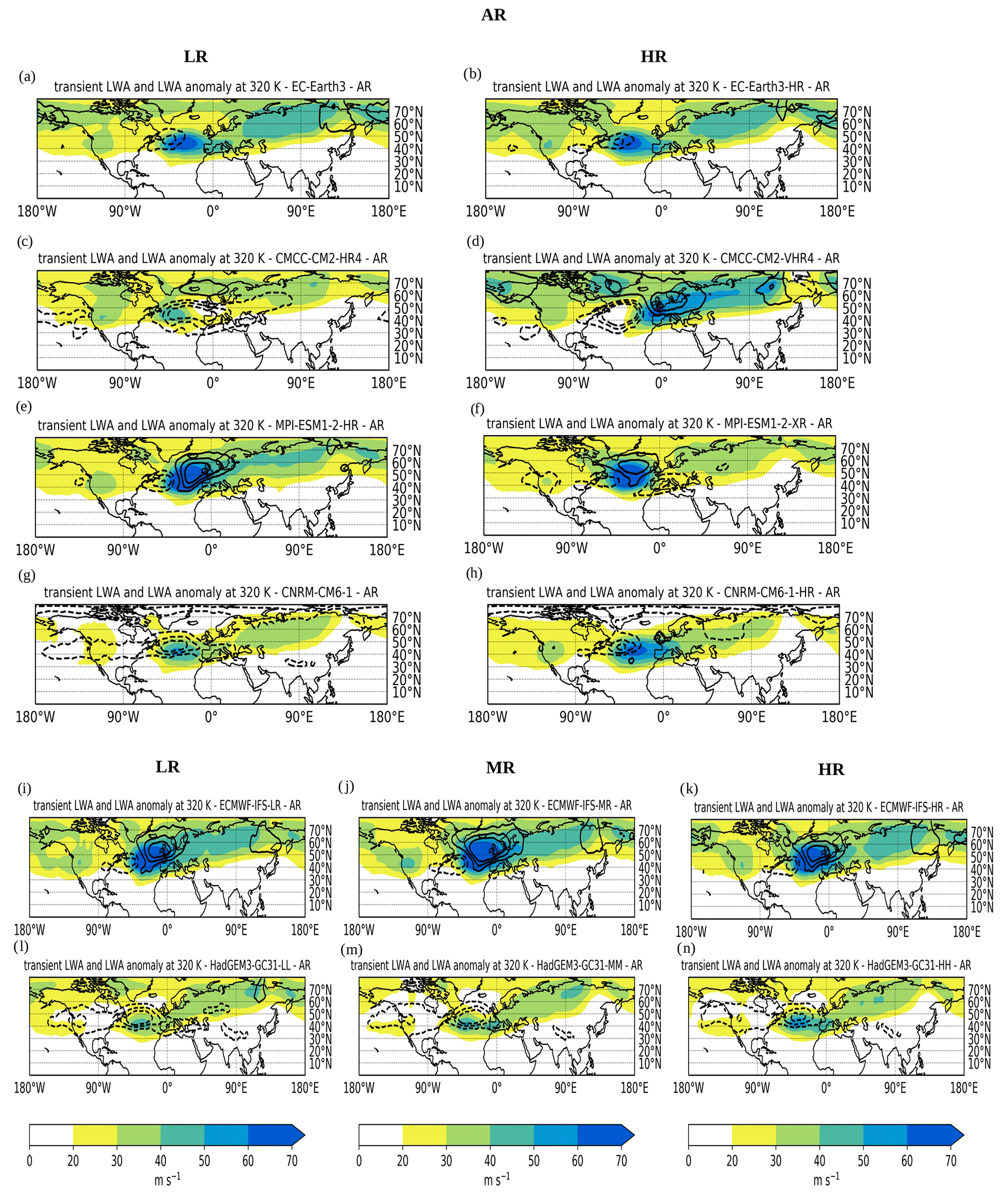
Figure 11As in Fig. 8 but for AR.
Now that we examined the LWA pattern correlation we move on the visualization of spatial maps of transient LWA for each regime and model. The pattern correlation in fact, despite being a concise metric to assess model performance, does not provide any information about the spatial distribution of LWA in the different models. Figures 8–11 show the transient LWA associated with NAO+, SB, NAO− and AR, respectively, for all PRIMAVERA simulations (LR and HR runs for all models; for ECMWF and HadGEM we show also the simulations at intermediate resolution) in colour, while black contours represent the models' bias with respect to ERA5. Due to the large number of maps to analyse, we will not discuss all of them in detail, but instead we will summarize the salient results for each regime in the following paragraph.
-
NAO+. EC-Earth is a good example of how an increased resolution is beneficial in improving the spatial LWA distribution. Despite there being almost no difference in the pattern correlation between the LR and HR over the EAT sector, transient LWA maps reveal how the tail of transient LWA which extends downstream over central and eastern Asia is reduced in the HR run (compare Fig. 8a and b). At the same time, the anticyclonic LWA over southeastern Europe appears weaker in both the LR and HR simulations compared to ERA5. In the CMCC model instead (Fig. 8c and d) the HR run seems to perform worse than the LR. In both resolutions transient LWA has a too-weak magnitude, but the HR run fails almost completely to reproduce the anticyclonic LWA over eastern Europe, which is also found further downstream over Eurasia. ECMWF (Fig. 8i–k) has a too-strong LWA on the equatorward flank of the jet in the North Atlantic and a too-weak LWA over Europe, presumably due to an overestimation of anticyclonic wave breaking during the NAO+ phase. An increased resolution here appears to reduce this bias. HadGEM (Fig. 8l–n) has an underestimation of LWA over the whole North Atlantic storm track, and an increased resolution clearly improves the model performance in simulating LWA over the Atlantic, but only slightly over Europe.
-
SB. EC-Earth is almost perfect in representing the magnitude and location of LWA associated with the block in both the LR and HR simulations (Fig. 9a and b, respectively). All other models (apart from CMCC) do a fair job in representing the pattern associated with blocking, but they underestimate the vigour of LWA on the western side of the block. In the ECMWF model (Fig. 9i–k), an increased resolution strengthens and broadens the LWA associated with blocking, reducing the bias. HadGEM correctly reproduces the location of the block but underestimates its magnitude in all three resolutions (Fig. 9l–n). The CMCC model, despite having a good LWA spatial correlation over the EAT sector, almost fails to represent the Rossby wave activity pattern in the NH in both the LR and HR simulations, and an increased resolution seems to even worsen the model performance (compare Fig. 9d with Fig. 9c).
-
NAO−. Almost all models succeed in reproducing the couplet of anticyclonic LWA over southern Greenland and the area of suppressed transient LWA immediately downstream over Europe. However, a common feature observed in the majority of the models (especially EC-Earth, ECMWF or MPI LR) is to underestimate LWA on the eastern or southeastern flank of the anticyclone. In the HR runs of ECMWF (Fig. 10k) and EC-Earth (Fig. 10b) this bias is reduced, while in MPI the HR performs worse, with the NAO− pattern which is almost completely wrong (Fig. 10f). The CMCC model is certainly the one in which the best improvement is observed upon increasing the horizontal resolution (compare Fig. 10c and d).
-
AR. This is the regime where the PRIMAVERA models exhibit the largest variability in representing the spatial LWA pattern. EC-Earth (Fig. 11a for LR and Fig. 11b for HR) and MPI (Fig. 11e for LR and Fig. 11f for HR) models seem to have the best performance in representing the LWA distribution linked with AR; however the former underestimates the LWA magnitude while the latter overestimates it. In both cases these biases are not corrected in the HR simulations. HadGEM (all resolutions, Fig. 11l–n) and CNRM (Fig. 11g and h) correctly reproduce the AR pattern in terms of stream function; however LWA appears too weak compared to reanalysis. ECMWF (Fig. 11i–k) on the other hand correctly captures the LWA pattern associated with the AR regime, but it substantially overestimates its intensity. Finally, note how the CMCC model HR (Fig. 11d) completely fails to represent the AR pattern, and an increased resolution leads to a poorer model performance (pattern correlation for the AR in the CMCC HR run is close to zero; see Fig. 4).
Finally, note how the LWA pattern over the downstream region of the Pacific storm track appears much weaker and smeared out compared to the reanalysis in all simulations, and no clear, spatially localized secondary maximum of LWA can be identified over this region, as it was for the PRIMAVERA multimodel mean.
In addition to the analysis of WR in terms of transient LWA, we repeated our approach but considering only the transient LWA anomaly (i.e. the transient LWA in each WR minus the climatology of transient LWA for DJF) to exclude the model biases in the mean state. The results are presented in the Supplement.
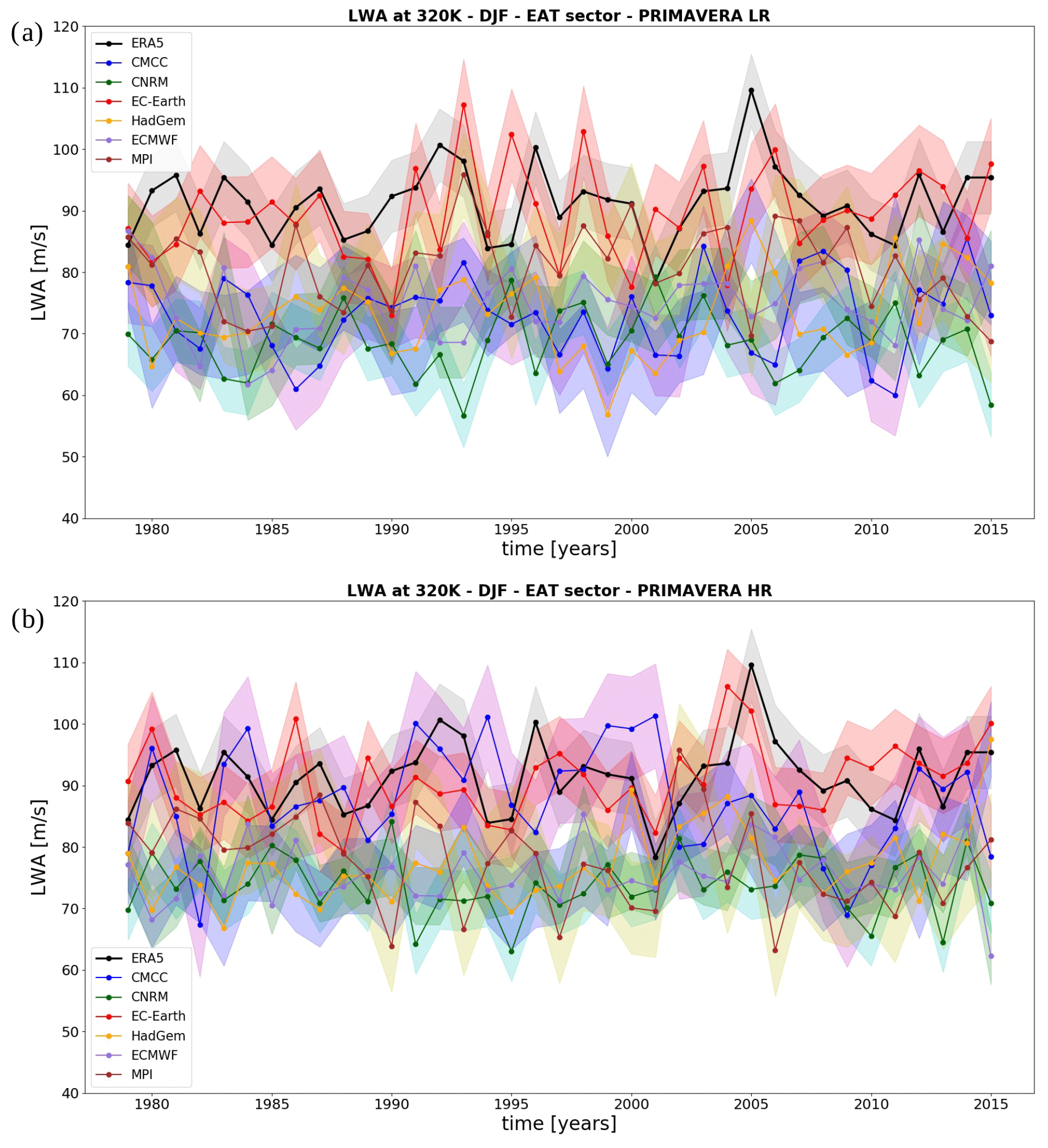
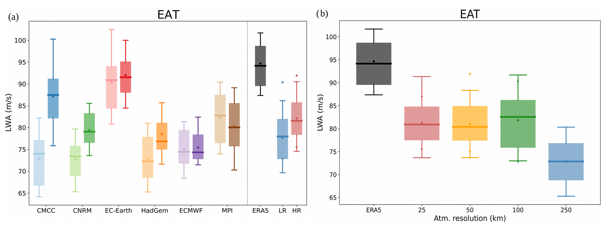
As we did for the whole NH, we now examine the temporal behaviour of transient LWA, restricting our attention on the EAT sector, where WRs are computed. Figure 12 shows the time series of LWA averaged over the EAT sector for LR (Fig. 12a) and HR runs (Fig. 12b). In the EAT sector the magnitude of averaged LWA is stronger in the HR runs, but the gap between LR and HR appears less pronounced compared to the one observed in the NH, as can be seen in Fig. 13a. The MPI model again is the only model in which the HR run exhibits less LWA than the LR. ECMWF and EC-Earth do not show an increase in LWA between LR and HR, whereas HadGEM, CNRM and CMCC show an appreciable increase in the magnitude of the averaged LWA. Note how in the CMCC and CNRS models (which showed the largest increase in the LWA magnitude with resolution in both the NH and EAT sectors), the resolution of the HR run is considerably finer than the LR (refer to Table 1). In the EAT sector the convergence of the averaged transient LWA magnitude towards the observations with horizontal resolution appears less evident than in the NH (Fig. 13b); a first increase is observed between 250 and 100 km, and then the LWA remains almost constant as the resolution is further increased. Also, in this case no evident Rossby wave activity trend can be found in the time series in both the observations and LR and HR simulations (p values for Mann–Kendall test are 0.20 for ERA5, between 0.13 and 0.96 for PRIMAVERA LR, and between 0.27 and 0.76 for PRIMAVERA HR).
In this work we have analysed the performance of state-of-the-art climate models in representing the recurrent large-scale circulation patterns associated with Rossby waves in the NH and EAT sectors during winter. In particular, the impact of an increased resolution on the representation of the large-scale atmospheric dynamics on the PRIMAVERA coupled climate simulations in the historical runs has been assessed. Reanalysis data (ERA5), covering the 1979–2015 period, have been used as reference. In all models apart from two (CMCC and MPI), the horizontal resolution is increased in both the atmosphere and the ocean, whereas in the CMCC and MPI models only the atmospheric resolution is increased. Our approach combined the diagnostic for Rossby waves based on the LWA in isentropic coordinates of Ghinassi et al. (2018), to quantify their amplitude and a weather regime analysis (following Fabiano et al., 2020) to subsequently compute WRs over the EAT sector.
Firstly, we computed LWA for the whole NH, to analyse the large-scale wintertime circulation in terms of Rossby wave activity in the reanalysis dataset. The LWA diagnostic is particularly suited to capture the large-scale dynamics that characterize the Pacific and North Atlantic storm tracks and identifies them in terms of Rossby wave activity associated with planetary waves and transient RWPs. The same analysis performed on the PRIMAVERA multimodel mean of the LR and HR runs reveals an improvement in the ability of the models in representing the total LWA spatial distribution in the HR, but the same is not true for transient LWA. This has been attributed to a better representation of stationary LWA in the HR set; on the other hand, when examining transient LWA, we concluded that a further analysis was needed to enlighten whether the minimal improvement of the HR was a common characteristic of all models or a result of cancellation arising from the multimodel mean.
The temporal variability of Rossby wave activity has been analysed, also producing time series of spatially averaged transient LWA for the NH. It is evident how PRIMAVERA models tend to underestimate the magnitude of the spatially averaged LWA compared to reanalysis. In this case an increased horizontal resolution is clearly beneficial, since the magnitude of LWA in the HR simulations is closer to the reanalysis in all models apart from one (the MPI model). We also examined the dependence of LWA with resolution, and we found clear evidence of the LWA magnitude converging to the observed one upon increasing the horizontal atmospheric resolution. No significant trends in the evolution of LWA are found in either the observations or PRIMAVERA historical simulations (LR and HR). The evidence for no wave activity trends in the observation is in agreement with the analysis of Blackport and Screen (2020), who diagnosed waviness using a LWA variant based on geopotential height and with the analysis of Souders et al. (2014), who also investigated trends in RWP frequency, activity and amplitude using a diagnostic based on the envelope of meridional wind. It is worth noting that our results are not consistent with that of Francis and Vavrus (2012, 2015), where a recent increase in the midlatitudes waviness due to Arctic amplification was claimed. However these authors quantified the Rossby wave amplitude using a predefined set of geopotential height isopleths, which may vary in time even due to conservative dynamics (since geopotential is not conserved). This makes it hard to tell whether the amplitude increase they have observed was related to natural variability of the geopotential height field or rather caused by diabatic processes in the lower troposphere. On the other hand, the conservation relation of isentropic LWA (i.e. based on Ertel PV) provides a straightforward link between the rate of change of LWA due to the effect of forcings such as diabatic and other nonconservative processes. The fact that no significant LWA increase or decrease is observed during the examined period thereby implies a net zero effect of the diabatic sources and sinks of LWA, which may have an impact on the Rossby wave dynamics in the extratropics. This suggests that there is “no winner” yet in the tug-of-war between a reduced temperature gradient in the lower troposphere (related to Arctic amplification) and an increased one in the upper levels (related to the warming of the upper troposphere in the tropics and the cooling of the lower stratosphere in polar regions), as discussed in Barnes and Screen (2015). All fluctuations observed in the reanalysis and PRIMAVERA (LR and HR) therefore appear to be associated with the intraseasonal variability of LWA.
In Sect. 4, we restricted our attention over the EAT sector. Using the WR tool, we partitioned the LWA associated with the four WRs over the EAT sector in the observations and in the LR and HR PRIMAVERA simulations. We examined the pattern of transient LWA associated with each WR and compared it to the observations. Apart from one model (CMCC model for the AR regime) the pattern correlation shows that the large-scale pattern associated with each WR is in good agreement (values larger than 0.6) with the observations. The WRs with the highest values of pattern correlations amongst the set of models are SB and NAO−. An improvement of the LWA pattern correlation in the HR simulations is not systematically observed in all models: some models show no improvement in the pattern correlation between the LR and HR simulations, and in some of the cases (CMCC and MPI) the HR runs have a lower pattern correlation for some of the regimes. If the LWA pattern correlation provides a concise metric to assess the model performance, it cannot reveal whether the error committed by a model in reproducing the spatial distribution of LWA arises from the misrepresentation of the wave amplitude or in a shift in its phase. For this reason we examined LWA and Montgomery stream function anomaly maps, and we observed how LWA associated with each regime in the reanalysis appears very localized in space. LWA indeed maximizes in the vicinity of the positive and negative M anomalies characteristic of each regime pattern and decays to smaller values farther away. In the PRIMAVERA models instead, the magnitude of such LWA maxima generally appears weaker compared with the observations. Furthermore some models, in spite of having high values of pattern correlation over the considered sector, fail to represent the LWA pattern in other regions of the NH. In particular, when examining the NAO+ pattern, we found that the majority of the models underestimate the magnitude of LWA associated with anticyclonic wavebreaking located over Europe and the Mediterranean. This area of anticyclonic LWA in fact appears too weak over these regions, suggesting that the models do not correctly simulate Rossby wavebreaking and the decay of RWPs over Europe and the Mediterranean, which instead continue their eastward propagation. When examining the SB, we found that two of the models which showed a substantial improvement in the LWA magnitude and pattern are ECMWF and CNRS. The HR runs of these models have a substantial increase in the horizontal resolution of both the atmosphere and the ocean. Another commonly observed feature amongst the models is the difficulty in representing the area of high LWA on the western flank of the anticyclones, resulting in the LWA core being too shifted to the east. This suggests that the models fail to reproduce the upstream transient LWA “accumulation” into the large amplitude ridges, which characterizes the onset and maintenance of blocking (Altenhoff et al., 2008; Nakamura and Huang, 2018) at the right location. A similar behaviour was observed by Quinting and Vitart (2019) in the analysis of RWPs and blocking in the S2S database and was attributed to a negative RWP decay frequency and blocking frequency biases over the EAT region. A possible mechanism to explain this misrepresentation of LWA in the models is related to the tendency of the models to have a weaker PV gradient at the tropopause (which is directly related to the magnitude of LWA) due to numerical diffusion (Gray et al., 2014; Harvey et al., 2018). Finally, there were some examples of models which almost completely fail to reproduce the observed Rossby wave activity pattern. This happens for example for the SB regime in the CMCC HR and NAO− in MPI HR. A worse performance of the CMCC HR compared to LR in the representation of European–Atlantic blocking was also observed by Schiemann et al. (2020). Over the Pacific and western portion of North America a secondary LWA maximum associated with Rossby wave activity located downstream over the EAT sector is observed in the reanalysis for all regimes. This feature has not been found in any of the PRIMAVERA simulations, suggesting that the models miss the teleconnection associated with a Rossby wave train extending from the Pacific Ocean to the North Atlantic. These differences in how the models simulate the large-scale circulation in the upper troposphere have implications since they are likely to be associated with errors in the circulation near the surface.
The analysis of the temporal evolution of the spatially averaged Rossby wave activity over the EAT sector reveals that as for the NH the HR simulations have a LWA magnitude which is closer to reanalysis, apart from the MPI model. In the EAT sector however the gap in the LWA magnitude between HR and LR is smaller compared to the NH, and the dependence of the LWA magnitude on the horizontal atmospheric resolution is not as evident as it is for the whole NH. Finally, also in this case no significant wave activity trends are visible in the EAT sector.
Concluding, the models in which the horizontal resolution was increased simultaneously in the atmosphere and in the ocean generally show an improvement in the representation of Rossby wave activity. Notably, in the CMCC and MPI models, in which an increased horizontal resolution degraded the model performance in simulating the spatial and temporal variability of Rossby wave activity, the resolution was increased only in the atmosphere but was left unchanged in the ocean.
The same analysis but in terms of anomalous transient LWA, which can be found in the Supplement, also confirmed the results discussed above.
Obviously our analysis focused only on the large-scale circulation in the upper troposphere and does not provide information on possible biases in the dynamics at lower or higher altitudes, or happening on a spatio-temporal scale smaller than the synoptic scale. In future work we will examine how the observed model biases in the upper-tropospheric Rossby wave activity are connected with surface weather and extend our diagnostic framework to future climate simulations.
As discussed in Sect. 2.2, LWA is partly Lagrangian in latitude and altitude. This arises from the fact that isentropic surfaces evolve with time according to the variations in temperature. Since in this analysis we are comparing observations and models with different mean states, we want to first verify that the considered isentrope intersects the tropopause in the midlatitudes, which is a desirable property to identify RWPs with LWA (Ghinassi et al., 2018), and secondly that the height of such an isentropic surface does not differ considerably between ERA5 and the models. Figure A1 shows the time-zonal mean of the 320 K isentrope in the observations and PRIMAVERA LR simulations. It can be seen how the tropopause (associated with the marked change in the isentrope slope associated with a higher static stability in the stratosphere) is intercepted at around 250 hPa in the midlatitudes (around 45∘ N) of the NH in ERA5 and the majority of PRIMAVERA models. A notable exception is the CNRM model in which the 320 K isentropic surface is located at a higher altitude in the troposphere, presumably due to a bias in the mean temperature. Note the bias in the height of the tropopause in the Southern Hemisphere, presumably related with a too-cold lower stratosphere during summer in the PRIMAVERA simulations (the same feature is observed in NH during JJA, not shown here). However, since our analysis focuses on the NH during winter this bias does not affect our results and will not be investigate further.
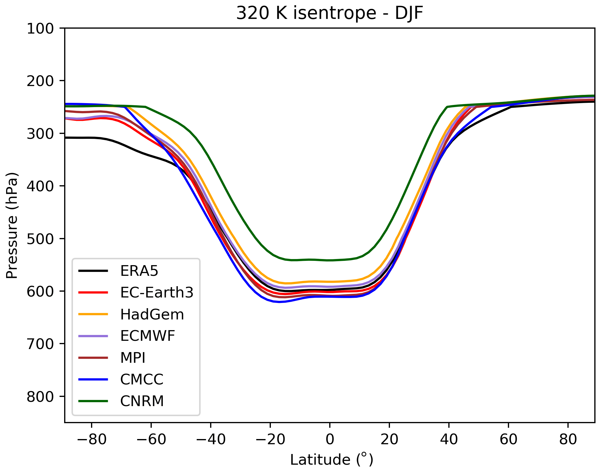
Figure A1Pressure height (in hPa) of the 320 K isentropic surface (time-zonal mean for DJF). The black line is ERA5, and other colours are PRIMAVERA LR simulations.
The WRtool package is freely available at https://doi.org/10.5281/zenodo.4590985 (Fabiano and Mavilia, 2021). The code to compute LWA from meteorological data is available from the authors upon request.
The supplement related to this article is available online at: https://doi.org/10.5194/wcd-3-209-2022-supplement.
PG conducted most of the data analyses and visualizations and drafted the paper. FF performed part of the data analysis and visualizations. PG, FF and SC all commented on, organized and wrote parts of the paper.
The contact author has declared that neither they nor their co-authors have any competing interests.
Publisher's note: Copernicus Publications remains neutral with regard to jurisdictional claims in published maps and institutional affiliations.
The authors thank the two anonymous reviewers for their comments and suggestions that significantly improved the paper. The authors acknowledge support by the PRIMAVERA project. The climate model simulations used in this study were performed under the PRIMAVERA project and can be accessed at the archive of the Centre for Environmental Data Analysis (CEDA). The authors also acknowledge the extensive use of the supercomputer at CINECA under the framework of the Climate-SPHINX reloaded PRACE project and the CEDA-JASMIN platform for enabling data storage and model analysis. The authors also acknowledge the JPI Ocean-Climate Project ROADMAP.
This research has been supported by the Horizon 2020 programme (grant no. PRIMAVERA (641727)).
This paper was edited by Gwendal Rivière and reviewed by two anonymous referees.
Altenhoff, A., Martius, O., Croci-Maspoli, M., Schwierz, C., and Davies, H.: Linkage of atmospheric blocks and synoptic-scale Rossby waves: A climatological analysis, Tellus A, 60, 1053–1063, https://doi.org/10.1111/j.1600-0870.2008.00354.x, 2008. a
Andrews, D. and Mcintyre, M. E.: Planetary waves in horizontal and vertical shear: The generalized Eliassen–Palm relation and the mean zonal acceleration, J. Atmos. Sci., 33, 2031–2048, https://doi.org/10.1175/1520-0469(1976)033<2031:PWIHAV>2.0.CO;2, 1976. a
Andrews, D. G., Holton, J. R., and Leovy, C. B.: Middle Atmosphere Dynamics, Academic Press, 489 pp., Volume 40, International Geophysics Series, 1987. a
Barnes, E. A.: Revisiting the evidence linking Arctic amplification to extreme weather in midlatitudes, Geophys. Res. Lett., 40, 4734–4739, https://doi.org/10.1002/grl.50880, 2013. a
Barnes, E. A. and Screen, J. A.: The impact of Arctic warming on the midlatitude jet-stream: Can it? Has it? Will it?, WIREs Clim. Change, 6, 277–286, 2015. a, b
Baumgart, M., Ghinassi, P., Wirth, V., Selz, T., Craig, G. C., and Riemer, M.: Quantitative view on the processes governing the upscale error growth up to the planetary scale using a stochastic convection scheme, Mon. Weather Rev., 147, 1713–1731, https://doi.org/10.1175/MWR-D-18-0292.1, 2019. a
Blackmon, M. L.: A Climatological Spectral Study of the 500 mb Geopotential Height of the Northern Hemisphere, J. Atmos. Sci., 33, 1607–1623, https://doi.org/10.1175/1520-0469(1976)033<1607:ACSSOT>2.0.CO;2, 1976. a
Blackmon, M. L., Lee, Y., and Wallace, J. M.: Horizontal structure of 500 mb height fluctuations with long, intermediate and short time scales, J. Atmos. Sci., 41, 961–980, 1984. a
Blackport, R. and Screen, J. A.: Insignificant effect of Arctic amplification on the amplitude of midlatitude atmospheric waves, Science Advances, 6, eaay2880, https://doi.org/10.1126/sciadv.aay2880, 2020. a, b
Branstator, G.: Circumglobal Teleconnections, the Jet Stream Waveguide, and the North Atlantic Oscillation, J. Climate, 5, 1893–1910, https://doi.org/10.1175/1520-0442(2002)015<1893:CTTJSW>2.0.CO;2, 2002. a
Cassou, C.: Intraseasonal interaction between the Madden–Julian oscillation and the North Atlantic Oscillation, Nature, 455, 523–527, https://doi.org/10.1038/nature07286, 2008. a, b
Cassou, C., Minvielle, M., Terray, L., and Perigaud, C.: A statistical–dynamical scheme for reconstructing ocean forcing in the Atlantic. Part I: weather regimes as predictors for ocean surface variables, Clim. Dynam., 36, 19–39, https://doi.org/10.1007/s00382-010-0781-7, 2010. a
Cattiaux, J., Douville, H., and Peings, Y.: European temperatures in CMIP5: origins of present-day biases and future uncertainties, Clim. Dynam., 41, 2889–2907, 2013. a
Chang, E. K. M. and Orlanski, I.: On the Dynamics of a Storm Track, J. Atmos. Sci., 50, 999–1015, https://doi.org/10.1175/1520-0469(1993)050<0999:OTDOAS>2.0.CO;2, 1993. a
Charney, J. G. and Drazin, P. G.: Propagation of planetary-scale disturbances from the lower into the upper atmosphere, J. Geophys. Res., 66, 83–109, 1961. a
Chen, G., Lu, J., Burrows, D. A., and Leung, L. R.: Local finite-amplitude wave activity as an objective diagnostic of midlatitude extreme weather, Geophys. Res. Lett., 42, 10952–10960, https://doi.org/10.1002/2015GL066959, 2015. a, b
Cherchi, A., Fogli, P. G., Lovato, T., Peano, D., Iovino, D., Gualdi, S., Masina, S., Scoccimarro, E., Materia, S., Bellucci, A., and Navarra, A.: Global Mean Climate and Main Patterns of Variability in the CMCC-CM2 Coupled Model, J. Adv. Model. Earth Sy., 11, 185–209, https://doi.org/10.1029/2018MS001369, 2019. a
Corti, S., Molteni, F., and Palmer, T.: Signature of recent climate change in frequencies of natural atmospheric circulation regimes, Nature, 398, 799–802, https://doi.org/10.1038/19745, 1999. a
Dawson, A., Palmer, T., and Corti, S.: Simulating regime structures in weather and climate prediction models, Geophys. Res. Lett., 39, L21805, https://doi.org/10.1029/2012GL053284, 2012. a
Edmon Jr, H., Hoskins, B., and McIntyre, M.: Eliassen–Palm cross sections for the troposphere, J. Atmos. Sci., 37, 2600–2616, 1980. a
Ertel, H.: Ein neuer hydrodynamischer Wirbelsatz, Meteorol. Z., 59, 277–281, 1942. a
Fabiano, F. and Mavilia, I: fedef17/WRtool: WRtool 2.1 (v2.1), Zenodo [code], https://doi.org/10.5281/zenodo.4590985, 2021. a
Fabiano, F., Christensen, H., Strommen, K., Athanasiadis, P., Baker, A., Schiemann, R., and Corti, S.: Euro–Atlantic weather Regimes in the PRIMAVERA coupled climate simulations: impact of resolution and mean state biases on model performance, Clim. Dynam., 54, 5031–5048, https://doi.org/10.1007/s00382-020-05271-w, 2020. a, b, c, d, e, f, g, h, i, j
Fabiano, F., Meccia, V. L., Davini, P., Ghinassi, P., and Corti, S.: A regime view of future atmospheric circulation changes in northern mid-latitudes, Weather Clim. Dynam., 2, 163–180, https://doi.org/10.5194/wcd-2-163-2021, 2021. a, b
Francis, J. A. and Vavrus, S. J.: Evidence linking Arctic amplification to extreme weather in mid-latitudes, Geophys. Res. Lett., 39, L06801, https://doi.org/10.1029/2012GL051000, 2012. a, b, c
Francis, J. A. and Vavrus, S. J.: Evidence for a wavier jet stream in response to rapid Arctic warming, Environ. Res. Lett., 10, 014005, https://doi.org/10.1088/1748-9326/10/1/014005, 2015. a, b
Ghinassi, P., Fragkoulidis, G., and Wirth, V.: Local Finite-Amplitude Wave Activity as a Diagnostic for Rossby Wave Packets, Mon. Weather Rev., 146, 4099–4114, https://doi.org/10.1175/MWR-D-18-0068.1, 2018. a, b, c, d, e, f, g, h, i
Ghinassi, P., Baumgart, M., Teubler, F., Riemer, M., and Wirth, V.: A Budget Equation for the Amplitude of Rossby Wave Packets Based on Finite-Amplitude Local Wave Activity, J. Atmos. Sci., 77, 277–296, 2020. a, b
Gray, S. L., Dunning, C. M., Methven, J., Masato, G., and Chagnon, J. M.: Systematic model forecast error in Rossby wave structure, Geophys. Res. Lett., 41, 2979–2987, https://doi.org/10.1002/2014GL059282, 2014. a
Gutjahr, O., Putrasahan, D., Lohmann, K., Jungclaus, J. H., von Storch, J.-S., Brüggemann, N., Haak, H., and Stössel, A.: Max Planck Institute Earth System Model (MPI-ESM1.2) for the High-Resolution Model Intercomparison Project (HighResMIP), Geosci. Model Dev., 12, 3241–3281, https://doi.org/10.5194/gmd-12-3241-2019, 2019. a
Haarsma, R., Acosta, M., Bakhshi, R., Bretonnière, P.-A., Caron, L.-P., Castrillo, M., Corti, S., Davini, P., Exarchou, E., Fabiano, F., Fladrich, U., Fuentes Franco, R., García-Serrano, J., von Hardenberg, J., Koenigk, T., Levine, X., Meccia, V. L., van Noije, T., van den Oord, G., Palmeiro, F. M., Rodrigo, M., Ruprich-Robert, Y., Le Sager, P., Tourigny, E., Wang, S., van Weele, M., and Wyser, K.: HighResMIP versions of EC-Earth: EC-Earth3P and EC-Earth3P-HR – description, model computational performance and basic validation, Geosci. Model Dev., 13, 3507–3527, https://doi.org/10.5194/gmd-13-3507-2020, 2020. a, b
Harvey, B., Methven, J., and Ambaum, M. H. P.: An Adiabatic Mechanism for the Reduction of Jet Meander Amplitude by Potential Vorticity Filamentation, J. Atmos. Sci., 75, 4091–4106, https://doi.org/10.1175/JAS-D-18-0136.1, 2018. a
Hersbach, H., Bell, B., Berrisford, P., Hirahara, S., Horányi, A., Muñoz-Sabater, J., Nicolas, J., Peubey, C., Radu, R., Schepers, D., Simmons, A., Soci, C., Abdalla, S., Abellan, X., Balsamo, G., Bechtold, P., Biavati, G., Bidlot, J., Bonavita, M., De Chiara, G., Dahlgren, P., Dee, D., Diamantakis, M., Dragani, R., Flemming, J., Forbes, R., Fuentes, M., Geer, A., Haimberger, L., Healy, S., Hogan, R. J., Hólm, E., Janisková, M., Keeley, S., Laloyaux, P., Lopez, P., Lupu, C., Radnoti, G., de Rosnay, P., Rozum, I., Vamborg, F., Villaume, S., and Thépaut, J.-N.: The ERA5 global reanalysis, Q. J. Roy. Meteor. Soc., 146, 1999–2049, https://doi.org/10.1002/qj.3803, 2020. a
Hoskins, B. J. and Karoly, D. J.: The Steady Linear Response of a Spherical Atmosphere to Thermal and Orographic Forcing, J. Atmos. Sci., 38, 1179–1196, https://doi.org/10.1175/1520-0469(1981)038<1179:TSLROA>2.0.CO;2, 1981. a
Hoskins, B. J., McIntyre, M. E., and Robertson, A. W.: On the use and significance of isentropic potential vorticity maps, Q. J. Roy. Meteor. Soc., 111, 877–946, https://doi.org/10.1002/qj.49711147002, 1985. a, b
Huang, C. S. Y. and Nakamura, N.: Local Finite-Amplitude Wave Activity as a Diagnostic of Anomalous Weather Events, J. Atmos. Sci., 73, 211–229, https://doi.org/10.1175/JAS-D-15-0194.1, 2016. a, b, c, d, e
Huang, C. S. Y. and Nakamura, N.: Local wave activity budgets of the wintertime Northern Hemisphere: Implications for the Pacific and Atlantic storm tracks, Geophys. Res. Lett., 44, 5673–5682, https://doi.org/10.1002/2017GL073760, 2017. a
Ivy, D. J., Solomon, S., and Rieder, H. E.: Radiative and Dynamical Influences on Polar Stratospheric Temperature Trends, J. Climate, 29, 4927–4938, https://doi.org/10.1175/JCLI-D-15-0503.1, 2016. a
Lee, S. and Held, I. M.: Baroclinic wave packets in models and observations, J. Atmos. Sci., 50, 1413–1428, https://doi.org/10.1175/1520-0469(1993)050<1413:BWPIMA>2.0.CO;2, 1993. a
Li, Y., Yang, S., Deng, Y., Hu, X., Cai, M., and Zhou, W.: Detection and attribution of upper-tropospheric warming over the tropical western Pacific, Clim. Dynam., 53, 3057–3068, 2019. a
Martius, O., Schwierz, C., and Davies, H.: Breaking waves at the tropopause in the wintertime Northern Hemisphere: Climatological analyses of the orientation and the theoretical LC1/2 classification, J. Atmos. Sci., 64, 2576–2592, 2007. a
Matsueda, M. and Palmer, T.: Estimates of flow-dependent predictability of wintertime Euro–Atlantic weather regimes in medium-range forecasts, Q. J. Roy. Meteor. Soc., 144, 1012–1027, 2018. a
Michelangeli, P.-A., Vautard, R., and Legras, B.: Weather regimes: Recurrence and quasi stationarity, J. Atmos. Sci., 52, 1237–1256, 1995. a, b
Nakamura, N. and Huang, C. S. Y.: Atmospheric blocking as a traffic jam in the jet stream, Science, 361, 42–47, https://doi.org/10.1126/science.aat0721, 2018. a
Nakamura, N. and Solomon, A.: Finite-amplitude wave activity and mean flow adjustments in the atmospheric general circulation. Part I: Quasigeostrophic theory and analysis, J. Atmos. Sci., 67, 3967–3983, https://doi.org/10.1175/2010JAS3503.1, 2010. a, b
Nakamura, N. and Zhu, D.: Finite-amplitude wave activity and diffusive flux of potential vorticity in eddy–mean flow interaction, J. Atmos. Sci., 67, 2701–2716, https://doi.org/10.1175/2010JAS3432.1, 2010. a
Novak, L., Ambaum, M. H., and Tailleux, R.: The life cycle of the North Atlantic storm track, J. Atmos. Sci., 72, 821–833, 2015. a
Pedlosky, J.: Finite-Amplitude Baroclinic Wave Packets, J. Atmos. Sci., 29, 680–686, https://doi.org/10.1175/1520-0469(1972)029<0680:FABWP>2.0.CO;2, 1972. a
Quinting, J. F. and Vitart, F.: Representation of Synoptic-Scale Rossby Wave Packets and Blocking in the S2S Prediction Project Database, Geophys. Res. Lett., 46, 1070–1078, https://doi.org/10.1029/2018GL081381, 2019. a
Randel, W. J. and Wu, F.: Cooling of the Arctic and Antarctic polar stratospheres due to ozone depletion, J. Climate, 12, 1467–1479, https://doi.org/10.1175/1520-0442(1999)012<1467:COTAAA>2.0.CO;2, 1999. a
Roberts, C. D., Senan, R., Molteni, F., Boussetta, S., Mayer, M., and Keeley, S. P. E.: Climate model configurations of the ECMWF Integrated Forecasting System (ECMWF-IFS cycle 43r1) for HighResMIP, Geosci. Model Dev., 11, 3681–3712, https://doi.org/10.5194/gmd-11-3681-2018, 2018. a
Robertson, A. W. and Ghil, M.: Large-Scale Weather Regimes and Local Climate over the Western United States, J. Climate, 12, 1796–1813, https://doi.org/10.1175/1520-0442(1999)012<1796:LSWRAL>2.0.CO;2, 1999. a
Scaife, A. A., Camp, J., Comer, R., Davis, P., Dunstone, N., Gordon, M., MacLachlan, C., Martin, N., Nie, Y., Ren, H.-L., Roberts, M., Robinson, W., Smith, D., and Vidale, P. L.: Does increased atmospheric resolution improve seasonal climate predictions?, Atmos. Sci. Lett., 20, e922, https://doi.org/10.1002/asl.922, 2019. a
Schiemann, R., Athanasiadis, P., Barriopedro, D., Doblas-Reyes, F., Lohmann, K., Roberts, M. J., Sein, D. V., Roberts, C. D., Terray, L., and Vidale, P. L.: Northern Hemisphere blocking simulation in current climate models: evaluating progress from the Climate Model Intercomparison Project Phase 5 to 6 and sensitivity to resolution, Weather Clim. Dynam., 1, 277–292, https://doi.org/10.5194/wcd-1-277-2020, 2020. a
Screen, J. A. and Simmonds, I.: The central role of diminishing sea ice in recent Arctic temperature amplification, Nature, 464, 1334–1337, 2010. a
Screen, J. A. and Simmonds, I.: Exploring links between Arctic amplification and mid-latitude weather, Geophys. Res. Lett., 40, 959–964, https://doi.org/10.1002/grl.50174, 2013. a
Serreze, M. C., Barrett, A. P., Stroeve, J. C., Kindig, D. N., and Holland, M. M.: The emergence of surface-based Arctic amplification, The Cryosphere, 3, 11–19, https://doi.org/10.5194/tc-3-11-2009, 2009. a
Simmons, A. J. and Hoskins, B. J.: The downstream and upstream development of unstable baroclinic waves, J. Atmos. Sci., 36, 1239–1254, https://doi.org/10.1175/1520-0469(1979)036<1239:TDAUDO>2.0.CO;2, 1979. a
Souders, M. B., Colle, B. A., and Chang, E. K. M.: A Description and Evaluation of an Automated Approach for Feature-Based Tracking of Rossby Wave Packets, Mon. Weather Rev., 142, 3505–3527, https://doi.org/10.1175/MWR-D-13-00317.1, 2014. a
Straus, D. M., Corti, S., and Molteni, F.: Circulation regimes: Chaotic variability versus SST-forced predictability, J. Climate, 20, 2251–2272, 2007. a
Strommen, K., Mavilia, I., Corti, S., Matsueda, M., Davini, P., von Hadenberg, J., Vidale, P., and Mizuta, R.: The Sensitivity of Euro–Atlantic Regimes to Model Horizontal Resolution, arXiv [preprint], arXiv:1905.07046, 2019. a
Strong, C. and Magnusdottir, G.: Tropospheric Rossby wave breaking and the NAO/NAM, J. Atmos. Sci., 65, 2861–2876, 2008. a
Voldoire, A., Saint-Martin, D., Sénési, S., Decharme, B., Alias, A., Chevallier, M., Colin, J., Guérémy, J.-F., Michou, M., Moine, M.-P., Nabat, P., Roehrig, R., Salas y Mélia, D., Séférian, R., Valcke, S., Beau, I., Belamari, S., Berthet, S., Cassou, C., Cattiaux, J., Deshayes, J., Douville, H., Ethé, C., Franchistéguy, L., Geoffroy, O., Lévy, C., Madec, G., Meurdesoif, Y., Msadek, R., Ribes, A., Sanchez-Gomez, E., Terray, L., and Waldman, R.: Evaluation of CMIP6 DECK Experiments With CNRM-CM6-1, J. Adv. Model. Earth Sy., 11, 2177–2213, https://doi.org/10.1029/2019MS001683, 2019. a
Wallace, J. M. and Gutzler, D. S.: Teleconnections in the Geopotential Height Field during the Northern Hemisphere Winter, Mon. Weather Rev., 109, 784–812, https://doi.org/10.1175/1520-0493(1981)109<0784:TITGHF>2.0.CO;2, 1981. a
Wernli, H. and Sprenger, M.: Identification and ERA-15 Climatology of Potential Vorticity Streamers and Cutoffs near the Extratropical Tropopause, J. Atmos. Sci., 64, 1569–1586, https://doi.org/10.1175/JAS3912.1, 2007. a
Williams, K. D., Copsey, D., Blockley, E. W., Bodas-Salcedo, A., Calvert, D., Comer, R., Davis, P., Graham, T., Hewitt, H. T., Hill, R., Hyder, P., Ineson, S., Johns, T. C., Keen, A. B., Lee, R. W., Megann, A., Milton, S. F., Rae, J. G. L., Roberts, M. J., Scaife, A. A., Schiemann, R., Storkey, D., Thorpe, L., Watterson, I. G., Walters, D. N., West, A., Wood, R. A., Woollings, T., and Xavier, P. K.: The Met Office Global Coupled Model 3.0 and 3.1 (GC3.0 and GC3.1) Configurations, J. Adv. Model. Earth Sy., 10, 357–380, https://doi.org/10.1002/2017MS001115, 2018. a
Wirth, V., Riemer, M., Chang, E. K. M., and Martius, O.: Rossby Wave Packets on the Midlatitude Waveguide–A Review, Mon. Weather Rev., 146, 1965–2001, https://doi.org/10.1175/MWR-D-16-0483.1, 2018. a, b
Yiou, P. and Nogaj, M.: Extreme climatic events and weather regimes over the North Atlantic: When and where?, Geophys. Res. Lett., 31, L07202, https://doi.org/10.1029/2003GL019119, 2004. a, b
- Abstract
- Introduction
- Theory and methodology
- Wintertime Rossby wave activity in the Northern Hemisphere
- Wintertime Rossby wave activity over the European–Atlantic sector
- Discussion and conclusions
- Appendix A: Potential temperature profiles in the PRIMAVERA simulations
- Code availability
- Author contributions
- Competing interests
- Disclaimer
- Acknowledgements
- Financial support
- Review statement
- References
- Supplement